The band-centre anomaly in the 1D Anderson model with correlated disorder

Abstract

We study the band-centre anomaly in the one-dimensional Anderson model with weak correlated disorder. Our analysis is based on the Hamiltonian map approach; the correspondence between the discrete model and its continuous counterpart is discussed in detail. We obtain analytical expressions of the localisation length and of the invariant measure of the phase variable, valid for energies in a neighbourhood of the band centre. By applying these general results to specific forms of correlated disorder, we show how correlations can enhance or suppress the anomaly at the band centre.

Pacs: 71.23.An, 72.15.Rn, 05.40.-a

1 Introduction

The one-dimensional (1D) Anderson model, first introduced in 1958 [1], remains the focus of active research. The analysis of this model showed that all eigenstates are exponentially localised for infinitely large samples (see, e.g., the reviews [2, 3]). For the case of weak and uncorrelated disorder, Thouless derived the expression for the localisation length that now bears his name [4]. Numerical calculations, however, revealed that Thouless’ expression fails at the band centre, where the actual localisation length was numerically found to be different from the expected value [5]. As was understood by Kappus and Wegner [6], this discrepancy is due to the failure of the Born approximation; with the use of a quite sophisticated method, Kappus and Wegner derived an approximate expression which explained the numerical data reported in Ref. [5]. Later on, using a different approach, Derrida and Gardner showed [7] that this anomaly is a resonance effect that emerges at the band centre, $E=0$. They also found another anomaly for $E=\pm 1$ and suggested that similar anomalies should appear for other resonant energies defined by $E=2\cos(\pi p/q)$, where $p$ and $q$ are integer number. The results of Ref. [7] were subsequently extended to a whole neighbourhood of the band centre [8, 9] (see also the discussion in Ref. [10]).

The interest in the anomalies of the Anderson model was raised significantly after these anomalies were linked to the so-called single-parameter scaling theory (SPS). The SPS theory was proposed in Ref. [11, 12] and was based on the random phase approximation (RPA) for the phases of the scattered waves. In the 1D case, the SPS theory can be reduced to the statement that all moments of the transmission coefficient through a random barrier can be expressed in terms of the first two moments. As a result, the whole distribution of the transmission coefficient is expected to depend on the ratio between the localisation length and the size of the random chain. However, it was numerically shown long ago [13] that the RPA fails at the band centre of the Anderson model. Thus, the band centre anomaly (as well as the other resonances) can serve as a touchstone for the study of the SPS hypothesis. As was recently shown in Ref. [14], the SPS hypothesis is violated also for the resonance at $E=\pm 1$ (see also the discussion in Refs. [15]). Since the phase distribution is not flat whenever the energy lies in a whole neighbourhood of the resonant values, one can expect that the SPS hypothesis should not be rigorously valid in the whole energy band of the 1D Anderson model with weak disorder. This “anti-SPS” hypothesis is still not proved; the study of the anomalies of the Anderson model for $E=0$ and $E=\pm 1$ can provide a way to test the validity of this conjecture.

The works on the band-centre anomaly mentioned so far considered the Anderson model with uncorrelated disorder. In the literature, almost no attention has been given to the case of correlated disorder, the main exception being Ref. [16] which, however, was focused on specific cases of very short-ranged correlations. Only very recently the effects of correlated disorder on the localisation of the band-centre states have begun to be investigated, in the wake of the discovery that the band-centre anomaly can be strongly reduced if the site energies exhibit exponentially decaying, positive correlations [17].

In this work we derive analytical results that show how the band-centre anomaly is modified when disorder possesses arbitrary correlations. The general expressions that we obtained allow us to treat the correlations considered in [17] as a particular case and to show how, in general, different kinds of disorder correlations can either enhance or suppress the anomaly at the centre of the energy band. To derive an analytical expression for the localisation length in a neighbourhood of the band centre, we relied on the Hamiltonian map formalism [18, 10] and we replaced a map for the angle variable with its continuum limit. In order to do so, we had to establish a rigorous correspondence between random maps with intercorrelated coloured noises and stochastic differential equations with the same features. This led us to derive a discrete integration scheme for stochastic differential equations with self- and cross-correlated noises. This scheme is another important result of the present paper.

To analyse the band-centre anomaly we considered the behaviour of the localisation length and that of the probability distribution for the angle variable (which is equivalent to the scattering phase). Our analytical results show that disorder correlations shape the localisation length in a twofold way: on the one hand, the modulation of the phase distribution causes a deviation of the actual Lyapunov exponent from the value predicted by the expression first derived by Izrailev and Krokhin [19], which generalises Thouless’ formula to the case of correlated disorder. This discrepancy is a resonance effect and represents the “anomaly” in the presence of correlated disorder. On the other hand, disorder correlations modify the localisation length via the power-spectrum factor which is already present in the formula obtained by Izrailev and Krokhin in Ref. [19]. By manipulating this factor, one can produce very strong localisation or effective delocalisation of the band-centre states.

The modulation of the phase distribution close to the band centre is the hallmark of the anomaly that occurs there. Our analytical expressions show that positive, exponentially decaying correlations of the disorder flatten the invariant distribution, thereby reducing the anomaly, as observed in [17]. The opposite effect occurs when correlations decrease exponentially in magnitude but oscillate between positive and negative values. Such correlations strongly enhance the band-centre anomaly. To complete the picture, we consider a third type of correlations, which describe a lattice formed by two statistically independent and physically interpenetrating sublattices. We show that these correlations do not alter the modulation of the invariant distribution with respect to the case of uncorrelated disorder; however, they can increase or decrease the energy interval over which the anomaly is significant.

This paper is organised as follows. In Sec. 2 we define the model under study and we introduce the Hamiltonian map approach. In Sec. 3 we show how to replace the random map for the phase variable with a corresponding stochastic differential equation. We proceed to derive general analytical expressions for the phase distribution and the localisation length in Sec. 4. After recovering the known results for the limit case of uncorrelated disorder in Sec. 5, we consider the case of disorder with positive and exponentially decreasing correlations in Sec. 6. The case of correlations oscillating between positive and negative values and with exponentially decreasing magnitude is discussed in Sec. 7. A case of long-ranged correlations is analysed in Sec. 8. We finally draw our conclusions in Sec. 9.

2 The Hamiltonian map approach

2.1 Definition of the model

We consider the 1D Anderson model with weak and correlated disorder. The model is defined by the Schrödinger equation

$$\psi_{n+1}+\psi_{n-1}+\varepsilon_{n}\psi_{n}=E\psi_{n}$$ (1)

with random site energies $\varepsilon_{n}$. We use energy units such that $\hbar^{2}/2m=1$. We assume that

$$\begin{array}[]{ccc}\langle\varepsilon_{n}\rangle=0&\mbox{ and }&\langle\varepsilon_{n}^{2}\rangle=\sigma^{2}.\end{array}$$ (2)

We restrict our attention to the case of weak disorder, defined by the condition

$$\sigma^{2}\ll 1.$$ (3)

To complete the description of the statistical properties of the model (1), we introduce the normalised binary correlator

$$\frac{\langle\varepsilon_{n}\varepsilon_{n+l}\rangle}{\langle\varepsilon_{n}^{2}\rangle}=\chi(l).$$ (4)

Note that, in the weak-disorder limit, only the binary correlator (4) is required to define the statistical properties of the disorder (unless one wants to go beyond the second-order approximation). We assume that the system is spatially homogeneous in the mean; for this reason the binary correlator (4) depends only on the distance $l$ between the sites. We further assume disorder to be left-right symmetric on average so that $\chi(l)$ is an even function of $l$.

We further assume that the binary correlator $\chi(l)$ decreases quickly beyond a finite length scale $l_{c}$. This condition was not used in previous second-order analyses of the Anderson model with weak disorder [10]. It is needed here, however, to avoid mathematical inconsistencies in the application of the special technique which is required to deal with the compound problem of the band-centre anomaly in the presence of correlated disorder (see Sec. 4). We shall consider disorder to be weak enough that condition

$$\sigma^{2}l_{c}\ll 1$$ (5)

applies. In physical terms, this is equivalent to the assumption that the correlation length $l_{c}$ is much shorter than the localisation length. To deal with the case of long-ranged correlations, we shall derive results valid for any finite $l_{c}$ and then consider the limit $l_{c}\to\infty$, as discussed in Sec. 8.

2.2 The Hamiltonian map

The Hamiltonian map approach provides a useful way to study the structure of the electronic states of the Anderson model [20]. The approach is based on the analogy between the quantum model (1) and a classical parametric oscillator with Hamiltonian

$$H=\frac{p^{2}}{2m}+\frac{1}{2}m\omega^{2}x^{2}\left[1+\xi(t)\right]$$ (6)

where $\xi(t)$ is a succession of delta kicks of random strengths

$$\xi(t)=\sum_{n=-\infty}^{\infty}\xi_{n}\delta\left(t-nT\right).$$

The integration of the dynamical equations of the oscillator (6) over the period $T$ between two kicks leads to the Hamiltonian map

$$\begin{array}[]{ccl}x_{n+1}&=&\displaystyle\left[\cos\left(\omega T\right)-\omega\xi_{n}\sin\left(\omega T\right)\right]x_{n}+\frac{1}{m\omega}\sin\left(\omega T\right)p_{n}\\ p_{n+1}&=&\displaystyle-m\omega\left[\sin\left(\omega T\right)+\omega\xi_{n}\cos\left(\omega T\right)\right]x_{n}+\cos\left(\omega T\right)p_{n}.\end{array}$$ (7)

By eliminating the momenta from the map (7), one obtains the equation

$$x_{n+1}+x_{n-1}+\omega\xi_{n}\sin\left(\omega T\right)x_{n}=2\cos\left(\omega T\right)x_{n},$$

which coincides with the Schrödinger equation (1) for the Anderson model provided that

$$\begin{array}[]{ccc}E=2\cos\left(\omega T\right)&\mbox{and}&\varepsilon_{n}=\omega\xi_{n}\sin\left(\omega T\right).\end{array}$$

It is convenient to write the Hamiltonian map (7) in terms of the action-angle variables $(J_{n},\theta_{n})$, defined by the equations

$$\begin{array}[]{ccl}x_{n}&=&\displaystyle\sqrt{\frac{2J_{n}}{m\omega}}\sin\theta_{n}\\ p_{n}&=&\displaystyle\sqrt{2m\omega J_{n}}\cos\theta_{n}.\end{array}$$

In this way one arrives at the map

$$\begin{array}[]{c}\theta_{n+1}\\ \\ \end{array} \begin{array}[]{c}=\\ +\\ \end{array} \begin{array}[]{l}\theta_{n}+\omega T+\omega\xi_{n}\sin^{2}\theta_{n}+(\omega\xi_{n})^{2}\sin^{3}\theta_{n}\cos\theta_{n}\\ o\left(\sigma^{2}\right)\pmod{2\pi}\end{array}$$ (14)

$$J_{n+1} = J_{n}\left(1-2\omega\xi_{n}\sin\theta_{n}\cos\theta_{n}+\omega^{2}\xi_{n}^{2}\sin^{2}\theta_{n}\right).$$

In Eq. (14) we have used the Landau symbol $o(\sigma^{2})$ to denote neglected terms which, in the limit $\sigma\to 0$, vanish faster than $\sigma^{2}$ (see, e.g., [22]). In what follows we shall mostly omit the symbol $o\left(\sigma^{2}\right)$ and tacitly assume that the identities are correct within the limits of the second-order approximation in the disorder strength.

2.3 The inverse localisation length

The inverse localisation length (or Lyapunov exponent) is defined as

$$\lambda=\lim_{N\rightarrow\infty}\frac{1}{N}\sum_{n=1}^{N}\ln\left|\frac{\psi_{n}}{\psi_{n-1}}\right|.$$

Going to action-angle variables, one can write the Lyapunov exponent as

$$\lambda=\lim_{N\rightarrow\infty}\frac{1}{N}\sum_{n=1}^{N}\ln\frac{J_{n}}{J_{n-1}}+\lim_{N\rightarrow\infty}\frac{1}{N}\ln\left|\frac{\sin\theta_{N}}{\sin\theta_{0}}\right|.$$ (15)

Except that at the band edge (where the angular variable tends to assume the values $0$ and $\pi$), the second term in the right-hand side (rhs) of Eq. (15) vanishes; one is therefore left with

$$\lambda=\lim_{N\rightarrow\infty}\frac{1}{N}\sum_{n=1}^{N}\ln\frac{J_{n}}{J_{n-1}}=\langle\ln\left(1-2\omega\xi_{n}\sin\theta_{n}\cos\theta_{n}+\omega^{2}\xi_{n}^{2}\sin^{2}\theta_{n}\right)\rangle.$$ (16)

For weak disorder it is possible to expand the logarithm in the rhs of Eq. (16) and write

$$\lambda=\frac{\omega^{2}}{8}\langle\xi_{n}^{2}\rangle\left[1-2\langle\cos\left(2\theta_{n}\right)\rangle+\langle\cos\left(4\theta_{n}\right)\rangle\right]-\frac{\omega}{2}\langle\xi_{n}\sin\left(2\theta_{n}\right)\rangle.$$ (17)

The noise-angle correlator $\langle\xi_{n}\sin\left(2\theta_{n}\right)\rangle$ vanishes if the random site energies are independent, but is different from zero for correlated disorder. It can be evaluated with the method presented in Ref. [19]; substituting the result in Eq. (17) one obtains

$$\begin{array}[]{ccl}\lambda&=&\displaystyle\frac{\sigma^{2}}{8\sin^{2}(\omega T)}\left\{\left[1-2\langle\cos\left(2\theta_{n}\right)\rangle+\langle\cos\left(4\theta_{n}\right)\rangle\right]W(\omega T)\right.\\ &+&\displaystyle\left.\left[2\langle\sin\left(2\theta_{n}\right)\rangle-\langle\sin\left(4\theta_{n}\right)\rangle\right]Y(\omega T)\right\},\\ \end{array}$$ (18)

where

$$W(x)=1+2\sum_{l=1}^{\infty}\chi(l)\cos\left(2xl\right)$$ (19)

is the power spectrum of the disorder and

$$Y(x)=2\sum_{l=1}^{\infty}\chi(l)\sin\left(2xl\right)$$ (20)

is the sine transform of the binary correlator (4).

To evaluate the averages of the trigonometric functions in the rhs of Eq. (18), it is necessary to determine the distribution of the angle variable $\theta$. If $\omega T$ does not lie too close to a value of the form $\pi p/q$ (with $p$ and $q$ integer numbers), one can see from the map (14) that the angular variable quickly sweeps the $[0,2\pi]$ interval, thus producing a uniform invariant distribution,

$$\rho(\theta)=\frac{1}{2\pi}.$$

If this distribution is used to compute the averages of the trigonometric functions in Eq. (18), one immediately obtains the standard formula derived by Izrailev and Krokhin in Ref. [19],

$$\lambda_{\rm IK}=\frac{\sigma^{2}}{8\sin^{2}\left(\omega T\right)}W(\omega T).$$ (21)

When $\omega T$ is a rational multiple of $\pi$, however, the map (14) has almost periodic orbits whose existence manifests itself in the form of a periodic modulation of $\rho(\theta)$. This is what happens at the band centre, which corresponds to the value $\omega T=\pi/2$. In order to obtain the correct localisation length close to the band centre, one must therefore determine the invariant distribution $\rho(\theta)$ for the angular map (14) with $\omega T\simeq\pi/2$.

2.4 The angle map in a neighbourhood of the band centre

We consider the case in which

$$\begin{array}[]{ccc}\displaystyle\omega T=\frac{\pi}{2}+\delta&\mbox{ with }&\delta\to 0.\end{array}$$ (22)

The corresponding energies lie close to the band centre,

$$E=-2\sin\delta\simeq-2\delta.$$

When the parameter $\omega T$ takes the value (22), the angular map (14) has almost-periodic orbits of period 4 and the difference $\theta_{n+4}-\theta_{n}$ is small. Iterating four times the angular map (14) leads to

$$\begin{array}[]{ccl}\theta_{n+4}&=&\displaystyle\theta_{n}+4\delta+\frac{\varepsilon_{n}+\varepsilon_{n+2}}{2}\left[1-\cos\left(2\theta_{n}\right)\right]+\frac{\varepsilon_{n+1}+\varepsilon_{n+3}}{2}\left[1+\cos\left(2\theta_{n}\right)\right]\\ &-&\displaystyle\frac{\sigma^{2}}{2}\left[\chi_{1}+\chi(3)\right]\sin\left(2\theta_{n}\right)+\frac{\sigma^{2}}{4}\left[2-3\chi(1)+2\chi(2)-\chi(3)\right]\sin\left(4\theta_{n}\right)\\ &&\pmod{2\pi}.\\ \end{array}$$ (23)

In the rhs of Eq. (23) we have neglected terms of order $O\left(\sigma\delta\right)$ and $o\left(\sigma^{2}\right)$. In order to determine the invariant measure $\rho(\theta)$, it is useful to go to the continuum limit and replace the random map (23) with an appropriate stochastic differential equation. We devote the next section to the discussion of how this can be done.

3 The continuum limit

We need a systematic recipe to associate a stochastic differential equation to a random map of the form (23). Devising such a method is equivalent to finding an integration scheme for stochastic differential equations with coloured noise. Although there is an enormous literature on the numerical integration of stochastic differential equations with white noise (see [23] and references therein), much less is known on how to deal with differential equations with coloured noise. Equations with coloured noise are often reduced to systems of coupled equations with white noise with the standard trick of representing the coloured noise as the solution of an extra stochastic differential equation (see, e.g. [24, 25]). In essence, this method replaces an equation of the form

$$\dot{x}=a(x)+b(x)\eta(t),$$

where $\eta(t)$ is a coloured noise, with the pair of coupled equations

$$\begin{array}[]{ccl}\dot{x}&=&a(x)+b(x)\eta(t)\\ \dot{\eta}&=&-\gamma\eta(t)+L(t)\\ \end{array}$$

with $L(t)$ being a white noise. Numerical integration schemes have been created for equations of this kind (see, e.g., [26]). This approach, however, can be applied only if the coloured noise is exponentially correlated, and we would like to avoid such a constraint. For this reason, we have derived a new integration scheme, which does not suffer from the same limitations.

Let us consider a stochastic differential equation of the form

$$\dot{x}=a(x,t)+\sum_{i=1}^{N}b^{(i)}(x,t)\zeta_{i}(t)$$ (24)

where $a(x,t)$ and the $b^{(i)}(x,t)$ are deterministic functions (with the functions $b^{(i)}(x,t)$ being differentiable), while the $\zeta_{i}(t)$ are stochastic processes with zero averages,

$$\langle\zeta_{i}(t)\rangle=0$$ (25)

and correlation matrix of the form

$$\langle\zeta_{i}(t)\zeta_{j}(t+\tau)\rangle=\chi_{ij}(\tau).$$ (26)

The matrix elements $\chi_{ij}(\tau)$ in Eq. (26) are assumed to be even and decreasing functions of the time difference $\tau$. Since we are interested in the case of weak noise, we will not specify the statistical properties of the $\zeta_{i}(t)$ processes in further detail. If the $\zeta_{i}(t)$ are independent white noises, i.e., Gaussian “processes” with correlation functions

$$\langle\zeta_{i}(t)\zeta_{j}(t+\tau)\rangle=\delta_{ij}\delta(\tau),$$

we can interpret Eq. (24) as an informal way to write the Stratonovich stochastic differential equation

$$\mathrm{d}x=a(x,t)\mathrm{d}t+\sum_{i=1}^{N}b^{(i)}(x,t)\circ\mathrm{d}W_{i}.$$

Following [28], we integrate the stochastic equation (24) over a short time interval $[t,t+\epsilon]$ and we obtain

$$x(t+\epsilon)=x(t)+\int_{t}^{t+\epsilon}\left[a(x(\tau),\tau)+\sum_{i=1}^{N}b^{(i)}(x(\tau),\tau)\zeta_{i}(\tau)\right]\mathrm{d}\tau.$$

A recursive application of this identity gives

$$\begin{array}[]{ccl}x(t+\epsilon)&=&\displaystyle x(t)+a(x(t),t)\epsilon+\sum_{i}b^{(i)}(x(t),t)\int_{t}^{t+\epsilon}\mathrm{d}\tau\;\zeta_{i}(\tau)\\ &+&\displaystyle\sum_{ij}\frac{\partial b^{(i)}}{\partial x}(x(t),t)b^{(j)}(x(t),t)\int_{t}^{t+\epsilon}\mathrm{d}\tau_{1}\int_{t}^{t+\epsilon}\mathrm{d}\tau_{2}\;\zeta_{i}(\tau_{1})\zeta_{j}(\tau_{2})+\ldots\\ \end{array}$$

Neglecting the fluctuations of the noisy quadratic term results in the following integration scheme

$$\begin{array}[]{ccl}x(t+\epsilon)&=&\displaystyle x(t)+a(x(t),t)\epsilon+\sum_{ij}I_{ij}\frac{\partial b^{(i)}}{\partial x}(x(t),t)b^{(j)}(x(t),t)\\ &+&\displaystyle\sum_{i}b^{(i)}(x(t),t)\int_{t}^{t+\epsilon}\zeta_{i}(\tau)\mathrm{d}\tau+\ldots\end{array}$$ (27)

where the symbol $I_{ij}$ stands for the integral

$$I_{ij}=\frac{1}{2}\int_{-\epsilon}^{\epsilon}\left(\epsilon-|\tau|\right)\chi_{ij}(-|\tau|)\mathrm{d}\tau.$$ (28)

It is now convenient to consider the discrete times $t_{n}=n\epsilon$ and to introduce the compact notations

$$\begin{array}[]{ccc}x_{n}=x(t_{n}),&&a_{n}=a(x_{n},t_{n}),\\ b^{(i)}_{n}=b^{(i)}(x_{n},t_{n}),&&\displaystyle\frac{\partial b^{(i)}_{n}}{\partial x}=\frac{\partial b^{(i)}}{\partial x}(x_{n},t_{n}).\\ \end{array}$$ (29)

We also define the new random variables

$$Z_{n}^{(i)}=\int_{t_{n}}^{t_{n+1}}\zeta_{i}(\tau)\mathrm{d}\tau.$$ (30)

The statistical properties of the noises $\zeta_{i}(t)$ define the corresponding properties of the random variables (30). In particular, Eqs. (25) and (26) imply that

$$\langle Z_{n}^{(i)}\rangle=0$$

and

$$\langle Z_{n}^{(i)}\;Z_{n+k}^{(j)}\rangle=\int_{-\epsilon}^{\epsilon}\left(\epsilon-|\tau|\right)\chi_{ij}(\tau+k\epsilon)\mathrm{d}\tau.$$

We can now write Eq. (27) in the form of a map

$$x_{n+1}=x_{n}\epsilon+\sum_{ij}\frac{\partial b^{(i)}_{n}}{\partial x}b^{(j)}_{n}I_{ij}+\sum_{i}b^{(i)}_{n}\;Z^{(i)}_{n}+\ldots$$ (31)

The map (31) represents an integration scheme for the stochastic differential equation (24).

We now focus our attention to the case in which the binary correlator (26) has the form

$$\langle\zeta_{i}(t)\zeta_{j}(t+\tau)\rangle=\sum_{k=-\infty}^{\infty}\mathrm{X}_{ij}(4k)\delta(\tau-k\epsilon),$$ (32)

with $\mathrm{X}_{ij}(4k)$ being a decreasing function of the argument $4k$. In this case the correlation function of the random variables (30) becomes

$$\langle Z_{n}^{(i)}\;Z_{n+k}^{(j)}\rangle=\epsilon\mathrm{X}_{ij}(4k).$$ (33)

Eq. (32) also allows one to write the integrals (28) in the form

$$I_{ij}=\frac{\epsilon}{2}\mathrm{X}_{ij}(0).$$

Substituting this identity in the map (31) and setting $\epsilon=1$, we finally obtain

$$x_{n+1}=x_{n}+\frac{1}{2}\sum_{ij}\mathrm{X}_{ij}(0)\frac{\partial b^{(i)}_{n}}{\partial x}b^{(j)}_{n}+\sum_{i}b^{(i)}_{n}\;Z^{(i)}_{n}.$$ (34)

The map (34) contains the random variables $Z^{(i)}_{n}$ with zero averages and correlation function defined by Eq. (33). Our derivation shows that the map (34) represents an integration scheme for the stochastic differential equation (24), which contains noises $\zeta_{i}(t)$ having vanishing averages and correlation function (32).

We can now address the inverse problem, i.e., how to associate a stochastic differential equation to a given a random map. Let us consider the map

$$x_{n+1}=x_{n}+a_{n}+\sum_{i}b_{n}^{(i)}\;Z^{(i)}_{n},$$ (35)

where $a_{n}$ and $b^{(i)}_{n}$ are short-hand notations defined by Eq. (29) and the symbols $Z^{(i)}_{n}$ represent random variables with zero average and binary correlator of the form (33). The correspondence between the stochastic differential equation (24) and the map (34) implies that the random map (35) can be read as an integration scheme for the stochastic differential equation

$$\begin{array}[]{ccl}\dot{x}&=&\displaystyle a(x,t)-\frac{1}{2}\sum_{ij}\mathrm{X}_{ij}(0)\frac{\partial b^{(i)}}{\partial x}(x,t)b^{(j)}(x,t)\\ &+&\displaystyle\sum_{i}b^{(i)}(x,t)\zeta_{i}(t),\\ \end{array}$$ (36)

where the stochastic processes $\zeta_{i}(t)$ have zero averages and correlation function given by Eq. (32).

To test the correspondence between the map (35) and the stochastic differential equation (36), we can apply it to the case of the random map (14) for the angle variable. In this case, the continuum limit is a differential equation of the form

$$\dot{\theta}=\omega T+\zeta(t)\sin^{2}\theta$$ (37)

where $\zeta(t)$ is a noise with zero average and correlation function

$$\langle\zeta(t)\zeta(t+\tau)\rangle=\omega^{2}\sum_{k=-\infty}^{\infty}\langle\xi_{n}\xi_{n+k}\rangle\delta\left(\tau-kT\right).$$ (38)

Eqs. (37) and (38) define a dynamical system which was shown to be the continuous counterpart of the discrete Anderson model (1) for non-resonant values of the energy [27]. In Ref. [27], however, the correspondence between the two models was established only retrospectively, by computing separately the Lyapunov exponents of both systems and observing that they coincide. The integration scheme derived in this section, on the other hand, has enabled us to predict a priori that the dynamical system (37) is the continuous analogue of the discrete Anderson model (1). This is of crucial importance in the present case, where the continuum limit is instrumental in deriving an expression for the localisation length at the band centre.

4 Invariant measure and localisation length in a neighbourhood of the band centre

4.1 The stochastic differential equation

Having established a correspondence between a generic random map of the form (35) and the stochastic differential equation (36), we can now consider the continuum limit of the specific map (23). As a first step, we can write the map (23) in the form

$$\begin{array}[]{ccl}\theta_{n+4}&=&\displaystyle\theta_{n}+4\delta-\frac{\sigma^{2}}{2}\left[\chi(1)+\chi(3)\right]\sin\left(2\theta_{n}\right)\\ &-&\displaystyle\frac{\sigma^{2}}{4}\left[2-3\chi(1)+2\chi(2)-\chi(3)\right]\sin\left(4\theta_{n}\right)\\ &+&\displaystyle\left[1-\cos\left(2\theta_{n}\right)\right]Z^{(1)}_{n}+\left[1+\cos\left(2\theta_{n}\right)\right]Z^{(2)}_{n}\\ \end{array}$$ (39)

with

$$\begin{array}[]{ccc}\displaystyle Z^{(1)}_{n}=\frac{\varepsilon_{n}+\varepsilon_{n+2}}{2}&\mbox{ and }&\displaystyle Z^{(2)}_{n}=\frac{\varepsilon_{n+1}+\varepsilon_{n+3}}{2}.\end{array}$$ (40)

The random variables (40) have zero average and Eq. (4) implies that their correlation matrix has elements

$$\begin{array}[]{l}\displaystyle\langle Z^{(1)}_{n}\;Z^{(1)}_{n+4k}\rangle=\langle Z^{(2)}_{n}\;Z^{(2)}_{n+4k}\rangle=\frac{\sigma^{2}}{4}\left[2\chi(4k)+\chi(4k+2)+\chi(4k-2)\right]\\ \displaystyle\langle Z^{(1)}_{n}\;Z^{(2)}_{n+4k}\rangle=\frac{\sigma^{2}}{4}\left[2\chi(4k+1)+\chi(4k+3)+\chi(4k-1)\right]\\ \displaystyle\langle Z^{(2)}_{n}\;Z^{(1)}_{n+4k}\rangle=\frac{\sigma^{2}}{4}\left[2\chi(4k-1)+\chi(4k+1)+\chi(4k-3)\right].\\ \end{array}$$

Following the approach discussed in Sec. 3, we can interpret the map (39) as the integration scheme with time step

$$\epsilon=4T=1$$

of a stochastic differential equation of the form

$$\dot{\theta}=F^{(0)}(\theta)+F^{(1)}(\theta,t),$$ (41)

where $F^{(0)}(\theta)$ is the deterministic function

$$F^{(0)}(\theta)=4\delta-\frac{\sigma^{2}}{2}\left[\chi(1)+\chi(3)\right]\sin\left(2\theta\right),$$

while the stochastic part is given by

$$F^{(1)}(\theta,t)=\zeta_{1}(t)\left[1-\cos\left(2\theta\right)\right]+\zeta_{2}(t)\left[1+\cos\left(2\theta\right)\right].$$ (42)

In Eq. (42), $\zeta_{1}(t)$ and $\zeta_{2}(t)$ are two cross-correlated coloured noises with zero average and binary correlators

$$\langle\zeta_{i}(t)\zeta_{j}(t+\tau)\rangle=\sum_{k=-\infty}^{\infty}\langle Z^{(i)}_{n}\;Z^{(j)}_{n+4k}\rangle\delta\left(\tau-k\right)$$ (43)

with $i,j=1,2$. Note that the condition that the binary correlator (4) decays quickly over distances larger than $l_{c}$ implies that the correlators (43) also vanish over time scales $\tau\gg\tau_{c}\sim l_{c}$.

We remark that, in the limit case of uncorrelated disorder, Eq. (41) reduces to

$$\mathrm{d}\theta=4\delta\mathrm{d}t+\sqrt{\frac{\sigma^{2}}{2}}\left[1-\cos\left(2\theta\right)\right]\circ\mathrm{d}W_{1}+\sqrt{\frac{\sigma^{2}}{2}}\left[1+\cos\left(2\theta\right)\right]\circ\mathrm{d}W_{2},$$

which is the Stratonovich form of the Itô equation used in [21] to analyse the band-centre anomaly in the case of uncorrelated disorder.

4.2 Associated Fokker-Planck equation

To proceed further, we make use of assumption (5), which we can now write in the equivalent form

$$\tau_{c}\sigma^{2}\ll 1.$$ (44)

As shown by Van Kampen [25], if condition (44) holds one can associate a Fokker-Planck equation to the stochastic differential equation (41). The statistical properties of the solution $\theta(t)$ of Eq. (41) can then be described in terms of a probability $P(\theta,t)$ which obeys the associated Fokker-Planck equation

$$\frac{\partial P}{\partial t}(\theta,t)=-\frac{\partial}{\partial\theta}\left[C_{1}(\theta)P(\theta,t)\right]+\frac{\partial^{2}}{\partial\theta^{2}}\left[C_{2}(\theta)P(\theta,t)\right].$$ (45)

The drift and diffusion coefficients in Eq. (45) are given by

$$C_{1}(\theta)=F^{(0)}(\theta)+\int_{0}^{\infty}\langle\frac{\partial F^{(1)}}{\partial\theta}(\theta,t)F^{(1)}(\theta^{-\tau},t-\tau)\rangle\frac{d\theta}{d\theta^{-\tau}}\mathrm{d}\tau$$ (46)

and

$$C_{2}(\theta)=\int_{0}^{\infty}\langle F^{(1)}(\theta,t)F^{(1)}(\theta^{-\tau},t-\tau)\rangle\mathrm{d}\tau.$$ (47)

In Eqs. (46) and (47), the symbol $\theta^{t}$ represents the solution of the ordinary differential equation

$$\dot{\theta}^{t}=F^{(0)}(\theta^{t})$$

with initial condition $\theta^{0}=\theta$.

To simplify the mathematical expressions, in what follows we assume that $\tau_{c}$ satisfies not only condition (44) but also the additional condition

$$\tau_{c}\delta\ll 1.$$ (48)

The present approach can be applied even if condition (48) does not hold; assuming that it does, however, is mathematically convenient because the combination of conditions (44) and (48) ensures that $\theta^{t}\simeq\theta$ over time scales $|t|\lesssim\tau_{c}$ and therefore one can replace $\theta^{-\tau}$ with $\theta$ in the integral expressions of the coefficients (46) and (47). This leads to a significant simplification of the mathematical expressions. From a physical point of view, condition (48) is not very restrictive, because we are interested in the neighbourhood of the band centre, which corresponds to the limit $\delta\to 0$.

Carrying out the calculations, one obtains that the Fokker-Planck equation (45) takes the specific form

$$\begin{array}[]{ccl}\displaystyle\frac{\partial P}{\partial t}(\theta,t)&=&\displaystyle\frac{\sigma^{2}}{4}\frac{\partial}{\partial\theta}\Bigg{\{}\left[8\varkappa-2W\left(\frac{\pi}{2}\right)\sin(4\theta)\right]P(\theta,t)\\ &+&\displaystyle\left[2W\left(0\right)+W\left(\frac{\pi}{2}\right)\left[1+\cos(4\theta)\right]\right]\frac{\partial P}{\partial\theta}(\theta,t)\Bigg{\}},\end{array}$$ (49)

where $W$ is the power spectrum (19) and we have introduced the parameter

$$\varkappa=-\frac{2\delta}{\sigma^{2}}.$$ (50)

4.3 The invariant measure

We are interested in the stationary solution of the Fokker-Planck equation (49), i.e., in the function

$$\rho(\theta)=\lim_{t\to\infty}P(\theta,t),$$ (51)

which represents the invariant measure of the map (23). The distribution (51) satisfies the first-order differential equation

$$\frac{d\rho}{d\theta}(\theta)=A(\theta)\rho(\theta)+CB(\theta)$$ (52)

where $C$ is an integration constant while $A(\theta)$ and $B(\theta)$ are the functions

$$A(\theta)=\frac{2W(\pi/2)\sin(4\theta)-8\varkappa}{2W(0)+W(\pi/2)\left[1+\cos(4\theta)\right]}$$

and

$$B(\theta)=\frac{1}{2W(0)+W(\pi/2)\left[1+\cos(4\theta)\right]}.$$

The general solution of Eq. (52) is

$$\begin{array}[]{ccl}\rho(\theta)&=&\displaystyle\frac{e^{-8\varkappa F(\theta)}}{\sqrt{2W(0)+W(\pi/2)\left[1+\cos(4\theta)\right]}}\left\{\sqrt{2\left[W(0)+W(\pi/2)\right]}\rho(0)\right.\\ &+&\displaystyle\left.C\int_{0}^{\theta}\frac{e^{8\varkappa F(\phi)}}{\sqrt{2W(0)+W(\pi/2)\left[1+\cos(4\theta)\right]}}\mathrm{d}\phi\right\}\\ \end{array}$$ (53)

The function $F(\theta)$ in Eq. (53) is defined by the integral representation

$$F(\theta)=\int_{0}^{\theta}\frac{1}{2W(0)+W(\pi/2)\left[1+\cos(4\phi)\right]}\;\mathrm{d}\phi.$$

Carrying out the integration one obtains the explicit expression

$$F(\theta)=\frac{1}{4\sqrt{W(0)\left[W(0)+W(\pi/2)\right]}}\left\{\arctan\left[\sqrt{\frac{W(0)}{W(0)+W(\pi/2)}}\tan\left(2\theta\right)\right]+\pi n\right\}$$ (54)

for $(2n-1)\pi/4\leq\theta\leq(2n+1)\pi/4$ and $n\in\mathbf{Z}$. In Eq. (54), $\arctan(x)$ is a function with principal values in the interval $[-\pi/2,\pi/2]$. Note that

$$F(2\pi)=\frac{\pi}{\sqrt{W(0)\left[W(0)+W(\pi/2)\right]}}.$$

The constant $C$ in Eq. (53) can be expressed in terms of $\rho(0)$ with the help of the periodicity condition $\rho(2\pi)=\rho(0)$. The normalisation condition then determines the remaining integration constant $\rho(0)$. In this way one arrives at the desired invariant measure

$$\begin{array}[]{ccl}\rho(\theta,\varkappa)&=&\displaystyle\frac{e^{-8\varkappa F(\theta)}}{\sqrt{2W(0)+W(\frac{\pi}{2})\left[1+\cos(4\theta)\right]}}\left\{\int_{\theta}^{2\pi}\frac{e^{8\varkappa F(\phi)}}{\sqrt{2W(0)+W(\frac{\pi}{2})\left[1+\cos(4\phi)\right]}}\mathrm{d}\phi\right.\\ &+&\displaystyle\left.e^{8\pi F(2\pi)}\int_{0}^{\theta}\frac{e^{8\varkappa F(\phi)}}{\sqrt{2W(0)+W(\frac{\pi}{2})\left[1+\cos(4\phi)\right]}}\mathrm{d}\phi\right\}\frac{1}{N(\varkappa)},\\ \end{array}$$ (55)

where $N(\varkappa)$ is a normalisation constant equal to

$$\begin{array}[]{lcl}N(\varkappa)&=&\displaystyle\int_{0}^{2\pi}\frac{e^{-8\varkappa F(\theta)}}{\sqrt{2W(0)+W(\frac{\pi}{2})\left[1+\cos(4\theta)\right]}}\left\{\int_{\theta}^{2\pi}\frac{e^{8\varkappa F(\phi)}}{\sqrt{2W(0)+W(\frac{\pi}{2})\left[1+\cos(4\phi)\right]}}\mathrm{d}\phi\right.\\ &+&\displaystyle\left.e^{8\pi F(2\pi)}\int_{0}^{\theta}\frac{e^{8\varkappa F(\phi)}}{\sqrt{2W(0)+W(\frac{\pi}{2})\left[1+\cos(4\phi)\right]}}\mathrm{d}\phi\right\}\mathrm{d}\theta.\\ \end{array}$$

In Eq. (55) we have written $\rho$ as a function of two arguments, $\theta$ and $\varkappa$, to stress that the invariant distribution of the angular variable $\theta$ depends on the energy parameter (50).

A key feature of the invariant distribution (55) is that it is $\pi/2$-periodic:

$$\rho\left(\theta+\frac{\pi}{2},\varkappa\right)=\rho\left(\theta,\varkappa\right).$$ (56)

The demonstration of Eq. (56) can be carried out along the same lines followed in the case of uncorrelated disorder [21]. At first sight, Eq. (56) may seem surprising because the deterministic part of the map (39) has stable zero-velocity points for $\theta=0$ and $\theta=\pm\pi$. One could therefore expect probability peaks to appear at these points and the distribution $\rho(\theta,\varkappa)$ to be $\pi$-periodic. However, a closer examination of the map (39) reveals that the noisy terms are largest exactly for $\theta=0$ and $\theta=\pm\pi$. The noise, therefore, scatters the angle variable away from the stable zero-velocity points. Since the deterministic and the noisy terms in the map (39) carry the same weight at the band centre, the period of the invariant distribution ends up being $\pi/2$ rather than $\pi$.

To conclude our analysis of the invariant distribution (55), we can consider its limit forms for $\varkappa=0$ and $\varkappa\to\infty$. At the exact band centre ($\varkappa=0$), Eq. (55) reduces to the significantly simpler form

$$\rho(\theta,\varkappa=0)=\frac{1}{\displaystyle 2\mathbf{K}\left(\sqrt{\frac{W(\pi/2)}{W(0)+W(\pi/2)}}\right)}\frac{1}{\displaystyle\sqrt{4-\frac{2W(\pi/2)}{W(0)+W(\pi/2)}\left[1-\cos(4\theta)\right]}},$$ (57)

where the symbol $\mathbf{K}(k)$ represents the complete elliptic integral of the first kind. In the opposite limit, i.e., for $\varkappa\to\infty$, the asymptotic expansion of the general formula (55) gives

$$\rho(\theta,\varkappa)=\frac{1}{2\pi}\left[1+\frac{1}{4\varkappa}W\left(\frac{\pi}{2}\right)\sin\left(4\theta\right)+\ldots\right].$$ (58)

Eq. (58) shows that, when the energy moves away from the band centre, the difference between the invariant distribution and its flat limit form falls off as the inverse of the energy.

4.4 The localisation length

Having determined the invariant measure (55), we can now turn our attention to the localisation length. Since $\rho(\theta,\varkappa)$ is $\pi/2$-periodic, one has

$$\langle\cos(2\theta)\rangle=\langle\sin(2\theta)\rangle=0.$$

Therefore, in a neighbourhood of the band centre, Eq. (18) reduces to

$$\lambda=\frac{\sigma^{2}}{8\cos^{2}(\delta)}\left\{\left[1+\langle\cos(4\theta)\rangle\right]W\left(\frac{\pi}{2}+\delta\right)-\langle\sin(4\theta)\rangle Y\left(\frac{\pi}{2}+\delta\right)\right\},$$ (59)

with the functions $W$ and $Y$ defined by Eqs. (19) and (20). Taking into account that $Y(\pi/2)=0$ and neglecting terms of order $O(\sigma^{2}\delta)$, one can write Eq. (59) as

$$\lambda=\frac{\sigma^{2}}{8}\left[1+\langle\cos\left(4\theta_{n}\right)\rangle\right]W\left(\frac{\pi}{2}\right),$$ (60)

where the average of the trigonometric function must be computed using the invariant measure (55).

Eq. (60) represents the expression for the inverse localisation length in a neighbourhood of the band centre. It should be compared with the formula (21) for non-resonant energies which, close to the band centre, reduces to

$$\lambda_{\rm IK}=\frac{\sigma^{2}}{8}W\left(\frac{\pi}{2}\right).$$ (61)

As can be seen from Eqs. (60) and (61), the modulation of the invariant distribution produces an anomaly in the inverse localisation length because the term $\langle\cos(4\theta)\rangle$ does not vanish. If the inverse localisation length (60) is compared with the expression for uncorrelated disorder, it becomes obvious that spatial correlations have a twofold effect on the localisation length. On the one hand, the correlations manifest themselves via the power-spectrum factor $W(\pi/2)$, which is present also in the standard formula (61). On the other hand, the correlations modify the invariant distribution $\rho(\theta,\varkappa)$ and therefore affect the value of the averaged cosine in Eq. (60).

An explicit evaluation of the $\langle\cos(4\theta)\rangle$ is not possible in the general case, but it can be obtained at the exact band centre, where the invariant distribution takes the simpler form (57). In this case the inverse localisation length (60) can be written as

$$\lambda(\varkappa=0)=\frac{\sigma^{2}}{4}\left\{\left[W(0)+W\left(\frac{\pi}{2}\right)\right]\frac{\displaystyle\mathbf{E}\left(\sqrt{\frac{W(\pi/2)}{W(0)+W(\pi/2)}}\right)}{\displaystyle\mathbf{K}\left(\sqrt{\frac{W(\pi/2)}{W(0)+W(\pi/2)}}\right)}-W(0)\right\}$$ (62)

where $\mathbf{K}(k)$ and $\mathbf{E}(k)$ represent the complete elliptic integrals of the first and second kind.

Eqs. (55) and (60) constitute the central results of this paper. They provide general formulae for the invariant measure of the angular variable and for the localisation length of the Anderson model (1). To understand how the correlations of the disorder shape the localisation length and the invariant measure, it is useful to apply the general expressions (55) and (60) to specific forms of correlated disorder. We devote the rest of this paper to this task.

5 The case of uncorrelated disorder

As a first application of the general formulae obtained in Sec. 4, we consider the limit case of uncorrelated disorder. When the site energies $\varepsilon_{n}$ are independent random variables, the binary correlator (4) reduces to a Kronecker delta

$$\chi_{0}(l)=\delta_{l0}$$

and the power spectrum (19) takes a constant unitary value. The invariant distribution $\rho$ is obtained from the general expression (55) with $W(0)=W(\pi/2)=1$. One has

$$\begin{array}[]{ccl}\rho(\theta,\varkappa)&=&\displaystyle\frac{1}{N(\varkappa)}\frac{e^{-8\varkappa F_{0}(\theta)}}{\sqrt{3+\cos(4\theta)}}\left[e^{4\sqrt{2}\pi\varkappa}\int_{0}^{\theta}\frac{e^{8\varkappa F_{0}(\phi)}}{\sqrt{3+\cos(4\phi)}}\mathrm{d}\phi\right.\\ &+&\displaystyle\left.\int_{\theta}^{2\pi}\frac{e^{8\varkappa F_{0}(\phi)}}{\sqrt{3+\cos(4\phi)}}\mathrm{d}\phi\right],\end{array}$$ (63)

where $N(\varkappa)$ is the normalisation factor and the function $F_{0}(\theta)$ is defined by the integral expression

$$F_{0}(\theta)=\int_{0}^{\theta}\mathrm{d}\phi\frac{1}{3+\cos(4\phi)}.$$ (64)

Eq. (63) coincides with the result originally obtained in [21]. Taking into account that $W(\pi/2)=1$ for uncorrelated disorder, the general expression (60) for the inverse localisation length reduces to

$$\lambda(\varkappa)=\frac{\sigma^{2}}{8}\left[1+\langle\cos(4\theta)\rangle\right],$$ (65)

where the average of the cosine function must be computed using the distribution (63). In Fig. 1 we compare the numerically computed Lyapunov exponent with the expression (65) and with Thouless’ formula.

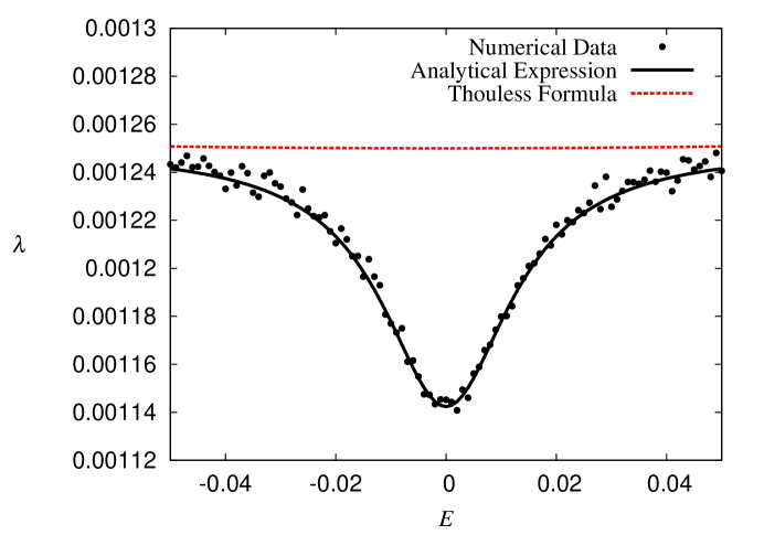
Figure 1: Inverse localisation length $\lambda$ versus $E$ in a neighbourhood of the band centre for uncorrelated disorder. The points correspond to the numerical data; the solid line to Eq. (65); the dashed line to Thouless’ formula. The data were obtained for $\sigma^{2}=10^{-2}$.

At the band centre, the invariant distribution (57) and the inverse localisation length (62) assume the well-known forms [20]

$$\rho(\theta,\varkappa=0)=\frac{1}{\mathbf{K}(1/\sqrt{2})}\frac{1}{\sqrt{3+\cos(4\theta)}},$$ (66)

and

$$\lambda(\varkappa=0)=\frac{\sigma^{2}}{4}\left[2\frac{\mathbf{E}\left(1/\sqrt{2}\right)}{\mathbf{K}\left(1/\sqrt{2}\right)}-1\right]=\sigma^{2}\left[\frac{\Gamma\left(3/4\right)}{\Gamma\left(1/4\right)}\right]^{2}.$$ (67)

In conclusion, the general expressions (55) and (60) reproduce the correct results in the limit case of uncorrelated disorder.

6 Disorder with exponentially decaying, positive correlations

In this section and in those that follow we consider the Anderson model (1) with correlated site energies. Sequences of random variables $\{\varepsilon_{n}\}$ with arbitrary binary correlations can be generated with the usual technique of filtering sequences of uncorrelated random variables [10].

We now focus our attention on the case of random site energies with positive spatial correlations that decay exponentially with the distance between sites. The key result is that the band-centre anomaly is quickly suppressed for increasing values of the correlation length, as first observed in [17]. As for the localisation length, it increases linearly with the correlation length, $l_{\mathrm{loc}}\propto l_{c}$.

We consider a binary correlator (4) of the form

$$\chi_{1}(l)=e^{-|l|/l_{c}}.$$ (68)

The corresponding power spectrum (19) is

$$W_{1}(x)=\sum_{l=-\infty}^{\infty}\chi(l)e^{i2lx}=\frac{\sinh(1/l_{c})}{\cosh(1/l_{c})-\cos(2x)}.$$ (69)

The behaviour of the power spectrum (69) is represented in Fig. 2 for various values of the correlation length.

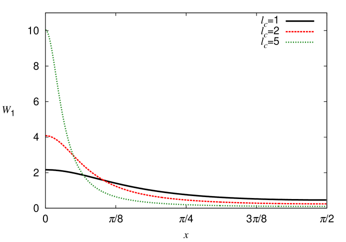
Figure 2: Power spectrum (69) versus $x$ for various values of the correlations length.

The values of the power spectrum (69) at the boundaries of its domain are

$$W_{1}(0)=\frac{1}{W_{1}(\pi/2)}=\frac{\sinh(1/l_{c})}{\cosh(1/l_{c})-1}.$$ (70)

Note that $W_{1}(0)$ and $W_{1}(\pi/2)$ are, respectively, an increasing and a decreasing function of $l_{c}$.

The invariant distribution for the angle variable is obtained by substituting the values (70) in the general expression (55). The analytical prediction matches well the numerical results, as can be seen in Figs. 3 and 4.

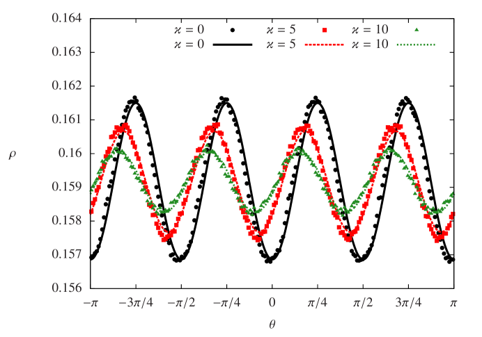
Figure 3: Invariant distribution $\rho(\theta,\varkappa)$ for various values of $\varkappa$. The disorder exhibits positive exponential correlations of the form (68) with $l_{c}=2$. Lines correspond to the theoretical formula (55); points to the numerical data. The numerical data were obtained for $\sigma^{2}=10^{-3}$.

Fig. 3 shows how the resonance effect is progressively reduced as the energy moves away from the band centre. This effect is expected and is found also in the case of uncorrelated disorder [21].

More surprising is the decrease of the modulation of the invariant measure (55) with the correlation length. The suppression of the band-centre anomaly as $l_{c}$ is increased is particularly evident at the band-centre, where the invariant distribution (57) takes the form

$$\rho(\theta,\varkappa=0)=\frac{1}{\displaystyle\mathbf{K}\left(\sqrt{\varphi_{-}(l_{c})/2}\right)}\frac{1}{\displaystyle\sqrt{4-\varphi_{-}(l_{c})\left[1-\cos\left(4\theta\right)\right]}}$$ (71)

with

$$\varphi_{-}(l_{c})=1-\frac{1}{\cosh\left(1/l_{c}\right)}.$$

For $l_{c}\to 0$, expression (71) differs from the corresponding formula (66) for uncorrelated disorder by exponentially small terms of order $O(e^{-1/l_{c}})$. As $l_{c}$ increases, however, the modulation of $\rho$ diminishes quickly, as shown by Fig. 4.

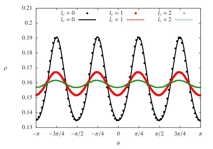
Figure 4: Invariant distribution $\rho(\theta,\varkappa=0)$ at the band centre for various values of the correlation length $l_{c}$. The disorder exhibits positive exponential correlations of the form (68). The lines correspond to the theoretical formula (71); the points to the numerical data. The data were obtained for $\sigma^{2}=10^{-3}$.

To understand this effect, it is useful to observe that, for $l_{c}\gg 1$, expression (71) reduces to

$$\rho(\theta,\varkappa=0)=\frac{1}{2\pi}\left[1-\frac{1}{16l_{c}^{2}}\cos\left(4\theta\right)+\ldots\right].$$ (72)

The asymptotic form (72) matches relatively well the numerical data already for values of $l_{c}\gtrsim 10$, as shown by Fig. 5.

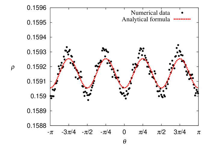
Figure 5: Invariant distribution $\rho(\theta,\varkappa=0)$ at the band centre for disorder with correlations of the form (68) with $l_{c}=10$. The line corresponds to the asymptotic formula (72); the points to the numerical data. The data were obtained for $\sigma^{2}=10^{-3}$.

The inverse localisation length can be computed with the help of Eqs. (55) and (60), supplemented by the specific values (70) of the power spectrum. In Fig. 6 we compare the numerically computed Lyapunov exponent with the theoretical expression (60) and with the formula (21) obtained by Izrailev and Krokhin.

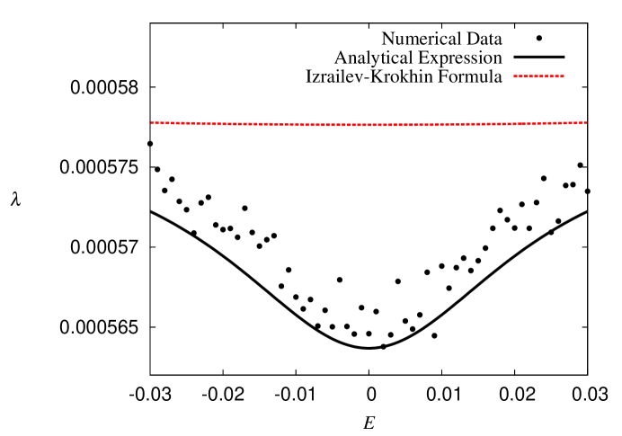
Figure 6: Inverse localisation length $\lambda$ versus $E$ in a neighbourhood of the band centre for disorder with correlations of the form (68) and $l_{c}=1$. The points correspond to the numerical data; the solid line to Eq. (60); the dashed line to the formula (21). The numerical data were obtained for $\sigma^{2}=10^{-2}$.

Note that the differences between the numerical values of $\lambda$ and the values predicted by Eq. (60) are of order $\sim 10^{-5}$, well within the $O(\sigma^{4})$ error intrinsic to the second-order approximation used in the theoretical calculations.

At the exact band centre, a relatively simple analytical expression for the inverse localisation length can be obtained by substituting the values (70) in Eq. (62). One obtains

$$\lambda(\varkappa=0)=\frac{\sigma^{2}}{4\sinh\left(1/l_{c}\right)}\left\{2\cosh\left(1/l_{c}\right)\frac{\displaystyle\mathbf{E}\left(\sqrt{\varphi_{-}(l_{c})/2}\right)}{\displaystyle\mathbf{K}\left(\sqrt{\varphi_{-}(l_{c})/2}\right)}-\cosh\left(1/l_{c}\right)-1\right\}.$$ (73)

Note that, for $l_{c}\gg 1$, the inverse localisation length (73) becomes

$$\lambda(\varkappa=0)\simeq\frac{\sigma^{2}}{16l_{c}}.$$

Therefore the extension of the band-centre state increases linearly with the correlation length $l_{c}$.

7 Exponentially decaying correlations with oscillating sign

We now consider correlations which decay exponentially with the distance between sites, but whose sign oscillates. Contrary to the previous case, the anomaly is now reinforced as the correlation length $l_{c}$ increases.

Mathematically, the correlations of the site energies have the form

$$\chi_{2}(l)=(-1)^{l}e^{-|l|/l_{c}}.$$ (74)

The corresponding power spectrum is

$$W_{2}(x)=\sum_{l=-\infty}^{\infty}\chi(l)e^{i2lx}=\frac{\sinh(1/l_{c})}{\cosh(1/l_{c})+\cos(2x)}.$$ (75)

The behaviour of the power spectrum (75) is represented in Fig. 7.

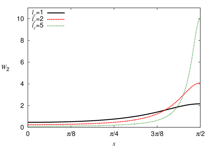
Figure 7: Power spectrum (75) versus $x$ for various values of the correlations length.

Eq. (75) implies that

$$W_{2}(0)=\frac{1}{W_{2}(\pi/2)}=\frac{\sinh(1/l_{c})}{\cosh(1/l_{c})+1}.$$ (76)

Note that

$$W_{2}\left(x\right)=W_{1}\left(\frac{\pi}{2}-x\right)$$

and that, therefore, the formulae for the invariant distribution and the inverse localisation length for this case can be obtained from the expressions for the previous case with the exchanges $W_{1}(0)\leftrightarrow W_{2}(\pi/2)$ and $W_{1}(\pi/2)\leftrightarrow W_{2}(0)$.

As before, the invariant distribution for the angle variable is obtained by substituting the specific values (76) of $W(0)$ and $W(\pi/2)$ in the general expression (55). The resulting analytical formula is corroborated by the numerical results, as shown by Figs. 8 and 9.

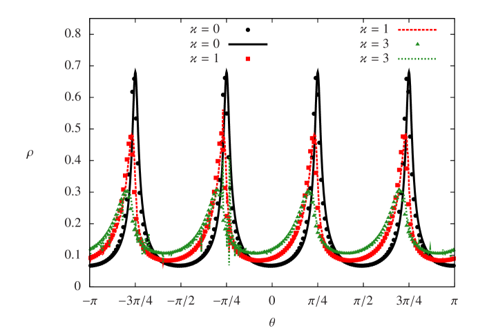
Figure 8: Invariant distribution $\rho(\theta,\varkappa)$ for various values of the parameter $\varkappa$. The lines correspond to the theoretical formula (55); the points to the numerical data. The data were obtained for disorder with correlation of the form (74) with $l_{c}=5$. The disorder strength in numerical calculations was $\sigma^{2}=10^{-3}$.

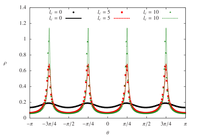
Figure 9: Invariant distribution $\rho(\theta,\varkappa=0)$ at the band centre for various values of the correlation length $l_{c}$. The disorder exhibits correlations of the form (74). The lines correspond to the theoretical formula (77); the points to the numerical data. The data were obtained for $\sigma^{2}=10^{-3}$.

Fig. 8 shows how correlation of the form (74) produce a strong modulation of the invariant measure at the band centre which is gradually reduced as the energy moves away from the band centre.

Fig. 9, on the other hand, shows how the invariant distribution develops conspicuous peaks as $l_{c}$ is increased. This behaviour is entirely consistent with the theoretical predictions. At the band centre, in fact, the general expression (57) for the invariant distribution takes the form

$$\rho(\theta,\varkappa=0)=\frac{1}{\displaystyle\mathbf{K}\left(\sqrt{\varphi_{+}(l_{c})/2}\right)}\frac{1}{\displaystyle\sqrt{4-\varphi_{+}(l_{c})\left[1-\cos\left(4\theta\right)\right]}}$$ (77)

with

$$\varphi_{+}(l_{c})=1+\frac{1}{\cosh(1/l_{c})}.$$

The asymptotic behaviour of the distribution (77) for $l_{c}\gg 1$ is

$$\rho(\theta,\varkappa=0)\simeq\frac{1}{\displaystyle 2^{3/2}\mathbf{K}\left(\sqrt{1-\frac{1}{4l_{c}^{2}}}\right)}\frac{1}{\displaystyle\sqrt{1+\frac{1}{4l_{c}^{2}}+\left(1-\frac{1}{4l_{c}^{2}}\right)\cos\left(4\theta\right)}}.$$ (78)

Note that for

$$\begin{array}[]{ccc}\displaystyle\theta\simeq\frac{\pi}{4}+n\frac{\pi}{2}&\mbox{ with }&n\in\mathbf{Z}\end{array}$$

the distribution (78) assumes the value

$$\rho\left(\frac{\pi}{4},\varkappa=0\right)\simeq\frac{l_{c}}{\displaystyle 2\mathbf{K}\left(\sqrt{1-\frac{1}{l_{c}^{2}}}\right)}$$

which diverges for $l_{c}\gg 1$. This entails that the distribution (77) develops four sharp maxima as $l_{c}$ is increased, in agreement with the data of Fig. 9.

After inserting the values (76) in the expression (55) for the invariant distribution, one can evaluate the rhs of Eq. (60) and obtain the inverse localisation length. The results agree with the numerical data, as shown by Fig. 10.

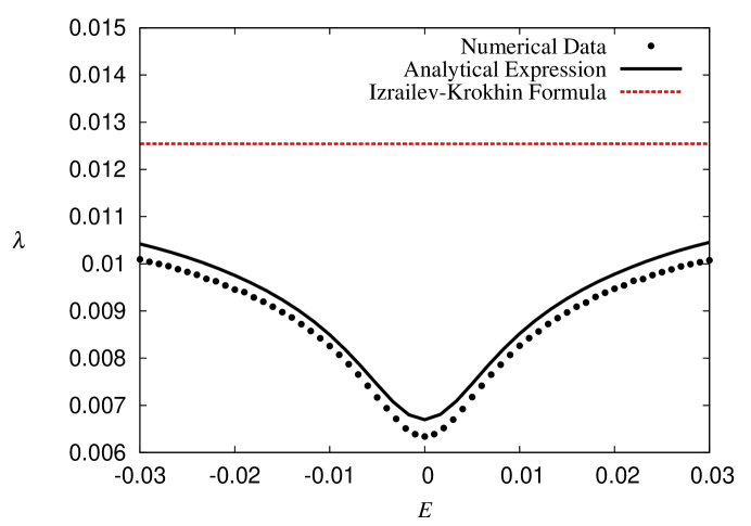
Figure 10: Inverse localisation length $\lambda$ versus $E$ in a neighbourhood of the band centre for disorder with correlations of the form (74) with $l_{c}=5$. The points correspond to the numerical data; the solid line to Eq. (60); the dashed line to the formula (21). The numerical data were obtained for $\sigma^{2}=10^{-2}$.

The slight discrepancy between numerical data and the theoretical expression is of order $O(\sigma^{4})$ and should probably be attributed to the neglected fourth-order correction in Eq. (60). Fig. 10 graphically shows that correlations of the form (74) increase the relative deviation of the Lyapunov exponent from the value predicted by the formula (21) obtained by Izrailev and Krokhin. This is consistent with the very large peaks that the invariant distribution develops in the present case.

Correlations of the form (74) have also the effect of enhancing the localisation of the electronic states for increasing values of the correlation length. This is a consequence of the fact that the factor $W(\pi/2)$, defined by Eq. (76), is an increasing function of $l_{c}$. This conclusion is confirmed by the explicit formula for the inverse localisation length at the exact band centre. For $E=0$, Eq. (62) becomes

$$\lambda(\varkappa=0)=\frac{\sigma^{2}}{4\sinh\left(1/l_{c}\right)}\left\{2\cosh\left(1/l_{c}\right)\frac{\displaystyle\mathbf{E}\left(\sqrt{\varphi_{+}(l_{c})/2}\right)}{\displaystyle\mathbf{K}\left(\sqrt{\varphi_{+}(l_{c})/2}\right)}-\cosh\left(1/l_{c}\right)+1\right\}.$$ (79)

As in the previous case, in the limit $l_{c}\to 0$ Eq. (79) differs from its counterpart (67) only by vanishing terms of order $O(e^{-1/l_{c}})$. In the limit $l_{c}\gg 1$, on the other hand, the inverse localisation length (79) diverges as

$$\lambda(\varkappa=0)=\frac{\sigma^{2}}{4}\left[\frac{2l_{c}}{\ln(8l_{c})}-\frac{1}{2l_{c}}+\ldots\right].$$

In this case the band-centre state becomes strongly localised as $l_{c}$ increases.

8 The case of a composite lattice

We now consider the case of a 1D chain with random energies whose binary correlator satisfies the condition

$$\begin{array}[]{ccc}\chi(2l+1)=0&\mbox{ for }&l\in\mathbf{Z}.\end{array}$$ (80)

A sequence $\{\varepsilon_{n}\}$ with correlations of the form (80) can be obtained by mixing two independent random sequences $\{\alpha_{n}\}$ and $\{\beta_{n}\}$ with the same statistical properties. More precisely, one assumes that

$$\langle\alpha_{n}\rangle=\langle\beta_{n}\rangle=0$$

and that the binary correlators are

$$\begin{array}[]{ccc}\langle\alpha_{n}\alpha_{n+l}\rangle=\langle\beta_{n}\beta_{n+l}\rangle=\sigma^{2}\tilde{\chi}(l)&\mbox{ and }&\langle\alpha_{n}\beta_{m}\rangle=0,\end{array}$$

where $\tilde{\chi}(l)$ is an arbitrary function, satisfying the condition that is quickly decays for $l\gg l_{c}$. One can then define the random energies by setting

$$\begin{array}[]{ccc}\varepsilon_{2n}=\alpha_{n}&\mbox{ and }&\varepsilon_{2n+1}=\beta_{n}.\end{array}$$

In physical terms, the chain is split in two independent and interpenetrating sublattices.

Condition (80) implies that the power spectrum must satisfy the identity

$$W(0)=W\left(\frac{\pi}{2}\right).$$

As a consequence, the invariant distribution (55) assumes the particularly simple form

$$\begin{array}[]{ccl}\rho(\theta,\varkappa)&=&\displaystyle\frac{1}{N(\tilde{\varkappa})}\frac{e^{-8\tilde{\varkappa}F_{0}(\theta)}}{\sqrt{3+\cos(4\theta)}}\left[e^{4\sqrt{2}\pi\tilde{\varkappa}}\int_{0}^{\theta}\frac{e^{8\tilde{\varkappa}F_{0}(\phi)}}{\sqrt{3+\cos(4\phi)}}\mathrm{d}\phi\right.\\ &+&\displaystyle\left.\int_{\theta}^{2\pi}\frac{e^{8\tilde{\varkappa}F_{0}(\phi)}}{\sqrt{3+\cos(4\phi)}}\mathrm{d}\phi\right],\end{array}$$ (81)

where $N$ is a normalisation constant, $F_{0}(\theta)$ is defined by Eq. (64), and

$$\tilde{\varkappa}=\frac{\varkappa}{W(0)}.$$ (82)

The distribution (81) has the same form of the distribution (63) for uncorrelated disorder, the only difference being that the parameter (50) of the latter is replaced by the rescaled parameter (82) in the former. In physical terms, this means that the correlations do not modify the modulation of $\rho$, but they alter the scale over which the distance of the energy from the band centre is measured. This entails that the anomaly extends over a larger energy interval if $W(0)>1$ and is restricted to a shrunken region if $W(0)<1$.

At the exact band centre, $\tilde{\varkappa}=\varkappa=0$ and the invariant distribution reduces to the form (66). Correspondingly, the inverse localisation length becomes

$$\lambda(\varkappa=0)=\frac{\sigma^{2}}{4}\left[2\frac{\mathbf{E}\left(1/\sqrt{2}\right)}{\mathbf{K}\left(1/\sqrt{2}\right)}-1\right]W\left(\frac{\pi}{2}\right).$$ (83)

8.1 Long-ranged correlations

We now focus our attention on a specific type of correlator fulfilling condition (80), i.e.,

$$\chi_{3}(l)=\frac{1+(-1)^{l}}{2}\frac{\sin\left(2al\right)}{2al},$$ (84)

where the parameter $a$ lies in the interval $[0,\pi/4]$. The correlator (84) does not decreases quickly for $l\gtrsim l_{c}$, and therefore does not satisfy one of the conditions used to derive our analytical results. It can be fitted in our theoretical framework, however, if it considered as the limit form for $l_{c}\to\infty$ of the correlator

$$\chi_{3}(l)=\frac{1+(-1)^{l}}{2}\frac{\sin\left(2al\right)}{2al}\exp\left(-\frac{|l|}{l_{c}}\right).$$ (85)

The power spectrum of this correlator is

$$\begin{array}[]{ccl}W_{3}(x)&=&\displaystyle 1+\frac{1}{4a}\left\{\arctan\left[\frac{\sin\left(2a+2x\right)}{e^{1/l_{c}}-\cos\left(2a+2x\right)}\right]-\arctan\left[\frac{\sin\left(2a+2x\right)}{e^{1/l_{c}}+\cos\left(2a+2x\right)}\right]\right.\\ &+&\displaystyle\left.\arctan\left[\frac{\sin\left(2a-2x\right)}{e^{1/l_{c}}-\cos\left(2a-2x\right)}\right]-\arctan\left[\frac{\sin\left(2a-2x\right)}{e^{1/l_{c}}+\cos\left(2a-2x\right)}\right]\right\}.\\ \end{array}$$ (86)

In the limit $l_{c}\to\infty$ the power spectrum (86) tends to the form

$$W_{3}(x)=\left\{\begin{array}[]{ccl}\displaystyle\frac{\pi}{4a}&\mbox{if}&\displaystyle x\in\left[0,a\right]\cup\left[\frac{\pi}{2}-a,\frac{\pi}{2}\right]\\ 0&\mbox{if}&\displaystyle x\in\left[a,\frac{\pi}{2}-a\right]\\ \end{array}.\right.$$ (87)

The behaviour of the power spectrum (86) with $a=\pi/10$ is represented in Fig. 11 for various values of $l_{c}$.

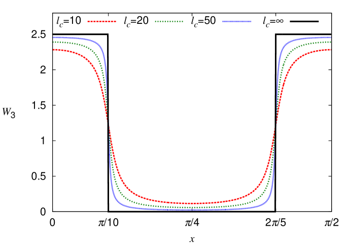
Figure 11: Power spectrum (86) with $a=\pi/10$ for various values of the correlations length. For $l_{c}\to\infty$, mobility edges appear at $x_{1}=\pi/10$ and $x_{2}=2\pi/5$.

In the limit $l_{c}\to\infty$, the power spectrum vanishes for $x_{1}=\pi/10<x<x_{2}=2\pi/2$; according to the standard formula (21), this generates mobility edges at $E_{1}\simeq\pm 0.618$ and $E_{2}\simeq\pm 1.902$.

When the binary correlator takes the form (85), the invariant distribution is given by the expression (81). This is true for any finite value of the correlation length; under the reasonable assumption that $\rho(\theta,\varkappa)$ should be a continuous function of $l_{c}$, one can conclude that the invariant distribution keeps the form (81) even in the limit $l_{c}\to\infty$, i.e., when the binary correlator is given by Eq. (84). The numerical data corroborate this conclusion, as shown by Fig. 12.

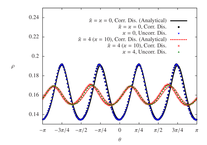
Figure 12: Invariant distribution $\rho(\theta,\tilde{\varkappa})$ for disorder with correlations of the form (84) with $a=\pi/10$. The data correspond to the values $\tilde{\varkappa}=0$ (band centre) and $\tilde{\varkappa}=4$. Lines correspond to the theoretical formula (81); points to the numerical data. Also represented are the numerical data for the invariant distributions for uncorrelated disorder and values $\varkappa=0$ and $\varkappa=4$ of the parameter (50). In numerical computations the disorder strength was set at $\sigma^{2}=10^{-2}$.

As can be seen, the numerical data match well the theoretical distribution (81) both at the band centre ($\tilde{\varkappa}=0$) and away from it ($\tilde{\varkappa}=4$). In Fig. 12 we also plot the numerically obtained invariant distributions for uncorrelated disorder with $\varkappa=0$ (band centre) and $\varkappa=4$. The data show that, as expected, these two distributions collapse on the distributions for correlated disorder with $\tilde{\varkappa}=0$ and $\tilde{\varkappa}=4$. Note that in the present case value $W(0)=5/2$ so that $\varkappa=10$ when $\tilde{\varkappa}=4$.

We can now consider the behaviour of the localisation length. In Fig. 13 we plot the Lyapunov exponent as a function of the energy. One can easily see that the formula (21) proposed by Izrailev and Krokhin agrees well with the numerical data; in particular, effective mobility edges arise where expected. Discrepancies between the numerical data and the expression (21) appear at the band centre and at the band edges, however, where anomalies occur.

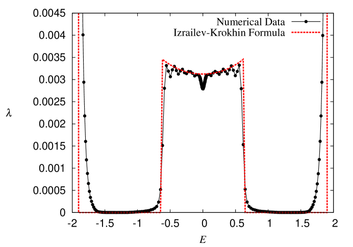
Figure 13: Inverse localisation length $\lambda$ versus $E$ for disorder with correlations of the form (84). The points correspond to numerical data; the dashed line to the standard formula (21). The data were obtained for $\sigma^{2}=10^{-2}$.

The band-centre anomaly is represented in greater detail in Fig. 14, where we compare the numerical data with the standard formula (21) and with Eq. (59). The use of the expression (59), rather then (60), is due to the fact that in this case the anomaly extends, as predicted, over a larger energy interval and, therefore, the term $\cos^{2}(\delta)$ in Eq. (59) cannot be approximated with unity as done so far.

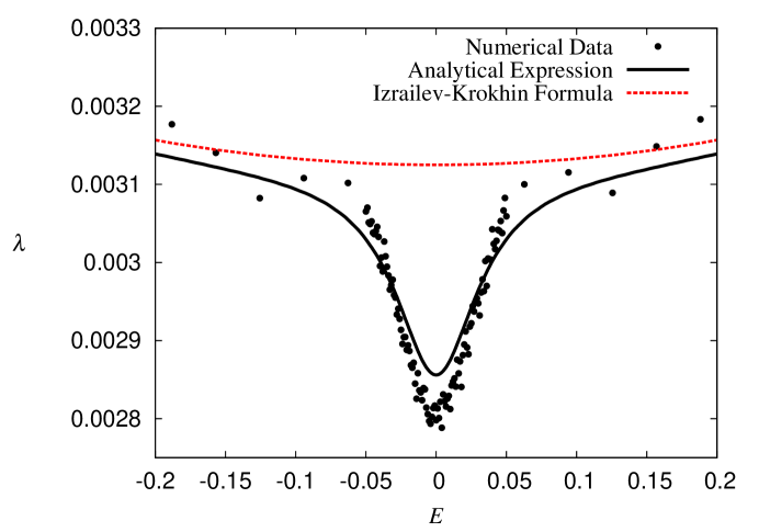
Figure 14: Inverse localisation length $\lambda$ versus $E$ in a neighbourhood of the band centre for disorder with correlations of the form (84). The points correspond to the numerical data; the solid line to Eq. (59); the dashed line to the standard formula (21). The data were obtained for $\sigma^{2}=10^{-2}$.

Fig. 14 confirms that our theoretical results work rather well even for long-ranged correlations of the form (84). The extension of the energy interval with anomalous behaviour can be clearly seen if one compares the data represented in Fig. 14 with those corresponding to uncorrelated disorder shown in Fig. 1.

To conclude the discussion of long-ranged correlations, we can consider the case of disorder with correlations of the form

$$\chi_{4}(l)=\frac{\sin\left(2al\right)}{\left(2al\right)}\cos\left(\frac{\pi}{2}l\right)\exp\left(-\frac{|l|}{l_{c}}\right).$$ (88)

The limit form for $l_{c}\to\infty$ is

$$\chi_{4}(l)=\frac{\sin\left(2al\right)}{\left(2al\right)}\cos\left(\frac{\pi}{2}l\right).$$

The power spectrum corresponding to the correlator (88) is

$$\begin{array}[]{ccl}W_{4}(x)&=&\displaystyle 1+\frac{1}{4a}\left\{\arctan\left[\frac{e^{1/l_{c}}+\sin\left(2x-2a\right)}{\cos\left(2x-2a\right)}\right]+\arctan\left[\frac{e^{1/l_{c}}-\sin\left(2x+2a\right)}{\cos\left(2x+2a\right)}\right]\right.\\ &&\displaystyle\left.-\arctan\left[\frac{e^{1/l_{c}}+\sin\left(2x+2a\right)}{\cos\left(2x+2a\right)}\right]-\arctan\left[\frac{e^{1/l_{c}}-\sin\left(2x-2a\right)}{\cos\left(2x-2a\right)}\right]\right\}.\\ \end{array}$$ (89)

In the limit $l_{c}\to\infty$ the power spectrum (89) tends to the form

$$W_{4}(x)=\left\{\begin{array}[]{ccl}\displaystyle\frac{\pi}{\pi-4a}&\mbox{if}&\displaystyle x\in\left[\frac{\pi}{4}-a,\frac{\pi}{4}+a\right]\\ 0&\mbox{if}&\displaystyle x\in\left[0,\frac{\pi}{4}-a\right]\cup\left[\frac{\pi}{4}+a,\frac{\pi}{2}\right]\\ \end{array}.\right.$$

We thus obtain a power spectrum which is complementary with respect to the case described by Eq. (87). The behaviour of the power spectrum (89) with $a=\pi/10$ is represented in Fig. 15 for various values of $l_{c}$.

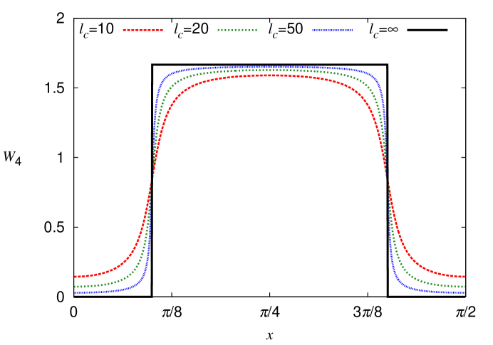
Figure 15: Power spectrum (89) with $a=\pi/10$ for various values of the correlations length. As $l_{c}\to\infty$, mobility edges arise at $x_{1}=\pi/10$ and $x_{2}=2\pi/5$.

As can be seen from Eq. (89), for increasing values of $l_{c}$ the power spectrum tends to zero at the boundaries of the domain $[0,\pi/2]$. This entails that the anomaly at the band centre becomes unstable as $l_{c}\to\infty$. In fact, although at the exact band centre the invariant distribution keeps the form (66), the fact that $W(0)=W(\pi/2)\to 0$ implies that the rescaled parameter (82) grows very quickly for any infinitesimal deviation of the energy from the band centre. Therefore the invariant distribution becomes uniform very fast when the energy moves away from the band centre.

We can conclude that, depending on the value of the power spectrum at the band centre, correlations satisfying condition (80) can either strengthen or weaken the band centre anomaly. They do not enhance or suppress the modulation of the invariant distribution, but they can widen or shrink the neighbourhood of the band centre where the invariant distribution is significantly non-uniform.

9 Conclusions

In this paper we have studied the band-centre anomaly in the 1D Anderson model with weak correlated disorder. Our perturbative analysis used two essential tools: the Hamiltonian map approach and the continuum limit. The Hamiltonian map approach interprets the spatial structure of the electronic states in terms of the time evolution of a classical parametric oscillator. The dynamical evolution of the angle variable of this oscillator is dictated by the random map (23). Replacing this map with a corresponding stochastic differential equation is a crucial step that allowed us to derive our analytical results and that required the elaboration of the specific integration scheme (34). We obtained analytical expressions for the invariant distribution of the phase variable and for the localisation length. These results are valid for weak disorder with arbitrary correlations and generalise the formulae obtained in [21] for the case of uncorrelated disorder.

When disorder is uncorrelated, the invariant distribution of the phase variable, which is uniform for non-resonant values of the energy, becomes modulated for energies lying in a neighbourhood of the band centre. This modulation, in turn, generates a deviation of the inverse localisation length from the values predicted by Thouless’ formula. In qualitative terms, this picture holds also when disorder displays spatial correlations. From a quantitative point of view, however, the size and extension of the resonance effect can be dramatically altered. Two extreme cases are discussed in Sec. 6 and 7. In the first case, the site energies exhibit positive correlations which decay exponentially with the distance between sites. In this case the resonance effect is suppressed upon increasing the correlation length $l_{c}$. In the second case, the correlations between site energies also decrease exponentially in magnitude, but oscillate between positive and negative values. In this case, increasing the correlation length $l_{c}$ strongly enhances the modulation of the invariant measure, which tends to a sum of four delta peaks for $l_{c}\gg 1$. Correspondingly, the difference between the inverse localisation length and the value predicted by the formula derived by Izrailev and Krokhin increases with $l_{c}$. The specific long-range correlations analysed in Sec. 8 do not alter the modulation of the invariant distribution with respect to the case of uncorrelated disorder, but can strengthen or weaken the anomaly in a different way, i.e., they can enlarge or restrict the interval of the energy in which the resonant effect is relevant.

In conclusion, we have shown that correlations of the disorder can alter the band-centre anomaly very strongly and in a variety of ways. In particular, specific correlations can suppress or magnify the resonance effect at the centre of the energy band.

References

- [1] P. W. Anderson, Phys. Rev. 109, 1492 (1958)
- [2] P. A. Lee, T. V. Ramakrishnan, Rev. Mod. Phys. 57, 287 (1985)
- [3] C. W. J. Beenakker, Rev. Mod. Phys. 69, 731 (1997)
- [4] D. J. Thouless, p.1 in “La matière mal condensée - Ill-Condensed Matter”, R. Balian, R. Maynard, G. Toulouse eds., North-Holland (Amsterdam) and World Scientific (Singapore), 1979
- [5] G. Czycholl, B. Kramer, A. MacKinnon, Z. Phys. B 43, 5 (1981)
- [6] M. Kappus, F. Wegner, Z. Phys. B 45, 15 (1981)
- [7] B. Derrida, E. Gardner, J. Physique 45, 1283 (1984)
- [8] R. Kuske, Z. Scuss, I. Goldhirsch, S. H. Noskowicz, SIAM J. Appl. Math. 53, 1210 (1993)
- [9] I. Goldhirsch, S. H. Noskowicz, Z. Schuss, Phys. Rev. B 49, 14504 (1994)
- [10] F. M. Izrailev, A. A. Krokhin, N. M. Makharov, Phys. Rep. 512, 125 (2012)
- [11] E. Abrahams, P. W. Anderson, D. C. Licciardello, T. V. Ramakrishnan, Phys. Rev. Lett. 42, 673 (1979)
- [12] P. W. Anderson, D. J. Thouless, E. Abrahams, D. S. Fischer, Phys. Rev. B, 22, 3519 (1980)
- [13] A. D. Stone, D. C. Allan, J. D. Joannopoulos, Phys. Rev. B 27, 836 (1983)
- [14] H. Schomerus, M. Titov, Phys. Rev. B 67, 100201(R) (2003)
- [15] L. I. Deych, A. A. Lisyansky, B. L. Altshuler, Phys. Rev. Lett. 84, 2678 (2000); L. I. Deych, M. V. Erementchouk, A. A. Lisyansky, B. L. Altshuler, Phys. Rev. Lett. 91, 096601 (2003); J. Heinrichs, J. Phys. C: Condens. Matter, 16, 7995 (2004)
- [16] M. Titov, H. Schomerus, Phys. Rev. Lett. 95, 126602 (2005)
- [17] I. F. Herrera-González, F. M. Izrailev, N. M. Makarov, L. Tessieri, Suppression of the band center anomaly in the one-dimensional Anderson model with short-range correlated disorder, in preparation.
- [18] F. M. Izrailev, T. Kottos, G. Tsironis, Phys. Rev. B 52, 3274 (1995)
- [19] F. M. Izrailev, A. A. Krokhin, Phys. Rev. Lett., 82, 4062 (1999)
- [20] F. M. Izrailev, S. Ruffo, L. Tessieri, J. Phys. A: Math. Gen., 31, 5263 (1998)
- [21] L. Tessieri, I. F. Herrera-González, F. M. Izrailev, Physica E, 44, 1260 (2012)
- [22] G. H. Hardy, E. M. Wright, An Introduction to the Theory of Numbers, 4th ed., Oxford University Press, Oxford (1960)
- [23] P. E. Kloeden, E. Platen, Numerical Solution of Stochastic Differential Equations, Springer, Berlin (1992)
- [24] R. F. Fox, J. Math. Phys., 18, 2331 (1977); N. G. Van Kampen, J. Stat. Phys., 54, 1289 (1989); J. Casademunt, J. M. Sancho, Phys. Rev. A, 39, 4915 (1989)
- [25] N. G. Van Kampen, Stochastic Processes in Physics and Chemistry, 3rd ed., North Holland, Amsterdam (2007)
- [26] R. Mannella, V. Palleschi, Phys. Rev. A, 40, 3381 (1989); G. N. Milshtein, M. V. Tret’yakov, J. Stat. Phys., 77, 691 (1994)
- [27] L. Tessieri, F. M. Izrailev, Phys. Rev. E, 64, 066120 (2001)
- [28] R. Mannella, Int. J. Mod. Phys. C, 13, 1177 (2002)