Where to look for natural supersymmetry

Abstract

Why is natural supersymmetry neither detected nor ruled-out to date? To answer this question we use the Bayesian approach where the emphasis in finding prior-independent features within broader and minimally biased frames is taken as the guiding principle. The 20-parameter minimal supersymmetric standard model (MSSM) global fits to subjective naturalness indicate the existence of a prior-independent upper bound on the pseudoscalar Higgs boson mass $m_{A}$ as a function of $\tan\beta$, the ratio of the vacuum expectation values of MSSM Higgs doublets. For a 30-parameter MSSM this implies that $m_{A}\lesssim 3\>\text{TeV}$ and $\tan\beta\lesssim 25$ at 95% Bayesian confidence. Removing the contradictory subjectiveness within the electroweak fine-tuning measure leads to finding the naturalness line, $m_{A}\sim\frac{1}{\sqrt{2}}\,m_{Z}\,\tan\beta,$ that reduces by one the number of MSSM Higgs sector free parameters.

Introduction:

Supersymmetry Martin:1997ns model constructions and phenomenological studies go decades back Wess:1974tw ; Fayet:1976et ; Fayet:1977yc ; Dimopoulos:1981zb ; Nilles:1983ge ; Haber:1984rc ; Barbieri:1982eh ; Dawson:1983fw but yet have not been discovered nor ruled out by high-energy physics experiments. The specific prediction from supersymmetry is that there must be new, beyond the standard model, particles with and without colour charges. But it does not specify what the particular masses and couplings of the new particles will be. These remain arbitrary with more than 100 free parameters. Currently, on the experiments side, it is expected that the large hadron collider (LHC) will give a definite answer as to whether low-energy supersymmetry has any role in stabilising the Higgs boson mass at $125\>\text{GeV}$ Aad:2012tfa ; Chatrchyan:2012ufa ; Aad:2015zhl . It is going to probe the so-called “natural” supersymmetry. In view of this we ask the question: Is there any robust prediction from natural supersymmetry that could be targeted by the experiments for a discovery or an absolute exclusion? We are going to address this question by employing Bayesian statistical techniques. The Bayesian method can be used to extract robust predictions from a model based on experimental data. Here the model under consideration will be the R-parity conserving minimal supersymmetric standard model (MSSM).

Robust predictions can be extracted because the Bayesian approach allows a check for the stability of results with respect to widely different but well-motivated changes in the prior assumptions concerning the base supersymmetry parameters. The results which remain the same under the change of the prior assumptions are said to be prior-independent and represent the predictions by the model based on the experimental data. Before the LHC commissioning, the 20-parameter MSSM fits AbdusSalam:2008uv ; AbdusSalam:2009qd to neutralino cold dark matter (CDM) relic density, electroweak and B-physics data revealed two observables to be prior-independent, namely the (then undiscovered) Higgs boson and the lightest top-squark masses. The Higgs boson mass was predicted to lie between 119 and 128 GeV within the 95% Bayesian credibility region, while the top-squark mass to be around $2\>\text{TeV}$. The 20-parameter MSSM is specified by

$$\underline{\theta}=\{M_{1,2,3};\;\;m^{3rd\,gen}_{\tilde{f}_{Q,U,D,L,E}},\;\;m^{1st/2nd\,gen}_{\tilde{f}_{Q,U,D,L,E}};\;\;A_{t,b,\tau,\mu=e},\;\;m^{2}_{H_{u,d}},\;\;\tan\beta;\;\;m_{Z},\;\;m_{t},\;\;m_{b},\;\;\alpha_{em}^{-1},\;\;\alpha_{s}\}$$ (1)

where the gaugino mass parameters $M_{1}$, $M_{2}$ and $M_{3}$ were allowed in -4 to 4 TeV range. The sfermion $\tilde{f}$ mass parameters $m_{\tilde{f}}$ vary between 100 GeV to 4 TeV. The trilinear scalar couplings $A_{t,b,\tau,\mu=e}\in[-8,8]$ TeV. The Higgs-sector parameters $m^{2}_{H_{u}}$, $m^{2}_{H_{d}}$, were varied according to $m^{2}\in sign(m)\,[-4,4]^{2}\textrm{TeV}^{2}$. The ratio of the vacuum expectation values $\tan\beta=\left<H_{u}\right>/\left<H_{d}\right>$ is allowed to be between 2 and 60, while $sign(\mu)$ the sign of the Higgs doublets mixing parameter, is allowed to be randomly $\pm 1$. The remaining five standard model parameters were also varied in a Gaussian manner with central values and deviations according to experimental results pdg .

In this article we are going to show that by imposing fine-tuning cuts within the 20-parameters MSSM, an additional prior-independent result manifests. From this, an inequality relation between the pseudoscalar Higgs boson mass $m_{A}$ and $\tan\beta$ can be deduced. For the cuts we use the electroweak fine-tuning measure Baer:2012up ; Baer:2012cf $\Delta_{EW}$ defined as follows. Consider the electroweak symmetry breaking condition for a 1-loop corrected Higgs potential, $V+\Delta V$

$$\frac{m_{Z}^{2}}{2}=\frac{m_{H_{d}}^{2}+\Sigma_{d}^{d}-(m_{H_{u}}^{2}+\Sigma_{u}^{u})\tan^{2}\beta}{\tan^{2}\beta-1}-\mu^{2}.$$ (2)

Here $\Sigma_{u}^{u}$ and $\Sigma_{d}^{d}$ arise from the 1-loop radiative corrections. For naturalness, each term in the right hand side of Eq. 2 should be comparable to $m^{2}_{Z}/2$ so that

$$\Delta_{EW}\equiv max_{i}\left(C_{i}\right)/(m_{Z}^{2}/2)$$ (3)

accommodates the fact that for obtaining a natural value of $m_{Z}$ then the terms $C_{i}$, with $i=H_{d},\ H_{u}$, $\mu$, $\Sigma_{u}^{u}(k)$, $\Sigma_{d}^{d}(k)$, where $k$ denotes the various particles and sparticles contributions, must be of order $m_{Z}^{2}/2$. Using the terms that couple the most to the Higgs sector (the case $k=\tilde{t}_{1,2},\tilde{b}_{1,2}$) we have

$$\begin{split}C_{\mu}&=|-\mu^{2}|,\\ C_{H_{u}}&=|-m_{H_{u}}^{2}\tan^{2}\beta/(\tan^{2}\beta-1)|,\,\\ C_{H_{d}}&=|m_{H_{d}}^{2}/(\tan^{2}\beta-1)|,\\ C_{\Sigma^{d}_{d}}&=|\Sigma^{d}_{d}/(\tan^{2}\beta-1)|,\\ C_{\Sigma^{u}_{u}}&=|-\Sigma^{u}_{u}\,\tan^{2}\beta/(\tan^{2}\beta-1)|,\\ \Sigma^{d,u}_{d,u}&=\Sigma_{i}\,|\Sigma^{d,u}_{d,u}(i)|.\end{split}$$ (4)

The expressions for $\Sigma^{d,u}_{d,u}(i)$ are shown in the Appendix.

In the next section, we describe the Bayesian approach to MSSM naturalness, the fitting procedure and the prior-independent result obtained. After that we explain the impact of the result which is a prior-independent bound on $m_{A}$ as a function of $\tan\beta$ on the a 30-parameters MSSM posterior distribution. We then assess to what extent has some relevant 8 TeV LHC supersymmetry limits probe the natural MSSM-30. At the end, we present an analytical argument that exposes a subtle methodological contradiction by looking closer at the electroweak fine-tuning measure. Fixing the contradiction lead to a no fine-tuning “naturalness line”. After this we summarise our results and give an outlook for future studies.

Naturalness, the Bayesian approaches:

There are two major trends in the literature concerning Bayesian approach to MSSM naturalness. First, for addressing MSSM naturalness one can compute the amount of fine-tuning at each point during the parameters sampling and then penalise highly fine-tuned points according to a chosen subjective limit (see e.g. Allanach:2006jc ). Within this method, various groups use different fine-tuning measures, e.g. Harnik:2003rs ; Kitano:2005wc ; Ellis:1986yg ; Barbieri:1987fn . The difference measures, however, agree when used appropriately as explained in Baer:2014ica ; Baer:2013gva . According to the second trend, fine-tuning measures manifest implicitly within the Bayesian global fit procedures. In Cabrera:2008tj ; Ghilencea:2012qk ; Fowlie:2014xha it is shown that fitting the MSSM parameters in a Bayesian way automatically incorporate a fine-tuning penalisation. Our approach in this article goes along the first trend. We use the electroweak fine-tuning measure Eq. 3 and penalise or rule-out MSSM points with $\Delta_{EW}>4$. The choice $\Delta_{EW}>4$ in search for prior-independent results from global fits to MSSM represents the “naturalness” data. A natural MSSM point should have $\Delta_{EW}\rightarrow 1.$ Relaxing away from $\Delta_{EW}=1$ as a fine-tuning cut we choose $\Delta_{EW}<2+2$ where the first “2” represents a 50% fine-tuning and the second a 100% “theoretical” allowance on the first. The Bayesian global fit procedure with $\Delta_{EW}\leq 4$ is described as follows.

Fitting procedure:

Based on the methodology for our MSSM programme Feroz:2008wr ; AbdusSalam:2008uv ; AbdusSalam:2009qd ; AbdusSalam:2009tr ; AbdusSalam:2010qp ; AbdusSalam:2011hd ; AbdusSalam:2012sy ; AbdusSalam:2012ir ; AbdusSalam:2013qba the Bayesian global fit of the 20-parameters MSSM plus 5 standard model parameters (MSSM-25) were performed separately with linear and logarithmic prior probability distributions on the parameters Eq. 1. These were fit to the Higgs boson mass, naturalness requirement, neutralino CDM relic density, electroweak and B-physics data shown in Tab. 1.

Observable	Constraint	Observable	Constraint
$m_{W}$ [GeV]	$80.399\pm 0.027$ verzo	$A^{l}=A^{e}$	$0.1513\pm 0.0021$ :2005ema
$\Gamma_{Z}$ [GeV]	$2.4952\pm 0.0025$ :2005ema	$A^{b}$	$0.923\pm 0.020$ :2005ema
$\sin^{2}\,\theta_{eff}^{lep}$	$0.2324\pm 0.0012$ :2005ema	$A^{c}$	$0.670\pm 0.027$ :2005ema
$\delta a_{\mu}$	$(30.2\pm 9.0)\times 10^{10}$ Bennett:2006fi ; Davier:2007ua	$Br(B\rightarrow X_{s}\gamma)$	$(3.55\pm 0.42)\times 10^{4}$ Barberio:2007cr
$R_{l}^{0}$	$20.767\pm 0.025$ :2005ema	$Br(B_{s}\rightarrow\mu^{+}\mu^{-})$	$3.2^{+1.5}_{-1.2}\times 10^{-9}$ Aaij:2012nna
$R_{b}^{0}$	$0.21629\pm 0.00066$ :2005ema	$R_{\Delta M_{B_{s}}}$	$0.85\pm 0.11$Abulencia:2006ze
$R_{c}^{0}$	$0.1721\pm 0.0030$ :2005ema	$R_{Br(B_{u}\rightarrow\tau\nu)}$	$1.26\pm 0.41$ Aubert:2004kz ; paoti ; hep-lat/0507015
$A_{\textrm{FB}}^{b}$	$0.0992\pm 0.0016$ :2005ema	$\Delta_{0-}$	$0.0375\pm 0.0289$J.Phys.G33.1
$A_{\textrm{FB}}^{c}$	$0.0707\pm 0.035$ :2005ema	$\Omega_{CDM}h^{2}$	$0.11\pm 0.02$ 0803.0547
		$m_{h}$	$125.6\pm 3.0$ [GeV]ATLAS:2013mma ; CMS:yva

Table 1: Summary for the central values and errors for the Higgs boson mass, the electroweak physics observables, B-physics observables and cold dark matter relic density constraints.

MultiNest Feroz:2007kg ; Feroz:2008xx package which implements nested sampling algorithm Skilling for exploring model parameters space were used. At each MSSM-25 point the supersymmetry spectra were computed via SOFTSUSY Allanach:2001kg and the list of observables $O_{i}$,

$$\begin{split}\underline{O}=&\{m_{W},\;\sin^{2}\,\theta^{lep}_{eff},\;\Gamma_{Z},\;\delta a_{\mu},\;R_{l}^{0},\;A_{fb}^{0,l},\;A^{l}=A^{e},\;R_{b,c}^{0},\;A_{fb}^{b,c},\;A^{b,c},\;BR(B\rightarrow X_{s}\,\gamma),\;\\ &BR(B_{s}\rightarrow\mu^{+}\,\mu^{-}),\;\Delta_{0-},\;R_{BR(B_{u}\rightarrow\tau\nu)},\;R_{\Delta M_{B_{s}}},\Omega_{CDM}h^{2},\;m_{h},\,\Delta_{EW}^{-1}\geq 5\%\,\},\end{split}$$ (5)

via the following packages. micrOMEGAs Belanger:2008sj was used for computing neutralino CDM relic density $\Omega_{CDM}h^{2}$ and the anomalous magnetic moment of the muon $\delta a_{\mu}$; and SuperIso Mahmoudi:2007vz for predicting $BR(B_{s}\rightarrow\mu^{+}\mu^{-})$, $BR(B\rightarrow s\gamma)$ and the isospin asymmetry, $\Delta_{0-}$, in $B\rightarrow K^{*}\gamma$. With susyPOPE Heinemeyer:2006px ; Heinemeyer:2007bw we computed the $W$-boson mass $m_{W}$, the effective leptonic mixing angle variable $\sin^{2}\theta^{lep}_{eff}$, the total $Z$-boson decay width, $\Gamma_{Z}$, and the other electroweak observables. These allow the computation of the posterior probability via Bayes’ theorem,

$$p(\underline{\theta}|\underline{d},{\cal{H}})=L_{\Delta_{EW}}\,L_{CDM}(x)\prod_{i}\,\frac{e^{\left[-(O_{i}-\mu_{i})^{2}/2\sigma_{i}^{2}\right]}}{\sqrt{2\pi\sigma_{i}^{2}}}\,\frac{p(\underline{\theta}|{\cal{H}})}{p(\underline{d}|{\cal{H}})};$$ (6)

$$L_{\Delta_{EW}}=\begin{cases}1,&\textrm{if $\Delta_{EW}^{-1}\geq 50\%$}\\ 0,&\textrm{if $\Delta_{EW}^{-1}<50\%$}\\ \end{cases},\quad L_{CDM}(x)=\begin{cases}1/(y+\sqrt{\pi s^{2}/2}),&\textrm{if $x<y$}\\ e^{\left[-(x-y)^{2}/2s^{2}\right]}/(y+\sqrt{\pi s^{2}/2}),&\textrm{if $x\geq y$}\\ \end{cases}.$$ (7)

Here $i$ run over the different experimental observables (data) other than the CDM relic density, $x$ represents the predicted value of the neutralino CDM relic density, $y=0.11$ is the WMAP central value quoted in Tab. 1 and $s=0.02$ the inflated error. The likelihood contribution coming from the CDM relic density is given by $L_{CDM}(x)$ which is purely Gaussian when the predicted relic density $x$ is greater than the experimental central value $y=0.11$ thus imposing penalisation for CDM over-production. No penalisation is imposed when $x<y$. The set of experimental data used for the fits is

$$\underline{d}=d_{Tab.~{}\ref{tab:obs}}+d_{\Delta_{EW}}=\{\mu_{i},\sigma_{i}\}+\{\Delta_{EW}^{-1}>50\%\}.$$ (8)

Here $d_{Tab.~{}\ref{tab:obs}}$ is the set of experimental central values $\mu_{i}$ and error $\sigma_{i}$ shown in Tab. 1. ${\cal H}$ in Eq. 6 represents the context or hypothesis for the Bayesian theorem. i.e. nature is supersymmetric and that neutralinos make part of the cold dark matter relics. From the posterior of the global fits we only show the result which is approximately prior-independent. This happens to be an MSSM-25 feature in the $(m_{A},\,\tan\beta)$ plane.

Result:

The two-dimensional posterior distributions in Fig. 1 shows that requiring fine-tuning no worse than 50% as naturalness data while fitting the MSSM-25 to data has a prior-independent impact in the $(m_{A},\tan\beta)$ plane. The empty triangular regions are excluded by this naturalness requirement. The prior-independent result is

$$m_{A}<\,\frac{4}{30}\,\tan\beta\,\>\text{TeV}.$$ (9)

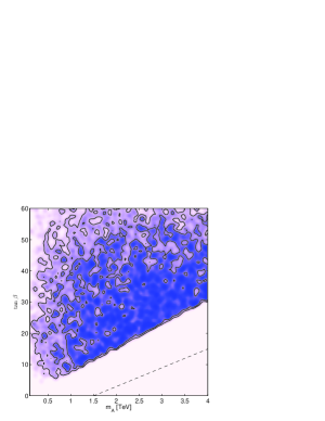
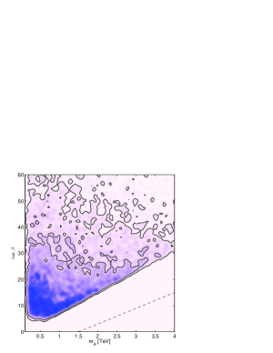
Figure 1: Two-dimensional posterior distributions from the MSSM-25 fits to experimental plus “naturalness” data. The left-side (right-side) plot is for logarithmic (flat) prior fit. The empty triangular region on the plots are explicitly excluded by the naturalness limit $\Delta_{EW}\leq 4$. The dashed line represents the shift that will occur when a relaxed naturalness cut $\Delta_{EW}\leq 20$ is imposed. The solid contour lines enclose the dark blue (dark) and light violet (light grey to white) regions which correspond respectively to the 68% and 95% Bayesian credibility. For both panels dark blue (dark) regions have higher probability compared to the light blue to light violate (grey to white) ones.

Eq. 9 is robust and can be applied to any supersymmetry model with a necessary electroweak symmetry breaking condition Eq. 2. Next, we assess the impact of this on the posterior sample of an MSSM-30 which favours low values of $\tan\beta\lesssim 27$ within 95% Bayesian credibility. First we give a brief introduction of the MSSM-30 frame and then afterwards check the natural (Eq. 9-based) MSSM-30 points against some LHC supersymmetry limits.

Naturalness constraint on MSSM-30:

In AbdusSalam:2014uea , the 30-parameters MSSM was constructed by reducing the parent 100+ MSSM parameters using a systematic treatment of minimal flavour violation – unlike as done by hand for the MSSM-25 case. The parameters consist of $e^{\phi_{1}}M_{1}$, $e^{\phi_{2}}M_{2}$, and $M_{3}$ in the gaugino sector with $M_{1,\,2}$ (and also their imaginary parts $Im(M_{1,\,2})$) which are varied between -4 to 4 TeV. $M_{3}$ is allowed to be between 100 GeV to 4 TeV. Within the Higgs sector, $m_{A}$ is varied between $100\>\text{GeV}$ to $4\>\text{TeV}$ while $\mu$ and $Im(\mu)$ were allowed within -4 to 4 TeV. As for MSSM-25, $\tan\beta$ is allowed to be between 2 and 60. The scalar mass and trilinear coupling parameters are $\displaystyle M^{2}_{Q}=\tilde{a}_{1}+x_{1}X_{13}+y_{1}X_{1},\quad M^{2}_{E}=\tilde{a}_{7}+y_{7}X_{1},$ $\displaystyle M^{2}_{U}=\tilde{a}_{2}+x_{2}X_{1},\quad A_{E}=\tilde{a}_{8}X_{1},$ $\displaystyle M^{2}_{D}=\tilde{a}_{3}+y_{3}X_{1},\quad A_{U}=\tilde{a}_{4}X_{5}+y_{4}X_{1},$ $\displaystyle M^{2}_{L}=\tilde{a}_{6}+y_{6}X_{1},\quad A_{D}=\tilde{a}_{5}X_{1}+y_{5}X_{5},$ $\displaystyle\begin{array}[]{cccc}X_{1}=\delta_{3i}\delta_{3j},&X_{2}=\delta_{2i}\delta_{2j},&X_{3}=\delta_{3i}\delta_{2j},&X_{4}=\delta_{2i}\delta_{3j},\\ X_{5}=\delta_{3i}V_{3j},&X_{6}=\delta_{2i}V_{2j},&X_{7}=\delta_{3i}V_{2j},&X_{8}=\delta_{2i}V_{3j},\\ X_{9}=V^{*}_{3i}\delta_{3j},&X_{10}=V^{*}_{2i}\delta_{2j},&X_{11}=V^{*}_{3i}\delta_{2j},&X_{12}=V^{*}_{2i}\delta_{3j},\\ X_{13}=V^{*}_{3i}V_{3j},&X_{14}=V^{*}_{2i}V_{2j},&X_{15}=V^{*}_{3i}V_{2j},&X_{16}=V^{*}_{2i}V_{3j}.\\ \end{array}$ (14)

The bases $X_{1,\ldots,16}$ are products amongst Kronecker delta $\delta$ and the Cabibbo-Kobayashi-Maskawa mixing matrix $V$ elements. The parameters $\tilde{a}_{1,2,3,6,7}>0$ and $x_{1,2},y_{1,3,6,7}$ were varied within $(100\>\text{GeV})^{2}$ to $(4\>\text{TeV})^{2}$ and $-(4\>\text{TeV})^{2}$ to $(4\>\text{TeV})^{2}$ respectively; while $\tilde{a}_{4,5,8}$, $Im(\tilde{a}_{4,5,8})$, $y_{4,5}$ and $Im(y_{4,5})$ were allowed between $-8\>\text{TeV}$ to $8\>\text{TeV}$. The SM parameters are fixed according to experimental results as: mass of the Z-boson, $m_{Z}=91.2\>\text{GeV}$, top quark mass, $m_{t}=173.2\>\text{GeV}$, bottom quark mass, $m_{b}=4.2\>\text{GeV}$, the electromagnetic coupling, $\alpha_{em}^{-1}=127.9$, and the strong interaction coupling, $\alpha_{s}=0.119$. The parameters are

$$\underline{\theta}\equiv\{\,M_{1,2,3},\,\quad\mu,\,\quad m_{A},\,\quad\tan\beta,\,\quad Im(M_{1,2},\,\quad\mu),\,\quad\tilde{a}_{1,2,\ldots,8},Im(\tilde{a}_{4,5,8}),\,\quad x_{1,2},\,\quad y_{1,3,4,5,6,7},\,\quad Im(y_{4,5})\,\}.$$ (15)

The MSSM-30 fits to the Higgs boson mass, the electroweak physics, B-physics, lepton dipole moments and the cold dark matter relic density observables disfavour large $\tan\beta\gtrsim 30$. The corresponding posterior distribution on $(m_{A},\tan\beta)$ plane is show in Fig. 2(a). The $(m_{A},\tan\beta)$ plane is chosen because we aim at showing the impact of the prior-independent result Eq. 9 on the MSSM-30 posterior sample. Fig. 2(b) shows what remains after imposing the prior-independent naturalness condition Eq. 9 by ruling out the unnatural points. From the surviving posterior, it is deduced that $m_{A}\lesssim 3\>\text{TeV}$ and $\tan\beta\lesssim 25$ at 95% Bayesian credibility.

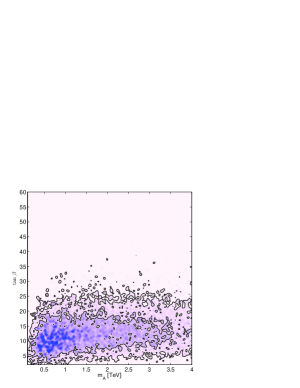
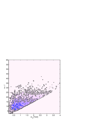
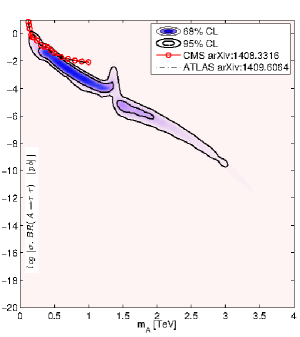
(a)  (b)  (c)  (d) 

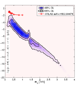
Figure 2: (a) The posterior distribution for the MSSM-30 on ($m_{A}$, $\tan\beta$) plane. (b) Explicitly shows the effect of the naturalness cut Eq. 9 on the MSSM-30 posterior sample. Note that small patches of regions that show up in (b) but absent in the parent plot (a) is an artifact of colouring and contouring interpolations/normalisation. (c) and (d) show the effect of the ATLAS and CMS 95% upper bounds on the production cross-section times decay branching ratios for the MSSM-30 pseudoscalar Higgs boson. For all the panels dark blue (dark) regions have higher probability compared to the light blue to light violate (grey to white) ones.

Collider limits on natural MSSM-30 points:

To what extent does 8 TeV LHC probe the natural MSSM-30 posterior point based on Fig. 9? The natural points can be checked against some LHC limits. ATLAS and CMS 95% confidence level limits can be used to constrain models that predict the processes they searched for. Limits on fiducial cross sections usually call for writing Rivet Buckley:2010ar analyses to pass over Herwig++ Bahr:2008pv Monte Carlo generated supersymmetry events. We did not intend to use the full set of such LHC results. Rather, a selected few which are relevant for probing the prior-independent naturalness condition Eq. 9 were considered. In Aad:2014ioa a search for scalar particles decaying via narrow resonances into two photons is performed. The limits applied on the MSSM-30 pseudoscalar Higgs production cross section times branching ratio into two photons did not significantly constrain the posterior sample. The ATLAS Aad:2014vgg and CMS Khachatryan:2014wca limits from search for MSSM Higgs bosons (here the pseudoscalar Higgs) decaying into tau-lepton pairs were also considered. These are put next to the production cross section times branching fraction of the pseudoscalar decay into tau-leptons for the MSSM-30 posterior computed using FeynHiggsHeinemeyer:1998yj . Fig. 2(d) shows the similar case for the ATLAS search for a CP-odd Higgs boson decaying to the Z-boson and the SM Higgs boson which in turn decays to tau-leptons Aad:2015wra . All these searches hardly constrain the natural MSSM-30 posterior mostly due to the low production cross-section and decay rates of the pseudoscalar Higgs at the LHC. Perhaps, searches with topologies involving the pseudoscalar MSSM Higgs boson decaying via charginos and neutralinos could probe better the naturalness allowed MSSM-30 region.

Naturalness line:

Here we give a closer look at the numerical and prior-independent result Eq. 9. A zeroth-order explanation for the bound on $m_{A}$ as function of $\tan\beta$ can be explained using the electroweak fine-tuning measure $\Delta_{EW}$ Baer:2012up ; Bae:2014fsa . Consider the electroweak symmetry breaking condition, assuming $\tan\beta>>1$ but without lost of generality

$$\frac{1}{2}m_{Z}^{2}\approx\frac{m_{H_{d}}^{2}}{\tan^{2}\beta}-m_{H_{u}}^{2}-\mu^{2}.$$ (16)

Requiring there be no fine-tuning will need all three terms on the right hand side to be comparable amongst themselves and of order $m_{Z}^{2}/2$. As such $\frac{m^{2}_{H_{d}}}{\tan^{2}\beta}\sim m_{Z}^{2}/2$ and $-m^{2}_{H_{u}}-\mu^{2}\sim 0$ implies that $m^{2}_{H_{u}}\sim-\mu^{2}$. In addition $(\frac{m^{2}_{H_{d}}}{\tan^{2}\beta})/(-m^{2}_{H_{u}})\sim 1$ implies $m^{2}_{H_{d}}>>-m^{2}_{H_{u}}$. Now applying $m^{2}_{H_{u}}\sim-\mu^{2}$ and $m^{2}_{H_{d}}>>-m^{2}_{H_{u}}$ to the the tree-level relation $m_{A}^{2}=2|\mu|^{2}+m_{H_{d}}^{2}+m_{H_{u}}^{2}$ gives $m_{A}^{2}\sim m_{H_{d}}^{2}.$ Therefore requiring fine-tuning $\Delta_{EW}$ no worst that $\Delta_{max}$

$$\Delta_{EW}\equiv\frac{2\,m_{H_{d}}^{2}}{m_{Z}^{2}\,\tan^{2}\beta}\leq\Delta_{max}\quad\implies\quad m_{A}<m_{Z}\,\tan\beta\,(\Delta_{max}/2)^{1/2}.$$ (17)

Loop corrections to the tree-level relation for $m_{A}^{2}$ is not going spoil the bound Eq. 17 or Eq. 9. This is the case for the loop-corrected Carena:2002es $m_{A}$ used for the MSSM-25 fits as can be seen in Fig. 1. There is also no conflict with other fine-tuning measures Harnik:2003rs ; Kitano:2005wc ; Ellis:1986yg ; Barbieri:1987fn since all the measures agree with one another whenever appropriately applied Baer:2014ica ; Baer:2013gva . As such the core message of this letter goes as follows. We seek for robust predictions for assessing low-energy supersymmetry as the model responsible for the Higgs boson mass stability. But this is not possible as long as the subjectiveness inherent in the fine-tuning measure Eq. 17 remains. Constructing the bound in Eq. 17 is based on the no fine-tuning and comparability requirements for the terms in Eq. 16. Now imposing $\Delta_{EW}\leq\Delta_{max}$ is a contradiction since this allows fine-tuning even if not worse than $1/\Delta_{max}$. Fig. 1 give further insight to this. The fits done with $\Delta_{max}=20$ shows the corresponding no-go regions similar to the case with $\Delta_{max}=4$ which do not agree with Eq. 17. Our take is that a model point is either fine-tuned, meaning $\Delta_{EW}>1$ or not fine-tuned when $\Delta_{EW}=1.$ This way the subjectiveness in selecting a cut on fine-tuning is completely removed. The out come of this is a robust “naturalness line”

$$m_{A}\sim\frac{1}{\sqrt{2}}\,m_{Z}\,\tan\beta.$$ (18)

In fact imposing Eq. 18 reduces the $(m_{A},\tan\beta)$ plane into a line, meaning one less parameter in the Higgs sector. Note that this result is not equivalent with the purely tree-level no fine-tuning measure $\mu\sim\frac{1}{\sqrt{2}}\,m_{Z}$. The ansatz is that the naturalness line holds at all loop levels such that radiative corrections to the masses do not spoil the relation. The naturalness line Eq. 18 can be used for mapping natural regions of any MSSM frame.

Conclusions and outlook:

We have addressed a question about finding an objective determinant for the existence of natural supersymmetry. Our Bayesian approach is based on finding prior-independent features within broader and minimally biased frames as the guiding principle susy2013 . The results of this article and an outlook are summarised as follows.

• The 20-parameter MSSM fits to subjective naturalness, using the electroweak fine-tuning measure, indicate the existence of a prior-independent upper bound on the pseudoscalar Higgs boson mass $m_{A}$ as a function of $\tan\beta.$ Imposing the bound on the posterior sample of a 30-parameter MSSM fit to data shows that $m_{A}\lesssim 3\>\text{TeV}$ and $\tan\beta\lesssim 25$ at 95% Bayesian credibility region. The natural MSSM-30 points are not yet ruled out by the 8 TeV LHC limits we considered. Constraints from search topologies that include decays into charginos and neutralinos could lead to better probe.

• We seek for robust predictions for assessing low-energy supersymmetry as the model responsible for the Higgs boson mass stability. We proposed that this is possible only if the subjectiveness inherent in the electroweak fine-tuning measure is removed. Imposing $\Delta_{EW}\leq\Delta_{max}$ is a contradiction since this allows fine-tuning even if not worse than $1/\Delta_{max}$. A robust method should require their either be fine-tuning, meaning $\Delta_{EW}>1$ or no fine-tuning, i.e. $\Delta_{EW}=1.$ This way the subjectiveness in selecting a cut on fine-tuning is completely removed and no fine-tuning means $m_{A}\sim\frac{1}{\sqrt{2}}\,m_{Z}\,\tan\beta.$ We call this relation the “naturalness line”.

• “Why is supersymmetry not yet discovered?” Up to the public LHC results as of the time of writing this article, we claim that an answer is that the regions where it is expected are not yet probed. “Where to look for natural supersymmetry?” The proposed regions where it should be expected were derived via Bayesian method with minimal model framework construction or theoretical prejudice. Natural supersymmetry should be looked for along the “naturalness line” $m_{A}\sim\frac{1}{\sqrt{2}}\,m_{Z}\,\tan\beta$ together with a 1-2 TeV lightest top-squarks. The 8 TeV LHC limits on gluino and 1st-2nd generation sparticles are not in conflict with these predictions.

• An interesting line for further studies will be to assess the impact of the full set of LHC fiducial cross section limits on the “naturalness line” in general and within particular phenomenological frames such as the 30-parameters MSSM AbdusSalam:2014uea of the 2-parameters hMSSM Djouadi:2013uqa .

Appendix: The expressions for the $\Sigma_{u}^{u}(\tilde{t}_{1,2},\tilde{b}_{1,2})$ contributions to $\Delta_{EW}$

For self-sufficiency we explicitly show the expressions for $\Sigma_{u}^{u}(\tilde{t}_{1,2},\tilde{b}_{1,2})$ according to Arnowitt:1992qp ; Gladyshev:1996fx

$$\Sigma_{u}^{u}(\tilde{t}_{1,2})=\frac{3}{16\pi^{2}}\,F(m_{\tilde{t}_{1,2}}^{2})\times\left[f_{t}^{2}-g_{Z}^{2}\mp\frac{f_{t}^{2}A_{t}^{2}-8g_{Z}^{2}(\frac{1}{4}-\frac{2}{3}x_{W})\Delta_{t}}{m_{\tilde{t}_{2}}^{2}-m_{\tilde{t}_{1}}^{2}}\right]\textrm{ and }$$ (19)

$$\Sigma_{d}^{d}(\tilde{t}_{1,2})=\frac{3}{16\pi^{2}}\,F(m_{\tilde{t}_{1,2}}^{2})\left[g_{Z}^{2}\mp\frac{f_{t}^{2}\mu^{2}+8g_{Z}^{2}(\frac{1}{4}-\frac{2}{3}x_{W})\Delta_{t}}{m_{\tilde{t}_{2}}^{2}-m_{\tilde{t}_{1}}^{2}}\right]$$ (20)

where $\Delta_{t}=(m_{\tilde{t}_{L}}^{2}-m_{\tilde{t}_{R}}^{2})/2+M_{Z}^{2}\,\cos 2\beta(\frac{1}{4}-\frac{2}{3}x_{W})$, $g_{Z}^{2}=(g^{2}+g^{\prime 2})/8$, $x_{W}\equiv\sin^{2}\theta_{W}$ and $F(m^{2})=m^{2}\left(\log(m^{2}/Q^{2})-1\right)$, with $Q^{2}=m_{\tilde{t}_{1}}m_{\tilde{t}_{2}}$. $m_{\tilde{t}_{1,2}}$ are computed at tree-level. For the bottom-squarks,

$$\Sigma_{u}^{u}(\tilde{b}_{1,2})=\frac{3}{16\pi^{2}}\,F(m_{\tilde{b}_{1,2}}^{2})\left[g_{Z}^{2}\mp\frac{f_{b}^{2}\mu^{2}-8g_{Z}^{2}(\frac{1}{4}-\frac{1}{3}x_{W})\Delta_{b}}{m_{\tilde{b}_{2}}^{2}-m_{\tilde{b}_{1}}^{2}}\right]\textrm{ and }$$ (21)

$$\Sigma_{d}^{d}(\tilde{b}_{1,2})=\frac{3}{16\pi^{2}}\,F(m_{\tilde{b}_{1,2}}^{2})\left[f_{b}^{2}-g_{Z}^{2}\mp\frac{f_{b}^{2}A_{b}^{2}-8g_{Z}^{2}(\frac{1}{4}-\frac{1}{3}x_{W})\Delta_{b}}{m_{\tilde{b}_{2}}^{2}-m_{\tilde{b}_{1}}^{2}}\right]$$ (22)

where $\Delta_{b}=(m_{\tilde{b}_{L}}^{2}-m_{\tilde{b}_{R}}^{2})/2+M_{Z}^{2}\,\cos 2\beta(\frac{1}{4}-\frac{1}{3}x_{W})$. $m_{\tilde{b}_{1,2}}$ are computed at tree-level.

References

- (1) S. P. Martin, “A Supersymmetry Primer,” arXiv:hep-ph/9709356.
- (2) J. Wess and B. Zumino, “Supergauge Transformations in Four-Dimensions,” Nucl. Phys. B70 (1974) 39–50.
- (3) P. Fayet, “Supersymmetry and Weak, Electromagnetic and Strong Interactions,” Phys. Lett. B64 (1976) 159.
- (4) P. Fayet, “Spontaneously Broken Supersymmetric Theories of Weak, Electromagnetic and Strong Interactions,” Phys. Lett. B69 (1977) 489.
- (5) S. Dimopoulos and H. Georgi, “Softly Broken Supersymmetry and SU(5),” Nucl. Phys. B193 (1981) 150–162.
- (6) H. P. Nilles, “Supersymmetry, Supergravity and Particle Physics,” Phys. Rept. 110 (1984) 1–162.
- (7) H. E. Haber and G. L. Kane, “The Search for Supersymmetry: Probing Physics Beyond the Standard Model,” Phys. Rept. 117 (1985) 75–263.
- (8) R. Barbieri, S. Ferrara, and C. A. Savoy, “Gauge Models with Spontaneously Broken Local Supersymmetry,” Phys. Lett. B119 (1982) 343.
- (9) S. Dawson, E. Eichten, and C. Quigg, “Search for Supersymmetric Particles in Hadron - Hadron Collisions,” Phys. Rev. D31 (1985) 1581.
- (10) ATLAS Collaboration, G. Aad et al., “Observation of a new particle in the search for the Standard Model Higgs boson with the ATLAS detector at the LHC,” Phys.Lett. B716 (2012) 1–29, arXiv:1207.7214 [hep-ex].
- (11) CMS Collaboration, S. Chatrchyan et al., “Observation of a new boson at a mass of 125 GeV with the CMS experiment at the LHC,” Phys.Lett. B716 (2012) 30–61, arXiv:1207.7235 [hep-ex].
- (12) ATLAS, CMS Collaboration, G. Aad et al., “Combined Measurement of the Higgs Boson Mass in Collisions at and 8 TeV with the ATLAS and CMS Experiments,” Phys. Rev. Lett. 114 (2015) 191803, arXiv:1503.07589 [hep-ex].
- (13) S. S. AbdusSalam, “The Full 24-Parameter MSSM Exploration,” AIP Conf. Proc. 1078 (2009) 297–299, arXiv:0809.0284 [hep-ph].
- (14) S. S. AbdusSalam, B. C. Allanach, F. Quevedo, F. Feroz, and M. Hobson, “Fitting the Phenomenological MSSM,” arXiv:0904.2548 [hep-ph].
- (15) Particle Data Group Collaboration, W. M. Yao et al., “Review of particle physics,” J. Phys. G33 (2006) 1–1232.
- (16) H. Baer, V. Barger, P. Huang, A. Mustafayev, and X. Tata, “Radiative natural SUSY with a 125 GeV Higgs boson,” Phys.Rev.Lett. 109 (2012) 161802, arXiv:1207.3343 [hep-ph].
- (17) H. Baer, V. Barger, P. Huang, D. Mickelson, A. Mustafayev, et al., “Radiative natural supersymmetry: Reconciling electroweak fine-tuning and the Higgs boson mass,” Phys.Rev. D87 (2013) 115028, arXiv:1212.2655 [hep-ph].
- (18) B. C. Allanach, “Naturalness priors and fits to the constrained minimal supersymmetric standard model,” Phys. Lett. B635 (2006) 123–130, arXiv:hep-ph/0601089.
- (19) R. Harnik, G. D. Kribs, D. T. Larson, and H. Murayama, “The Minimal supersymmetric fat Higgs model,” Phys. Rev. D70 (2004) 015002, arXiv:hep-ph/0311349 [hep-ph].
- (20) R. Kitano and Y. Nomura, “A solution to the supersymmetric fine-tuning problem within the MSSM,” Phys. Lett. B631 (2005) 58–67, arXiv:hep-ph/0509039.
- (21) J. R. Ellis, K. Enqvist, D. V. Nanopoulos, and F. Zwirner, “Observables in Low-Energy Superstring Models,” Mod. Phys. Lett. A1 (1986) 57.
- (22) R. Barbieri and G. F. Giudice, “Upper Bounds on Supersymmetric Particle Masses,” Nucl. Phys. B306 (1988) 63–76.
- (23) H. Baer, V. Barger, D. Mickelson, and M. Padeffke-Kirkland, “SUSY models under siege: LHC constraints and electroweak fine-tuning,” Phys. Rev. D89 no. 11, (2014) 115019, arXiv:1404.2277 [hep-ph].
- (24) H. Baer, V. Barger, and D. Mickelson, “How conventional measures overestimate electroweak fine-tuning in supersymmetric theory,” Phys. Rev. D88 no. 9, (2013) 095013, arXiv:1309.2984 [hep-ph].
- (25) M. E. Cabrera, J. A. Casas, and R. Ruiz de Austri, “Bayesian approach and Naturalness in MSSM analyses for the LHC,” JHEP 03 (2009) 075, arXiv:0812.0536 [hep-ph].
- (26) D. Ghilencea and G. Ross, “The fine-tuning cost of the likelihood in SUSY models,” Nucl.Phys. B868 (2013) 65–74, arXiv:1208.0837 [hep-ph].
- (27) A. Fowlie, “CMSSM, naturalness and the ”fine-tuning price” of the Very Large Hadron Collider,” Phys. Rev. D90 (2014) 015010, arXiv:1403.3407 [hep-ph].
- (28) F. Feroz et al., “Bayesian Selection of sign(mu) within mSUGRA in Global Fits Including WMAP5 Results,” JHEP 10 (2008) 064, arXiv:0807.4512 [hep-ph].
- (29) S. S. AbdusSalam, B. C. Allanach, M. J. Dolan, F. Feroz, and M. P. Hobson, “Selecting a Model of Supersymmetry Breaking Mediation,” arXiv:0906.0957 [hep-ph].
- (30) S. AbdusSalam and F. Quevedo, “Cold Dark Matter Hypotheses in the MSSM,” arXiv:1009.4308 [hep-ph].
- (31) S. AbdusSalam, “Can the LHC rule out the MSSM?,” Phys.Lett. B705 (2011) 331–336, arXiv:1106.2317 [hep-ph].
- (32) S. S. AbdusSalam and D. Choudhury, “Higgs boson discovery versus sparticles prediction: Impact on the pMSSM’s posterior samples from a Bayesian global fit,” arXiv:1210.3331 [hep-ph].
- (33) S. S. AbdusSalam, “LHC-7 supersymmetry search interpretation within the pMSSM,” Phys.Rev. D87 (2013) 115012, arXiv:1211.0999 [hep-ph].
- (34) S. S. AbdusSalam, “Stop-mass prediction in naturalness scenarios within MSSM-25,” Int. J. Mod. Phys. A29 no. 27, (2014) 1450160, arXiv:1312.7830 [hep-ph].
- (35) M. Verzocchi in talk at ICHEP 2008, Philadelphia, USA. 2008.
- (36) ALEPH Collaboration, “Precision electroweak measurements on the resonance,” Phys. Rept. 427 (2006) 257, arXiv:hep-ex/0509008.
- (37) Muon G-2 Collaboration, G. W. Bennett et al., “Final report of the muon E821 anomalous magnetic moment measurement at BNL,” Phys. Rev. D73 (2006) 072003, arXiv:hep-ex/0602035.
- (38) M. Davier, “The hadronic contribution to (g-2)(mu),” Nucl. Phys. Proc. Suppl. 169 (2007) 288–296, arXiv:hep-ph/0701163.
- (39) Heavy Flavor Averaging Group (HFAG) Collaboration, E. Barberio et al., “Averages of hadron properties at the end of 2006,” arXiv:0704.3575 [hep-ex].
- (40) LHCb Collaboration, R. Aaij et al., “First Evidence for the Decay ,” Phys.Rev.Lett. 110 (2013) 021801, arXiv:1211.2674 [hep-ex].
- (41) CDF Collaboration, A. Abulencia et al., “Observation of B/s0 anti-B/s0 oscillations,” Phys. Rev. Lett. 97 (2006) 242003, arXiv:hep-ex/0609040.
- (42) BABAR Collaboration, B. Aubert et al., “Search for the rare leptonic decay ,” Phys. Rev. Lett. 95 (2005) 041804, arXiv:hep-ex/0407038.
- (43) P. Chang in talk at ICHEP 2008, Philadelphia, USA. 2008.
- (44) HPQCD Collaboration, A. Gray et al., “The B Meson Decay Constant from Unquenched Lattice QCD,” Phys. Rev. Lett. 95 (2005) 212001, arXiv:hep-lat/0507015.
- (45) Particle Data Group Collaboration, C. Amsler et al., “Review of particle physics,” Phys. Lett. B667 (2008) 1.
- (46) WMAP Collaboration, E. Komatsu et al., “Five-Year Wilkinson Microwave Anisotropy Probe (WMAP) Observations:Cosmological Interpretation,” Astrophys. J. Suppl. 180 (2009) 330–376, arXiv:0803.0547 [astro-ph].
- (47) ATLAS Collaboration, “Combined measurements of the mass and signal strength of the Higgs-like boson with the ATLAS detector using up to 25 fb-1 of proton-proton collision data,” ATLAS-CONF-2013-014, ATLAS-COM-CONF-2013-025.
- (48) CMS Collaboration, “Combination of standard model Higgs boson searches and measurements of the properties of the new boson with a mass near 125 GeV,” CMS-PAS-HIG-13-005.
- (49) F. Feroz and M. P. Hobson, “Multimodal nested sampling: an efficient and robust alternative to MCMC methods for astronomical data analysis,” arXiv:0704.3704 [astro-ph].
- (50) F. Feroz, M. P. Hobson, and M. Bridges, “MultiNest: an efficient and robust Bayesian inference tool for cosmology and particle physics,” arXiv:0809.3437 [astro-ph].
- (51) J. Skilling, “Nested Sampling,” in American Institute of Physics Conference Series, R. Fischer, R. Preuss, and U. V. Toussaint, eds., pp. 395–405. Nov., 2004. http://www.inference.phy.cam.ac.uk/bayesys/.
- (52) B. C. Allanach, “SOFTSUSY: A C++ program for calculating supersymmetric spectra,” Comput. Phys. Commun. 143 (2002) 305–331, arXiv:hep-ph/0104145.
- (53) G. Belanger, F. Boudjema, A. Pukhov, and A. Semenov, “Dark matter direct detection rate in a generic model with micrOMEGAs2.1,” arXiv:0803.2360 [hep-ph].
- (54) F. Mahmoudi, “SuperIso: A program for calculating the isospin asymmetry of B -¿ K* gamma in the MSSM,” Comput. Phys. Commun. 178 (2008) 745–754, arXiv:0710.2067 [hep-ph].
- (55) S. Heinemeyer, W. Hollik, D. Stockinger, A. M. Weber, and G. Weiglein, “Precise prediction for M(W) in the MSSM,” JHEP 08 (2006) 052, arXiv:hep-ph/0604147.
- (56) S. Heinemeyer, W. Hollik, A. M. Weber, and G. Weiglein, “ Pole Observables in the MSSM,” JHEP 04 (2008) 039, arXiv:0710.2972 [hep-ph].
- (57) S. S. AbdusSalam, C. P. Burgess, and F. Quevedo, “MFV Reductions of MSSM Parameter Space,” JHEP 02 (2015) 073, arXiv:1411.1663 [hep-ph].
- (58) A. Buckley, J. Butterworth, L. Lonnblad, D. Grellscheid, H. Hoeth, J. Monk, H. Schulz, and F. Siegert, “Rivet user manual,” Comput. Phys. Commun. 184 (2013) 2803–2819, arXiv:1003.0694 [hep-ph].
- (59) M. Bahr et al., “Herwig++ Physics and Manual,” Eur. Phys. J. C58 (2008) 639–707, arXiv:0803.0883 [hep-ph].
- (60) ATLAS Collaboration, G. Aad et al., “Search for Scalar Diphoton Resonances in the Mass Range GeV with the ATLAS Detector in Collision Data at = 8 ,” Phys. Rev. Lett. 113 no. 17, (2014) 171801, arXiv:1407.6583 [hep-ex].
- (61) ATLAS Collaboration, G. Aad et al., “Search for neutral Higgs bosons of the minimal supersymmetric standard model in pp collisions at = 8 TeV with the ATLAS detector,” JHEP 11 (2014) 056, arXiv:1409.6064 [hep-ex].
- (62) CMS Collaboration, V. Khachatryan et al., “Search for neutral MSSM Higgs bosons decaying to a pair of tau leptons in pp collisions,” JHEP 10 (2014) 160, arXiv:1408.3316 [hep-ex].
- (63) S. Heinemeyer, W. Hollik, and G. Weiglein, “FeynHiggs: A Program for the calculation of the masses of the neutral CP even Higgs bosons in the MSSM,” Comput. Phys. Commun. 124 (2000) 76–89, arXiv:hep-ph/9812320 [hep-ph].
- (64) ATLAS Collaboration, G. Aad et al., “Search for a CP-odd Higgs boson decaying to Zh in pp collisions at TeV with the ATLAS detector,” Phys. Lett. B744 (2015) 163–183, arXiv:1502.04478 [hep-ex].
- (65) K. J. Bae, H. Baer, V. Barger, D. Mickelson, and M. Savoy, “Implications of naturalness for the heavy Higgs bosons of supersymmetry,” Phys. Rev. D90 no. 7, (2014) 075010, arXiv:1407.3853 [hep-ph].
- (66) M. Carena and H. E. Haber, “Higgs boson theory and phenomenology,” Prog. Part. Nucl. Phys. 50 (2003) 63–152, arXiv:hep-ph/0208209 [hep-ph].
- (67) S. S. AbdusSalam in Supersymmetry without prejudice, when? talk at SUSY 2013. 2013, Trieste.
- (68) A. Djouadi, L. Maiani, G. Moreau, A. Polosa, J. Quevillon, and V. Riquer, “The post-Higgs MSSM scenario: Habemus MSSM?,” Eur. Phys. J. C73 (2013) 2650, arXiv:1307.5205 [hep-ph].
- (69) R. L. Arnowitt and P. Nath, “Loop corrections to radiative breaking of electroweak symmetry in supersymmetry,” Phys.Rev. D46 (1992) 3981–3986.
- (70) A. Gladyshev, D. Kazakov, W. de Boer, G. Burkart, and R. Ehret, “MSSM predictions of the neutral Higgs boson masses and LEP-2 production cross-sections,” Nucl.Phys. B498 (1997) 3–27, arXiv:hep-ph/9603346 [hep-ph].