Re-equilibration after quenches in athermal martensites:
Conversion-delays for vapour to liquid domain-wall phases

Abstract

Entropy barriers and ageing states appear in martensitic structural-transition models, slowly re-equilibrating after temperature quenches, under Monte Carlo dynamics. Concepts from protein folding and ageing harmonic oscillators turn out to be useful in understanding these nonequilibrium evolutions. We show how the athermal, non-activated delay time for seeded parent-phase austenite to convert to product-phase martensite, arises from an identified entropy barrier in Fourier space. In an ageing state of low Monte Carlo acceptances, the strain structure factor makes constant-energy searches for rare pathways, to enter a Brillouin zone ‘golf hole’ enclosing negative energy states, and to suddenly release entropically trapped stresses. In this context, a stress-dependent effective temperature can be defined, that re-equilibrates to the quenched bath temperature.

I Introduction

Ageing states of glassy systems are a longstanding puzzle R1 . They are pictured as being metastably trapped in a multi-valley free-energy landscape in configuration space. Their re-equilibration times $\{t\sim e^{\Delta F/T}\}$ (or inverse rates) to find the global minimum, depend on the set of free energy barriers $\{\Delta F=\Delta U-T\Delta S\}$ between basins. Although both energy barriers $\Delta U$ and entropy barriers $|\Delta S|=-\Delta S$ can contribute, these two delay sources are distinct. Energy barriers require thermal activation, with Arrhenius rates as Boltzmann factors ${t}^{-1}\sim e^{-\Delta U/T}$, while entropy barriers do not have such inverse temperatures in the exponent. Hence if deep quenches face unsurmountable energy barriers, $t\sim e^{\Delta U/T}>>1$, then re-equilibrations could be dominated by the entropy barrier delays $t\sim e^{|\Delta S|}$, coming from searches at almost constant energy $\Delta U/T<<1$, for rare canyon-like pathways connecting the basins.

The folding of proteins involve such entropic searches. The folded state of the macromolecule is one of a huge number of configurations, and a random search would take a very long time. Like a golf hole in a flat surface, there are many ways of failing, and only a few of succeeding: this is the entropy barrier. The observed rapid folding is understood through the concept of a guiding funnel leading to the folded state R2 ; R3 ; R4 . Protein folding toy models of a Brownian particle searching outside a golf hole (‘unfolded state’) for a funnel inside it (‘folded state’), also find entropy barriers, at the golf hole edges R3 .

Entropy barriers and ageing behaviour, arise in several non-interacting statistical models. Backgammon models of freely hopping particles R5 , and ageing harmonic oscillators under Monte Carlo dynamics R6 , both without energy barriers, can show glassy behaviour from entropy barriers alone. In an ageing state of harmonic oscillators, the MC acceptance fractions in a sweep over all sites are very small, and decrease monotonically and slowly with time. Kinetically constrained models with trivial statics, but with imposed constraint on the spin-flip dynamics, can exhibit slow relaxations, and glass-like freezing at ‘entropy catastrophes’ R7 . Glass-like quasi-steady states are found in models with infinite-range or power law interactions R8 .

We find that models of structural transitions, used to study unusual quench responses of athermal martensites, can also shed light on such general issues of nonequilibrium statistical mechanics.

Martensitic transitions can have unusual dynamics; have naturally non-uniform states and power law interactions; and can be a rich source of interesting nonequilibrium models R9 ; R10 ; R11 ; R12 . These structural transitions have strain-tensor components as the order parameters, with parent-phase high-symmetry ‘austenite’ converting to different variants of lower-symmetry product-phase ‘martensite’, separated by elastic domain walls. These twin-boundaries are oriented in preferred crystallographic directions by anisotropic power law interactions, arising from generic St Venant Compatibility constraints, that ensure lattice integrity R11 .

Martensitic materials are classified as ‘isothermal’, with activated, slow conversions; or ‘athermal’, with very rapid conversions when quenched below a martensite start temperature, and with no conversions, above it R9 . However in puzzling experiments, some athermal materials convert even above the rapid-conversion temperature, after delays of thousands of secondsR10 .

Monte Carlo (MC) simulations in athermal parameter regimes, of a square-to-rectangle (or a 2D version of the tetragonal-to-orthorhombic) transition, have considered re-equilibration after a temperature quench R12 , with continuous strains represented as in various contexts by discrete-strain pseudo-spinsR13 ; R14 . For a square-cell austenite converting to one of two possible rectangle-cell variants of martensite, the pseudospin can take on three values of $0,\pm 1$, as in a Blume-Capel model R15 .

For athermal-regime parameters R16 , dilute martensitic seeds in austenite of initial fraction $n_{m}(0)<<1$, are systematically quenched to well below the scaled Landau temperature $T=T_{0}=1$. They quickly form a martensitic droplet, that searches for an autocatalytic twinning channel R17 , and finds it after an austenite-martensite conversion delay $t_{m}$, when there is a sharp rise of the martensite fraction towards unity. The conversion delays can be very long or very short, depending on temperature. The simulationsR12 correctly model experiments R10 , showing very fast (slow) conversions at low (high) $T$. In this paper, we provide an understanding of these martensitic re-equilibrations, that are also very relevant for glassy systems.

The conversion times are insensitive to energy-barrier scales, and therefore can only ariseR12 from entropy barriers $t_{m}\sim e^{|\Delta S|}$. What is the nature of the entropy barrier that blocks immediate access to states of manifestly lower energy? How can the barrier crossings at nearby temperatures, be very fast, or very slow?

We answer these questions, using concepts from protein folding and ageing harmonic oscillators. The natural description is in Fourier space. The initially isotropic strain structure factor makes a delay-inducing search on a constant-energy surface, for an anisotropic ‘golf hole’ in the Brillouin zone. The golf hole is bounded by the $\vec{k}$-space line where the energy spectrum of martensitic textures vanishes. We identify the distortion pathways for the structure factor to cross the entropy barrier and enter the negative-energy funnel region, when there is a sudden spike in the MC acceptances, with trapped stress released as heat. A strain-related effective temperature can be defined.

In Section II we outline the pseudospin model used previously. In Section III we analyse the textural evolution in Fourier space, and in Section IV understand the crossing of the vapour-liquid entropy barrier. In Section V we consider domain-wall thermodynamics, with details in the Appendix. Finally Section VI has a summary and conclusions.

II The pseudospin model

The strain pseudospin R12 ; R14 Hamiltonian is derived from a free energy $F(e)$ in the order parameter strains $e(\vec{r})$, evaluated at the Landau minima through $e\rightarrow{\bar{\varepsilon}}(T)S(\vec{r})$. Here ${\bar{\varepsilon}}(T)$ is the strain magnitude at the minima; and the pseudospin locates the triple-well minima as $S(\vec{r})=0,\pm 1$. Thus $F({\bar{\varepsilon}}S)\equiv H(S)=H_{L}+H_{G}+H_{C}$, where the Landau term is $H_{L}\sim\sum g_{L}(T)S^{2}(\vec{r})$; the Ginzburg term is $H_{G}\sim\sum{\xi_{0}}^{2}({\vec{\Delta}}S)^{2}$; and the St Venant Compatibility term is $H_{C}\sim(A_{1}/2)\sum V({\vec{r}}-{\vec{r}^{{}^{\prime}}})S(\vec{r})S({\vec{r}}^{{}^{\prime}})$. The interaction is an anisotropic power law in the separation $R$ that is scale-free, $V(\lambda\vec{R})\sim V(\vec{R})/\lambda^{d}$, with a spatial average that is zero. Here ${\vec{\Delta}}$ is a difference operator on the square reference lattice.

In Fourier space ${\vec{\Delta}}\rightarrow i{\vec{K}}$ where $K_{\mu}=2\sin(k_{\mu}/2)$. The Hamiltonian is diagonal in Fourier space, and is formally that of ${\vec{k}}$-labelled inhomogeneous oscillators R6 ; R18 . The Hamiltonian energy of a pseudospin texture from MC dynamics at a time $t$ is

$$H(t)=\frac{K_{0}}{2}\sum_{\vec{k}}\epsilon(\vec{k})|S(\vec{k},t)|^{2},~{}~{}(2.1a)$$

with a dimensionless martensitic-strain spectrum

$$\epsilon(\vec{k})\equiv g_{L}(T)+\xi_{0}^{2}{\vec{K}}^{2}+\frac{A_{1}}{2}(1-\delta_{{\vec{k}},0}){\tilde{V}}({\vec{k}}),~{}(2.1b)$$

where the (positive) interaction kernel is R12

$${\tilde{V}}(\vec{k})=(K_{x}^{2}-K_{y}^{2})^{2}/[K^{4}+(8A_{1}/A_{3})(K_{x}K_{y})^{2}].~{}(2.1c)$$

The kernel ${\tilde{V}}\sim\cos^{2}2\theta=(1+\cos 4\theta)/2$ vanishes along favoured $\theta=\pm\pi/4$ or $k_{x}=\pm k_{y}$   diagonal directions, and so a nonzero contribution  $H_{C}\sim\sum{\tilde{V}}(\vec{k})|S(\vec{k},t)|^{2}\neq 0$ is a domain-wall mis-orientation energy. The Fourier kernel average over the Brillouin zone (BZ) is ${\bar{V}}\equiv[{\tilde{V}}]\simeq 0.3$.

Here R16 $A_{1},A_{3}$ are elastic constants; $E_{0}$ is an elastic energy per unit cell; and $K_{0}(T)\equiv 2E_{0}{\bar{\varepsilon}}^{2}(T)$, where ${\bar{\varepsilon}}(T)=[\frac{2}{3}\{1+\sqrt{1-3\tau/4}\}]^{1/2}$. The Hamiltonian energy for the $\vec{k}=0$ uniform state is just the Landau energy $H=NE_{0}f_{L}\sum_{\vec{r}}S^{2}(\vec{r})$, where $f_{L}\equiv\bar{\varepsilon}^{2}g_{L}$ and $g_{L}(T)\equiv\tau-1+({\bar{\varepsilon}}^{2}-1)^{2}<0$, favouring martensite for $\tau<1$. Here the scaled temperature

$$\tau(T)\equiv(T-T_{c})/(T_{0}-T_{c})~{}~{}~{}(2.2)$$

at the first-order Landau transition temperature $T_{0}$ is unity $\tau(T_{0})=1$; while at the Landau spinodal $T_{c}$ where metastable R19 austenite becomes unstable $\tau(T_{c})=0$. Notice that $H$ depends on the quenched bath temperature, as a bulk pseudo-spin can flip to equilibrate to $T$, in a single $t\rightarrow t+1$ increment. The Hamiltonian $H(t)$ then describes the slower pattern evolutions of domain walls separating the $S=\pm 1$ variants; or separating one variant and the $S=0$ austenite. In the glass terminology, the domain wall patterns are ‘inherent structures’ at landscape minima R1 ; R4 . Similar models coupling strain to magnetisation or to random disorder would be relevant for other glassy phenomena R9 .

Powerlaw isotropic interactions $\sim 1/R^{\alpha}$ with $\alpha<d$, with divergent spatial averages, show unusual statistical behaviour, with non-extensive thermodynamic functions; inequivalence of ensembles; and ergodicity breaking of quasi-stationary states whose lifetimes can diverge with system sizeR8 . The $\alpha=d$ ‘marginal’ case has logarithmically divergent averages. In our case, the Compatibility interaction between the order parameters arises from minimizing non-order parameter strains subject to a constraint connecting derivatives of all strains R11 ; R14 . Thus the $\vec{k}=0$ interaction contribution is zero as in (2.1c). The spatial average then vanishes,     $\sum_{\vec{R}}V(\vec{R})/L^{d}\sim(1-\delta_{\vec{k},0})\delta_{\vec{k},0}=0$, and so this is a sub-marginal case. Nonetheless, we find finite incubation delays from finite entropy barriers.

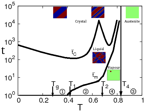
Figure 1: Temperature-Time-Transformation: Log-linear plots of mean martensitic conversion times ${\bar{t}}_{m}(T)$ and domain-wall orientation times ${\bar{t}}_{C}(T)$ versus quench temperatures $T$. Pictures are snapshots of domain-wall ’vapour’ ($\bar{t}_{m}>t$), ’liquid’ ($\bar{t}_{C}>t>\bar{t}_{m}$) and ’crystal’ ($t>\bar{t}_{C})$. Quench regions are indicated: Region 4 with $T_{4}>T>T_{2}$; Region 2 with $T_{2}>T>T_{1}$; and Region 1 with $T_{1}>T>T_{g}$.

Re-equilibration under a quench-and-hold protocolR16 , is described by the dynamic structure factor

$$\rho(\vec{k},t)\equiv|S(\vec{k},t)|^{2},~{}~{}~{}(2.3)$$

and its BZ average is the martensite fraction:

$$\sum_{\vec{k}}\rho(\vec{k},t)/N=\sum_{\vec{r}}S^{2}(\vec{r},t)/N=n_{m}(t).~{}~{}(2.4)$$

Fig 1 shows schematic curves from the dataR12 ; R16 , of the Temperature-Time-Transformation (TTT) evolution of the seeded system, quenched to a temperature $T$.The free-running system is monitored as it passes through domain wall phases of vapour, liquid and crystal. The martensitic conversion time $t_{m}(t)$ where $n_{m}(t_{m})=0.5$, is also the TTT phase boundary between vapour and liquid. There is also another time $t_{C}(T)$ for the orientation of domain walls, that will be considered elsewhere.

We will consider three temperatures in three distinct temperature Regions R12 . For $T_{4}>T=0.76>T_{2}$ in Region 4, the re-equilibration is dominated by the vapour-to-liquid or conversion delayR20 $t_{m}(T)$. For $T_{2}>T=0.55>T_{1}$ in Region 2, the total delay also has contributions from the liquid-to-crystal delay $t_{C}(T)$. Finally, for $T_{1}>T=0.4$ in Region 1, the conversion time is negligible, and the domain-wall orientation time $t_{C}(T)$ dominates. In Region 3, even though the quenched temperature is still below the Landau transition temperature $T_{0}=1>T>T_{4}=0.824$, the small, dilute martensitic seeds disappear into surrounding metastable austenite, and are not re-nucleated. Hence in Region 4 we study a $T=0.76$ sufficiently below $T_{4}$, for a reasonable number of the $N_{runs}=100$ to convert, in a reasonable time.

III Textural evolution in Fourier space

Fig 2a) shows that for a quench to $T=0.76$ the Hamiltonian energy of (2.1) is nearly flat, with $H(t)\simeq 0$, up to $t\sim t_{Sm}$. It starts to go negative at $t\sim t_{1}\sim 0.85~{}t_{m}$; and falls rapidly at $t=t_{m}$. The fall slows down at $t\sim t_{SC}$, and finally flattens at $t\sim t_{C}$. By contrast, for a quench to $T=0.4$ in Region 1, the energy drops almost immediately. Fig 2b) shows the austenite fraction $n_{0}(t)\equiv 1-n_{m}(t)$ behaves similarly, incubating at $n_{0}(t)=n_{0}(0)\simeq 1$ for $T=0.76$ before falling; while being expelled immediately, for $T=0.4$.

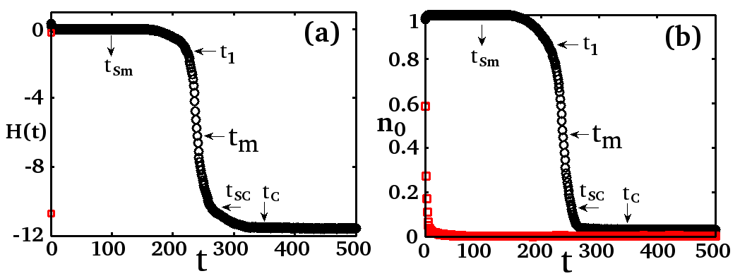
Figure 2: Energy and austenite fraction evolutions: For $T=0.76,0.4$ in quenched-temperature Regions 4 and 1 respectively, the falloff of a) the Hamiltonian energy, $H(t)/N$ vs $t$; and b) the austenite fraction $n_{0}(t)\equiv 1-n_{m}(t)$ vs $t$.

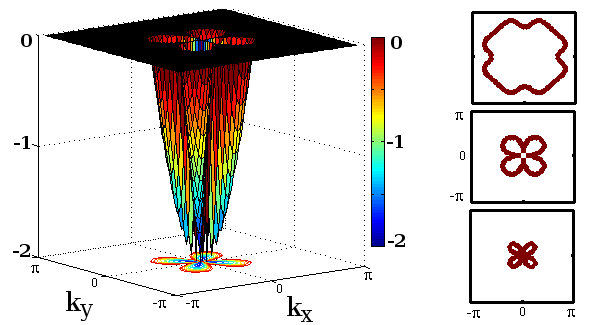
Figure 3: (Color online) Golf holes and funnels. Relief plot for $T=0.76$ of relevant martensitic spectrum $\epsilon(\vec{k})$ versus $\vec{k}$ in the Brillouin zone, with a zero-energy plane. Sidebar: Golf hole edges $\epsilon(\vec{k})=0$, for quench temperatures top to bottom, that are low $T=0.42$ (explosive conversions); medium $T=0.76<T_{4}$ (slow, rarer conversions); and high $T=0.91>T_{4}=0.824$ (no conversions, divergent entropy barriers).

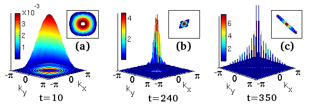
Figure 4: (Color online) Structure factors for domain-wall phases: Relief plots of $\ln[1+|S(\vec{k},t)|^{2}]$ versus $(k_{x},k_{y})$ in the Brilliouin Zone for a) vapour; b) liquid; c) crystal. Insets: Corresponding contour plots.

Since the evolving energy is first zero, and then negative, the relevant spectrum is thus a zero-energy plane through the $\epsilon(\vec{k})$ surface, plus the negative energies below it. Fig 3 shows that the resulting relief plot naturally depicts a flat surface containing a golf hole defined by $\epsilon(\vec{k})=0$, and a funnel $\epsilon(\vec{k})<0$ inside it. The sidebar shows the temperature-dependent, anisotropic golf hole edge, that is large (small) at low (high) temperatures.There is an outer (inner) squared-radius of $K^{2}={G_{\pm}}^{2}\simeq 2/R_{c}(T)\pm\delta$ with $\delta\equiv(A_{1}{\bar{V}}/2\xi_{0}^{2})>0$, where the average is $2/R_{c}\equiv-(g_{L}/\xi_{0}^{2})-\delta~{}>~{}0$.

Protein folding is understood through concepts such as golf holes and funnels in configuration space R2 ; R3 . Here, we find such concepts appearing naturally in martensitic re-equilibration, but in a more easily represented form in the label space $\vec{k}$ of strain modes, in which the Hamiltonian is diagonal. For protein folding, this would correspond to the label space of folding normal-modes, of the protein model Hamiltonian.

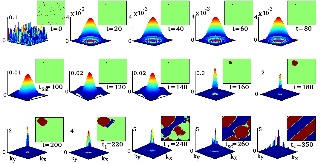
Figure 5: (Color online) Textural evolutions: Snapshots of Fourier-space strain structure factors as $\ln[1+|S(\vec{k},t)|^{2}]$ for successful conversions, after a quench to $T=0.76$. Insets show coordinate-space textures $\{S(\vec{r},t)\}$, with green (blue/red) denoting austenite (martensite variants). See the movie. The martensite fraction conversion time is $t_{m}(T)$. Other crossover times $t_{Sm},t_{1},t_{SC},t_{C}$ are defined in the text, and Fig 2.

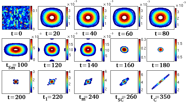
Figure 6: Contour plots of structure factor in Fourier space: Colour contour version of Fig 4 snapshots of $ln[1+|S({\vec{k}},t)|^{2}]$ for $T=0.76$. The three domain wall phases: vapour, liquid, crystal correspond to three contours: isotropic gaussian (e.g $t=80$), X-shaped (e.g $t=200$), single diagonal or fan-shaped (e.g $t=t_{C}\simeq 350$).

Fig 4 shows the Fourier-space structure factors $\{\rho(\vec{k},t)\equiv|S(\vec{k},t)|^{2}\}$ as relief plots, for domain-wall phases of ‘vapour’, ‘liquid’, and ‘crystal’. Fig 5 shows the MC evolutions that transform the phases into each other.

We first discuss the insets of Fig 5, that are the evolving coordinate space textures $\{S(\vec{r},t)\}$ as previously R12 , but now labelled by the characteristic times of Fig 2. See the movie in Supplementary Material. The insets show that the random seeds quickly form a vapour droplet of zero energy, that fluctuates in place up to a time $t=t_{Sm}\sim 100$: it is in an ‘incubating’ or ageing state R6 ; R8 ; R12 . The single-variant droplet then finds and enters an energy-lowering, autocatalytic-twinning channel R17 of alternating opposite variants, around a time $t=t_{1}\sim 220$. At a time $t=t_{m}\sim 240$, a domain-wall liquid forms, with walls of wandering orientation. After a symmetry-breaking choice of a diagonal at $t=t_{SC}\sim 260$, a domain wall crystal of oriented twins forms, beyond $t=t_{C}\sim 350$.

The main Fig 5 shows the same evolving textures, but now in Fourier space. See also Fig 4 and Fig 6. For $t<t_{Sm}$, the ageing state $\rho(\vec{k},t)$ for the incubating vapour droplet persists unchanged as a broad, isotropic gaussian, poised over the butterfly-shaped golf hole of Fig 3. One might expect the gaussian to promptly distort along diagonals, to fit into the correspondingly anisotropic golf hole, and narrow, to enter the negative energy funnel. Surprisingly, it does not do this. For $t>t_{Sm}\sim 100$, it waits in an incubation stage, to develop wings along $k_{x},k_{y}$ axes. See also the contour plots of Fig 6, at these times. Then for $t<t_{1}$ the peak narrows and then rises sharply, and for $t_{m}>t>t_{1}$, enters the golf hole, where it adopts the bi-diagonal symmetry of the funnel. After a symmetry-breaking at $t\sim t_{SC}$, the structure factor at $t>t_{C}$ is along a single diagonal. Thus the Fourier space distribution develops mis-oriented wings along the axes, before it forms wings along the Compatibility-favoured diagonals. In coordinate space, the austenitic $S=0$ spins at the droplet surface must flip collectively to produce $S=\pm 1$ surface spin regions of the right symmetry: much like a kinetic constraint R7 , but here self-generated. The improbability of finding this collective-spin distortion constitutes the entropy barrier.

Fig 6 shows the contour plots in the BZ corresponding to the relief plots of the main Fig 5. The $\rho(\vec{k},t)$ value of a point on such contours represents the Fourier intensity or ‘occupancy’, at a given $\vec{k}$. It would also be interesting to monitor the evolving occupancy at a given energy. We define the energy occupancy distribution $\rho(\epsilon,t)$, similarly to that of a protein-folding simulation R4 ,

$$\rho(\epsilon,t)=\frac{\sum_{\vec{k}}\delta_{\epsilon,\epsilon(\vec{k})}\rho(\vec{k},t)}{\sum_{\vec{k}}\rho(\vec{k},t)}.~{}~{}(3.1)$$

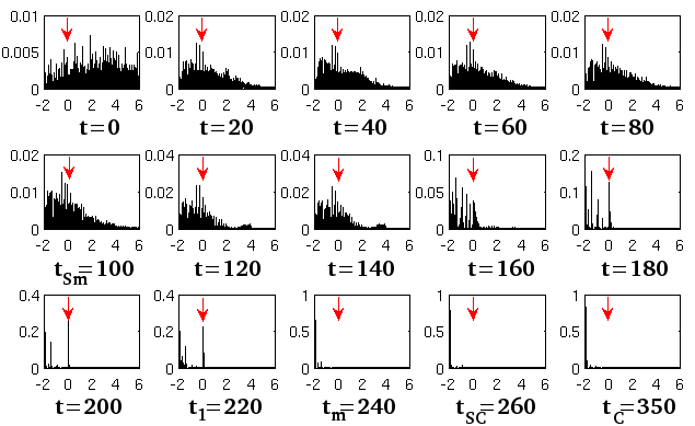
Figure 7: Time evolution of single-run energy occupancy distributions : Plots of $\rho(\epsilon,t)$ versus $\epsilon$ for quench to $T=0.76$ for a single run, at various times. Arrow marks the golf hole, of energy $\epsilon=0$. The funnel region is $0>\epsilon>g_{L}=-|g_{L}|$. A small peak at large energies appears on the formation of the entropically critical droplet for $t>t_{Sm}\simeq 100$; and an occupancy spike from an entropy barrier persists at the golf hole energy right up to $t=t_{m}\simeq 240$.

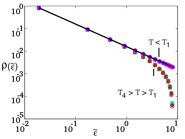
Figure 8: Final energy occupancy distributions: Log-log plot of $\rho({\tilde{\epsilon}},t)$ versus $\tilde{\epsilon}\equiv\epsilon-g_{L}$ showing final $1/\tilde{\epsilon}$ behaviour, regardless of quench temperature, and of different energy scales $E_{0}=3,4,5,6$. Solid line has a slope $-1.0$; and an estimated upper energy cutoff R21 is $\simeq 9.1$, consistent with simulations.

Fig 7 shows the evolving histogram of the single-run $\rho(\epsilon,t)$ versus energy $\epsilon$. The arrow marks the energy $\epsilon=0$ of the golf hole edge. The negative energies $0>\epsilon>g_{L}$ are the funnel region. The distribution remains fixed, up to $t=t_{Sm}=100$, and then a small positive energy peak appears, corresponding to the wings along the axes of Fig 6. (It appears at different onset times in different runs, so a time average would wash it out.) The weight of the distribution moves more into the negative energy region, and by around $t=t_{m}=240$, it is almost entirely in the funnel. Note the long-lived, occupancy spike at the energy of the golf hole edge and its environs R3 . This disappears at $t_{m}$, on crossing of the entropy barrier.

As shown in Fig 8 the final distribution, for all quenches, is an inverse-energy falloff in the excitation energy above the bulk Landau term, $\tilde{\epsilon}\equiv\epsilon-g_{L}>0$:

$$\rho({\tilde{\epsilon}},t;T)\rightarrow 1/{\tilde{\epsilon}}.~{}~{}~{}(3.2)$$

For a continuous-variable displacement of a harmonic oscillator, averaging with a Boltzmann factor would yield the same inverse-energy behaviour. The form is also independent of Hamiltonian energy scales $E_{0}$ and anisotropic stiffness constants $A_{1}$. Since the domain walls are sparse, and discrete, the energies are also discrete. The energy has an upper cut off, that is estimated R21 as $\log_{10}{(\tilde{\epsilon})}\lesssim 9.1$, consistent with the simulation results.

Notice that although the distribution $\rho(\vec{k},t)$ or $\rho(\epsilon,t)$ of Fig 5 or Fig 7 has much of its weight poised above the funnel states inside the golf hole, these domain-wall modes labelled by $\vec{k}$ or $\epsilon$, do not immediately collapse into available negative energy states. Re-equilibration does not follow a strategy of ’every mode for itself’. Rather there is an ‘all modes together’ strategy: the modes first partially equilibrate so there is no net inter-mode energy exchange, setting up some nonequilibrium mode-distribution; followed by a slower emergence, as entropy barriers are crossed, of an equilibrium mode-distribution at the bath temperature.

IV Conversion delays: Entropy barrier crossing

We need to understand how conversion delays from entropy barriers, can be so drastically different, at nearby temperatures. At low temperatures of Region 1 of $T<T_{1}=0.42$, seeds in austenite convert explosively to martensite variants, for every run. At very high temperatures of Region 3 of $T_{0}=1>T>T_{4}=0.82$ there is a complete ‘blocking’ of conversion to energy-lowering martensite, with the zero-energy seeds dissolving for every run, into zero-energy austenite. And for Region 4 of $T_{4}>T>T_{2}=0.68$ there is a rise in both the conversion time and the fraction of blocked runs on approaching $T_{4}$, so the mean time diverges like a Vogel-Fulcher lawR1 ; R12 ${\bar{t}}_{m}(T)\sim e^{|\Delta S|}\sim e^{1/(T_{4}-T)}$.

An understanding of entropy barriers $|\Delta S|$ that are either zero, sharply rising, or infinite, comes from quenches to Region 4, with a Fourier distribution $\rho(\vec{k},t)$ that starts as an isotropic gaussian and ends as an inverted fan along one diagonal, as in Figs 4, 5. We parametrize the distribution through a weight $\eta$ of the emerging anisotropy.

The distribution is separated, outside the golf hole ($t<t_{1}$), and inside the funnel ($t>t_{1}$), as

$$\rho(\vec{k},t)=\rho_{g}(\vec{k},\eta)\theta(t_{1}-t)+\rho_{f}(\vec{k},\eta)\theta(t-t_{1}).~{}~{}(4.1)$$

We will focus on the constrained search pathways outside the golf hole for $t<t_{1}$, through the parametrization

$$\rho_{g}=N\{n_{m}(0)(1+b_{g}\eta(t))+\eta(t)\cos 4\theta\}C_{g}e^{-{{\vec{K}}^{2}}/2\sigma^{2}},~{}~{}(4.2)$$

where $C_{g}$ normalises the gaussian to unity, and $b_{g}\equiv{n_{m}(0)}^{-1}-{n_{m}(t_{1})}^{-1}$. The evolution parameter $\eta(t)$ then carries the fourfold anisotropy of the kernel of (2.1c), as $\rho_{g}\sim\eta(t)(1+\cos 4\theta)$. Here the normalisation (2.4) yields $\eta(t)=[(n_{m}(t)/n_{m}(0))-1]/b_{g}>0$. The distribution is isotropic with $\eta(t)=0$, during the $n_{m}(t)=n_{m}(0)$ incubation for $t_{Sm}>t$. Whereas for $t_{1}>t>t_{Sm}$ a nonzero $\eta>0$ induces an angular modulation, that increases the distribution at $\theta=0,\pi/2..$, i.e. along the $k_{x},k_{y}$ axes.

Writing the $\vec{k}\neq 0$ Hamiltonian energy of (2.1) as averages $<...>$ over the distribution (4.2), so

$$H/Nn_{m}=\xi_{0}^{2}<{\vec{K}}^{2}>+g_{L}+(A_{1}/2)<{\tilde{V}}(k)>,~{}~{}(4.3a)$$

we obtain on the zero-energy plane outside the golf hole, a constraint linking the Ginzburg, Landau and St Venant contributions,

$$H/Nn_{m}\xi_{0}^{2}=\{2\sigma^{2}-2/R_{c}\}+\{\eta(t)/n_{m}(t)\}\delta/2=0.~{}~{}~{}(4.3b)$$

In the $\eta=0$ ageing state the average golf hole radius determines the gaussian width or inverse droplet size as $2\sigma^{2}=2/R_{c}$. From the constraint of (4.3b), any decrease in width must be compensated by an increase in mis-orientation energy $\sim\delta\sim A_{1}{\bar{V}}$ of the last term: the $\eta>0$ wings must indeed, first emerge along the axes, before the diagonals. This explains the observed $\rho(\vec{k},t)$ distortions, of Figs 5,6 for $t_{1}>t>t_{Sm}$. At $t=t_{1}$, when $\eta(t_{1})=n_{m}(t_{1})$, the width from (4.3b) narrows to $2\sigma^{2}=(2/R_{c})-\delta/2$; and then to the inner radius. If $\eta$ is (unphysically) taken to be negative, favouring diagonal wings right away, then the constraint of (4.3b) makes the width larger, going in the wrong direction.

The delays $t_{m}\sim e^{|\Delta S|}$ are understood through the temperature-dependent golf holes in the sidebar of Fig 3. For $T$ below $T_{1}$, the golf hole in the BZ is large, and the flat distribution from seeds directly forms a liquid distribution of Fig 4, entering the funnel immediately for every run. The conversion time is negligible, and its entropy barrier is zero, $|\Delta S|\simeq 0$. For $T$ approaching $T_{4}$ the golf hole shrinks, and hence the search times rise; the entropy barrier diverges as $|\Delta S|\sim 1/(T_{4}-T)$, and the fraction of runs converting to martensite falls, yielding Vogel-Fulcher behaviour. For $T>T_{4}$ the golf hole inner radius $G_{-}^{2}$ closes, and the resulting 4-petalled golf hole topology presents the isotropic gaussian with an infinite entropy barrier. Thus even though the martensite Landau energy is lower than the austenite energy for $T_{0}>T>T_{4}$, it becomes ergodically inaccessible R8 to the small and dilute initial seeds.

For nucleation by activation over energy barriers, a divergent droplet timescale is associated with a divergent size in coordinate space. By contrast, for non-activated entropy barrier crossing, a divergent search timescale for droplet pathways is associated with a shrinking bottleneck in Fourier space.

Under MC dynamics for a given run $n$, the total Hamiltonian energy $H(t)$ of a texture $\{S(\vec{r},t)\}$ goes to $H(t+1)$ at the next MC sweep. The probability for a given energy change $\Delta E$ to occur at a time $t$, from Hamiltonian increments $\Delta H(t,n)=H(t+1)-H(t)$, is obtained through an average over all runs $n=1,2...N_{runs}$:

$$P(\Delta E,t)\equiv\frac{1}{N_{runs}}\sum_{n=1}^{N_{runs}}\delta_{\Delta H(t,n),\Delta E}.~{}~{}(4.4a)$$

At early times, the probability is peaked at negative values $\Delta E=-|\Delta E|<0$, with an asymmetric shoulder on the negative side R7 ; and at long times, this becomes an equilibrium distribution, symmetric around zero (not shown). To determine if there is a dominant energy change during the evolution, regardless of when it occurs, we average the energy release probability over the entire holding time, $P(\Delta E)\equiv\sum_{t}P(\Delta E,t)/t_{h}$.

Fig 9 shows $P(\Delta E)$ for various temperatures and energy reductions. There are a few large magnitudes of energy release, but mostly, $P(\Delta E)$ falls as a powerlaw in the magnitudes $\sim 1/|\Delta E|^{\gamma}$, with a common exponent $\gamma\simeq 2$. This suggests that the domain-wall adjustments have no characteristic energy scale, and are like small earthquakes, of all scales. Acoustic emissions occur in martensites, from twin boundaries inducing energy changes, and power law distributions have been seen R22 with exponent close to $2.3$.

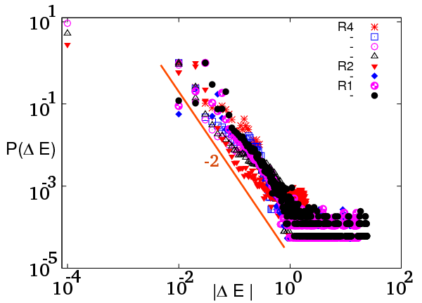
Figure 9: Probability distribution of energy releases: Log-log probability of energy releases at any time, $P(\Delta E)$, versus magnitude of releases $|\Delta E|$.

The Monte Carlo acceptance fractionR6 $A_{acc}(t)$, is the fraction of $N$ sites where the MC move is accepted during a given sweep at $t$. Ageing non-interacting oscillators, have small and monotonically decreasing R6 $A_{acc}\sim 1/t\ln t$, from an inefficient, memory-less search of all oscillators, for an ever-decreasing un-relaxed population.

Figure 10 shows for this model, the very different acceptance fractions $A_{acc}(t)$ versus time $t$ for the three Regions. At $T=0.76$ in Region 4, $A_{acc}(t)$ is nearly zero during incubation. The acceptance spikes at conversion times $t=t_{m}$ during conversion from domain-wall vapour to liquid, and falls again to zero beyond $t=t_{C}$, in the crystal phase. The spike occurs at the same time as the sharp rise of the martensite fraction through $n_{m}(t_{m})=0.5$, giving a physical justification to this earlier definition of $t_{m}$.

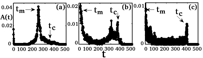
Figure 10: Monte Carlo Acceptances : Plot of $A_{acc}(t)$ versus $t$ for the three temperature-quench Regions 4, 2, 1. a) $T=0.76$ in Region 4; b) $T=0.55$ in Region 2; c) $T=0.4$ in Region 1.

For $T=0.55$ in Region 2, $A_{acc}(t)$ is high initially, accepting most of the flips; decreases when the domain wall liquid phase is reached; peaks again near $t=t_{C}$ on domain wall orientations; and finally falls to zero acceptances in the crystal phase. There can be a second peak just before $t=t_{C}$, where austenite droplets are generated to bind to the domain walls R12 . For $T=0.4$ in Region 1, the acceptance in the liquid phase is spiky, during domain wall motion in the liquid phase. Then there is a peak in $A_{acc}(t)$, as a large number of austenite droplets or hotspots are generated to catalyse domain-wall symmetry-breaking orientations R12 , finally falling to zero as before, in the crystal.

The ageing state has MC acceptance fractions that are nearly zero, and acceptance spiking at $t_{m}$ or $t_{C}$ is thus a diagnostic at all temperatures for the crossing of an entropy barrier.

V Domain-wall thermodynamics and effective temperatures

We approximate the MC Hamiltonian $H(t)$ by that of independent spins at $T$, in a time-dependent local mean-field R12 $\sigma(\vec{r},t)$, where the non uniformity comes from the domain walls. This implicitly assumes (consistent with simulations) that there is a separation of time scales, with individual spins flipping rapidly in response to quenches of the temperature, with domain wall configurations evolving more slowly. The Appendix obtains, within a ‘time-dependent local mean-field’ approximation, expressions for the free energy $F\simeq F_{LMF}(t)$, internal energy $U(t)$, and entropy $S_{entr}(t)=-F_{LMF}(t)+TS(t)$, in terms of the $\{S(\vec{r},t)\}$ configurations at a given MC sweep labelled by $t$.

We regard the domain-walls under stress as internal work sources, that run freely after a quench. The overall change in the internal energy $dU(t)$, by a First Law type relation, is a sum of contributions from the work done by domain walls ${d\mkern-5.0mu\mathchar 22\relax}W(t)$, and the heat release $d\mkern-5.0mu\mathchar 22\relax Q(t)$:

$$dU(t)=d\mkern-5.0mu\mathchar 22\relax W(t)+d\mkern-5.0mu\mathchar 22\relax Q(t).~{}~{}(6.1)$$

We need relations between the textural thermodynamics and increments in the heat and the work, at constant $T$. The heat release by spins, that are at the bath temperature, is taken as $d\mkern-5.0mu\mathchar 22\relax Q(t)=TdS_{entr}(t)$. For equilibrium, the Helmholtz free energy change between thermodynamic states, is the available work at constant temperature R23 . We assume the free-running work increment at constant temperature saturates a similar availability, set by the evolving free energy change: $d\mkern-5.0mu\mathchar 22\relax W(t)=dF_{LMF}(t)$. At long times after entropy barriers are crossed, thermodynamic equilibration $dF=0$ is accompanied by mechanical equilibration $d\mkern-5.0mu\mathchar 22\relax W=0$.

The evolving work rate is ${\dot{W}}(t)$, and the heat emission rate is ${\dot{Q}}(t)$, where ‘rates’ are $X(t+1)-X(t)\equiv{\dot{X}}(t)$. Fig 11 shows the probability distributions $P(\dot{W}),P(\dot{Q})$ over MC runs, for the rates of internal work done or heat emitted. They can peak at negative values, but finally both equilibrate to peaks centred at zero. Fig 12 shows that the mean rates of work done and heat emitted are suppressed in the ageing state by entropy barriers, but show large and sudden releases, as the entropy barriers are crossed. On equilibration, all mean rates tend to zero.

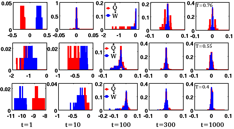
Figure 11: Evolution of distributions for rate of heat emission and internal work : Plot of evolving $P(\dot{Q},t)$ versus $\dot{Q}$ and $P(\dot{W},t)$ versus $\dot{W}$ for quenches into the three Regions 4, 2, 1. Top row: $T=0.76$ in Region 4. Middle row: $T=0.55$ in Region 2. Bottom row: $T=0.4$ in Region 1. For all $T$, the final distributions are peaked symmetrically around zero.

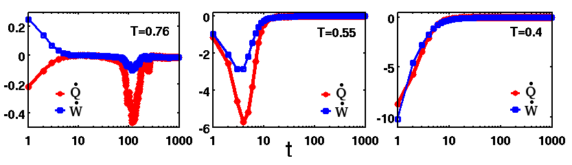
Figure 12: Evolution of averaged rates of heat emission and internal work: Log-linear plots shows the mean rates $<\dot{W}>$ and $<\dot{Q}>$ versus the time $t$. For $T=0.76$, the rates are zero in the ageing state, have large releases near ${\bar{t}}_{m}(T)$, and finally vanish on equilibration. For $T=0.55,0.4$ the curves are similar, but moved to the left, as conversion delays $t_{m}$, vanish. For all $T$, the final mean rates are zero.

The energy of trapped stresses can only escape as heat released to the bath, since the boundary conditions are periodic, and not piston-like. One would like to relate a stress-induced heat release to re-equilibration of some effective temperature, that has otherwise been defined in terms of the Fluctuation-Dissipation relation R24 .

In the equilibrium case, and for some externally imposed work protocol R25 , one can distinguishR26 between heat changes (that are occupancy changes of given energy levels), and work changes (that are energy levels changes at fixed-occupancy). For temperature quenches, however, there is no such external sequential control, and both work and heat changes occur together. The relative proportion of spontaneous heat and work in (6.1) can be tracked, by defining a $T_{eff}(t)$,through

$$d\mkern-5.0mu\mathchar 22\relax W(t)\equiv[1-\frac{T}{T_{eff}}]dU(t);~{}~{}~{}d\mkern-5.0mu\mathchar 22\relax Q(t)\equiv\frac{T}{T_{eff}}dU(t).~{}~{}~{}(6.2)$$

With the previous increment relations this is manifestly equivalent to a ’microcanonical’ definition, $T/T_{eff}(t)=TdS_{entr}(t)/dU(t)$, as invoked in protein folding models R4 .

The incremental work can also be related to changes in the local mean-field,

$$d\mkern-5.0mu\mathchar 22\relax W(t)\simeq-\sum_{r}p(\vec{r},t)\delta\sigma(r,t)~{}~{}(6.3)$$

where the local stress is $p(\vec{r},t)=\partial F_{LMF}(t)/\partial\sigma(r,t)$. For static textures at equilibrium $\sigma(r,t)={\bar{\sigma}}(\vec{r})$ satisfying the mean-field self-consistency condition R27 , the local stresses vanish in the domain-wall crystal phase R12 , as seen in the Appendix. From $d\mkern-5.0mu\mathchar 22\relax W\sim(1-T/T_{eff})$ of (6.2), this vanishing of trapped stresses is consistent with $T_{eff}(t)\rightarrow T$. A detailed study of this final equilibration would involve the second entropy barrier at $t_{C}$, and so the trapped-stress related effective temperature will be pursued elsewhere.

VI Summary

We develop a detailed understanding of the re-equilibration process of domain walls, in a martensite-related three-state model with powerlaw anisotropic interactions. There is a natural appearance of concepts borrowed from protein folding, of golf holes and funnels; and from oscillator relaxation models, of Monte Carlo acceptance fractions. As found earlier, domain-wall phases after a quench, evolve from a domain-wall ’vapour’ to a ’liquid’, and thence to a ‘crystal’ of oriented walls. There is a temperature regime where the martensite conversion delay $t_{m}$ dominates the total delay. The evolution from a vapour-phase zero-energy droplet in zero-energy austenite to a negative-energy liquid of martensite domain walls, is best understood in Fourier space. The droplet has an isotropic gaussian structure factor, peaked at the Brillouin zone centre, over a butterfly-shaped, small golf hole with a negative energy funnel inside. The incubation delays come from a search for anisotropies at zero energy to roll into the golf hole. At low temperatures, the golf hole is large, and conversion from seeds occurs almost immediately. At temperatures above transition, there is golf hole topology change, preventing the roll-in, and suppressing the conversion of austenite.

In the ageing state, the MC acceptance fractions are negligible; both work and heat rates are zero; and trapped local stresses are held in place by entropy barriers. On crossing entropy barriers at the death of ageing, there are spikes in the MC acceptance, and sudden releases of the trapped stress and heat. On the resultant thermal and mechanical re-equilibration, acceptance fractions for spin-flips again vanish; work and heat rates are zero; and the oriented domain walls are stress-free, with a related effective temperature going to the bath temperature. The scenario may have relevance to other models of athermal re-equilibration after a quench, such as glassy and granular models.

It is a pleasure to thank Shamik Gupta, Uwe Klemradt, Stefano Ruffo, VSS Sastry and Sandro Scandolo for useful conversations. NS thanks the University Grants Commission, India for a Dr. D.S. Kothari postdoctoral fellowship.

Appendix : Time-dependent local mean-field approximation :

The uniform, static mean-field approximation is familiar for ferromagnets, and antiferromagnets (where it is a staggered magnetisation). However a static, local mean-field can faithfully reproduce the domain-wall textures from simulationsR27 . This can be generalized R12 to an MC time-dependent local mean-field approach, to describe the evolving domain walls.

The model Hamiltonian of (2.1) has the bath temperature $T$ entering $H(T)$ through the martensitic strain magnitudes ${\bar{\varepsilon}}(T)$. With the partition function as $Z=\sum_{\{S\}}e^{-H(T)/T}$, and the canonical free energy as $F=-T\ln Z$, the entropy is $S_{entr}=-\partial F/\partial T$, the internal energy defined by $U\equiv F+TS_{entr}$, is then not just the averaged hamiltonian, but is

$$U=<H>-<T\partial H/\partial T>.~{}~{}~{}(A1)$$

With strain-pseudospin patterns $\{S(\vec{r},t)\}$ evolving under Monte Carlo dynamics, the weight factor $e^{-H/T}$is truncated within R12 a ‘time-dependent local mean-field approximation’ that we restate here for completeness. It is defined by the substitution into the coordinate space Hamiltonian as

$$S(\vec{r})S(\vec{r}^{\prime})\rightarrow S(\vec{r})\sigma({\vec{r}}^{\prime},t)+\sigma(\vec{r},t)S(\vec{r})-\sigma(\vec{r},t)\sigma({\vec{r}}^{\prime},t).~{}(A2a)$$

Here, the mean field spin $\sigma$ is defined as a run-average of a local spin variable at a site $\vec{r}$, and an MC time $t$:

$$\sigma(\vec{r},t)\equiv<S(\vec{r},t)>.~{}~{}(A2b)$$

The local mean-field weight is then $e^{-H/T}\rightarrow e^{-H_{LMF}/T}$ where

$$H_{LMF}/T=\sum_{\vec{r}}q(\vec{r},t)S(\vec{r},t)-\frac{1}{2}\sum q(\vec{r},t)\sigma(\vec{r},t)~{}~{}~{}(A2c)$$

depends on individual spins in a mean-field, and

$$q(\vec{r},t)\equiv\sum_{\vec{r}^{\prime}}q_{0}(\vec{r}-\vec{r}^{\prime})\sigma(\vec{r}^{\prime},t),~{}~{}(A2d)$$

where

$$q_{0}(\vec{r}-\vec{r}^{\prime})\equiv D_{0}[\{g_{L}(\tau)+\xi_{0}^{2}{\Delta_{\vec{r}}}^{2}\}\delta_{\vec{r},\vec{r}^{\prime}}+\frac{A_{1}}{2}V(\vec{r}-\vec{r}^{\prime})].~{}(A2d)$$

As mentioned in the text, the individual spins are assumed to respond instantaneously to the quenched temperature of the heat bath and to the influence of domain walls, that themselves evolve much more slowly, under MC dynamics.

The corresponding substitution in the Fourier space Hamiltonian of (2.1) is

$$|S(\vec{k})|^{2}\rightarrow S(\vec{k})\sigma(\vec{k},t)^{*}+\sigma(\vec{k},t)S(\vec{k},t)^{*}-|\sigma(\vec{k},t)|^{2}.~{}~{}(A3a)$$

Here

$$H_{LMF}/T=\sum_{\vec{k}}q(\vec{k},t)^{*}S(\vec{k},t)-\frac{1}{2}q_{0}(\vec{k},t)|\sigma(\vec{k},t)|^{2},~{}~{}~{}(A3b)$$

where

$$q(\vec{k},t)\equiv q_{0}(\vec{k})\sigma(\vec{k},t),~{}~{}(A3c)$$

and

$$q_{0}(\vec{k})\equiv D_{0}[\{g_{L}(\tau)+\xi_{0}^{2}{\vec{K}}^{2}\}+\frac{A_{1}}{2}{\tilde{V}}({\vec{k}})(1-\delta_{\vec{k},0})]~{}~{}(A3d)$$

with $D_{0}(T)\equiv K_{0}/T=2\bar{\varepsilon}^{2}(\tau)E_{0}/T$.

The thermodynamic functions are all taken as zero in $S=0$ uniform austenite, and the approximate $LMF$ free energy is

$$F_{LMF}=-T\{\sum_{\vec{r}}\ln\frac{1}{3}[1+2\cosh q(\vec{r})]-\frac{1}{2}\sum_{\vec{k}}q_{0}|\sigma(\vec{k})|^{2}\},~{}(A4)$$

The internal stress $p(\vec{r},t)=\partial F_{LMF}/\partial\sigma(\vec{r},t)$ is

$$p(\vec{r},t)=-\sum_{{\vec{r}}^{\prime}}q_{0}(\vec{r}-\vec{r}^{\prime})[\frac{2\sinh q(\vec{r}^{\prime},t)}{1+2\cosh q(\vec{r}^{\prime},t)}+\sigma(\vec{r}^{\prime},t)]~{}~{}(A5)$$

and vanishes at the self-consistent, static equilibrium textures R27 $\sigma(\vec{r},t)={\bar{\sigma}}(\vec{r})$, when the square bracket is zero.

From (A1) and the Hamiltonian (2.1), the internal energy is

$$U=[1-\frac{T}{{\bar{\varepsilon}}^{2}}\frac{d{\bar{\varepsilon}}^{2}}{dT}]<H>-E_{0}{\bar{\varepsilon}}^{2}T\frac{dg_{L}}{dT}\sum_{\vec{k}}<|\sigma(\vec{k})|^{2}>,~{}~{}(A6)$$

where the averages are with the $LMF$ weight. The entropy is taken as the difference of (A4), (A6)

$$TS_{entr}=-F_{LMF}+U.~{}~{}(A7)$$

With $Td/dT=[\tau(T)-\tau(0)]d/d\tau$ and the definitions of the text, $Td{\bar{\varepsilon}^{2}}/dT=-[\tau(T)-\tau(0)]/(4\sqrt{1-3\tau/4})$; and $Tdg_{L}/dT=[\tau(T)-\tau(0)][1-2{(\bar{\varepsilon}}^{2}-1)/(4\sqrt{1-3\tau/4})].$

Of course, these expressions are in terms of the time-dependent local mean-field $\sigma(\vec{r},t)$. We sidestep the evaluation through (A2b) of $\sigma(\vec{r},t)$ at each time $t$, by invoking the spirit of mean-field approximations, namely that
‘the function of an average is an average of the function’, and taking

$$F_{LMF}(\{\sigma(\vec{r},t)\})\simeq<F_{LMF}(\{S(\vec{r},t)\})>;~{}~{}~{}(A8a)$$

$$U(\{\sigma(\vec{r},t)\})\simeq<U(\{S(\vec{r},t)\})>;~{}~{}~{}(A8b)$$

where the averages are now taken over each distinct MC runs.

Thus the (time-dependent) $LMF$ expressions of (A4), (A6), (A7) yield expressions for the domain-wall thermodynamics of an evolving texture $\{S(\vec{r},t)\}$ over a each distinct re-equilibration run, that can then be averaged over many runs. This approach has been used for Figs 11,12.

References

- (1) K. Binder and W. Kob, Glassy Materials and Disordered Solids : An Introduction to Their Statistical Mechanics, World Scientific, Singapore (2005).
- (2) P.G. Wolynes, J. Onuchic and D. Thirumalai, Science 267, 1619 (1995); P.G. Wolynes, Proc. of the Am. Phil. Society 145, 4 (2001); M. Cieplak and I. Sulkowska, J. Chem. Phy. 123, 194908 (2005).
- (3) D. J. Bicout and A. Szabo, Protein Science 9, 452 (2000).
- (4) N. Nakagawa and M. Peyrard, PNAS 103, 5279 (2006); N. Nakagawa, Phys. Rev. Lett. 98, 128104 (2007).
- (5) F. Ritort, Phys. Rev. Lett. 75, 1190 (1995); S. Franz and F. Ritort, Europhys. Lett. 31, 507 (1995).
- (6) L. L. Bonilla, F.G. Padilla and F. Ritort, Physica A 250, 315 (1998); A. Garriga and F. Ritort, Phys. Rev. E 72, 031505 (2005).
- (7) F. Ritort and P. Sollich, Adv. Phys. 52, 219 (2003).
- (8) A. Campa, T. Dauxois and S. Ruffo, Phys. Rep. 480, 57 (2009); H. Shintani and H. Tanaka, Nature Physics 2, 200 (2006).
- (9) Physical properties of martensite and bainite: Proceedings of the joint conference, the British Iron and Steel Research Association and the Iron and Steel Institute, Special report 93, London (1965); A. R. Entwhistle, Metall. Trans. 2, 2395 (1971); M. Rao and S. Sengupta, Current Science (Bangalore) 77, 382 (1999); V. Hardy, A. Maignan, S. Hebert, C. Yaicle, C. Martin, M. Hervieu, M.R. Lees, G. Rowlands, D. McK. Paul and B. Raveau, Phys. Rev. B 68, R220402 (2003); Y. Wang, X. Ren, K. Otsuka, Phys. Rev,. Lett. 97, 225703 (2006).
- (10) T. Kakeshita, K. Kuroiwa, K. Shimizu, T. Ikeda, A. Yamagishi, and M. Date, Materials Transactions, JIM, 34, 423 (1993); T. Kakeshita, T. Fukuda and T. Saburi, Scripta Mat. 34, 1 (1996); U. Klemradt, M.Aspelmeyer, H. Abe, L.T. Wood, S.C. Moss and E. Dimasi, J.Peisl, Mat. Res. Soc. Symp. Proc. 580, 293 (2000); L. Mueller , U. Klemradt, T.R. Finlayson, Mat. Sci. and Eng. A 438, 122 (2006); L. Mueller, M. Waldorf, C. Gutt, G. Gruebel, A. Madsen, T.R. Finlayson, and U. Klemradt, Phys. Rev. Lett. 107, 105701 (2011).
- (11) M. Baus and R. Lovett, Phys. Rev. A 44, 1211 (1991); S. Kartha, J. A. Krumhansl, J. P. Sethna, and L. K. Wickham, Phys. Rev. B 52, 803 (1995); S.R. Shenoy, T. Lookman, A. Saxena and A.R. Bishop, Phys. Rev. B 60, R12537 (1999); K.O. Rasmussen, T. Lookman, A. Saxena, A.R. Bishop, R.C. Albers and S.R. Shenoy, Phys. Rev. Lett. 87 (2001).
- (12) N. Shankaraiah, K.P.N. Murthy, T. Lookman and S.R. Shenoy, Europhys. Lett. 92, 36002 (2010); Phys. Rev. B 84, 064119 (2011); J. of Alloys and Compounds 577, S66 (2013).
- (13) P.A. Lindgard and O.G. Mouritsen, Phys. Rev. Lett. 57, 2458 (1986); E. Vives, J. Goicoechea, J. Ortin and A. Planes, Phys, Rev. E 52, R5 (1995); J.F. Blackburn and E.K.H. Salje, Phy. Chem. Miner. 26, 275 (1999); D. Sherrington, J. Phys.: Condens. Matter. 20. 304213 (2008).
- (14) S. R. Shenoy, T. Lookman and A, Saxena, Phys. Rev. B 82, 144103 (2010).
- (15) M. Blume, Phys. Rev. 141,517 (1966); H.W. Capel, Physica 32 , 966 (1966).
- (16) Instead of an isothermal martensite regime with activated conversion timesR12 , we work in an athermal regime where non-activated conversion times are insensitive to energy scales . At , the austenite background, seeded with variants, at of randomly located sites, is quenched to , that is held fixed for MC sweeps. Typical scaled parameters are R12 . Here; the holding time is ; and random-seed averages are over runs. For successful runs converting at a time , the rate is , and the inverse average rate defines a mean conversion time . (For runs where seeds vanish into austenite, and never return within , we set .) Close to , when conversions become rarer, we find R12 a Vogel-Fulcher behaviour , and a log-normal distribution for , insensitive to and to .
- (17) The autocatalytic, dynamic twinning channel for such field theories was found earlier in a 1D continuous-strain, underdamped dynamics, G.S. Bales and R. J. Gooding, Phys. Rev. Lett. 67, 3412 (1991); and in a 2D generalization, T. Lookman, S.R. Shenoy, K.O. Rasmussen, A. Saxena and A. R. Bishop, Phys. Rev. B 67, 024114 (2003). Similar behaviour was seen for purely relaxational dynamics without second-order time derivatives R11 . Here we use ‘autocatalytic twinning’ in this looser sense, of a generation of opposite-sign strain variants under any dynamics, including discrete-time MC dynamics (where increments can be regarded as formally including higher derivatives).
- (18) The Fourier amplitude is not just an independent oscillator displacement labelled by , since its (inverse) Fourier transform is constrained to be an integer .
- (19) A. Planes, F-J. Perez-Reche, E. Vives and L. Manosa, Scripta Mat. 50,181 (2004).The triple-well Landau variational function has Landau barriers to the conversion of metastable austenite for , implying one only has to wait long enough, in this range. However, in reviewing scenarios, KlemradtR10 noted that Otsuka found no conversion well below the Landau transition, even after a wait of 21 days. We have reconciled the three scenarios R12 , finding a divergence of delay times, well before the Landau transition .
- (20) The conversion delays are not due to discrete-lattice pinning effects, since if so, the delays would be longer at lower (as the Boltzmann probabilities for de-pinning would be smaller). But in our case, it is the other way round, and ‘cooler is faster’. The conversion delays are also not due to the trivial geometric requirement that domain walls must advance at unit steps along the square-lattice axes, (to form larger-scale serrated steps along the diagonal). Any such temperature-independent micro delays will also occur at low temperatures, and are seen to be at most a few MC time increments. The movie in Supplementary Material shows that the dynamic vapour phase droplet is like an ‘amoeba’, extending and withdrawing unit cell arms along the axes, and not simply advancing uniformly. In this incubation regime, the droplet is searching for the right correlated flips at its surface, that in Fourier space of Figs 5, 6 appear as wings along the axes. As explained in the text , this is a pathway for the distribution to rise in height and narrow in width, to enter the funnel, while still satisfying the zero-energy constraint of the golf hole and its environs.
- (21) The cutoff energy is the maximum value of . Estimating the two terms for diagonal or axis directions of , the upper bound on is . For , , estimated cutoff is , consistent with simulations.
- (22) F.J. Perez-Reche, E. Vives, L. Manosa and A. Planes, Phys. Rev. Lett. 87, 195701 (2001); Mat. Sci. and Eng. A 378, 353 (2004).
- (23) Thermodynamics and an introduction to thermostatistics, H.B. Callen, John Wiley, New York (1985).
- (24) L. Cugliandolo, J. Phys. A 44 483001 (2011).
- (25) C. Jarzinsky, Phys. Rev. Lett. 78, 2690 (1997).
- (26) K.P.N. Murthy, Excursions in Thermodynamics and Statistical Mechanics, Universities Press, Hyderabad (2009).
- (27) R. Vasseur, T. Lookman and S.R. Shenoy, Phys Rev B 82, 094118 (2010).