Roche volume filling and the dissolution of open star clusters

Abstract

From direct $N$-body simulations we find that the dynamical evolution of star clusters is strongly influenced by the Roche volume filling factor. We present a parameter study of the dissolution of open star clusters with different Roche volume filling factors and different particle numbers. We study both Roche volume underfilling and overfilling models and compare with the Roche volume filling case. We find that in the Roche volume overfilling limit of our simulations two-body relaxation is no longer the dominant dissolution mechanism but the changing cluster potential. We call this mechnism “mass-loss driven dissolution” in contrast to “two-body relaxation driven dissolution” which occurs in the Roche volume underfilling regime. We have measured scaling exponents of the dissolution time with the two-body relaxation time. In this experimental study we find a decreasing scaling exponent with increasing Roche volume filling factor. The evolution of the escaper number in the Roche volume overfilling limit can be described by a log-logistic differential equation. We report the finding of a resonance condition which may play a role for the evolution of star clusters and may be calibrated by the main periodic orbit in the large island of retrograde quasiperiodic orbits in the Poincaré surfaces of section. We also report on the existence of a stability curve which may be of relevance with respect to the structure of star clusters.

1 Introduction

While open clusters (OCs) dissolve, they are populating the disc with field stars by continuous mass loss in the tidal field of the Milky Way. The fraction of field stars which belonged once to a star cluster is estimated to be 10% or less (Wielen 1971; Miller & Scalo 1978), up to 40% (Röser et al. 2010) or 100% (Maschberger & Kroupa 2007).

The feeding of the field population by OCs is determined by the initial cluster mass function (ICMF), the cluster formation rate (CFR) and the mass loss rates of clusters corrected for stellar evolution. The current ICMF can be directly determined by the young clusters of an unbiased cluster sample in the solar neighbourhood (Kharchenko et al. 2013) or in nearby galaxies (Boutloukos & Lamers 2003). But for disentangeling the CFR and the cluster mass loss rates in the cluster distribution function $N(M,\tau)$ with mass $M$ and age $\tau$ additional information is needed. Lamers, Gieles & Portegies Zwart (2005a) used the dissolution timescales of Baumgardt & Makino (2003) to analyse $N(M,\tau)$ in the LMC, M33, M51 and in the solar neighbourhood. In Lamers et al. (2005b) a more detailed analysis of the solar neighbourhood has shown that the present day CFR provides 30% of the star formation rate as determined by Just & Jahreiß (2010). It was also shown in Lamers et al. (2005b) that the dissolution timescales of OCs in the solar neighbourhood are significantly smaller than those predicted by Baumgardt & Makino (2003).

A major issue in the determination of cluster mass loss and lifetimes is the wide range of possible initial conditions. OCs form in giant molecular clouds and after a few Myr the volume is cleared from the interstellar medium. In this phase a large fraction of embedded clusters may become unbound and dissolve quickly (sometimes called “infant mortality”). Since the dynamical state of the stellar component is strongly affected by the loss of the cloud potential and because the Galactic tidal field is not dominating the cluster formation process, the initial conditions of the isolated young clusters are not well constrained. The structure of the cluster may be characterized by three aspects, namely the dynamical state, the stellar content, and the density profile. After the gas removal, the OC may be supervirial and expand in a violent relaxation phase (e.g. Parmentier & Baumgardt 2012). This phase lasts for a few crossing times and a compact core may survive, which then builds the starting point of the longterm evolution of the cluster. Therefore most investigations of the dynamical evolution of star clusters start in dynamical equilibrium and then add the tidal field. An initial mass segregation may alter the dynamical evolution of the cluster. Mass segregation is observed in some young, massive and compact clusters (e.g. Pang et al. 2013; Habibi et al. 2013). Additionally, mass loss by stellar evolution depends strongly on the shape of the adopted initial mass function (IMF). A pioneering “survey” of the dissolution of stellar clusters is the work of Fukushige & Heggie (1995). They investigated a parameter space of different concentrations and slopes of the IMF and found that less concentrated clusters and/or those containing more massive stars are disrupted sooner.

The density distribution of a cluster may be characterized by the core radius $r_{c}$, the half-mass radius $r_{h}$, and the cutoff radius $r_{t}$, where the density drops to zero. The general shape of the density profiles can be measured by the Lagrange radii $r_{i\%}$ containing $i\%$ of the cluster mass ($r_{h}=r_{50\%}$ and $r_{t}=r_{100\%}$). In the widely used King models (lowered isothermal spheres, King 1966) the concentration $c=\log(r_{t}/r_{c})$ (or equivalently the depth of the potential well $W_{0}$) is a free parameter, which can be set to any positive number (see Binney & Tremaine 2008, for more details). In contrast, the ratio of cutoff to half-mass radius varies only by a factor of $\sim 3.3$ with the minimum at low concentration ($r_{t}/r_{h}=3$ for $W_{0}=1$) and a maximum at $W_{0}\sim 8$ ($r_{t}/r_{h}=9.1$), which turns out to be a serious restriction for setting initial conditions of extended clusters.

The strength of the Galactic tidal field can be quantified by the Jacobi radius $r_{J}$, which is the distance of the Lagrange points $L_{1}$ and $L_{2}$, the saddle points of the effective potential, to the cluster centre. The Jacobi radius for circular orbits is given by (Küpper et al. 2008; Just et al. 2009)

$$r_{J}=\left[\frac{GM_{\rm cl}(r_{J})}{(4-\beta_{C}^{2})\Omega_{C}^{2}}\right]^{1/3},$$ (1)

where $G$, $M_{\rm cl}(r_{J})$, $\Omega_{C}$ and $\beta_{C}=\kappa_{C}/\Omega_{C}$ are the gravitational constant, the cluster mass inside $r_{J}$, the circular frequency and the ratio of epicyclic over circular frequency, respectively. For clusters on a circular orbit (in an axi-symmetric Galactic potential) the Jacobi energy $E_{J}$ is a constant of motion and all stars inside the Roche volume given by $r_{J}$ with $E_{J}<E_{\rm J,crit}$, where $E_{\rm J,crit}$ is the effective potential at the Lagrange points $L_{1}$ and $L_{2}$, cannot escape. But there is no general criterion for a bound system. Fellhauer & Heggie (2005) have shown that unbound, low density systems can survive for more than a Gyr in the tidal field. In general potential escapers with $E_{J}>E_{\rm J,crit}$ may stay a long time in the vicinity of the cluster, before they escape to the tidal tails or return to the cluster. Ross, Mennim & Heggie (1997) derived a criterion for escape dependent on the offset of the guiding radius and the epicyclic radius of the star orbit. Applying this criterion to a flat rotation curve, the closest point of ‘safe’ escape is at a distance of $\sim 2.6r_{J}$. They have also shown that stars with arbitrarily large epicylic motion may return to the cluster. Therefore it is appropriate to count all stars inside $3r_{J}$ to be bound as a simple criterion.

For this study, we will use the 100% Roche volume filling factor $\widehat{\lambda}=r_{100\%}/r_{J}$ to set the initial size of the cluster with respect to the tidal field. For practical reasons (see Section 2) we will use $\lambda^{\prime}=r_{99\%}/r_{J}$ to scale the initial size of the cluster and determine $\widehat{\lambda}$ analytically. Since the outer shells of the cluster contain only a small fraction of the cluster mass, the half-mass Roche volume filling factor $\lambda=r_{h}/r_{J}$ is a more robust measure of the impact of the tidal field on the cluster evolution. Our goal is the analysis of the evolution of Roche volume overfilling star clusters. There is a huge number of publications on numerical simulations concerning the dissolution of Roche volume filling or underfilling star clusters in tidal fields. We can refer only to a selected subset representing the main results relevant for our purpose.

Engle (1999) examined for the first time the evolution of Roche volume underfilling star cluster models and found a relaxation driven expansion phase until the previously underfilling clusters filled the Roche volume. Engle (1999) also presented for the first time a plot of lifetime vs. reciprocal Roche volume filling factor from direct $N$-body simulations and found increasing lifetime for decreasing filling factor.

Fukushige & Heggie (2000) calculated the Jacobi energy dependence of the time scale of escape from a star cluster in a tidal field using a theoretical result of MacKay (1990).

Baumgardt (2001) used the calculation by Fukushige & Heggie (2000) and obtained the scaling of the dissolution time with the two-body relaxation time for potential well filling clusters in a tidal field. For the latter case he postulated a steady state equilibrium between escape and backscattering of potential escapers into the potential well and found that the half-mass time scales with $\left[N/\ln(\gamma N)\right]^{3/4}$ in that equilibrium, where $\gamma$ is the factor in the Coulomb logarithm occuring in the two-body relaxation time given by Eqn. (3) below. The potential escapers are stars which have been scattered above the critical Jacobi energy but which have not yet left the star cluster region.

Baumgardt & Makino (2003) presented the results of a large parameter study of the evolution of multi-mass star clusters in external tidal fields (i.e. a logarithmic halo). They used different particle numbers, orbital eccentricities and density profiles for star clusters, tending more in the direction of globular clusters rather than towards the regime of OCs.

Tanikawa & Fukushige (2005) simulated a comprehensive set of equal-mass star cluster models with different Roche volume filling factors including for the first time Roche volume overfilling clusters. They cover a wide range of particle numbers reaching the globular cluster regime and quantify how the dependence of the mass loss time scale on the two-body relaxation time scale depends sensitively on the strength of the tidal field as imposed by the Roche volume filling factor.

If two-body relaxation drives the evolution, the term proportional to $\left[N/\ln(\gamma N)\right]^{3/4}$ in the half-mass time according to the theory in Baumgardt (2001) can be well approximated by $BN^{\eta}$ with $\eta\approx 0.6$ (Lamers, Gieles & Portegies Zwart 2005a). Lamers, Gieles & Portegies Zwart (2005a), Lamers et al. (2005b), Gieles & Baumgardt (2008) and Lamers, Baumgardt & Gieles (2010) find that the dissolution time (e.g. half-mass time) scales with $\left(M_{\rm cl}/M_{\odot}\right)^{0.6-0.8}$ for the Roche volume filling case, where $M_{\rm cl}$ is the initial cluster mass and the exponent depends on the parameter $W_{0}$ of the King (1966) initial model.

This particularly means that the equilibrium postulated by Baumgardt (2001) may not be realized. Initially this can be in fact true, as Baumgardt himself notes. The reason is that the potential escaper regime may be initially overpopulated. The dependence on $W_{0}$ noted above is a hint that this scenario plays a role. Baumgardt (2001) did not state the linear stability analysis of the equilibrium which he postulated in his 2001 paper. The proof that the postulated steady state equilibrium is attracting typical non-equilibrium initial states and the quantification of the attraction strength and time scale are still open issues.

In the present study, we will present numerical evidence for the fact that open star clusters in the Roche volume overfilling regime dissolve mainly due to the changing cluster potential and the shear forces of the differentially rotating galactic disk. We call this mechanism “mass-loss driven dissolution” in contrast to the “two-body relaxation driven dissolution” which occurs from the Roche volume underfilling regime up to the Roche volume filling case (see also Whitehead et al. 2013, based on simpler models).

We concentrate in the present study on the properties and evolution of classical OCs which already left their parent molecular cloud. Therefore the formation process and the early phase of gas expulsion of OCs is beyond the scope of the project. On the other hand, mass loss of the OCs due to stellar evolution (supernovae, stellar winds, planetary nebulae) will be taken into account. We systematically study the influence of the Roche volume filling factor which we have chosen as the main free parameter. In this sense, the present study aims to extend the study by Engle (1999); Baumgardt & Makino (2003); Tanikawa & Fukushige (2005) into the overfilling regime. In particular, we aim at obtainig scaling exponents of the dissolution time with the two-body relaxation time scale and at deriving a fitting formula for the dissolution time (half-number time).

This paper is organized as follows: In Section 2 we shortly explain the method of direct $N$-body simulations in an analytic background potential and the programs nbody6tid and $\varphi$-grape+gpu. In Section 3 we discuss the parameter space. Section 4 contains the results and Section 5 the conclusions.

2 Method

Table 1: The list of galaxy component parameters.

Component	M [M⊙]	$a~{}[{\rm kpc}]$	$b~{}[{\rm kpc}]$
Bulge	$1.4\times 10^{10}$	0.0	0.3
Disk	$9.0\times 10^{10}$	3.3	0.3
Halo	$7.0\times 10^{11}$	0.0	25.0

The dynamical evolution of OCs is calculated as an $N$-body problem in an analytic background potential of the Milky Way. For the background Milky Way potential, we use the same model as in Kharchenko et al. (2009); Just et al. (2009); Ernst et al. (2010, 2011), i.e. an axisymmetric three-component model, where the bulge, disk, and halo are described by Plummer-Kuzmin models (Miyamoto & Nagai 1975) with the potential

$$\Phi(R,z)=-\frac{GM}{\sqrt{R^{2}+(a+\sqrt{b^{2}+z^{2}})^{2}}}.$$ (2)

The parameters $a,b$, and $M$ of the Milky Way model are given in Table 1 for the three components. For details of the rotation curve, tidal field and the saddle points of the effective potential see Just et al. (2009); Ernst et al. (2010).

We cover a large range in particle number $N$ and Roche volume filling factor $\widehat{\lambda}$. For the analysis of the mass loss we take the average over sets of random realisations in order to reduce the impact of random noise. For details see Section 3. As the main parameter to measure the dissolution time we use the half-number-time $t_{\rm 50}$, where 50% of the initial particles are lost.

For the solution of the $N$-body problem the $N$-body programs nbody6tid and $\varphi$-grape+gpu were used.

For this study, we use $\lambda^{\prime}$, the 99% Roche volume filling factor, as a measure for the Roche volume filling since the $99$% Lagrange radius is a statistically more robust measure than the $100$% Lagrange radius. For King (1966) models, which have a cutoff radius where the density drops to zero, the ratios between $99$% and $100$% Lagrange radius are fixed. The conversion factor between $r_{99\%}$ and $r_{100\%}$ is 1.521 for a $W_{0}=6$ King model. The conversion factor between $r_{h}$ and $r_{99\%}$ is 4.486 for a $W_{0}=6$ King model.

After the random realization of positions, velocities and stellar masses the Jacobi radius $r_{J}$ and the Lagrange radii $r_{i\%}$ were determined, the cluster size was scaled to realize the selected Roche volume filling factors $\lambda^{\prime}$ in the tidal field (Table 2), before the simulation was started.

2.1 nbody6tid code

Originally, the program nbody6tid was written for Galactic centre studies (Ernst, Just & Spurzem 2009; Ernst 2009) and called nbody6gc. Later the three-component Plummer-Kuzmin Milky Way model based on Eqn. (2) and Table 1 was added to treat the tidal field similar to $\varphi$-grape+gpu (see below), and the program was renamed nbody6tid. In nbody6tid, the galactic centre position is modelled as a pseudo-particle carrying the Galactic potential in an orbit around the star cluster, which must be located close to the origin of coordinates. In addition to the equations of motion of the star cluster $N$-body problem in the comoving coordinate system, which are solved using a fourth-order Hermite integration scheme (Makino & Aarseth 1992) with individual (hierarchical) block time steps (Aarseth 2003), nbody6tid solves the equations of motion for the galactic centre orbit with a time-transformed eighth-order composition scheme (Yoshida 1990; McLachlan 1995; Mikkola & Tanikawa 1999; Preto & Tremaine 1999; Mikkola & Aarseth 2002). The tidal force of the background potential acts on all particles in the $N$-body system. It is added to the regular force part of nbody6 (Ahmad & Cohen 1973; Aarseth 2003). Furthermore, the tidal force is added as a perturbation to the KS regularization (Kustaanheimo & Stiefel 1965) of nbody6 (Aarseth 2003). The time derivative of tidal acceleration (“jerk”) is also calculated and added appropriately in the fourth-order Hermite integration scheme. Also, the Chandrasekhar dynamical friction force (Chandrasekhar 1943; Binney & Tremaine 1987, 2008) is implemented using an implicit midpoint method (Mikkola & Aarseth 2002). Stellar evolution is modelled with the fitting formulas of Hurley, Pols & Tout (2000). Kicks for compact objects are applied in the nbody6tid runs. For stellar mass black holes and neutron stars the kick velocities are drawn from a Maxwellian with a 1D dispersion which equals twice the velocity unit (Heggie & Mathieu 1986) in km s^-1 while for the white dwarfs the corresponding 1D dispersion is chosen to be $5$ km s^-1 (e.g. Fellhauer et al. 2003, for a lower bound). For high particle numbers $N=20k,50k$ the serial GPU variant nbody6tidgpu is partly used in the present study, based on nbody6gpu (Nitadori & Aarseth 2012), a version of nbody6 (Aarseth 2003) which uses NVIDIA type GPU’s with CUDA library support for the force and jerk evaluations.

2.2 $\varphi$-grape+gpu code

We also show a few models calculated with the $\varphi$-grape+gpu $N$-body code which also uses the fourth-order Hermite integration scheme (Makino & Aarseth 1992) with individual (hierarchical) block time steps and includes the three-component Plummer-Kuzmin model based on Eqn. (2) and Table 1. The external gravity part for the tidal field is calculated in the galactocentric reference frame. Against rounding errors the $N$-body problem of the star cluster is solved in the local cluster frame as in nbody6tid. The first version of the code was written from scratch in C and originally designed to use the grape6a clusters for the $N$-body task integration (Harfst et al. 2007). In the present version of the $\varphi$-grape+gpu code we use the NVIDIA type GPU’s with CUDA library support, with the external sapporo library (Gaburov, Harfst & Portegies Zwart 2009), which emulates for us the standard grape6a library calls on the NVIDIA GPU hardware. The $\varphi$-grape+gpu code was extensively tested and already long time successfully used in our earlier Milky Way star cluster dynamical mass loss simulations: Just et al. (2009); Kharchenko et al. (2009); Ernst et al. (2010). The stellar evolution treatment of $\varphi$-grape+gpu is in detail described in Kharchenko et al. (2009). For the $\varphi$-grape+gpu runs in the present study kicks for compact objects have not been applied for technical reasons.

3 Parameter space

Table 2: Overview of the parameter space and of the ensembles. Each series comprises a set of ensembles with different particle numbers $N$, nbody6tid ensemble sizes $n$ or $\varphi$-grape+gpu ensemble sizes $n^{\prime}$ . The quantities $r_{99\%}/r_{J}$, $W_{0}$ and $R_{g}$ are the Roche volume filling factor, the King parameter and the galactocentric radius, respectively. The letter “k” stands for “kilo” (=1000). A “+” or a “*” means that the corresponding ensemble has been calculated with nbody6tid or with $\varphi$-grape+gpu, respectively. A “-” means that the corresponding ensemble has not been calculated. The number in round brackets after a “*” denotes the number of $\varphi$-grape+gpu simulations, i.e. the $\varphi$-grape+gpu ensemble size $n^{\prime}$.

Series	$F$	$U_{1}$	$U_{2}$	$O_{1}$	$O_{2}$	$O_{3}$
$W_{0}$	6	6	6	6	6	6
$\lambda=r_{h}/r_{J}$	0.149	0.111	0.074	0.222	0.446	0.669
$\lambda^{\prime}=r_{99\%}/r_{J}$	2/3	1/2	1/3	1	2	3
$\widehat{\lambda}=r_{100\%}/r_{J}$	1	3/4	1/2	3/2	3	9/2
$R_{g}$ [kpc]	8	8	8	8	8	8
$(N,n)$	$F$	$U_{1}$	$U_{2}$	$O_{1}$	$O_{2}$	$O_{3}$
$(50,512)$	+	+	+	+	+	+
$(100,256)$	+	+	+	+	+	+
$(200,128)$	+	+	+	+	+	+
$(500,64)$	+	+	+	+	+	+
$(1\mathrm{k},32)$	+	+	+	+	+	+
$(2\mathrm{k},16)$	+	+	+	+	+	+
$(5\mathrm{k},8)$	+	+	+	+	+	+
$(10\mathrm{k},4)$	+	+	+	+	+	+
$(20\mathrm{k},2)$	+	-	* (3)	+* (3)	+* (3)	+* (6)
$(50\mathrm{k},1)$	-	-	-	+* (1)	* (3)	* (6)
$(100\mathrm{k},-)$	-	-	-	-	* (6)	* (6)
$(1000\mathrm{k},-)$	-	-	-	* (1)	-	-

Table 2 shows an overview over the parameter space. We employ ensemble averaging over $n$ nbody6tid simulations or $n^{\prime}$ $\varphi$-grape+gpu simulations.

We have chosen the minimum particle number to be $N=50$. We remark that the definition of the two-body relaxation time in Eqn. (3) below breaks down for small $N$ due to the minimum in $N/\ln(\gamma N)$ at $N=136$ for $\gamma=0.02$. The evolution of the system is no longer governed by small-angle scatterings in such a small-$N$ regime.

All models were King (1966) models with the King parameter $W_{0}=6$ placed on a circular orbit at the Galactocentric radius $R_{g}=8$ kpc in $z=0$ plane of the Galactic tidal field based on Eqn. (2) and Table 1. In all models, we applied a Kroupa (2001) initial mass function with $0.08<m/M_{\odot}<100.00$, where $m$ is the stellar mass. We remark that the IMF can have a drastic effect on the lifetimes of star clusters as Engle (1999) demonstrated numerically. For the metallicity we chose the solar metallicity $Z=0.02$ in all models. We remark that this value may not be up-to-date anymore. However, it allows for comparisons with older simulations.

The lower part of Table 2 shows an overview over the simulations which have been carried out. A “+” or a “*” means that the corresponding ensemble has been calculated with nbody6tid or with $\varphi$-grape+gpu, respectively. The ensembles marked with a “-” sign have not been simulated. The number in round brackets after a “*” denotes the number of additional $\varphi$-grape+gpu simulations, i.e. the $\varphi$-grape+gpu ensemble size $n^{\prime}$.

We remark that Baumgardt & Makino (2003) investigated the Roche volume filling case with $\widehat{\lambda}=1$ corresponding to our series F.

3.1 nbody6tid parameter space

The following parameter space was adopted for the nbody6tid simulations: For the ordered pairs $(N,n)$ we choose $(50,512)$, $(100,256)$, $(200,128)$, $(500,64)$, $(1000,32)$, $(2000,16)$, $(5000,8)$, $(10000,4)$, $(20000,2)$, $(50000,1)$, where $N$ is the particle number and $n$ the number of nbody6tid runs per ensemble. For each ordered pair $(N,n)$ we computed 6 ensembles corresponding to the Roche volume filling factors $\lambda^{\prime}=r_{99\%}/r_{J}=1/3\ (U_{2}),1/2\ (U_{1}),2/3\ (F),1\ (O_{1}),2\ (O_{2}),3\ (O_{3})$. The full nbody6tid parameter space comprised approx. $50$ ensembles or approx. $6000$ runs, respectively.

3.2 $\varphi$-grape+gpu parameter space

The $\varphi$-grape+gpu simulations were computed additionally. The main reason to use both (similar) $N$-body codes was, that we wanted to compare the results of both programs and to apply the advantages of both programs to the same star cluster dynamical evolution scientific application. The $\varphi$-grape+gpu simulations include one model with $N=1$ million for series $O_{1}$.

4 Results

4.1 Random scatter

For a cluster with $N=1000$ or smaller there is a considerable scatter in the realized cluster mass and size due to the random population of the high mass end of the IMF and of the outer shells of the cluster. Figure 1 shows the time evolution of all $128$ runs of the ensemble with $N=200$ of Series $O_{1}$. The ensemble mean is marked by the thick solid black line. There is a strong scatter in mass loss times. Figure 2 shows the half-number times $t_{50}$ as function of initial mass for all $(N,n)$ ensembles of series $O_{1}$. For each fixed $N$ there is a clear anticorrelation with initial mass showing that a few high-mass stars accelerate the dissolution significantly. Figure 3 shows the corresponding distributions of $t_{50}$ for the low-$N$ ensembles of series $O_{1}$. The binsize is $0.02$ dex in $\log_{10}(t_{50})$. The ensemble median $Q_{50}$ is marked by the solid black line. The dotted and dashed lines mark the $30$% and $70$% quantiles $Q_{30}$ and $Q_{70}$ of the corresponding distribution. The coyote library in idl (Fanning 2011) has been used.

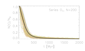
Figure 1: Example for the evolution of the particle number, ensemble with $(N,n)=(200,128)$. The ensemble mean is marked by the thick solid black line.

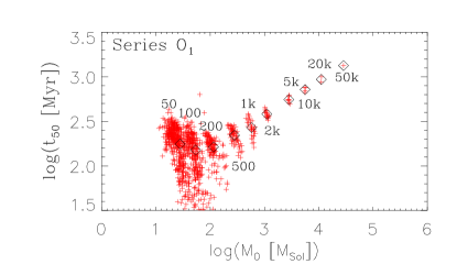
Figure 2: Half-number times versus initial mass for all runs of Series $O_{1}$. The particle numbers are marked by labels. The mean values are marked by diamonds.

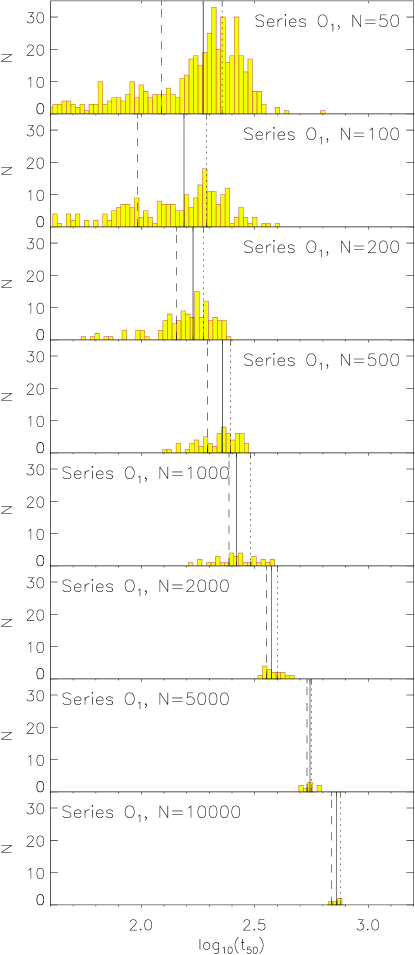
Figure 3: Distributions of half-number times $t_{50}$ for the low-$N$ ensembles of series $O_{1}$. The binsize is $0.02$ dex in $\log_{10}(t_{50})$. The ensemble median $Q_{50}$ is marked by the solid black line. The dotted and dashed lines mark the $30$% and $70$% quantiles $Q_{30}$ and $Q_{70}$ of the corresponding distribution, respectively.

In Figure 4 we compare the evolution of the half-mass radius as function of relative mass loss $M(t)/M_{0}$ in terms of $\lambda$ for different series. This shape parameter $\lambda$ increases during the evolution similar to the result of Fukushige & Heggie (1995) and it is independent of $N$. There is a clear separation of the different series showing that there is a memory of the initial relative size of the half-mass radius.

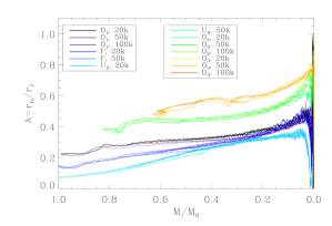
Figure 4: Evolution of the half-mass Roche volume filling factor $\lambda$ as a function of the bound mass $M/M_{0}$.

4.2 Mass loss

The left-hand side of Figure 5 shows the time evolution of the arithmetic ensemble mean of the normalized particle number $N(t)/N_{0}$ within three times the Jacobi radius, which we defined to be bound.

All curves decline monotonically as the simulated star clusters lose mass. The moderately Roche volume underfilling series $U_{1}$ and the strongly Roche volume underfilling series $U_{2}$ dissolve slower than the Roche volume filling series $F$. The reason is that they first need a phase of expansion to fill the Roche volume (e.g. Engle 1999). It can be seen that in the moderately Roche volume overfilling series $O_{2}$ the $N$-dependence is much weaker than in the Roche volume overfilling series $O_{1}$. Moreover, in the strongly Roche volume overfilling series $O_{3}$ the $N$-dependence has almost completely vanished. This indicates that two-body relaxation is not responsible for the dissolution.

The right-hand side of Figure 5 shows the time evolution of the arithmetic ensemble mean of the normalized mass $M(t)/M_{0}$ within three times the Jacobi radius. All curves show a strong initial decrease due to the stellar evolution mass loss. The half-mass times are significantly shorter than the half-number times due to the stellar evolution mass loss. As a consequence the binding energy and Roche volume decrease, which depends on the cluster mass, faster than 2-body relaxation, which depends on the number of stars. These differences decrease with increasing Roche volume filling factor.

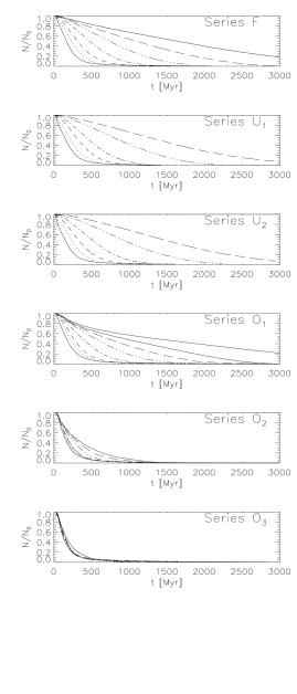
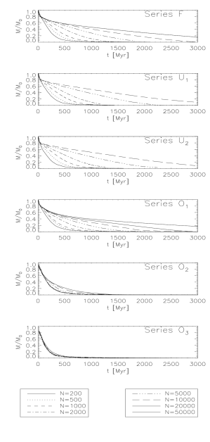
Figure 5: Evolution of the particle number within three times the Jacobi radius (left panels) and cluster mass within three times the Jacobi radius (right panels). From left to right in each panel: $N=200,500,1k,2k,5k,10k,20k,50k$. The sharp initial decrease in the total mass is due to the stellar evolution mass loss.

4.3 Dissolution times

There are four relevant time scales involved in the dissolution of star clusters in the Galactic tidal field: (i) The two-body relaxation time $t_{\rm rx}$, (ii) crossing time $t_{\rm cr}$, (iii) orbital time $t_{\rm orb}$ and (iv) stellar evolution time $t_{\rm stev}$. The first three of them scale as

$$t_{\rm rx}\propto\frac{N}{\ln(\gamma N)}t_{\rm cr},$$ (3)

$$t_{\rm cr}\propto\left(\frac{GM_{\rm cl}}{r_{J}^{3}}\right)^{-1/2}\lambda^{3/2}\propto t_{\rm orb}\lambda^{3/2},$$ (4)

$$t_{\rm orb}\propto\left(\frac{GM_{\rm g}}{R_{g}^{3}}\right)^{-1/2},$$ (5)

where $M_{g}$, $R_{g}$, and $\gamma$, are the the enclosed Galaxy mass, the galactocentric radius, and the factor in the Coulomb logarithm (Giersz & Heggie 1994, 1996), respectively. $r_{J}$ is given by Eqn. (1). We note that we use the initial two-body relaxation time $t_{\rm rx}$ throughout this study and not the current one. The stellar evolution time $t_{\rm stev}$ depends only on the IMF and the metalllicity, which are fixed in our study. For ensembles with large particle numbers $N$ and correspondingly large two-body relaxation times $t_{\rm rx}$ the mass loss due to stellar evolution is clearly distinguishable from the two-body relaxation driven evolution and becomes important with respect to it as can be seen in right-hand side panels of Figure 5.

Figure 6: Half-number times in Myr as functions of $N/\ln(0.02N)$ (dots) and straight-line fits, each using the six lowest-$N$ data points (for $N=200,500,1\mathrm{k},2\mathrm{k},5\mathrm{k},10\mathrm{k}$) to obtain the slopes in the low-$N$ OC limit. The results of a few $\varphi$-grape+gpu simulations are also shown. The $\varphi$-grape+gpu simulation with $1$ million particles belongs to series $O_{1}$. The weights and error bars are calculated from the quantiles $Q_{30,N}$, $Q_{50,N}$ and $Q_{70,N}$ (see text and Eqns. (8) - (10)).

Table 3: The slopes $x_{50}$.

Ser.	$\gamma$	$F$	$U_{1}$	$U_{2}$	$O_{1}$	$O_{2}$	$O_{3}$
$x_{50}$	0.02	0.708	0.843	0.872	0.573	0.238	0.100
$x_{50}$	0.11	0.630	0.752	0.764	0.494	0.212	0.100

Figure 6 shows that, in the low-$N$ regime of OCs, the half-number time $t_{50}$ scales directly with a power $x_{50}(\gamma,\lambda^{\prime})$ of the two-body relaxation time $t_{\rm rx}$. Figure 6 also shows the corresponding straight-line fits for the determination of $x_{50}(\gamma,\lambda^{\prime})$. The 6 lowest-$N$ data points of the nbody6tid ensembles have been used for the fitting of power laws. For the least-squares-fitting, we used the mpfit package in idl (Markwardt 2009; Moré 1978, for the Levenberg-Marquardt algorithm).

We find in this study for the half-number time $t_{50}$ the approximate expression

$$\frac{t_{50}}{T}\approx\left[\frac{1}{C}\frac{N}{\ln(\gamma N)}\right]^{x_{50}(\gamma,\lambda^{\prime})}$$ (6)

with $T\approx 125\ \mathrm{Myr}\propto t_{\rm orb}$ and $C=80-100$. The exponents

$$x_{50}=\frac{d\log t_{50}}{d\log t_{\rm rx}}$$ (7)

for the half-number times are given in the legend of Figure 6 and Table 3, and they are plotted in Figure 7 against the Roche volume filling factor.

The upper and lower errors in Figures 6, 8 and 9 are given by

$$\Delta^{+}\log_{10}t_{i,N} = \log_{10}(Q_{70,i,N})-\log_{10}(Q_{50,i,N}),$$ (8)

$$\Delta^{-}\log_{10}t_{i,N} = \log_{10}(Q_{50,i,N})-\log_{10}(Q_{30,i,N}),$$ (9)

where $Q_{30,N}$, $Q_{50,N}$ and $Q_{70,N}$ are 30%, 50% and 70% quantiles of the corresponding distribution of dissolution times $t_{i}$. The quantiles have been calculated with an idl routine by Hong, Schlegel & Grindlay (2004). The weights used in the fitting procedure are given by

$$w_{i,N}=1/\left[|\Delta^{+}\log_{10}t_{i,N}|+|\Delta^{-}\log_{10}t_{i,N}|\right]^{2}.$$ (10)

The dependence of $x_{50}(\gamma,\lambda^{\prime})$ on the 99% Roche volume filling factor $\lambda^{\prime}$ and the $\gamma$ factor in the Coulomb logarithm can be seen in Figure 7. We calculated the scaling exponents for two different values of the $\gamma$ parameter in the Coulomb logarithm: $\gamma=0.02$ (Giersz & Heggie 1996, multi-mass case) and $\gamma=0.11$ (Giersz & Heggie 1994, equal-mass case only for comparison) to show the difference between these two cases.

Figure 7: Exponent $x_{50}$ from Eqn. (6) as a function of $\lambda^{\prime}=r_{99\%}/r_{J}$. Thick dots: $\gamma=0.02$; thin dots: $\gamma=0.11$.

	$t_{20}$	$t_{50}$	$t_{80}$
$F$
$U_{2}$
$O_{1}$
$O_{2}$

Figure 8: Example fits. From left to right: For $t_{20}$, $t_{50}$, $t_{80}$. From top to bottom: For Series $F,U_{2},O_{1},O_{2}$ . The fits of $t_{20}$ can be biased due to stellar evolution mass loss. We used $\gamma=0.02$ in the Coulomb logarithm. The weights and error bars are calculated from the quantiles $Q_{30,N}$, $Q_{50,N}$ and $Q_{70,N}$ (see text and Eqns. (8) - (10)).

Figure 9: Top panel: Scaling exponents $x_{i}=d\log(t_{\rm i})/d\log(t_{\rm rh})$. The time $t_{i}$ is defined as the time when the cluster has lost $i\%$ of its initial particle number. We used a median smoothing with a smoothing width of 11 in i. Bottom panel: The corresponding $\chi^{\prime 2}_{red,i}$ values. For low i we find large $\chi^{\prime 2}_{red,i}$ due to the stellar evolution mass loss. The half-number time seems to be a robust measure with respect to the $\chi^{\prime 2}_{red,i}$ values. Thick lines: $\gamma=0.02$; thin lines: $\gamma=0.11$. The weights are calculated from the quantiles $Q_{30,N}$, $Q_{50,N}$ and $Q_{70,N}$ (see text and Eqn. (10)).

Figure 8 shows example fits for the times $t_{20}$, $t_{50}$ (half-number time) and $t_{80}$ for Series $F,U_{2},O_{1},O_{2}$. Here we used only $\gamma=0.02$ in the Coulomb logarithm. For the least-squares-fitting, we used the mpfit package in idl (Markwardt 2009; Moré 1978, for the Levenberg-Marquardt algorithm).

Figure 9 shows all scaling exponents

$$x_{i}=\frac{d\log(t_{i})}{d\log(t_{\rm rx})}$$ (11)

for $i=1-90$ (in percent), together with the corresponding $\chi^{2}$ values. The time $t_{i}$ is defined as the time when the cluster has lost $i\%$ of its initial particle number. We calculated the scaling exponents for two different values of the $\gamma$ parameter in the Coulomb logarithm. We used

$$\chi^{\prime 2}_{red,i}=\frac{1}{N_{\rm dof}}\sum_{k=1}^{N_{\rm dof}}((y_{i,k}-f_{i,k})^{2}\times|w_{i,k}|)$$ (12)

with the weights of Eqn. (10), where $f_{i,k}$ is the value of the fitted power law function Eqn. (6), the $y_{i,k}$ are the data and $N_{\rm dof}$ is the number of degrees of freedom (Markwardt 2009). From Figure 9 we can see that the power law index $x_{i}$ is a weak function of the mass loss fraction. The $\chi^{\prime 2}_{red,i}$ is not easy to interpret since the quantiles of the corresponding statistic with the weights of Eqn. (10) are not known. However, one can gain an insight regarding the relative behaviour of $\chi^{\prime 2}_{red,i}$ for different $t_{\rm i}$’s. It can be seen that $t_{\rm 50}$ is a robust measure for the dissolution time.

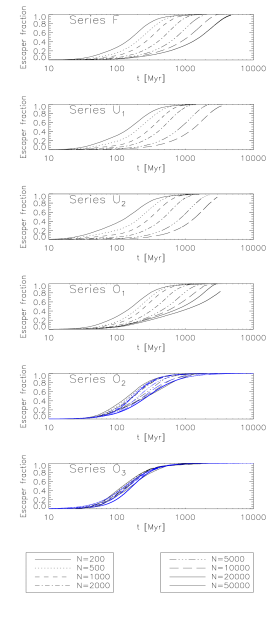
Figure 10: Evolution of the escaper fraction. From left to right in each panel: $N=200,500,1k,2k,5k,10k,20k,50k$ and fits with Eqn. (14). The time axis has been switched from linear to logarithmic. The log-logistic growth occurs in the Roche volume overfilling limit. The corresponding fits are shown (blue lines).

4.4 Log-logistic growth

Table 4: Averaged parameters $(\log_{10}(t_{50}\ [\mathrm{Myr}]),\kappa)$ from fits with Equation (15).

Series	$\log_{10}(t_{50}\ [\mathrm{Myr}])$	$\kappa$
$O_{2}$	$2.30\pm 0.09$	$2.25\pm 0.28$
$O_{3}$	$2.16\pm 0.04$	$2.18\pm 0.20$

Figure 10 shows the time evolution of the escaper fraction $N_{e}(t)/N_{0}=1-N(t)/N_{0}$ with a logarithmic time axis, where $N(t)$ (and $N_{0}$) are taken to be the current (initial) particle number within three times the Jacobi radius.

In the Roche volume overfilling limit the evolution of the escaper fraction can, at least empirically, be approximately described by a log-logistic differential equation in logarithmic time,

$$\frac{d\ln N_{e}}{d\ln t}=\kappa\left(1-\frac{N_{e}}{N_{0}}\right)=\kappa\frac{N}{N_{0}}.$$ (13)

The solution is given by

$$\frac{N_{e}(t)}{N_{0}}=\frac{t^{\kappa}}{t_{50}^{\kappa}+t^{\kappa}}.$$ (14)

The evolution of $N(t)/N_{0}$ can then be described by the law

$$\frac{N(t)}{N_{0}}=\frac{t_{50}^{\kappa}}{t_{50}^{\kappa}+t^{\kappa}}.$$ (15)

The best-fit exponent $\kappa$ and the best-fit half-number time $t_{50}$ can be determined for the parameter space covered in this study. Table 4 shows the parameters of least-quares fits with the Equation

$$\log t=\log t_{50}+\frac{1}{\kappa}\log\left(\frac{N_{e}/N_{0}}{1-N_{e}/N_{0}}\right).$$ (16)

For the least-squares-fitting, we used the mpfit package in idl (Markwardt 2009; Moré 1978, for the Levenberg-Marquardt algorithm). The fits are shown in the two lowest panels on the right-hand side of Figure 10 (for series $O_{2}$ and $O_{3}$). For the series shown in the upper panels we suspect a transition from log-logistic to logistic with some other contribution from left to right, where the factor $1/t$ is due to the stellar evolution (Lamers, Baumgardt & Gieles 2010) and the other contribution is due to the relaxation-driven evolution.

There are two competing processes for populating the potential escaper reservoir above the critical Jacobi energy. Firstly, scattering by stellar encounters scales with the relaxation time and depends on the particle number $N$. Secondly, cluster mass loss by stellar evolution and by escaping stars lowers the cluster potential well and lifts the critical Jacobi energy, which shifts new stars above the critical value. The fractional mass loss rate is independent of $N$ and results in a particle loss rate proportional to $N$, to the number of escapers $N_{e}$ and via stellar evolution to $1/t$ (Lamers, Baumgardt & Gieles 2010). For the overfilling clusters (series $O_{2}$, $O_{3}$) two-body encounters are negligible leading to the log-logistic behaviour. For the more concentrated clusters, where two-body encounters play an important role, the interplay of the different timescales is discussed in detail in Lamers, Baumgardt & Gieles (2010). Only for very large $N$, where the relaxation time is very long, the factor $1/t$ by stellar evolution in the dissolution timescale becomes relevant again. This leads to a reduction of $t_{50}$ with respect to the power law dependence derived in Eqn. (6) for small filling factors.

5 Conclusions

We have carried out a parameter study of open star clusters with the parameters $(N,\lambda=r_{t}/r_{J})$. We have found the following results:

1. The $N$-dependence of the dissolution time in units of the two-body relaxation time is well fitted by a power law. The power law index is a function of the Roche volume filling factor $\lambda$ and the $\gamma$ factor in the Coulomb logarithm. It decreases with increasing $\lambda$ with the limiting value of zero in the overfilling limit. Particularly in the underfilling limit, the power law index has been found to depend on the value of the $\gamma$ parameter adopted in the Coulomb logarithm.

2. Our study suggests that open star clusters in the Roche volume overfilling regime dissolve mainly due to the changing cluster potential by lifting stars above the decreasing critical Jacobi energy. We call this mechanism “mass-loss driven dissolution” in contrast to the “two-body relaxation driven dissolution” which occurs from the Roche volume underfilling regime up to the Roche volume filling case (see also Whitehead et al. 2013, based on simpler models).

3. In the Roche volume overfilling limit the escaper fraction $N_{e}(t)/N_{0}$ obeys, at least empirically, approximately a log-logistic differential equation in logarithmic time.

We make the following remarks:

1. The mass-loss driven dissolution provides a mechanism, which is responsible for the dissolution of OCs which have survived the gas expulsion phase with a relatively large initial half-mass radius as observed for example in the Pleiades cluster (Converse & Stahler 2010). It is a viable mechanism besides the dissolution due to encounters with giant molecular clouds (Wielen 1971, 1985).

2. The mass-loss driven dissolution in combination with a large scatter in Roche volume filling factors (Ernst & Just 2013) also naturally explains the large scatter in the lifetimes of open clusters (Wielen 1971). In a future paper we plan to investigate the impact of the newly found $N$-independence of the dissolution timescale for the overfilling clusters on the CFR using the observed mass-age distribution of OCs in the solar neighbourhood.

3. Due to the intricacy of the problem a detailed theory of mass-loss driven dissolution, which explains the transition from the over- to underfilling limits in terms of the dependence of $x_{50}$ on $\lambda$ as shown in Figure 7 has not yet been developed and is beyond the scope of the present experimental study.

Appendix A Resonance condition

It is possible to write down a resonance condition (Ernst & Just 2013),

$$\frac{m}{n} = \frac{\Omega}{\omega_{\rm res}}=\left(\frac{4-\beta_{C}^{2}}{2}\right)^{1/2}\left(\frac{r_{\rm res}}{r_{J}}\right)^{3/2},$$ (17)

where $m$ and $n$ are natural numbers and the orbital frequencies $\omega_{\rm res}=\omega(r_{\rm res})$ and $\Omega=2\pi/t_{\rm orb}$ are related to the orbital time of a star in the star cluster and the orbital time of the star cluster on a circular orbit around the galaxy, respectively. $\beta_{C}$ is the ratio between epicyclic and circular frequency and $r_{\rm res}$ is a resonance radius. For a flat rotation curve we have $\beta_{C}=\sqrt{2}$. For the Milky Way model with the parameters given in Table 1 we have $\beta_{C}\approx 1.37$ at $R_{g}=8$ kpc. Therefore at certain values of $\lambda=r_{h}/r_{J}$ resonance effects may occur and play a role in the evolution.

The central periodic orbit in the largest regular (i.e. non-chaotic) island in the Poincaré surfaces of section at the critical Jacobi energy has $(r_{\rm res}/r_{J})=0.345$. This island corresponds to quasiperiodic retrograde orbits (Fukushige & Heggie 2000; see also Ernst et al. 2008). It may be that the corresponding resonance is linked with the properties of star clusters and connected with the occurence of two discrete types of star clusters, open and globular clusters. Moreover, the location of the resonance may be used to calibrate the relation (17) more precisely for star clusters, i.e. to determine $r_{\rm res}$ as a function of $r_{h}$.

Appendix B Stability curve

Figure 11: Stability curve for a Plummer model and King models. Value of $r_{h}/r_{V}$ for $W_{0}=11$ by Gürkan and Freitag, priv. comm.

In connection with the Roche volume filling factor a stability curve can be derived for star clusters. Such a curve has been derived for the first time in Fukushige & Heggie (1995, their Eqn. 28; see also their Figure 13) and may therefore be called the “Fukushige-Heggie stability curve” for star clusters. The Jacobi energy of a typical star at the half-mass radius is given by

$$e_{J,h}=\frac{K}{M_{\rm cl}}+\frac{W}{M_{\rm cl}}-\frac{1}{2}\frac{GM}{r_{h}}\lambda^{3}\\$$ (18)

with $\lambda=r_{h}/r_{J}$, where $K$ and $W$ are the kinetic and potential energies, respectively. The critical Jacobi energy is given by

$$e_{\rm J,crit}=-\frac{3}{2}\frac{GM_{\rm cl}}{r_{J}}.$$ (19)

We obtain for a Plummer model with

$$K=-\frac{W}{2}=\frac{3\pi}{64}\frac{GM_{\rm cl}^{2}}{r_{\rm Pl}},$$ (20)

and $r_{h}/r_{\rm Pl}\approx 1.305$ the stability curve

$$\frac{e_{J,h}-e_{J,\rm crit}}{e_{J,\rm crit}}\approx\frac{1.305\cdot\pi}{32\lambda}+\frac{\lambda^{2}}{3}-1$$ (21)

For a King model with $W_{0}=6$ we have

$$K=-E=\frac{GM_{\rm cl}^{2}}{4r_{V}}$$ (22)

with $r_{h}/r_{V}\approx 0.804$ (Half-mass radius in $N$-body units $G=M_{\rm cl}=-4E=1$, Gürkan, Freitag & Rasio 2004, Table 1), where $E$ is the total energy. We obtain the stability curve

$$\frac{e_{J,h}-e_{J,\rm crit}}{e_{J,\rm crit}}\approx\frac{0.804}{6\lambda}+\frac{\lambda^{2}}{3}-1$$ (23)

The stability curves in Eqns. (21) and (23) are shown in Figure 11 for a Plummer model and 3 King models and may be also connected with the occurence of two discrete types of star clusters, open and globular clusters. The value of this function measures the relative Jacobi energy difference between a typical star at the half-mass radius and the critical Jacobi energy. Note that Eqn. (19) and the virial relations in Eqns. (20) and (22) break down for large $\lambda$, i.e. only the first zero at small $\lambda$ may be of physical significance. We expect relaxation driven dissolution in the regime to the left of the first zero and mass-loss driven dissolution in the regime to the right of the first zero.