A combined finite volume - finite element scheme for a dispersive shallow water system

Abstract.

We propose a variational framework for the resolution of a non-hydrostatic Saint-Venant type model with bottom topography. This model is a shallow water type approximation of the incompressible Euler system with free surface and slightly differs from the Green-Nagdhi model, see [12] for more details about the model derivation.

The numerical approximation relies on a prediction-correction type scheme initially introduced by Chorin-Temam [16] to treat the incompressibility in the Navier-Stokes equations. The hyperbolic part of the system is approximated using a kinetic finite volume solver and the correction step implies to solve a mixed problem where the velocity and the pressure are defined in compatible finite element spaces.

The resolution of the incompressibility constraint leads to an elliptic problem involving the non-hydrostatic part of the pressure. This step uses a variational formulation of a shallow water version of the incompressibility condition.

Several numerical experiments are performed to confirm the relevance of our approach.

Inria, EPC ANGE, Rocquencourt- B.P. 105, F78153 Le Chesnay cedex, France

CEREMA, EPC ANGE, 134 rue de Beauvais, F-60280 Margny-Les-Compiegne , France

Sorbonne Universités, UPMC Univ Paris 06, UMR 7598, Laboratoire Jacques-Louis Lions, F-75005, Paris, France

CNRS, UMR 7598, Laboratoire Jacques-Louis Lions, F-75005, Paris, France

(Communicated by the associate editor name)

1. Introduction

Starting from the incompressible Euler or Navier-Stokes system, the hydrostatic assumption consists in neglecting the vertical acceleration of the fluid. More precisely – and with obvious notations – the momentum along the vertical axis of the Euler equation

$$\frac{\partial w}{\partial t}+u\frac{\partial w}{\partial x}+w\frac{\partial w}{\partial z}+\frac{\partial p}{\partial z}=-g,$$

reduces in the hydrostatic context to

$$\frac{\partial p}{\partial z}=-g.$$ (1)

Such an assumption produces important consequences over the structure and complexity of the model. Indeed, Eq. (1) implies that the pressure $p$ is no longer the Lagrange multiplier of the incompressibility constraint and $p$ can be expressed, for free surface flows, as a function of the water depth of the fluid. Therefore, the hydrostatic assumption implies that the resulting model, even though it describes an incompressible fluid, has common features with models arising in compressible fluid mechanics.

In geophysical problems, the hydrostatic assumption coupled with a shallow water type description of the flow is often used. Unfortunately, these models do not represent phenomena containing dispersive effects for which the non-hydrostatic contribution cannot be neglected. And more complex models have to be considered to take into account this kind of phenomena, together with numerical methods able to discretize the high order derivative terms coming from the dispersive effects. Many shallow water type dispersive models have been proposed such as KdV, Boussinesq, Green-Naghdi, see [21, 14, 6, 30, 31, 27, 19, 26, 2, 3, 13]. The modeling of the non-hydrostatic effects for shallow water flows does not raise insuperable difficulties but their discretization is more tricky. Numerical techniques for the approximaion of these models have been recently proposed [15, 11, 28].

The model studied in the present paper has been derived and studied in [12]. Its numerical approximation based on a projection-correction strategy [16] is described in [1]. In [1], the discretization of the elliptic part arising from the non-hydrostatic terms is carried out in a finite difference framework. It is worth noticing that the numerical scheme given in [1] is endowed with robustness and stability properties such as positivity, well-balancing, discrete entropy and wet/dry interfaces treatment.

The main contents of this paper is the derivation and validation of the correction step in a variational framework. Since the derivation in a 2d context of the model proposed in [12] does not raise difficulty, the results depicted in this paper pave the way for a discretization of the 2d model over an unstructured mesh, and we will often maintain general notations as far as possible.

Notice that the non-hydrostatic model we consider slightly differs from the well-known Green-Naghdi model [21] but the numerical approximation proposed in this paper can also be used for the numerical approximation of the Green-Naghdi system.

Let $\Omega\subset\mathbb{R}$, be a 1d domain (an interval) and $\Gamma=\Gamma_{in}\cup\Gamma_{out}$ its boundary (see figure 1). The non-hydrostatic model derived in  [12, 1] reads

$$\frac{\partial H}{\partial t}+\frac{\partial H\overline{u}}{\partial x} = 0,$$ (2)

$$\frac{\partial H\overline{u}}{\partial t}+\frac{\partial}{\partial x}(H\overline{u}^{2}+g\frac{H^{2}}{2}+H\overline{p}_{nh}) = -(gH+2\overline{p}_{nh})\frac{\partial z_{b}}{\partial x},$$ (3)

$$\frac{\partial H\overline{w}}{\partial t}+\frac{\partial H\overline{w}\overline{u}}{\partial x} = 2\overline{p}_{nh},$$ (4)

$$\frac{\partial H\bar{u}}{\partial x}-\bar{u}\frac{\partial(H+2z_{b})}{\partial x}+2\bar{w} = 0,$$ (5)

where $H$ is the water depth, $z_{b}$ the topography and $p_{nh}$ the non-hydrostatic part of the pressure. The variables denoted with a bar recall that this model is obtained performing an average along the water depth of the incompressible Euler system with free surface. The velocity field is denoted $\mathbb{\bar{u}}=(\bar{u},\bar{w})^{t}$ with $\bar{u}$ (resp. $\bar{w}$) the horizontal (resp. vertical) component.

We denote $\eta=H+z_{b}$ the free surface of the fluid. In addition, we give the following notations

$$\mathbb{n}=\left(\begin{array}[]{ccc}n\\ 0\end{array}\right),$$ (8)

with $n$ the unit outward normal vector at $\Gamma$ (in 1d, $n=\pm$ 1), $\mathbb{n}$ represents the unit outward normal vector of the domain covered by the fluid, namely $\Omega\times[z_{b},\eta]$. We also consider the gradient operator

$$\nabla_{0}=\left(\begin{array}[]{ccc}\frac{\partial}{\partial x}\\ 0\end{array}\right).$$ (11)

Figure 1. Notations and domain definition.

The smooth solutions of the system (2)-(5) satisfy moreover an energy conservation law

$$\frac{\partial\bar{E}}{\partial t}+\frac{\partial}{\partial x}\left(\bar{u}\left(\bar{E}+\frac{g}{2}H^{2}+H\bar{p}_{nh}\right)\right)=0,$$ (12)

with

$$\bar{E}=\frac{H\left(\bar{u}^{2}+\bar{w}^{2}\right)}{2}+\frac{gH\left(\eta+z_{b}\right)}{2}.$$ (13)

Note that (5) represents a shallow water version of the divergence free constraint, for which the non hydrostatic pressure $\bar{p}_{nh}$ plays the role of a Lagrange multiplier. Notice that considering $\bar{p}_{nh}=0$ and neglecting (4), the system (2)-(3),(5) reduces to the classical Saint-Venant system.

The paper is organized as follows. First we give a rewriting of the model and we present the prediction-correction method, the main part being the variationnal formulation of the correction part. Then in Section 3, we detail the numerical approximation. Finally, in Section 4, numerical simulations validating the proposed discretization techniques are presented.

2. The projection scheme for the non-hydrostatic model

Projection methods have been introduced by A. Chorin and R. Temam [33] in order to compute the pressure for incompressible Navier-Stokes equations. These methods, based on a time splitting scheme, have been widely studied and applied to treat the incompressibility constraint (see [24, 35, 34]). We develop below an analogue of this method for shallow water flow. In order to describe the fractional time step method we use, we propose a rewritting of the model (2)-(5).

2.1. A rewritting

Let us introduce the two operators $\nabla_{\!sw}\,$ and ${\rm div}_{\!sw}\,$ defined by

$$\nabla_{\!sw}\,f = \left(\begin{matrix}H\frac{\partial f}{\partial x}+f\frac{\partial(H+2z_{b})}{\partial x}\\ -2f\end{matrix}\right),$$ (14)

$${\rm div}_{\!sw}\,(\mathbb{v}) = \frac{\partial Hv_{1}}{\partial x}-v_{1}\frac{\partial(H+2z_{b})}{\partial x}+2v_{2},$$ (15)

with $\mathbb{v}=(v_{1},v_{2})^{t}$. We assume for a while that $f$ and $\mathbb{v}$ are smooth enough. The shallow water form of the divergence operator ${\rm div}_{\!sw}\,$ (resp. of the gradient operator $\nabla_{\!sw}\,$) corresponds to a depth averaged version of the divergence (resp. gradient) appearing in the incompressible Euler and Navier-Stokes equations. Notice that the two operators $\nabla_{\!sw}\,$, ${\rm div}_{\!sw}\,$ defined by (14)-(15) are $H$ and $z_{b}$ dependent and we assume that $H$ and $z_{b}$ are sufficiently smooth functions. One can check that these operators verify the fundamental duality relation

$$\int_{\Omega}{\rm div}_{\!sw}\,(\mathbb{v})f\,dx=-\int_{\Omega}\nabla_{\!sw}\,f\cdot\mathbb{v}\,dx+\left[Hv_{1}\,f\right]_{\Gamma}.$$ (16)

These definitions allow to rewrite the model (2)-(5) as

$$\frac{\partial H}{\partial t}+\frac{\partial H\bar{u}}{\partial x} = 0,$$ (17)

$$\frac{\partial H\mathbb{\bar{u}}}{\partial t}+\frac{\partial}{\partial x}\left(\overline{u}H\overline{\bf u}\right)+\nabla_{0}\left(\frac{g}{2}H^{2}\right)+\nabla_{\!sw}\,\bar{p}_{nh} = -gH\nabla_{0}z_{b},$$ (18)

$${\rm div}_{\!sw}\,(\mathbb{\bar{u}}) = 0,$$ (19)

with $\nabla_{0}$ defined by (11).

The system (17)-(19) can be written in the compact form

$$\frac{\partial X}{\partial t}+\frac{\partial}{\partial x}F(X)+R_{nh} = S(X),$$ (20)

$${\rm div}_{\!sw}\,(\mathbb{\bar{u}}) = 0,$$ (21)

where we denote

$$X=\left(\begin{array}[]{ccc}H\\ H\bar{u}\\ H\bar{w}\\ \end{array}\right),\quad\quad F(X)=\left(\begin{array}[]{ccc}H\bar{u}\\ H\bar{u}^{2}+\frac{g}{2}H^{2}\\ H\bar{u}\overline{w}\\ \end{array}\right),$$ (28)

and

$$R_{nh}=\left(\begin{array}[]{ccc}0\\ \nabla_{\!sw}\,\bar{p}_{nh}\end{array}\right),\quad\quad S(X)=\left(\begin{array}[]{ccc}0\\ -gH\nabla_{0}z_{b}\end{array}\right).$$ (33)

Let be given time steps $\Delta t^{n}$ and note $t^{n}=\sum_{k\leq n}\Delta t^{k}$. As detailed in [1], the projection scheme for system (20)-(21) consists in the following time splitting

$$X^{n+1/2} = X^{n}-\Delta t^{n}\,\frac{\partial}{\partial x}F(X^{n})+\Delta t^{n}\,S(X^{n}),$$ (34)

$$X^{n+1} = X^{n+1/2}-\Delta t^{n}\,R_{nh}^{n+1},$$ (35)

$${\rm div}_{\!sw}\,{\mathbb{\bar{u}}^{n+1}} = 0,$$ (36)

with $\mathbb{\bar{u}}^{n+1}=\left(\frac{(H\bar{u})^{n+1}}{H^{n+1}},\frac{(H\bar{w})^{n+1}}{H^{n+1}}\right)^{t}$.

The first two equations of (34) consist in the classical Saint-Venant system with topography and the third equation is an advection equation for the quantity $H\bar{w}$. Equations (35)-(36) describe the correction step allowing to determine the non hydrostatic part of the pressure $p_{nh}^{n+1}$ and hence giving the corrected state $X^{n+1}$. The numerical resolution of (34) – especially the first two equations – has received an extensive coverage and efficient and robust numerical techniques exist, mainly based on finite volume approach, see [8, 5]. The derivation of a robust and efficient numerical technique for the resolution of the correction step (35)-(36) is the key point. A strategy based on a finite difference approach has been proposed, studied and validated in [1]. Unfortunately, the finite difference framework does not allow to tackle situations with unstructured meshes in 2 or 3 dimensions. It is the key point of this paper to propose a variational formulation of the correction step coupled with a finite volume discretization of the prediction step.

The time discretization in the numerical scheme described above corresponds to a fractional time step strategy with a first order Euler scheme, explicit for the hyperbolic part and implicit for the elliptic part. For hyperbolic conservation laws, the second-order accuracy in time is usually recovered by the Heun method [7, 8] that is a slight modification of the second order Runge-Kutta method. More precisely, for a dynamical system written under the form

$$\frac{\partial y}{\partial t}=F(y),$$ (37)

the Heun scheme consists in defining $y^{n+1}$ by

$$y^{n+1}=\frac{y^{n}+\tilde{y}^{n+2}}{2},$$ (38)

with

$$\tilde{y}^{n+1}=y^{n}+\Delta t^{n}F(y^{n}),$$

$$\tilde{y}^{n+2}=\tilde{y}^{n+1}+\Delta t^{n}F(\tilde{y}^{n+1}).$$

The model we have to discretize has the general form

$$\frac{\partial X}{\partial t}=F(X,p),$$ (39)

$$B(X)=0,$$

and we propose the numerical scheme

$$X^{n+1}=\frac{X^{n}+\tilde{X}^{n+2}}{2},$$ (40)

with the two steps defined by

$$\tilde{X}^{n+1}=X(t^{n})+\Delta t^{n}F(X^{n},\tilde{p}^{n+1}),$$ (41)

$$B(\tilde{X}^{n+1})=0,$$ (42)

and

$$\tilde{X}^{n+2}=\tilde{X}^{n+1}+\Delta t^{n}F(\tilde{X}^{n+1},\tilde{p}^{n+2}),$$ (43)

$$B(\tilde{X}^{n+2})=0,$$ (44)

where $\tilde{p}^{n+1}$ and $\tilde{p}^{n+2}$ are the solutions of the elliptic equations derived from the divergence free constraints (42) and (44) respectively. Notice that (41) is a compact form of the fractional scheme (34)-(35) where the intermediate step no more appears.

It is easy to prove the scheme (40) is second order accurate. Indeed assuming $F$ and $B$ are enough smooth, we have

$$X(t^{n}+\Delta t^{n})=X(t^{n})+\Delta t^{n}\dot{X}(t^{n})+\frac{(\Delta t^{n})^{2}}{2}\ddot{X}(t^{n})+{\mathcal{O}}\bigl{(}(\Delta t^{n})^{3}\bigr{)},$$

or equivalently using (39)

$$X(t^{n}+\Delta t^{n})=X(t^{n})+\Delta t^{n}F(X(t^{n}),p(t^{n}))\\ +\frac{(\Delta t^{n})^{2}}{2}\left(F(X(t^{n}),p(t^{n}))\frac{\partial F(X(t^{n}),p(t^{n}))}{\partial X}+\frac{\partial F(X(t^{n}),p(t^{n}))}{\partial p}\frac{\partial p(t^{n})}{\partial t}\right)+{\mathcal{O}}\bigl{(}(\Delta t^{n})^{3}\bigr{)}.$$ (45)

Now from (41) and (43), we get

$$\tilde{X}^{n+2} = X^{n}+\Delta t^{n}F(X^{n},\tilde{p}^{n+1})+\Delta t^{n}F(\tilde{X}^{n+1},\tilde{p}^{n+2})$$ (46)

$$= X^{n}+2\Delta t^{n}F(X^{n},\tilde{p}^{n+1})$$

$$+(\Delta t^{n})^{2}\left(F(X^{n},\tilde{p}^{n+1})\frac{\partial F(X^{n},\tilde{p}^{n+1})}{\partial X}+\frac{\partial F(X^{n},\tilde{p}^{n+1})}{\partial p}\frac{\partial\tilde{p}^{n+1}}{\partial t}\right)$$

$$+{\mathcal{O}}\bigl{(}(\Delta t^{n})^{3}\bigr{)}.$$

Using (40), we see that relations (45) and (46) are equivalent up to third order terms.

2.2. The correction step

In this part, we consider we have at our disposal a space discretization of Eq. (34) solving the hydrostatic part of the model and we focus on the correction step (35)-(36).

2.2.1. Variational formulation

The correction step (35)-(36) writes,

$$H^{n+1} = H^{n+1/2},$$ (47)

$$(H\mathbb{u})^{n+1}+\Delta t^{n}\nabla_{\!sw}\,{p}_{nh}^{n+1} = (H\mathbb{u})^{n+1/2},$$ (48)

$${\rm div}_{\!sw}\,(\mathbb{u}^{n+1}) = 0.$$ (49)

For the sake of clarity, in the following we will drop the notation with a bar and we denote $p$ instead of $\bar{p}_{nh}$. Likewise we drop the superscript ⁿ⁺¹ for the corrected states.

Equations (48)-(49) is a mixed problem in velocity/pressure, its approximation leads to the variational mixed problem

Find ${p}\in Q$, $\mathbb{u}\in V_{0}$ with

$$Q=\{q\in L^{2}(\Omega)|\nabla_{\!sw}\,q\in(L^{2}(\Omega))^{2}\},$$ (50)

and

$$V_{0}=\{{\bf v}=(v_{1},v_{2})\in(L^{2}(\Omega))^{2}|{\rm div}_{\!sw}\,(\mathbb{v})\in L^{2}(\Omega),{v_{1}}_{|\Gamma}=0\},$$ (51)

such that

$$\int_{\Omega}\left(H\mathbb{u}+\Delta t^{n}\nabla_{\!sw}\,p\right)\cdot\mathbb{v}\,dx = \int_{\Omega}(H\mathbb{u})^{n+1/2}\cdot\mathbb{v}\ dx,\quad\forall\,\mathbb{v}\in V_{0},$$ (52)

$$\int_{\Omega}{\rm div}_{\!sw}\,(\mathbb{u})q\,dx = 0,\quad\forall q\in Q.$$ (53)

Introducing the bilinear forms

$$a(\mathbb{u},\mathbb{v}) = \int_{\Omega}H\mathbb{u}\cdot\mathbb{v}\,dx,\quad\forall\,\mathbb{u},\mathbb{v}\in V_{0},$$

$$b(\mathbb{v},q) = -\int_{\Omega}{\rm div}_{\!sw}\,(\mathbb{v})q\,dx,\quad\forall\mathbb{v}\in V_{0},\forall\,q\in Q,$$

the problem (52)-(53) becomes:
Find $p\in Q$ and $\mathbb{u}\in V_{0}$ such that

$$\frac{1}{\Delta t^{n}}a(\mathbb{u},\mathbb{v})+b(\mathbb{v},p) = \frac{1}{\Delta t^{n}}a(\mathbb{u}^{n+1/2},\mathbb{v}),\quad\forall\mathbb{v}\in V_{0},$$ (54)

$$b(\mathbb{u},q) = 0,\quad\forall q\in Q.$$ (55)

2.2.2. The pressure equation

Formally, we take $\mathbb{v}$ in the form $\mathbb{v}=\frac{\nabla_{\!sw}\,q}{H}$ with $q\in Q_{0}$ and

$$Q_{0}=\{q\in Q\,q|_{\Gamma}=0\}.$$

Then, with (16) and (55), we get

$$a(\mathbb{u,\mathbb{v}}) = \int_{\Omega}u\cdot\nabla_{\!sw}\,qdx$$

$$= -\int_{\Omega}{\rm div}_{\!sw}\,(\mathbb{u})\cdot qdx$$

$$= 0.$$

If we introduce the shallow water version of the Laplacian operator $\Delta_{sw}\,$

$$\Delta_{sw}\,p={\rm div}_{\!sw}\,\left(\frac{1}{H}\nabla_{\!sw}\,p\right),$$

it is natural to consider the new variational formulation:

Find $\mathbb{u}\in V,p\in Q_{0,sw}$ such that

$$\frac{1}{\Delta t^{n}}a(\mathbb{u},\mathbb{v})+(\mathbb{v},\nabla_{\!sw}\,p) = \frac{1}{\Delta t^{n}}a(\mathbb{u}^{n+1/2},\mathbb{v})\quad\forall\mathbb{v}\in V,$$ (56)

$$\left(\Delta_{sw}\,p,q\right) = \frac{1}{\Delta t^{n}}\left({\rm div}_{\!sw}\,(\mathbb{u}^{n+1/2}),q\right),\quad\forall q\in Q_{0,sw},$$ (57)

with $Q_{0,sw}=\{q\in Q_{0}|{\rm div}_{\!sw}\,\left(\frac{\nabla_{\!sw}\,q}{H}\right)\in L^{2}(\Omega)\}$.

From (57), we deduce

$$\Delta_{sw}\,(p)=\frac{1}{\Delta t^{n}}{\rm div}_{\!sw}\,(\mathbb{{u}}^{n+1/2}).$$ (58)

The resolution of the equation (58) allows to update the velocity at the correction step (48).

Notice that the equation (58) is equivalent to apply the operator ${\rm div}_{\!sw}\,$ to the equation (35) and to use the shallow water free divergence (36) to eliminate $\mathbb{u}$.

Remark 1.

Taking the functional spaces $V$ and $Q_{0,sw}$, the problem (56)-(57) is not equivalent to the problem (54)-(55).

Remark 2.

Notice that Eq. (58) has the form of a Sturm-Liouville type equation.

2.2.3. Inf-sup condition

To ensure that the saddle problem (54)-(55) is well posed, the Babuska-Brezzi [9, 32] condition

$$\exists\gamma>0,\quad\gamma<\inf_{q\in Q}\sup_{\mathbb{v}\in V_{0}}\frac{b(\mathbb{v},q)}{||\mathbb{v}||_{V_{0}}||q||_{Q}},$$

has to be satisfied. Denoting by $\mathcal{B}$ the weak operator defined by $\forall v\in V_{0}$, $\mathcal{B}v=b(v,q),\forall q\in Q$, we have

$$\ker\mathcal{B}^{t} = \{q\in Q|\mathcal{B}^{t}q=0\}$$

$$= \{q\in Q|\int_{\Omega}\nabla_{\!sw}\,q\cdot\mathbb{v}\,dx=0\;\forall\mathbb{v}\in V_{0}\}.$$

We assume $H\geq H_{0}>0$. Because of the positivity of $H$, it is obvious that the bilinear form $a$ is coercive. Choosing $\mathbb{v}\in(L^{2}(\Omega))^{2}$ and $q$ such as $\nabla_{\!sw}\,q\in(L^{2}(\Omega))^{2}$, it follows that $\nabla_{\!sw}\,q=0$, then $q=0$ and $\ker\mathcal{B}^{t}={0}$. Indeed, in contrast with Navier-Stokes equations for which the pressure is defined up to an additive constant, the non hydrostatic of the shallow water equations is fully defined. Therefore, the mixed problem (54)-(55) satisfies the inf-sup condition and admits a unique solution.

2.3. Boundary conditions

In this section, we still consider that the hydrostatic part is provided and we study the compatibility of the boundary conditions between the hydrostatic part and the projection part. Therefore, the compatibility between the pressure and velocity at boundary needs to be studied. To this aim, we first provide the conditions required to impose Dirichlet or Neumann pressure at boundary, and then, we couple these conditions with the hydrostatic part.

We consider a more general case taking the space $V$

$$V=\{\mathbb{v}=(v_{1},v_{2})\in(L^{2}(\Omega))^{2}|{\rm div}_{\!sw}\,\mathbb{v}\in L^{2}(\Omega)\},$$

and we introduce the bilinear form

$$c(\mathbb{v},p)=\int_{\Gamma}Hp\,v_{1}\,n\,ds,\quad\forall\mathbb{v}\in V,p\in Q,$$

with $n$ the unit outward normal vector defined by (8). In one dimension, $c(\mathbb{v},p)=(Hpv_{1})|_{\Gamma_{out}}-(Hpv_{1})|_{\Gamma_{in}}$.

Therefore instead of (54)-(55), we consider the problem:
Find $\mathbb{u}\in V$, $p\in Q$ such that,

$$\frac{1}{\Delta t^{n}}a(\mathbb{u},\mathbb{v})+b(\mathbb{v},p) = \frac{1}{\Delta t^{n}}a(\mathbb{u}^{n+1/2},\mathbb{v})+c(\mathbb{v},p),\quad\forall\,\mathbb{v}\in V,$$ (59)

$$b(\mathbb{u},q) = 0,\quad\forall q\in Q.$$ (60)

Notice that ${\rm div}_{\!sw}\,(\mathbb{u})=\nabla_{0}\cdot(H\mathbb{u})+\mathbb{u}\cdot(\mathbb{n_{s}}+\mathbb{n_{b}})$ and $\nabla_{\!sw}\,p=H\nabla_{0}(p)-p(\mathbb{n_{s}}+\mathbb{n_{b}})$ with $\nabla_{0}$ defined by (11) and $\mathbb{n_{s}}$ (resp. $\mathbb{n_{b}}$) the (non-unit) normal vector at the surface (resp. at the bottom)

$$\mathbb{n_{s}}=\left(\begin{array}[]{ccc}-\frac{\partial\eta}{\partial x}\\ 1\end{array}\right),\qquad\mathbb{n_{b}}=\left(\begin{array}[]{ccc}-\frac{\partial z_{b}}{\partial x}\\ 1\end{array}\right).$$

Moreover, we have

$$\int_{\Omega}{\rm div}_{\!sw}\,(\mathbb{u})\;dx=\int_{\Gamma}H{u}\,n\,ds+\int_{\Omega}\mathbb{u}\cdot(\mathbb{n_{s}}+\mathbb{n_{b}})\,dx.$$

Hence, to satisfy the divergence free condition, the velocity $\mathbb{u}$ should verify

$$\int_{\Gamma}H{u}\,n\,ds=-\int_{\Omega}\mathbb{u}\cdot(\mathbb{n_{s}}+\mathbb{n_{b}})\,dx.$$

Dirichlet condition for the pressure

From the variational formulation (54)-(55) of the projection scheme, a natural boundary condition for the pressure is a Dirichlet condition. At $\Gamma_{i},(i=in,out)$, $p|_{\Gamma_{i}}=p_{0}$ then $c(\mathbb{v},p)=\int_{\Gamma_{i}}p_{0}v_{1}n\,ds$ and we take $\mathbb{v}\in V$, $q\in Q_{i}$ with

$$Q_{i} = \{q\in L^{2}(\Omega)|\nabla_{\!sw}\,q\in(L^{2}(\Omega))^{2},q|_{\Gamma_{i}}=0\}.$$

Neumann boundary for the pressure

The Neumann boundary condition for the projection scheme is not natural and to enforce such a condition, the elliptic problem (56)-(57) has to be considered. Taking now $q\in Q_{sw}$, with $Q_{sw}=\{q\in Q|{\rm div}_{\!sw}\,(\frac{\nabla_{\!sw}\,p}{H})\in L^{2}(\Omega)^{2}\}$, the problem is rewritten

$$\frac{1}{\Delta t^{n}}a(\mathbb{u},\mathbb{v})+(\mathbb{v},\nabla_{\!sw}\,p) = \frac{1}{\Delta t^{n}}a(\mathbb{u}^{n+1/2},\mathbb{v})\quad\forall\mathbb{v}\in V,$$

$$\left(\Delta_{sw}\,p,q\right) = \frac{1}{\Delta t^{n}}\left({\rm div}_{\!sw}\,(\mathbb{u}^{n+1/2}),q\right)+\frac{1}{\Delta t^{n}}\tilde{c}(\mathbb{u},q),\quad\forall q\in Q_{sw},$$

with $\tilde{c}$, the bilinear form

$$\tilde{c}(\mathbb{u},p)=\int_{\Gamma}\left(Hu+\Delta t^{n}\nabla_{sw}p|_{1}\,\right)q\,n\,d\gamma-\int_{\Gamma}Hu^{n+1/2}\,q\,n\,d\gamma.$$

Many studies have been done to choose an appropriate variational formulation for this problem. In [23] J-L. Guermond explores the different variational formulations in order to enforce a Neumann pressure boundary condition, in [25] some equivalent formulations are given to switch between Neumann and Dirichlet boundary conditions.

Taking the normal component at the boundary $\Gamma_{i}$ of the momentum equation, it follows that

$$H\frac{\partial p}{\partial n}|_{\Gamma_{i}}+p|_{\Gamma_{i}}(\frac{\partial H}{\partial n}|_{\Gamma_{i}})=\frac{H}{\Delta t^{n}}({u}|_{\Gamma_{i}}^{n+1/2}-{u}|_{\Gamma_{i}}).$$

We note $\frac{\partial H}{\partial n}|_{\Gamma_{i}}=\beta_{i},\,i=in,out$.

• In case $\beta_{i}=0$, a Neumann boundary condition for the pressure is deduced of a Dirichlet condition for $u$.

  $$\frac{\partial p}{\partial n}|_{\Gamma_{i}} = \frac{1}{\Delta t^{n}}({u}|_{\Gamma_{i}}^{n+1/2}-u|_{\Gamma_{i}}),$$ (62)

• In the other cases, it gives a mixed boundary condition

  $$\frac{\partial p}{\partial n}|_{\Gamma_{i}}+\beta_{i}p = \frac{1}{\Delta t^{n}}({u}|_{\Gamma_{i}}^{n+1/2}-u|_{\Gamma_{i}}).$$ (63)

Then, in the two cases, we have imposed a Dirichlet velocity condition, that leads to take $\mathbb{v}\in V_{i}$ and $q\in Q$, with for $i=in,out$

$$V_{i}=\{{\bf v}=(v_{1},v_{2})\in(L^{2}(\Omega))^{2}|{\rm div}_{\!sw}\,(\mathbb{v})\in L^{2}(\Omega),{v_{1}}_{|\Gamma_{i}}=0\}.$$ (64)

Let us now give the coupling boundary conditions between the prediction step and the correction step. Indeed, in the projection part, boundary conditions need to be set in order to be consistent with the hydrostatic part.

Concerning the prediction step, we consider the well known Saint-Venant system and we assume that the Riemann invariant remains constant along the associated characteristic. This approach has been introduced in  [10] and distinguishes fluvial and torrential boundaries depending on the Froude number $Fr=\frac{\left|{u}\right|}{c}$. Usual boundary conditions consist to impose a flux $\mathbb{q}_{0}$ at the inflow boundary and a water depth at the outflow boundary. It is also classical to let a free outflow boundary, setting a Neumann boundary condition for the water depth and for the velocity. In both cases, we give the boundary conditions that have to be set in the correction step.

We consider the first situation in which we set a flux at the inflow $\Gamma_{in}$ and a given depth at the outflow $\Gamma_{out}$. Assuming a fluvial flow, this case consists in solving a Riemann problem at the interface $\Gamma_{in}$ where the global flux is given by $\mathbb{q}_{0}=(q_{01},q_{02})^{t}=(Hu^{n+1/2},Hw^{n+1/2})^{t}$. That gives the boundary values $H_{0}=H^{n+1/2}_{0}$, $u_{0}=\frac{q_{02}}{H^{n+1/2}_{0}}$ and $w_{0}=\frac{q_{02}}{H^{n+1/2}_{0}}$ from the hyperbolic part. This leads to obtain a Dirichlet condition for the pressure at the left boundary of the correction part.
Moreover, if $H$ is given for the outflow, we preconize to give a mixed condition for the pressure that corresponds to the boundary condition (63)

$$\left.p\right|_{\Gamma_{in}} = 0,$$

$$\left.\frac{\partial p}{\partial n}\right|_{\Gamma_{out}}+\left.p\frac{\partial H}{\partial n}\right|_{\Gamma_{out}} = 0,$$

that leads to take $\mathbb{u}\in V_{out}$, with the definition (64) and

$$p\in Q_{in} = \{q\in L^{2}(\Omega)|\nabla_{\!sw}\,q\in L^{2}(\Omega),\quad q_{|\Gamma_{in}}=0\}.$$

We now consider the second situation in which we still impose a flux $\mathbb{q}_{0}$ at the inflow and we set a free outflow boundary. In this case, we assume the two Riemann invariants are constant along the outgoing characteristics of the hyperbolic part (see [10]), therefore, we have a Neumann boundary condition for $H^{n+1/2}$ and ${u}^{n+1/2}$.

$$\left.\frac{\partial H}{\partial n}\right|_{\Gamma_{out}}=0,\qquad\left.\frac{\partial\mathbb{u}^{n+1/2}}{\partial n}\right|_{\Gamma_{out}}=0.$$

Preserving these conditions at the correction step, it gives a Neumann boundary condition for the pressure of type (62)

$$\left.\frac{\partial p}{\partial n}\right|_{\Gamma_{out}}=0.$$

For an inflow given, the functional spaces will be defined by

$$\mathbb{u}\in V_{out},p\in Q_{in}.$$

3. Numerical approximation

3.1. Discretization

This section is devoted to the numerical approximation and mainly for the correction step. Let us be given a subdivision of $\Omega$ with $N$ vertices $x_{1}<x_{2}<...<x_{N}$ and we define the space step $\Delta x_{i+1/2}=x_{i+1}-x_{i}$. We also note $\Delta x_{i}=x_{i+1/2}-x_{i-1/2}$ with $x_{i+1/2}=\frac{x_{i}+x_{i+1}}{2}$.

Prediction part

For the prediction step (34) i.e the hydrostatic part of the model, we use a finite volume scheme. We introduce the finite volume cells $C_{i}$ centered at vertices $x_{i}$ such that $\Omega=\cup_{i=1,N}C_{i}$. Then, the approximate solution $X_{i}^{n}$ at time $t^{n}$

$$X_{i}^{n}\approx\frac{1}{\Delta x_{i}}\int_{C_{i}}X(x,t^{n})dx,$$

is solution of the numerical scheme

$$X_{i}^{n+1}=X_{i}^{n}-\sigma_{i}^{n}\left(\mathcal{F}^{n}_{i+1/2}-\mathcal{F}^{n}_{i-1/2}\right)+\sigma_{i}^{n}S_{i}^{n},$$

where $\sigma_{i}^{n}=\frac{\Delta t^{n}}{\Delta x_{i}}$ and $\mathcal{F}$ (resp. $\mathcal{S}$) is a robust and efficient discretization of the conservative flux $F(X)$ (resp. the source term $S(X)$). The time step is determined through a classical CFL condition. Many numerical fluxes and discretizations are available in the literature [8, 20, 29], we choose a kinetic based solver [5] coupled with the hydrostatic reconstruction technique [4].

Correction part

Concerning the correction step (35)-(36), we consider the discrete problem corresponding to the mixed problem (54)-(55). We approach ($V_{0}$,$Q$) by the finite dimensional spaces ($V_{0h}$,$Q_{h}$) and we note

$$N={\rm dim}(V_{0h}),\qquad M={\rm dim}(Q_{h}).$$

We also denote by $\left(\varphi_{i}\right)_{i=1,N}$ and ${\left(\phi_{l}\right)_{l=1,{M}}}$ the basis functions of $V_{0h}$ and $Q_{h}$ respectively. The finite dimensional spaces will be specified later on. We approximate $(\mathbb{u},p)\in(V_{0},Q)$ by $(\mathbb{u}_{h},p_{h})\in(V_{0h},Q_{h})$ such that

$$\mathbb{u}_{h}(x)=\sum_{i=1}^{N}\left(\begin{array}[]{ccc}u_{i}\\ w_{i}\end{array}\right)\varphi_{i}(x),\qquad p_{h}(x)=\sum_{l=1}^{M}p_{l}\,\phi_{l}(x).$$

Therefore, we consider the discrete problem:

Find $\mathbb{u}_{h}\in V_{0h}$, $p_{h}\in Q_{h}$ such that

$$\frac{1}{\Delta t^{n}}a(\mathbb{u}_{h},\mathbb{v}_{h})+b(\mathbb{v}_{h},p_{h}) = \frac{1}{\Delta t^{n}}a(\mathbb{u}_{h}^{n+1/2},\mathbb{v}_{h}),\quad\forall\mathbb{v}_{h}\in V_{0h},$$ (65)

$$b(\mathbb{u}_{h},q_{h}) = 0,\quad\forall q_{h}\in Q_{h},$$ (66)

Let us introduce the mass matrix $M_{H}$ given by

$$M_{H}=\left(\int_{\Omega}H\varphi_{i}\varphi_{j}dx\right)_{\text{$1\leq i,j\leq N$}},$$

and the two matrices $B^{t}$, $B$ defined by

$$B^{t}=\left(\int_{\Omega}\nabla_{sw}{(\phi_{l})}\varphi_{i}dx\right)_{1\leq l\leq M,1\leq i\leq N},B=-\left(\int_{\Omega}{\rm div}_{sw}(\varphi_{j})\phi_{l}dx\right)_{1\leq l\leq M,1\leq j\leq N},$$

and we denote

$$U=\begin{pmatrix}u_{1}\\ \vdots\\ u_{N}\\ w_{1}\\ \vdots\\ w_{N}\end{pmatrix},\qquad P=\begin{pmatrix}p_{1}\\ \vdots\\ p_{M}\end{pmatrix},$$

Therefore, the problem (65)-(66) becomes

$$\left(\begin{array}[]{ccc}\frac{1}{\Delta t^{n}}A_{H}&&\,B^{t}\\ B&&0\end{array}\right)\left(\begin{array}[]{ccc}U\\ P\end{array}\right)=\left(\begin{array}[]{ccc}\frac{1}{\Delta t^{n}}A_{H}U^{n+1/2}\\ 0\\ \end{array}\right),$$

with

$$A_{H}=\left(\begin{array}[]{ccc}M_{H}&0\\ 0&M_{H}\end{array}\right).$$

Assuming that $M_{H}$ is invertible and eliminating the velocity $U$, we obtain the following equation

$$BA_{H}^{-1}B^{t}P=\frac{1}{\Delta t^{n}}BU^{n+1/2},$$ (69)

that is a discretization of the elliptic equation (58) of Sturm-Liouville type governing the pressure $p$.

We now take into consideration the boundary conditions in the more general problem (59)-(60). The velocity $\mathbb{u}$ is approximated by $\mathbb{u}_{h}\in V_{h}$, and the discrete problem is then written:

Find $(\mathbb{u}_{h},p_{h})\in(V_{h},Q_{h})$ such that

$$\frac{1}{\Delta t^{n}}a(\mathbb{u}_{h},\mathbb{v}_{h})+b(\mathbb{v}_{h},p_{h}) = \frac{1}{\Delta t^{n}}a(\mathbb{u}_{h}^{n+1/2},\mathbb{v}_{h})+\frac{1}{\Delta t^{n}}c(\mathbb{u}_{h},p_{h})\,,\quad\forall\mathbb{v}_{h}\in V_{h},$$

$$b(\mathbb{u}_{h},q_{h}) = 0\quad\forall q_{h}\in Q_{h}.$$

Considering the matrix $\Delta t^{n}C=\left(c\left(\varphi_{i},\phi_{l}\right)\right)_{1\leq l\leq M,1\leq i\leq N}$ that contains the boundary terms, the equation (69) becomes

$$BA_{H}^{-1}(B^{t}-C)P=\frac{1}{\Delta t^{n}}BU^{n+1/2},$$

This approach is suitable for the finite element approximation that is given in the next section. However, it implies to inverse a mass matrix $M_{H}$ that is not diagonal and depends on the water depth $H$. In practice, we use the mass lumping technique introduced by Gresho ([22]) to avoid inverting the mass matrix in projection methods for Navier-Stokes incompressible system.

3.2. Finite element $\mathbb{P}_{1}$/$\mathbb{P}_{0}$

In this part, the problem is solved by the mixed finite element approximation $\mathbb{P}_{1}/\mathbb{P}_{0}$ (see [32]) on the domain $\Omega=\cup_{l=1}^{M}K_{l}$ ( $M$ = $N-1$ with $N$ the number of nodes), where the velocity is approximated by a continuous linear function and the pressure is approximated by a discontinuous piecewise constant function over each element

$${\mathbb{u}_{h}\in V_{h}=\{\mathbb{v}_{h}\in(\mathcal{C}^{0}(\Omega))^{2}\mid\ \mathbb{v}_{h}|_{K_{l}}\in\mathbb{P}_{1}^{2},\forall l=1,\dots,N-1\}},$$

and

$${{p}_{h}\in Q_{h}=\{q_{h}\mid\left.q_{h}\right|_{K_{l}}\in\mathbb{P}_{0}\;,\;\forall l=1,\dots,M-1\}}.$$

Using the discretization given in 3.1, we denote by $K_{i+1/2}$ the finite element $[x_{i},x_{i+1}]$, then the pressure is constant on the finite element $K_{i+1/2}$.

For the sake of clarity, in this situation, let $\left(\phi_{j+1/2}\right)_{1\leq j\leq M}$ be the basis functions for the pressure $p_{h}$, and $\left(\varphi_{i}\right)_{1\leq i\leq N}$ the basis functions for the velocity $\mathbb{u}_{h}$ such that

$$\mathbb{u}_{h}(x)=\sum_{i=1}^{N}\left(\begin{array}[]{ccc}u_{i}\\ w_{i}\end{array}\right)\varphi_{i}(x),\quad p_{h}(x)=\sum_{j=1}^{M}p_{j+1/2}\,\phi_{j+1/2}(x).$$

We note $\zeta=H+2z_{b}$ and assume $\zeta$ is approximated by a piecewise linear function $\zeta_{h}$, namely $\zeta_{h}(x)=\sum_{i=i}^{N}\zeta_{i}\varphi_{i}(x)$. We also note $\frac{\partial\zeta_{h}}{\partial x}|_{i+1/2}=\frac{\zeta_{i+1}-\zeta_{i}}{\Delta x_{i+1/2}}=\chi_{i+1/2}$ the constant gradient of $\zeta_{h}$ on the element $K_{i+1/2}$.
If we denote $\underline{\varphi}=\left(\varphi,\varphi\right)^{t}$, then the shallow water gradient operator is written

$$\int_{\Omega}\nabla_{sw}(p_{h})\cdot\underline{\varphi_{i}}\,dx=\left(\begin{array}[]{ccc}H_{i}(p_{i+1/2}-p_{i-1/2})+\frac{p_{i-1/2}}{2}\chi_{i-1/2}+\frac{p_{i+1/2}}{2}\chi_{i+1/2}\\ -(\Delta x_{i+1/2}p_{i+1/2}+\Delta x_{i-1/2}p_{i-1/2})\end{array}\right).$$

Similarly, the shallow water divergence operator writes

$$\int_{\Omega}{\rm div}_{\!sw}\,(\mathbb{u}_{h})\phi_{j+1/2}\,dx={u}_{j+1}-{u}_{j}+\frac{{u}_{j}+{u}_{j+1}}{2}\left(\zeta_{j+1}-\zeta_{j}\right)+\Delta x_{j+1/2}({w}_{j}+{w}_{j+1}).$$

In one dimension, this approach corresponds to a staggered-grid finite-difference method where the velocity is computed at the nodes and the pressure is computed at the middle nodes. The discretization we obtain corresponds exactly to the finite difference scheme given in [1], and then, the properties established in [1] are conserved.

3.3. Finite element $\mathbb{P}_{1}$-iso-$\mathbb{P}_{2}$/$\mathbb{P}_{1}$

For the one dimensional $\mathbb{P}_{1}$-iso-$\mathbb{P}_{2}/\mathbb{P}_{1}$, we consider two meshes $\mathcal{K}_{h}$ (the same as before) and $\mathcal{K}_{2h}$ with $K_{h,i+1/2}=[x_{i},x_{i+1}]$ and $K_{2h,j}=[x_{2j-1},x_{2j+1}]$ the finite elements defined on the respective meshes $\mathcal{K}_{h}$ and $\mathcal{K}_{2h}$ such that $\mathcal{K}_{h}=\cup_{i=1}^{N-1}K_{h,i+1/2}$ and $\mathcal{K}_{2h}=\cup_{j=1}^{M-1}K_{2h,j}$ with $N$ the total number of vertices of $\mathcal{K}_{h}$ and $M=(N-1)/2$ (assuming $N$ odd), the number of vertices of $\mathcal{K}_{2h}$. Therefore, the approximation spaces $V_{h}$ and $Q_{h}$ are defined by

$$V_{h} = \left\{\mathbb{v}_{h}\in C^{0}(\Omega)^{2}|\left.\mathbb{v}_{h}\right|_{K_{h},i}\in\mathbb{P}_{1}^{2},\forall i=1,\cdots,N-1\right\},$$

$$Q_{h} = \left\{q_{h}\in C^{0}(\Omega)|\left.q_{h}\right|_{K_{2h,j}}\in\mathbb{P}_{1},\forall j=1,...,M-1\right\}.$$

Then, the velocity and the pressure are written

$$p_{h}(x)=\sum_{j=1}^{M}p_{j}\phi_{j},\quad\mathbb{u}_{h}(x)=\sum_{i=1}^{N}\left(\begin{array}[]{ccc}u_{i}\\ w_{i}\end{array}\right)\varphi_{i}.$$ (74)

Figure 2. Representation of the basis functions.

In figure 2, the dashed lines are the usual elementary basis functions of $\mathbb{P}_{1}$ on the mesh $K_{h}$, while the continuous lines are the basis functions on the mesh $K_{2h}$. We can define the divergence operator, for all $j=1,M$

$$\int_{\Omega}{\rm div}_{sw}(\mathbb{u}_{h})\phi_{j}\,dx=\sum_{K_{h}\in\mathcal{K}_{h}}\int_{K}{\rm div}_{sw}(\mathbb{u}_{h})\phi_{j}\,dx.$$

We use a linear interpolation for $H\varphi_{j}$, and consider that $\Delta x_{i}=\Delta x\quad\forall i=1,\dots,N$ for the sake of simplicity. We still approximate $\zeta$ by $\zeta_{h}$ defined before.

The discrete shallow water divergence operator is computed for all nodes $x_{j}$ of the mesh $\mathcal{K}_{2h}$ and therefore, denoting $i=2j-1$, it can be written, $\forall j=1,M$

$$\int_{\Omega}{\rm div}_{sw}(\mathbb{u}_{h})\phi_{j}\,dx=\left(\frac{1}{4}H_{i+2}{u}_{i+2}+\frac{H_{i+1}}{2}{u}_{i+1}\right)-\left(\frac{1}{4}H_{i-2}{u}_{i-2}+\frac{H_{i-1}}{2}{u}_{i-1}\right)$$

$$-\left(\chi_{i-1/2}{m}_{i,j}^{{i-1/2}}+\chi_{i+1/2}{m}_{i,j}^{{i+1/2}}\right){u}_{i}-\left(\chi_{i-3/2}{m}_{i-2,j}^{{i-3/2}}\right){u}_{i-2}-\left(\chi_{i+3/2}{m}_{i+2,j}^{{i+3/2}}\right){u}_{i+2}$$

$$-\left(\chi_{i-1/2}{m}_{i-1,j}^{{i-1/2}}+\chi_{i-3/2}{m}_{i-1,j}^{{i-3/2}}\right){u}_{i-1}-\left(\chi_{i+1/2}{m}_{i+1,j}^{{i+1/2}}+\chi_{i+3/2}{m}_{i+1,j}^{{i+3/2}}\right){u}_{i+1}$$

$$+(2{m}_{i,j}^{{i+1/2}}){w}_{i}+\left({m}_{i-1,j}^{{i-1/2}}+{m}_{i-1,j}^{{i-3/2}}\right){w}_{i-1}+\left({m}_{i+1,j}^{{i+1/2}}+{m}_{i+1,j}^{{i+3/2}}\right){w}_{i+1}$$

$$+({m}_{i-2,j}^{i-3/2}){w}_{i-2}+{m}_{i+2,j}^{i+3/2}{w}_{i+2},$$

with $m_{i,j}^{i+1/2}=\int_{K_{h,i+1/2}}\varphi_{i}\phi_{j}dx$.

Similarly, the gradient shallow water operator is obtained for all the nodes $x_{i}$ of the mesh $\mathcal{K}_{h}$. However, we distinguish the gradient at the nodes of the elements $K_{2h}$ from the ones at the interior. In other words, for all the nodes $x_{i}$ of the mesh $\mathcal{K}_{2h}$, the gradient operator is defined by

$$\left.\int_{\Omega}\nabla_{\!sw}\,p_{h}\cdot\underline{\varphi}_{(i=2j-1)}\,dx\right|_{1} = \frac{H_{i}}{4}\left(p_{j+1}-p_{j-1}\right)$$

$$+\chi_{i-1/2}\left({m}_{i,j}^{i-1/2}p_{j}+{m}_{i,j-1}^{i-1/2}p_{j-1}\right)$$

$$+\chi_{j+1/2}\left({m}_{i,j}^{i+1/2}p_{j}+{m}_{i,j+1}^{i+1/2}p_{j+1}\right),$$

$$\left.\int_{\Omega}\nabla_{\!sw}\,p_{h}\cdot\underline{\varphi}_{(i=2j-1)}\,dx\right|_{2} = -2{m}_{i,j}^{i+1/2}p_{j}-{m}_{i,j}^{i-1/2}p_{j-1}-{m}_{i,j}^{i+1/2}p_{j+1}.$$

On the other hand, for all the nodes $x_{i}$ such that $i$ is even

$$\left.\int_{\Omega}\nabla_{\!sw}\,p_{h}\cdot\underline{\varphi}_{(i=2j)}\,dx\right|_{1} = \frac{H_{i}}{2}\left(p_{j+1}-p_{j}\right)$$

$$+\left(\chi_{i-1/2}{m}_{i,j}^{i-1/2}+\chi_{i+1/2}{m}_{i,j}^{i+1/2}\right)p_{j}$$

$$+\left(\chi_{i-1/2}{m}_{i,j+1}^{i-1/2}+\chi_{i+1/2}{m}_{i,j+1}^{i+1/2}\right)p_{j+1},$$

$$\left.\int_{\Omega}\nabla_{\!sw}\,p_{h}\cdot\underline{\varphi}_{(i=2j)}\,dx\right|_{2} = -\left({m}_{i,j}^{i-1/2}+{m}_{i,j}^{i+1/2}\right)p_{j}-\left({m}_{i,j+1}^{i-1/2}+{m}_{i,j+1}^{i+1/2}\right)p_{j+1}.$$

With the discretization of the shallow water operators given below, we are able to validate the scheme for the two first order methods. Nevertheless, notice that in the following section, only the first order has been implemented.

4. Validation with an analytical solution

In [1],[12] some analytical solutions of the model (2)-(5) have been presented and they allow to validate the numerical method. We consider the propagation of a solitary wave without topography. This solution has the form

$$H = H_{0}+a\left(\hbox{sech}\left(\frac{x-c_{0}t}{l}\right)\right)^{2},$$

$$u = c_{0}\left(1-\frac{d}{H}\right),$$

$$w = -\frac{ac_{0}d}{lH}\hbox{sech}\left(\frac{x-c_{0}t}{l}\right)\hbox{sech}^{\prime}\left(\frac{x-c_{0}t}{l}\right),$$

$$p = \frac{ac_{0}^{2}d^{2}}{2l^{2}H^{2}}\left(\left(2H_{0}-H\right)\left(\hbox{sech}^{\prime}\left(\frac{x-c_{0}t}{l}\right)\right)^{2}\right.,$$

$$+\left.H\hbox{sech}\left(\frac{x-c_{0}t}{l}\right)\hbox{sech}^{\prime\prime}\left(\frac{x-c_{0}t}{l}\right)\right),$$

with $d,a,H_{0}\in\mathbb{R}$, $H_{0}>0$, $a>0$ and $c_{0}=\frac{l}{d}\sqrt{\frac{gH^{3}}{l^{2}-H_{0}^{2}}}$, $l=\sqrt{\frac{H_{0}^{3}}{a}+H_{0}^{2}}$.

The solitary wave is a particular case where dispersive contributions are counterbalanced by non linear effects so that the shape of the wave remains unchanged during the propagation. The propagation of the solitary wave has been simulated for the parameters $a=0.4\,m,H_{0}=1\,m$, and $d=1\,m$ over a domain of $45\,m$ with $9000$ nodes. At time $t=0$, the solitary wave is positioned inside the domain. The results presented in figure 3 show the different fields, namely the elevation, the components of velocity and the total pressure at different times, and the comparison with the analytical solution at the last time.

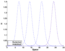
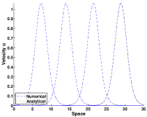
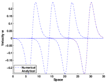
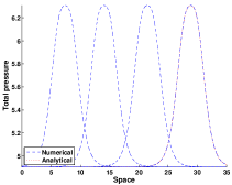
Figure 3. Propagation of the solitary wave at times $1.00008\,s,1.9009\,s,3.9017\,s$ and $5.9025\,s$. Comparison with analytical solution at time $t=5.9025\,s$.

In the projection step, the greatest difficulty is to compute the pressure corresponding to the boundary conditions of the hyperbolic part (as seen in 2.3). The solution near the boundary has been confronted to the analytical solution. In the following result, we set a Neumann boundary condition on the non hydrostatic pressure with the parameters given below. As shown in the figure 4, the pressure is well estimated at the outflow boundary and allows the wave to leave the domain with a good behavior.

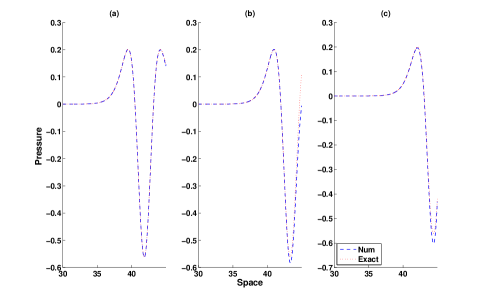
Figure 4. Non hydrostatic pressure profile at right boundary $(x=45\,m)$ (a): $t=9.4044\,s$ (b): $t=9.8046\,s$ (c): $t=10.1048\,s$.

The inflow boundary condition has been tested with this same test case and gives similar results. We are able to let the solitary wave enter in the domain with a good approximation of the elevation.

The numerical simulations for the first order method are compared with the analytical solution and the $L^{2}$- error has been evaluated over different meshes of sizes from 603 nodes to 6495 nodes (see figure 5). With the parameters given above, it gives a convergence rate close to $1$ for the two computations, i.e $\mathbb{P}_{1}$/$\mathbb{P}_{0}$ and $\mathbb{P}_{1}$-iso$\mathbb{P}_{2}$/$\mathbb{P}_{1}$.

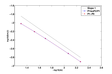
Figure 5. Convergence rate of the solitary wave solution for $\mathbb{P}_{1}$/$\mathbb{P}_{0}$ and $\mathbb{P}_{1}$-iso-$\mathbb{P}_{2}$/$\mathbb{P}_{1}$ scheme.

Notice that the parameters set to validate the method lead to have a significant non hydrostatic pressure (see the figure 4) and then, the results show the ability of the method to preserve the solitary wave over the time. The numerical results have also been obtained for the Thacker’s test presented in [1], with the same rate as the $\mathbb{P}_{1}$/$\mathbb{P}_{0}$ method.

5. Numerical results

5.1. Dam break problem

We next study the dispersive effect on the classical dam break problem, which is usually modeled by a Riemann problem providing a left state $(H_{L},u_{L})$ and a right state $(H_{R},u_{R})$ on each side of the discontinuity $x_{d}$ ([20]). However, our numerical dispersive model does not allow discontinuous solutions due to the variational spaces required for $H$ (see also [12]), thus we provide an initial data numerically close to the analytical one

$$H(x,0) = (H_{R}+a)-a\tanh\left(\frac{x-x_{d}}{\epsilon}\right),$$

$$a = H_{R}-H_{L}.$$

To evaluate the non hydrostatic effect, the different fields have been compared with the shallow water solution with the initial data: $H_{L}=1.8\,m$, $H_{R}=1\,m$, $u_{R}=u_{L}=0\,m.s^{-1}$, $\epsilon=10^{-4}\,m$, $x_{d}=300\,m$ over a domain of length $600\,m$ with $30000$ nodes. In figure 6, the evolution of the state is shown at time $t=10\,s$ and $t=45\,s$. The oscillations are due to the dispersive effects but the mean velocity does not change. These results are in adequation with the analysis proposed by Gavrilyuk in [28] for the Green-Naghdi model with the same configuration.

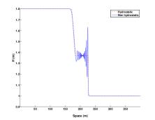
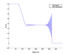
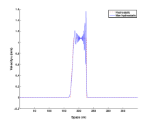
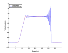
Figure 6. The dam break problem, elevation $H$ and velocity $u$ at times $t=10\,s$ and $t=45\,s$.

5.2. Wet-dry interfaces

The ability to treat the wet/dry interfaces is crucial in geophysical problems, since geophysicists are interested in studying the behavior of the water-depth near the shorelines. This implies a water depth tending to zero at such boundaries. To treat the problem, we use the method introduced in [1], considering a minimum elevation $H_{\epsilon}$.

Therefore, we confront the method with a coastal bottom at the right boundary over a domain of $35\,m$ with $3000$ nodes. A wave is generated at the left boundary with an amplitude of $0.2\,m$ and an initial water depth $H_{0}=1\,m$. In figure 7, the arrival of the wave at the coast is shown for times $t=7.91\,s$, $9.92\,s$ and $10.42\,s$.

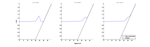
Figure 7. Propagation of a wave at a wet/dry interface.

5.3. Comparison with experimental results

In this part, we confront the model with Dingemans experiments (detailed in [18, 17]) that consist in generating a small amplitude wave at the left boundary of a channel with topography as described in figure 8.

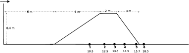
Figure 8. Configuration of Dingemans’s test.

At the left boundary, a wave is generated with a period $T=2.02\,s$ and an amplitude of $0.02\,m$. A free outflow condition is set at the right boundary. The initial free surface is set to be $\eta_{0}=0.4\,m$, and the measurement readings are saved at the following positions $10.5\,m$, $12.5\,m$, $13.5\,m$, $14.5\,m$ ,$15,7\,m$ and $17.3\,m$, placed at sensors $1$ to $6$ (fig.8 ). In such a situation, the non hydrostatic effects have a significant impact on the water depth that cannot be represented by a hydrostatic model. These effects result mainly from the slope of the bathymetry, $10\%$ in this case. In the figure 9, the simulation has been run with the hydrostatic model and the elevation has been compared with measures at the sensor $5$. As one can see, the non-hydrostatic pressure has to be taken in consideration to estimate the real water depth variation.

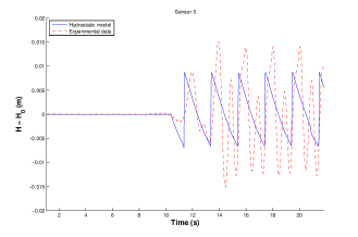
Figure 9. Comparison with hydrostatic model on sensor 5.

The numerical simulation with the non-hydrostatic model has been run with $15000$ nodes on a domain of $49\,m$ over $25\,s$ and the comparisons are illustrated for each sensor (fig. 10).

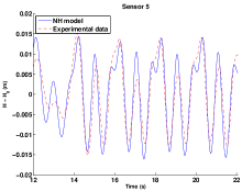
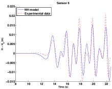
Figure 10. Comparison between measured and computed elevations on Dingemans test for the first six sensors.

The goal of this last result is also to highlight the ability of the model to capture dispersive effects for a geophysical flow with a non negligible pressure.

5.4. Remark on iterative method

We recall that this formulation should allow to extend the method on two dimensional unstructured grids. However, it requires to inverse a system at each time iteration, which will become too costly in two dimensions. To anticipate the two dimensional problem, this method has been tested using different iterative methods like conjugate gradient and Uzawa methods. In figure 11, we show a comparison of the computing time for the implementation $\mathbb{P}_{1}$-iso-$\mathbb{P}_{2}/\mathbb{P}_{1}$ and Uzawa method. In one dimension, it is not relevant to use one of these methods, while it will be necessary for the two dimension model.

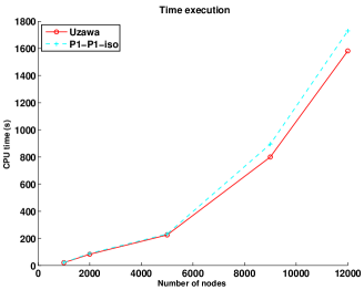
Figure 11. Comparison of the computing time (CPU) for the $\mathbb{P}_{1}$/$\mathbb{P}_{0}$ scheme, the $\mathbb{P}_{1}$-iso-$\mathbb{P}_{2}/\mathbb{P}_{1}$ and Uzawa method with $\mathbb{P}_{1}$-iso-$\mathbb{P}_{2}/\mathbb{P}_{1}$ solver with a tolerance $10^{-5}$.

6. Conclusion

In this paper, a variational formulation has been established for the one dimensional dispersive model introduced in [12]. The main idea is to give a new framework in which it will be possible to extend the scheme to the two dimensional model. To this aim, the finite-element method has been presented with two approximation spaces. First, the $\mathbb{P}_{1}$/$\mathbb{P}_{0}$ approximation has been done and we recover, as expected, the finite difference scheme, together with the good results proved in [1]. Then, the $\mathbb{P}_{1}$-iso-$\mathbb{P}_{2}$/$\mathbb{P}_{1}$approximation has been studied to prepare the two dimensional problem. We have validated the method using several numerical tests and studying the dispersive effect on geophysical situations.

References

- [1] N. Aïssiouene, M. O. Bristeau, E. Godlewski, and J. Sainte-Marie. A robust and stable numerical scheme for a depth-averaged Euler system. Submitted, pages –, 2015.
- [2] B. Alvarez-Samaniego and D. Lannes. Large time existence for 3D water-waves and asymptotics. Invent. Math., 171(3):485–541, 2008.
- [3] B. Alvarez-Samaniego and D. Lannes. A Nash-Moser theorem for singular evolution equations. Application to the Serre and Green-Naghdi equations. Indiana Univ. Math. J., 57(1):97–131, 2008.
- [4] E. Audusse, F. Bouchut, M.-O. Bristeau, R. Klein, and B. Perthame. A fast and stable well-balanced scheme with hydrostatic reconstruction for Shallow Water flows. SIAM J. Sci. Comput., 25(6):2050–2065, 2004.
- [5] E. Audusse, F. Bouchut, M.-O. Bristeau, and J. Sainte-Marie. Kinetic entropy inequality and hydrostatic reconstruction scheme for the Saint-Venant system. (Submitted) http://hal.inria.fr/hal-01063577/PDF/kin_hydrost.pdf, September 2014.
- [6] J.-L. Bona, T.-B. Benjamin, and J.-J. Mahony. Model equations for long waves in nonlinear dispersive systems. Philos. Trans. Royal Soc. London Series A, 272:47–78, 1972.
- [7] F. Bouchut. An introduction to finite volume methods for hyperbolic conservation laws. ESAIM Proc., 15:107–127, 2004.
- [8] F. Bouchut. Nonlinear stability of finite volume methods for hyperbolic conservation laws and well-balanced schemes for sources. Birkhäuser, 2004.
- [9] F. Brezzi. On the existence, uniqueness and approximation of saddle-point problems arising from Lagrangian multipliers. Rev. Française Automat. Informat. Recherche Opérationnelle Sér. Rouge, 8(R-2):129–151, 1974.
- [10] M-O. Bristeau and B. Coussin. Boundary Conditions for the Shallow Water Equations solved by Kinetic Schemes. Rapport de recherche RR-4282, INRIA, 2001. Projet M3N.
- [11] M.-O. Bristeau, N. Goutal, and J. Sainte-Marie. Numerical simulations of a non-hydrostatic Shallow Water model. Computers & Fluids, 47(1):51–64, 2011.
- [12] M. O. Bristeau, A. Mangeney, J. Sainte-Marie, and N. Seguin. An energy-consistent depth-averaged Euler system: derivation and properties. Discrete Contin. Dyn. Syst. Ser. B, 20(4):961–988, 2015.
- [13] M.-O. Bristeau and J. Sainte-Marie. Derivation of a non-hydrostatic shallow water model; Comparison with Saint-Venant and Boussinesq systems. Discrete Contin. Dyn. Syst. Ser. B, 10(4):733–759, 2008.
- [14] R. Camassa, D.D. Holm, and J.M. Hyman. A new integrable shallow water equation. Adv. Appl. Math., 31:23–40, 1993.
- [15] F. Chazel, D. Lannes, and F. Marche. Numerical simulation of strongly nonlinear and dispersive waves using a Green–Naghdi model. J. Sci. Comput., 48(1-3):105–116, July 2011.
- [16] A. J. Chorin. Numerical solution of the Navier-Stokes equations. Math. Comp., 22:745–762, 1968.
- [17] M.-W. Dingemans. Wave propagation over uneven bottoms. Advanced Series on Ocean Engineering - World Scientific, 1997.
- [18] M.W. Dingemans. Comparison of computations with boussinesq-like models and laboratory measurements. Technical Report H1684-12, AST G8M Coastal Morphodybamics Research Programme, 1994.
- [19] A. Duran and F. Marche. Discontinuous-Galerkin discretization of a new class of Green-Naghdi equations. Communications in Computational Physics, page 130, October 2014.
- [20] E. Godlewski and P.-A. Raviart. Numerical approximations of hyperbolic systems of conservation laws. Applied Mathematical Sciences, vol. 118, Springer, New York, 1996.
- [21] A.E. Green and P.M. Naghdi. A derivation of equations for wave propagation in water of variable depth. J. Fluid Mech., 78:237–246, 1976.
- [22] P.M. Gresho and S.T. Chan. Semi-consistent mass matrix techniques for solving the incompressible Navier-Stokes equations. First Int. Conf. on Comput. Methods in Flow Analysis, 1988. Okayama University, Japan.
- [23] J-L. Guermond. Some implementations of projection methods for Navier-Stokes equations. ESAIM: Mathematical Modelling and Numerical Analysis, 30(5):637–667, 1996.
- [24] J-L. Guermond and J. Shen. On the error estimates for the rotational pressure-correction projection methods. Math. Comput., 73(248):1719–1737, 2004.
- [25] Hans Johnston and Jian-Guo Liu. Accurate, stable and efficient Navier–Stokes solvers based on explicit treatment of the pressure term. Journal of Computational Physics, 199(1):221 – 259, 2004.
- [26] D. Lannes and P. Bonneton. Derivation of asymptotic two-dimensional time-dependent equations for surface water wave propagation. Physics of Fluids, 21(1):016601, 2009.
- [27] D. Lannes and F. Marche. A new class of fully nonlinear and weakly dispersive Green-Naghdi models for efficient 2D simulations. J. Comput. Phys., 282:238–268, 2015.
- [28] O. Le Métayer, S. Gavrilyuk, and S. Hank. A numerical scheme for the Green-Naghdi model. J. Comput. Phys., 229(6):2034–2045, 2010.
- [29] R.-J. LeVeque. Finite Volume Methods for Hyperbolic Problems. Cambridge University Press, 2002.
- [30] O. Nwogu. Alternative form of Boussinesq equations for nearshore wave propagation. Journal of Waterway, Port, Coastal and Ocean Engineering, ASCE, 119(6):618–638, 1993.
- [31] D.H. Peregrine. Long waves on a beach. J. Fluid Mech., 27:815–827, 1967.
- [32] O. Pironneau. Méthodes des éléments finis pour les fluides. Masson, 1988.
- [33] R. Rannacher. On Chorin’s projection method for the incompressible Navier-Stokes equations. In JohnG. Heywood, Kyûya Masuda, Reimund Rautmann, and VsevolodA. Solonnikov, editors, The Navier-Stokes Equations II — Theory and Numerical Methods, volume 1530 of Lecture Notes in Mathematics, pages 167–183. Springer Berlin Heidelberg, 1992.
- [34] J. Shen. Pseudo-compressibility methods for the unsteady incompressible Navier-Stokes equations. 11th AIAA Computational Fluid Dynamic Conference, 1993. Orlando, FL, USA.
- [35] J. Shen. On error estimates of the penalty method for unsteady Navier-Stokes equations. SIAM J. Numer. Anal., 32(2):386–403, 1995.