Fortran and C programs for the time-dependent dipolar Gross-Pitaevskii equation in an anisotropic trap

Abstract

Many of the static and dynamic properties of an atomic Bose-Einstein condensate (BEC) are usually studied by solving the mean-field Gross-Pitaevskii (GP) equation, which is a nonlinear partial differential equation for short-range atomic interaction. More recently, BEC of atoms with long-range dipolar atomic interaction are used in theoretical and experimental studies. For dipolar atomic interaction, the GP equation is a partial integro-differential equation, requiring complex algorithm for its numerical solution. Here we present numerical algorithms for both stationary and non-stationary solutions of the full three-dimensional (3D) GP equation for a dipolar BEC, including the contact interaction. We also consider the simplified one- (1D) and two-dimensional (2D) GP equations satisfied by cigar- and disk-shaped dipolar BECs. We employ the split-step Crank-Nicolson method with real- and imaginary-time propagations, respectively, for the numerical solution of the GP equation for dynamic and static properties of a dipolar BEC. The atoms are considered to be polarized along the $z$ axis and we consider ten different cases, e.g., stationary and non-stationary solutions of the GP equation for a dipolar BEC in 1D (along $x$ and $z$ axes), 2D (in $x-y$ and $x-z$ planes), and 3D, and we provide working codes in Fortran 90/95 and C for these ten cases (twenty programs in all). We present numerical results for energy, chemical potential, root-mean-square sizes and density of the dipolar BECs and, where available, compare them with results of other authors and of variational and Thomas-Fermi approximations.

Program summary

Program title: (i) imag1dZ, (ii) imag1dX, (iii) imag2dXY, (iv) imag2dXZ, (v) imag3d, (vi) real1dZ, (vii) real1dX, (viii) real2dXY, (ix) real2dXZ, (x) real3d

Catalogue identifier: AEWL_v1_0

Program summary URL: http://cpc.cs.qub.ac.uk/summaries/AEWL_v1_0.html

Program obtainable from: CPC Program Library, Queen’s University, Belfast, N. Ireland

Licensing provisions: Standard CPC licence, http://cpc.cs.qub.ac.uk/licence/licence.html

Distribution format: tar.gz

Programming language: Fortran 90/95 and C

Computer: Any modern computer with Fortran 90/95 or C language compiler installed.

Operating system: Linux, Unix

RAM: 1 GB (i,ii), 2 GB (iii,iv), 4 GB (v), 2 GB (vi,vii), 4 GB (viii,ix), 8 GB (x)

Classification: 2.9, 4.3, 4.12

Nature of problem: These programs are designed to solve the time-dependent nonlinear partial differential Gross-Pitaevskii (GP) equation with contact and dipolar interactions in one, two or three space dimensions in a harmonic anisotropic trap. The GP equation describes the properties of a dilute trapped Bose-Einstein condensate.

Solution method: The time-dependent GP equation is solved by the split-step Crank-Nicolson method by discretizing in space and time. The discretized equation is then solved by propagation, in either imaginary or real time, over small time steps. The contribution of the dipolar interaction is evaluated by a Fourier transformation (FT) to momentum space using a convolution theorem. The method yields the solution of stationary and/or non-stationary problems.

Additional comments: This package consists of 12 programs, see “Program title”, above. Fortran 90/95 and C versions are provided for each of the 6 programs. For the particular purpose of each program please see below.

Running time: Minutes on a medium PC (i, ii), tens of minutes on a medium PC (iii, iv), tens of minutes on a good workstation (v, vi).

1 Introduction

After the experimental realization of atomic Bose-Einstein condensate (BEC) of alkali-metal and some other atoms, there has been a great deal of theoretical activity in studying the statics and dynamics of the condensate using the mean-field time-dependent Gross-Pitaevskii (GP) equation under different trap symmetries [1]. The GP equation in three dimensions (3D) is a nonlinear partial differential equation in three space variables and a time variable and its numerical solution is indeed a difficult task specially for large nonlinearities encountered in realistic experimental situations [2]. Very special numerical algorithms are necessary for its precise numerical solution. In the case of alkali-metal atoms the atomic interaction in dilute BEC is essentially of short-range in nature and is approximated by a contact interaction and at zero tempearture is parametrized by a single parameter in a dilute BEC $-$ the s-wave atomic scattering length. Under this approximation the atomic interaction is represented by a cubic nonlinearity in the GP equation. Recently, we published the Fortran [3] and C [4] versions of useful programs for the numerical solution of the time-dependent GP equation with cubic nonlinearity under different trap symmetries using split-step Crank-Nicolson scheme and real- and imaginary-time propagations. Since then, these programs enjoyed widespread use [5].

More recently, there has been experimental observation of BEC of ⁵²Cr [6], ¹⁶⁴Dy [7] and ¹⁶⁸Er [8] atoms with large magnetic dipole moments. In this paper, for all trap symmetries the dipolar atoms are considered to be polarized along the $z$ axis. In these cases the atomic interaction has a long-range dipolar counterpart in addition to the usual contact interaction. The s-wave contact interaction is local and spherically symmetric, whereas the dipolar interaction acting in all partial waves is nonlocal and asymmetric. The resulting GP equation in this case is a partial integro-differential equation and special algorithms are required for its numerical solution. Different approaches to the numerical solution of the dipolar GP equation have been suggested [9, 10, 11, 12, 13, 14]. Yi and You [10] solve the dipolar GP equation for axially-symmetric trap while they perform the angular integral of the dipolar term, thus reducing it to one in axial ($z,z^{\prime}$) and radial ($\rho,\rho^{\prime}$) variables involving standard Elliptical integrals. The dipolar term is regularized by a cut-off at small distances and then evaluated numerically. The dipolar GP equation is then solved by imaginary-time propagation. Gòral and Santos [11] treat the dipolar term by a convolution theorem without approximation, thus transforming it to an inverse Fourier transformation (FT) of a product of the FT of the dipolar potential and the condensate density. The FT and inverse FT are then numerically evaluated by standard fast Fourier transformation (FFT) routines in Cartesian coordinates. The ground state of the system is obtained by employing a standard split-operator technique in imaginary time. This approach is used by some others [15]. Ronen et al. perform the angular integral in the dipolar term using axial symmetry. To evaluate it, in stead of FT in $x,y,$ and $z$ [11], they use Hankel transformation in the radial $\rho$ variable and FT in the axial $z$ variable. The ground state wave function is then obtained by imaginary-time propagation and dynamics by real-time propagation. This approach is also used by some others [16]. Bao et al. use Euler sine pseudospectral method for computing the ground states and a time-splitting sine pseudospectral method for computing the dynamics of dipolar BECs [9]. Blakie et al. solve the projected dipolar GP equation using a Hermite polynomial-based spectral representation [13]. Lahaye et al. use FT in $x,y,$ and $z$ to evaluate the dipolar term and employ imaginary- and real-time propagation after Crank-Nicolson discretization for stationary and nonstationary solution of the dipolar GP equation [14].

Here here we provide Fortran and C versions of programs for the solution of the dipolar GP equation in a fully anisotropic 3D trap by real- and imaginary-time propagation. We use split-step Crank-Nicolson scheme for the nondipolar part as in Refs. [3, 4] and the dipolar term is treated by FT in $x,y,z$ variables. We also present the Fortran and C programs for reduced dipolar GP equation in one (1D) and two dimensions (2D) appropriate for a cigar- and disk-shaped BEC under tight radial ($\rho$) and axial ($z$) trapping, respectively [17]. In the 1D case, we consider two possibilities: the 1D BEC could be aligned along the polarization direction $z$ or be aligned perpendicular to the polarization direction along $x$ axis. Similarly, in the 2D case, two possibilities are considered taking the 2D plane as $x-y$, perpendicular to polarization direction $z$ or as $x-z$ containing the polarization direction. This amounts to five different trapping possibilities $-$ two in 1D and 2D each and one in 3D $-$ and two solution schemes involving real- and imaginary-time propagation resulting in ten programs each in Fortran and C.

In Sec. 2 we present the 3D dipolar GP equation in an anisotropic trap. In addition to presenting the mean-field model and a general scheme for its numerical solution in Secs. 2.1 and 2.2, we also present two approximate solution schemes in Secs. 2.3 and 2.4, $-$ Gaussian variational approximation and Thomas-Fermi (TF) approximation $-$ in this case. The reduced 1D and 2D GP equations appropriate for a cigar- and a disk-shaped dipolar BEC are next presented in Secs. 2.5 and 2.6, respectively. The details about the computer programs, and their input/output files, etc. are given in Sec. 3. The numerical method and results are given in Sec. 4. Finally, a brief summary is given in Sec. 5.

2 Gross-Pitaevskii (GP) equation for dipolar condensates in three dimensions

2.1 The mean-field Gross-Pitaevskii equation

At ultra-low temperatures the properties of a dipolar condensate of $N_{\mathrm{at}}$ atoms, each of mass $m$, can be described by the mean-field GP equation with nonlocal nonlinearity of the form: [10, 18]

$$i\hbar\frac{\partial\phi({\mathbf{r}},t)}{\partial t}= \left[-\frac{\hbar^{2}}{2m}\nabla^{2}+V_{\text{trap}}({\mathbf{r}})+\frac{4\pi\hbar^{2}aN_{\mathrm{at}}}{m}\left|\phi({\mathbf{r}},t)\right|^{2}+N_{\mathrm{at}}\int U_{\mathrm{dd}}({\mathbf{r}}-{\mathbf{r}}^{\prime})\left|\phi({\mathbf{r}}^{\prime},t)\right|^{2}d{\mathbf{r}}^{\prime}\right]\phi({\mathbf{r}},t),$$ (1)

where $\int d{\bf r}|\phi({\mathbf{r}},t)|^{2}=1.$ The trapping potential, $V_{\text{trap}}$ is assumed to be fully asymmetric of the form

$$V_{\text{trap}}({\mathbf{r}})=\frac{1}{2}m\left(\omega_{x}^{2}x^{2}+\omega_{y}^{2}y^{2}+\omega_{z}^{2}z^{2}\right)$$

where $\omega_{x},\omega_{y}$ and $\omega_{z}$ are the trap frequencies, $a$ the atomic scattering length. The dipolar interaction, for magnetic dipoles, is given by [11, 16]

$$U_{\mathrm{dd}}(\bf R)=\frac{\mu_{0}\bar{\mu}^{2}}{4\pi}\frac{1-3\cos^{2}\theta}{|{\bf R}|^{3}},$$ (2)

where ${\bf R=r-r^{\prime}}$ determines the relative position of dipoles and $\theta$ is the angle between ${\bf R}$ and the direction of polarization $z$, $\mu_{0}$ is the permeability of free space and $\bar{\mu}$ is the dipole moment of the condensate atom. To compare the contact and dipolar interactions, often it is useful to introduce the length scale $a_{\mathrm{dd}}\equiv\mu_{0}\bar{\mu}^{2}m/(12\pi\hbar^{2})$ [6].

Convenient dimensionless parameters can be defined in terms of a reference frequency $\bar{\omega}$ and the corresponding oscillator length $l=\sqrt{\hbar/(m\bar{\omega})}$. Using dimensionless variables ${\bar{\bf r}}={\bf r}/l,{\bar{\bf R}}={\bf R}/l,\bar{a}=a/l,\bar{a}_{\mathrm{dd}}=a_{\mathrm{dd}}/l,\bar{t}=t\bar{\omega}$, $\bar{x}=x/l,\bar{y}=y/l,\bar{z}=z/l,\bar{\phi}=l^{3/2}\phi$, Eq. (1) can be rewritten (after removing the overhead bar from all the variables) as

$$i\frac{\partial\phi({\mathbf{r}},{t})}{\partial t} =\biggr{[}-\frac{1}{2}\nabla^{2}+\frac{1}{2}\left({\gamma^{2}x^{2}+\nu^{2}y^{2}}+\lambda^{2}z^{2}\right)+{4\pi aN_{\mathrm{at}}}|{\phi}|^{2}+3N_{\mathrm{at}}a_{\mathrm{dd}}\int V_{\mathrm{dd}}^{3D}({\bf{R}})|\phi({\mathbf{r}}^{\prime},t)|^{2}d{\mathbf{r}}^{\prime}\biggr{]}\phi({\mathbf{r}},{t}),$$ (3)

with

$$V_{\mathrm{dd}}^{3D}({\bf{R}})=\frac{1-3\cos^{2}\theta}{|{\bf{R}}|^{3}}\,,$$ (4)

where $\gamma=\omega_{x}/\bar{\omega},\nu=\omega_{y}/\bar{\omega},\lambda=\omega_{z}/\bar{\omega}$. The reference frequency $\bar{\omega}$ can be taken as one of the frequencies $\omega_{x},\omega_{y}$ or $\omega_{z}$ or their geometric mean $(\omega_{x}\omega_{y}\omega_{z})^{1/3}$. In the following we shall use Eq. (3) where we have removed the ‘bar’ from all variables.

Although we are mostly interested in the numerical solution of Eq. (3), in the following we describe two analytical approximation methods for its solution in the axially-symmetric case. These approximation methods $-$ the Gaussian variational and TF approximations $-$ provide reasonably accurate results under some limiting conditions and will be used for comparison with the numerical results. Also, we present reduced 1D and 2D mean-field GP equations appropriate for the description of a cigar and disk-shaped dipolar BEC under appropriate trapping condition. The numerical solution and variational approximation of these reduced equations will be discussed in this paper. A brief algebraic description of these topics are presented for the sake of completeness as appropriate for this study. For a full description of the same the reader is referred to the original publications.

2.2 Methodology

We perform numerical simulation of the 3D GP equation (3) using the split-step Crank-Nicolson method described in detail in Ref. [3]. Here we present the procedure to include the dipolar term in that algorithm. The inclusion of the dipolar integral term in the GP equation in coordinate space is not straightforward due to the singular behavior of the dipolar potential at short distances. It is interesting to note that this integral is well defined and finite. This problem has been tackled by evaluating the dipolar term in the momentum (k) space, where we do not face a singular behavior. The integral can be simplified in Fourier space by means of convolution as

$$\int d{\bf r}^{\prime}V_{\mathrm{dd}}^{3D}({\bf r}-{\bf r}^{\prime})n({\bf r^{\prime}},t)=\int\frac{d{\bf k}}{(2\pi)^{3}}e^{-i{\bf k\cdot r}}\widetilde{V}_{\mathrm{dd}}^{3D}({\bf k})\widetilde{n}({\bf k},t),$$ (5)

where $n({\bf r},t)=|\phi({\bf r},t)|^{2}$. The Fourier transformation (FT) and inverse FT, respectively, are defined by

$$\widetilde{A}({\bf k})=\int d{\bf r}A({\bf r})e^{i{\bf k}\cdot{\bf r}},\quad A({\bf r})=\frac{1}{(2\pi)^{3}}\int d{\bf k}\widetilde{A}({\bf k})e^{-i{\bf k}\cdot{\bf r}}.$$ (6)

The FT of the dipole potential can be obtained analytically [19]

$$\widetilde{V}_{\mathrm{dd}}^{3D}({\bf k})\equiv\frac{4\pi}{3}h_{3D}({\bf k})=\frac{4\pi}{3}\left(\frac{3k_{z}^{2}}{{\bf k}^{2}}-1\right),$$ (7)

so that

$$\int d{\bf r}^{\prime}V_{\mathrm{dd}}^{3D}({\bf r}-{\bf r}^{\prime})n({\bf r^{\prime}},t)=\frac{4\pi}{3}\int\frac{d{\bf k}}{(2\pi)^{3}}e^{-i{\bf k\cdot r}}h_{3D}({\bf k})\widetilde{n}({\bf k},t).$$ (8)

To obtain Eq. (7), first the angular integration is performed. Then a cut-off at small $r$ is introduced to perform the radial integration and eventually the zero cut-off limit is taken in the final result as shown in Appendix A of Ref. [19]. The FT of density $n({\bf r})$ is evaluated numerically by means of a standard FFT algorithm. The dipolar integral in Eq. (3) involving the FT of density multiplied by FT of dipolar interaction is evaluated by the convolution theorem (5). The inverse FT is taken by means of the standard FFT algorithm. The FFT algorithm is carried out in Cartesian coordinates and hence the GP equation is solved in 3D irrespective of the symmetry of the trapping potential. The dipolar interaction integrals in 1D and 2D GP equations are also evaluated in momentum spaces. The solution algorithm of the GP equation by the split-step Crank-Nicolson method is adopted from Refs. [3, 4].

The 3D GP equation (3) is numerically the most difficult to solve involving large RAM and CPU time. A requirement for the success of the split-step Crank-Nicolson method using a FT continuous at the origin is that on the boundary of the space discretization region the wave function and the interaction term should vanish. For the long-range dipolar potential this is not true and the FT (7) is discontinuous at the origin. The space domain (from $-\infty$ to $+\infty$) cannot be restricted to a small region in space just covering the spatial extention of the BEC as the same domain is also used to calculate the FT and inverse FT used in treating the long-range dipolar potential. The use and success of FFT implies a set of noninteracting 3D periodic lattice of BECs in different unit cells. This is not true for long-range dipolar interaction which will lead to an interaction between BECs in different cells. Thus, boundary effects can play a role when finding the FT. Hence a suffciently large space domain is to be used to have accurate values of the FT involving the long-range dipolar potential. It was suggested [12] that this could be avoided by truncating the dipolar interaction conveniently at large distances $r=R$ so that it does not affect the boundary, provided $R$ is taken to be larger than the size of the condensate. Then the truncated dipolar potential will cover the whole condensate wave function and will have a continuous FT at the origin. This will improve the accuracy of a calculation using a small space domain. The FT of the dipolar potential truncated at $r=R$, as suggested in Ref. [12], is used in the numerical routines

$$\widetilde{V}_{\mathrm{dd}}^{3D}({\bf k})=\frac{4\pi}{3}\left(\frac{3k_{z}^{2}}{{\bf k}^{2}}-1\right)\left[1+3\frac{\cos(kR)}{k^{2}R^{2}}-3\frac{\sin(kR)}{k^{3}R^{3}}\right],\quad\quad k=|{\bf k}|.$$ (9)

Needless to say, the diffculty in using a large space domain is the most severe in 3D. In 3D programs the cut-off $R$ of Eq. (9) improves the accuracy of calculation and a smaller space region can be used in numerical treatment. In 1D and 2D, a larger space domain can be used relatively easily and no cut-off has been used. Also, no convenient and effcient analytic cut-off is known in 1D and 2D [12]. The truncated dipolar potential (9) has only been used in the numerical programs in 3D, e.g., imag3d* and real3d*. In all other numerical programs in 1D and 2D, and in all analytic results reported in the following the untruncated potential (7) has been used.

2.3 Gaussian variational approximation

In the axially-symmetric case ($\gamma=\nu$), convenient analytic Lagrangian variational approximation of Eq. (3) can be obtained with the following Gaussian ansatz for the wave function [20]

$$\phi({\bf r},t)=\frac{\pi^{-3/4}}{w_{\rho}(t)\sqrt{w_{z}(t)}}\exp\left[-\frac{\rho^{2}}{2w_{\rho}^{2}(t)}-\frac{z^{2}}{2w_{z}^{2}(t)}+i\alpha(t)\rho^{2}+i\beta(t)z^{2}\right]$$ (10)

where ${\bf r}=\{\boldsymbol{\rho},z\},{\boldsymbol{\rho}}=\{x,y\}$, $w_{\rho}(t)$ and $w_{z}(t)$ are widths and $\alpha(t)$ and $\beta(t)$ are chirps. The time dependence of the variational parameters $w_{\rho}(t),$ $w_{z}(t)$, $\alpha(t)$ and $\beta(t)$ will not be explicitly shown in the following.

The Lagrangian density corresponding to Eq. (3) is given by

$${\cal L}({\bf r}) =\frac{i}{2}\left[\phi({\bf r})\frac{\phi^{*}({\bf r})}{\partial t}-\phi^{*}({\bf r})\frac{\partial\phi({\bf r})}{\partial t}\right]+\frac{|\nabla\phi({\bf r})|^{2}}{2}+\frac{1}{2}(\gamma^{2}\rho^{2}+\lambda^{2}z^{2})|\phi({\bf r})|^{2}+2\pi aN_{\mathrm{at}}|\phi({\bf r})|^{4}$$

$$+\frac{3a_{\mathrm{dd}}N_{\mathrm{at}}}{2}|\phi({\bf r})|^{2}\int V_{\mathrm{dd}}({\bf R})|\phi({\bf r^{\prime}})|^{2}d{\bf r^{\prime}}.$$ (11)

Consequently, the effective Lagrangian $L\equiv\int{\cal L}({\bf r})d{\bf r}$ (per particle) becomes [6, 21]

$$L=\omega_{\rho}^{2}\dot{\alpha}+\frac{\omega_{z}^{2}\dot{\beta}}{2}+\frac{\gamma^{2}\omega_{\rho}^{2}}{2}+\frac{\lambda^{2}\omega_{z}^{2}}{4}+\frac{1}{2\omega_{\rho}^{2}}+\frac{1}{4\omega_{z}^{2}}+2\omega_{\rho}^{2}\alpha^{2}+\omega_{z}^{2}\beta^{2}+\frac{N_{\mathrm{at}}[a-a_{\mathrm{dd}}f(\kappa)]}{\sqrt{2\pi}\omega_{\rho}^{2}\omega_{z}}.$$ (12)

The Euler-Lagrangian equations with this Lagrangian leads to the following set of coupled ordinary differential equations (ODE) for the widths $w_{\rho}$ and $w_{z}$ [22]

$$\ddot{w}_{\rho}+\gamma^{2}w_{\rho}=\frac{1}{w_{\rho}^{3}}+\frac{N_{\mathrm{at}}}{\sqrt{2\pi}}\frac{\left[2{a}-a_{\mathrm{dd}}{g(\kappa)}\right]}{w_{\rho}^{3}w_{z}},$$ (13)

$$\ddot{w}_{z}+\lambda^{2}w_{z}=\frac{1}{w_{z}^{3}}+\frac{2N_{\mathrm{at}}}{\sqrt{2\pi}}\frac{\left[{a}-a_{\mathrm{dd}}c(\kappa)\right]}{w_{\rho}^{2}w_{z}^{2}},$$ (14)

with $\kappa=w_{\rho}/w_{z}$ and

$$g(\kappa)=\frac{2-7\kappa^{2}-4\kappa^{4}+9\kappa^{4}d(\kappa)}{(1-\kappa^{2})^{2}},$$ (15)

$$c(\kappa)=\frac{1+10\kappa^{2}-2\kappa^{4}-9\kappa^{2}d(\kappa)}{(1-\kappa^{2})^{2}},$$ (16)

$$f(\kappa)=\frac{1+2\kappa^{2}-3\kappa^{2}d(\kappa)}{1-\kappa^{2}},\quad d(\kappa)=\frac{\mbox{atanh}\sqrt{1-\kappa^{2}}}{\sqrt{1-\kappa^{2}}}.$$ (17)

The widths of a (time-independent) stationary state are obtained from Eqs. (13) and (14) by setting $\ddot{w}_{\rho}=\ddot{w}_{z}=0$. The energy (per particle) of the stationary state is the Lagrangian (12) with $\alpha=\beta=0$, e.g.,

$$\frac{E}{N_{\mathrm{at}}}= \,\frac{1}{2w_{\rho}^{2}}+\frac{1}{4w_{z}^{2}}+\frac{N_{\mathrm{at}}[a-a_{\mathrm{dd}}f(\kappa)]}{\sqrt{2\pi}w_{z}w_{\rho}^{2}}+\frac{\gamma^{2}w_{\rho}^{2}}{2}+\frac{\lambda^{2}w_{z}^{2}}{4}.$$ (18)

The chemical potential $\mu=\partial E/\partial N_{\mathrm{at}}$ of the stationary state is given by [22]

$$\mu= \,\frac{1}{2w_{\rho}^{2}}+\frac{1}{4w_{z}^{2}}+\frac{2N_{\mathrm{at}}[a-a_{\mathrm{dd}}f(\kappa)]}{\sqrt{2\pi}w_{z}w_{\rho}^{2}}+\frac{\gamma^{2}w_{\rho}^{2}}{2}+\frac{\lambda^{2}w_{z}^{2}}{4}.$$ (19)

2.4 Thomas-Fermi (TF) approximation

In the time-dependent axially-symmetric GP equation (3), when the atomic interaction term is large compared to the kinetic energy gradient term, the kinetic energy can be neglected and the useful TF approximation emerges. We assume the normalized density of the dipolar BEC of the form [1, 23, 24, 25]

$$n({\mathbf{r}},t)\equiv|\phi({\bf r},t)|^{2}=\frac{15}{8\pi R_{\rho}^{2}(t)R_{z}(t)}\left[1-\frac{\rho^{2}}{R_{\rho}^{2}(t)}-\frac{z^{2}}{R_{z}^{2}(t)}\right],$$ (20)

where $R_{\rho}(t)$ and $R_{z}(t)$ are the radial and axial sizes. The time dependence of these sizes will not be explicitly shown in the following. Using the parabolic density (20), the energy functional $E_{TF}$ may be written as [24]

$$E_{TF}\equiv E_{\mathrm{trap}}+E_{\mathrm{int}}=\biggr{[}\frac{N(2\gamma^{2}R_{\rho}^{2}+\lambda^{2}R_{z}^{2})}{14}\biggr{]}+\biggr{[}\frac{15}{28\pi}\frac{4\pi aN_{\mathrm{at}}^{2}}{R_{\rho}^{2}R_{z}}\left\{1-\frac{a_{\mathrm{dd}}}{a}{f(\bar{\kappa})}\right\}\biggr{]},$$ (21)

where $\bar{\kappa}=R_{\rho}/R_{z}$ is the ratio of the condensate sizes and $f(\bar{\kappa})$ is given by Eq. (17). In Eq. (21), $E_{\mathrm{trap}}$ is the energy in the trap and $E_{\mathrm{int}}$ is the interaction or release energy in the TF approximation. In the TF regime one has the following set of coupled ODEs for the evolution of the condensate sizes [23]:

$$\ddot{R}_{\rho} =-{R_{\rho}}\gamma^{2}+\frac{15aN_{\mathrm{at}}}{R_{\rho}R_{z}}\left[\frac{1}{R_{\rho}^{2}}-\frac{a_{\mathrm{dd}}}{a}\left(\frac{1}{R_{\rho}^{2}}+\frac{3}{2}\frac{f(\bar{\kappa})}{R_{\rho}^{2}-R_{z}^{2}}\right)\right],$$ (22)

$$\ddot{R}_{z} =-\lambda^{2}R_{z}+\frac{15aN_{\mathrm{at}}}{R_{\rho}^{2}}\left[\frac{1}{R_{z}^{2}}+\frac{2a_{\mathrm{dd}}}{a}\left(\frac{1}{R_{z}^{2}}+\frac{3}{2}\frac{f(\bar{\kappa})}{R_{\rho}^{2}-R_{z}^{2}}\right)\right]..$$ (23)

The sizes of a stationary state can be calculated from Eqs. (22) and (23) by setting the time derivatives $\ddot{R}_{\rho}$ and $\ddot{R}_{z}$ to zero leading to the transcendental equation for $\bar{\kappa}$ [23]

$$3\bar{\kappa}^{2}\frac{a_{\mathrm{dd}}}{a}\left[\left(1+\frac{\lambda^{2}}{2\gamma^{2}}\right)\frac{f(\bar{\kappa})}{1-\bar{\kappa}^{2}}-1\right]+\left(\frac{a_{\mathrm{dd}}}{a}-1\right)\left(\bar{\kappa}^{2}-\frac{\lambda^{2}}{\gamma^{2}}\right)=0,$$ (24)

and

$$R_{\rho}=\left[\frac{15aN_{\mathrm{at}}\bar{\kappa}}{\gamma^{2}}\left\{1+\frac{a_{\mathrm{dd}}}{a}\left(\frac{3}{2}\frac{\bar{\kappa}^{2}f(\bar{\kappa})}{1-\bar{\kappa}^{2}}-1\right)\right\}\right]^{1/5},$$ (25)

with $R_{z}=R_{\rho}/\bar{\kappa}$. The chemical potential is given by [24]

$$\mu_{TF}\equiv E_{\mathrm{trap}}+2E_{\mathrm{int}}=\frac{15}{8\pi}\frac{4\pi aN_{\mathrm{at}}}{R_{\rho}^{2}R_{z}}\left[1-\frac{a_{\mathrm{dd}}}{a}f(\bar{\kappa})\right].$$ (26)

We have the identities $E_{TF}/N_{\mathrm{at}}=5\mu_{TF}/7,E_{\mathrm{int}}/N_{\mathrm{at}}=2\mu_{TF}/7,E_{\mathrm{trap}}/N_{\mathrm{at}}=3\mu_{TF}/7.$

2.5 One-dimensional GP equation for a cigar-shaped dipolar BEC

2.5.1 $z$ direction

For a cigar-shaped dipolar BEC with a strong axially-symmetric ($\nu=\gamma$) radial trap ($\lambda<\nu$, $\gamma$), we assume that the dynamics of the BEC in the radial direction is confined in the radial ground state [22, 26, 27]

$$\phi(\boldsymbol{\rho})=\exp(-\rho^{2}/2d_{\rho}^{2})/(d_{\rho}\sqrt{\pi}),\quad\gamma d_{\rho}^{2}=1,\quad\boldsymbol{\rho}\equiv(x,y),$$ (27)

of the transverse trap and the wave function $\phi({\bf r})$ can be written as

$$\phi({\bf r},t)\equiv\phi_{1D}(z,t)\times\phi(\boldsymbol{\rho})=\frac{1}{\sqrt{\pi d_{\rho}^{2}}}\exp\left[-\frac{\rho^{2}}{2d_{\rho}^{2}}\right]\phi_{1D}(z,t),$$ (28)

where $\phi_{1D}(z,t)$ is the effective 1D wave function for the axial dynamics and $d_{\rho}$ is the radial harmonic oscillator length.

To derive the effective 1D equation for the cigar-shaped dipolar BEC, we substitute the ansatz (28) in Eq. (3), multiply by the ground-state wave function $\phi(\boldsymbol{\rho})$ and integrate over $\boldsymbol{\rho}$ to get the 1D equation [22, 26]

$$i\frac{\partial\phi_{1D}(z,t)}{\partial t}=\left[-\frac{\partial_{z}^{2}}{2}+\frac{\lambda^{2}z^{2}}{2}+\frac{2aN_{\mathrm{at}}|\phi_{1D}|^{2}}{d_{\rho}^{2}}+{3a_{\mathrm{dd}}N_{\mathrm{at}}}\int_{-\infty}^{\infty}V^{1D}_{\mathrm{dd}}(|z-z^{\prime}|)|\phi_{1D}(z^{\prime},t)|^{2}dz^{\prime}\right]\phi_{1D}(z,t),$$ (29)

$$V_{\mathrm{dd}}^{1D}(Z)=\frac{2\pi}{\sqrt{2}d_{\rho}}\left[\frac{4}{3}\delta(\sqrt{w})+2\sqrt{w}-\sqrt{\pi}(1+2w)e^{w}\{1-\text{erf}(\sqrt{w})\}\right],$$ (30)

where $w=[Z/(\sqrt{2}d_{\rho})]^{2}$, $Z=|z-z^{\prime}|$. Here and in all reductions in Secs. 2.5 and 2.6 we use the untruncated dipolar potential (7) and not the truncated potential (9). The integral term in the 1D GP equation (29) is conveniently evaluated in momentum space using the following convolution identity [22]

$$\int_{-\infty}^{\infty}V^{1D}_{\mathrm{dd}}(|z-z^{\prime}|)|\phi_{1D}(z^{\prime},t)|^{2}dz^{\prime}=\frac{4\pi}{3}\int_{-\infty}^{\infty}\frac{dk_{z}}{2\pi}e^{-ik_{z}z}\widetilde{n}(k_{z},t)h_{1D}\left(\frac{k_{z}d_{\rho}}{\sqrt{2}}\right),$$ (31)

where

$$\widetilde{n}(k_{z},t)=\int_{-\infty}^{\infty}e^{ik_{z}z}|\phi_{1D}(z,t)|^{2}dz,$$ (32)

$$\widetilde{n}({\bf k}_{\rho})=\int e^{i{\bf k}_{\rho}\cdot\rho}|\phi_{2D}(\rho)|^{2}d\rho=e^{-k_{\rho}^{2}d_{\rho}^{2}/4},\quad k_{\rho}=\sqrt{k_{x}^{2}+k_{y}^{2}}$$ (33)

$$h_{1D}(\zeta)\equiv\frac{1}{(2\pi)^{2}}\int d{\bf k}_{\rho}\left[\frac{3k_{z}^{2}}{{\bf k}^{2}}-1\right]|\widetilde{n}({\bf k}_{\rho})|^{2}=\frac{1}{2\pi d_{\rho}^{2}}\int_{0}^{\infty}du\left[\frac{3\zeta^{2}}{u+\zeta^{2}}-1\right]e^{-u},\quad\zeta=\frac{k_{z}d_{\rho}}{\sqrt{2}}.$$ (34)

The 1D GP equation (29) can be solved analytically using the Lagrangian variational formalism with the following Gaussian ansatz for the wave function [22]:

$$\phi_{1D}(z,t)=\frac{\pi^{-1/4}}{\sqrt{w_{z}(t)}}\exp\left[-\frac{z^{2}}{2w_{z}^{2}(t)}+i\beta(t)z^{2}\right],$$ (35)

where $w_{z}(t)$ is the width and $\beta(t)$ is the chirp. The Lagrangian variational formalism leads to the following equation for the width $w_{z}(t)$ [22]:

$$\ddot{w}_{z}(t)+\lambda^{2}w_{z}(t)=\frac{1}{w_{z}^{3}(t)}+\frac{2N_{\mathrm{at}}}{\sqrt{2\pi}}\frac{\left[{a}-a_{\mathrm{dd}}c(\hat{\kappa})\right]}{d_{\rho}^{2}w_{z}^{2}(t)},\quad\hat{\kappa}=\frac{d_{\rho}}{w_{z}(t)}.$$ (36)

The time-independent width of a stationary state can be obtained from Eq. (36) by setting $\ddot{w}_{z}(t)=0$. The variational chemical potential for the stationary state is given by [22]

$$\mu=\frac{1}{4w_{z}^{2}}+\frac{2N_{\mathrm{at}}[a-a_{\mathrm{dd}}f(\hat{\kappa})]}{\sqrt{2\pi}w_{z}d_{\rho}^{2}}+\frac{\lambda^{2}w_{z}^{2}}{4}.$$ (37)

The energy per particle is given by

$$\frac{E}{N_{\mathrm{at}}}=\frac{1}{4w_{z}^{2}}+\frac{N_{\mathrm{at}}[a-a_{\mathrm{dd}}f(\hat{\kappa})]}{\sqrt{2\pi}w_{z}d_{\rho}^{2}}+\frac{\lambda^{2}w_{z}^{2}}{4}.$$ (38)

2.5.2 $x$ direction

For a cigar-shaped dipolar BEC with a strong axially-symmetric ($\nu=\lambda$) radial trap ($\gamma<\nu$, $\lambda$), we assume that the dynamics of the BEC in the radial direction is confined in the radial ground state [22, 26, 27]

$$\phi(\boldsymbol{\rho})=\exp(-\rho^{2}/2d_{\rho}^{2})/(d_{\rho}\sqrt{\pi}),\quad\nu d_{\rho}^{2}=1,\quad\boldsymbol{\rho}\equiv(y,z),$$ (39)

of the transverse trap and the wave function $\phi({\bf r})$ can be written as

$$\phi({\bf r},t)\equiv\phi_{1D}(x,t)\times\phi(\boldsymbol{\rho})=\frac{1}{\sqrt{\pi d_{\rho}^{2}}}\exp\left[-\frac{\rho^{2}}{2d_{\rho}^{2}}\right]\phi_{1D}(x,t),$$ (40)

where $\phi_{1D}(x,t)$ is the effective 1D wave function for the dynamics along $x$ axis and $d_{\rho}$ is the radial harmonic oscillator length.

To derive the effective 1D equation for the cigar-shaped dipolar BEC, we substitute the ansatz (40) in Eq. (3), multiply by the ground-state wave function $\phi(\boldsymbol{\rho})$ and integrate over $\boldsymbol{\rho}$ to get the 1D equation

$$i\frac{\partial\phi_{1D}(x,t)}{\partial t}=\left[-\frac{\partial_{x}^{2}}{2}+\frac{\gamma^{2}x^{2}}{2}+\frac{2aN_{\mathrm{at}}|\phi_{1D}|^{2}}{d_{\rho}^{2}}+{4\pi a_{\mathrm{dd}}N_{\mathrm{at}}}\int_{-\infty}^{\infty}\frac{dk_{x}}{2\pi}e^{-ik_{x}x}\widetilde{n}(k_{x},t)j_{1D}(\tau_{x})\right]\phi_{1D}(x,t),$$ (41)

where $\tau_{x}=d_{\rho}k_{x}/\sqrt{2}$ and

$$j_{1D}(\tau_{x})\equiv\frac{1}{(2\pi)^{2}}\int d{\bf k}_{\rho}\left[\frac{3k_{z}^{2}}{{\bf k}^{2}}-1\right]|\widetilde{n}({\bf k}_{\rho})|^{2}=\frac{\sqrt{2}}{2\pi d_{\rho}}\int_{-\infty}^{\infty}d\tau_{y}e^{-\tau_{y}^{2}}h_{2D}(\tau),\quad\tau_{y}=\frac{d_{\rho}k_{y}}{\sqrt{2}},\quad\tau=\sqrt{\tau_{x}^{2}+\tau_{y}^{2}},$$ (42)

$$h_{2D}(\tau)=\frac{1}{\sqrt{2\pi}d_{\rho}}[2-3\sqrt{\pi}e^{\tau^{2}}\tau\{1-\text{erf}(\tau)\}].$$ (43)

To derive Eq. (41), the dipolar term in Eq. (3) is first written in momentum space using Eq. (8) and the integrations over $k_{y}$ and $k_{z}$ are performed in the dipolar term.

2.6 Two-dimensional GP equation for a disk-shaped dipolar BEC

2.6.1 $x-y$ plane

For an axially-symmetric ($\nu=\gamma$) disk-shaped dipolar BEC with a strong axial trap ($\lambda>\nu$, $\gamma$), we assume that the dynamics of the BEC in the axial direction is confined in the axial ground state

$$\phi(z)=\exp(-z^{2}/2d_{z}^{2})/(\pi d_{z}^{2})^{1/4},\quad d_{z}=\sqrt{1/(\lambda)},$$ (44)

and we have for the wave function

$$\phi({\bf r})\equiv\phi(z)\times\phi_{2D}(\boldsymbol{\rho},t)=\frac{1}{(\pi d_{z}^{2})^{1/4}}\exp\left[-\frac{z^{2}}{2d_{z}^{2}}\right]\phi_{2D}(\boldsymbol{\rho},t),$$ (45)

where $\boldsymbol{\rho}\equiv(x,y)$, $\phi_{2D}(\boldsymbol{\rho},t)$ is the effective 2D wave function for the radial dynamics and $d_{z}$ is the axial harmonic oscillator length. To derive the effective 2D equation for the disk-shaped dipolar BEC, we use ansatz (45) in Eq. (3), multiply by the ground-state wave function $\phi(z)$ and integrate over $z$ to get the 2D equation [22, 28]

$$i\frac{\partial\phi_{2D}(\boldsymbol{\rho},t)}{\partial t}=\left[-\frac{\nabla_{\rho}^{2}}{2}+\frac{\gamma^{2}x^{2}+\nu^{2}y^{2}}{2}+\frac{4\pi aN_{\mathrm{at}}|\phi_{2D}|^{2}}{\sqrt{2\pi}d_{z}}+{4\pi}a_{\mathrm{dd}}N_{\mathrm{at}}\int\frac{d{\bf k}_{\rho}}{(2\pi)^{2}}e^{-i{\bf k}_{\rho}.\boldsymbol{\rho}}\widetilde{n}({\bf k}_{\rho},t)h_{2D}\biggr{(}\frac{k_{\rho}d_{z}}{\sqrt{2}}\biggr{)}\right]\phi_{2D}(\boldsymbol{\rho},t),$$ (46)

where $k_{\rho}=\sqrt{k_{x}^{2}+k_{y}^{2}}$, and

$$\widetilde{n}({\bf k}_{\rho},t)=\int d\boldsymbol{\rho}e^{i{\bf k}_{\rho}.\boldsymbol{\rho}}|\phi_{2D}(\boldsymbol{\rho},t)|^{2},\quad\widetilde{n}(k_{z})=\int dze^{ik_{z}z}|\phi(z)|^{2}=e^{-k_{z}^{2}d_{z}^{2}/4,}$$ (47)

$$h_{2D}(\xi)\equiv\frac{1}{2\pi}\int^{\infty}_{-\infty}dk_{z}\left[\frac{3k_{z}^{2}}{{\bf k}^{2}}-1\right]|\widetilde{n}(k_{z})|^{2}=\frac{1}{\sqrt{2\pi}d_{z}}[2-3\sqrt{\pi}\xi\exp(\xi^{2})\{1-\text{erf}(\xi)\}],\quad\xi=\frac{k_{\rho}d_{z}}{\sqrt{2}}.$$ (48)

To derive Eq. (46), the dipolar term in Eq. (3) is first written in momentum space using Eq. (8) and the integration over $k_{z}$ is performed in the dipolar term.

The 2D GP equation (46) can be solved analytically using the Lagrangian variational formalism with the following Gaussian ansatz for the wave function [22]:

$$\phi_{2D}(\boldsymbol{\rho},t)=\frac{\pi^{-1/2}}{w_{\rho}(t)}\exp\left[-\frac{\rho^{2}}{2w_{\rho}^{2}(t)}+i\alpha(t)\rho^{2}\right],$$ (49)

where $w_{\rho}(t)$ is the width and $\alpha(t)$ is the chirp. The Lagrangian variational formalism leads to the following equation for the width $w_{\rho}$ [22]:

$$\ddot{w}_{\rho}(t)+\gamma^{2}w_{\rho}(t)=\frac{1}{w_{\rho}^{3}(t)}+\frac{N_{\mathrm{at}}}{\sqrt{2\pi}}\frac{\left[2a-a_{\mathrm{dd}}g(\bar{\kappa})\right]}{w_{\rho}^{3}(t)d_{z}},\quad\bar{\kappa}=\frac{w_{\rho}(t)}{d_{z}}.$$ (50)

The time-independent width of a stationary state can be obtained from Eq. (50) by setting $\ddot{w}_{\rho}(t)=0$. The variational chemical potential for the stationary state is given by [22]

$$\mu=\frac{1}{2w_{\rho}^{2}}+\frac{2N_{\mathrm{at}}[a-a_{\mathrm{dd}}f(\bar{\kappa})]}{\sqrt{2\pi}d_{z}w_{\rho}^{2}}+\frac{\gamma^{2}w_{\rho}^{2}}{2}.$$ (51)

The energy per particle is given by

$$\frac{E}{N_{\mathrm{at}}}=\frac{1}{2w_{\rho}^{2}}+\frac{N_{\mathrm{at}}[a-a_{\mathrm{dd}}f(\bar{\kappa})]}{\sqrt{2\pi}d_{z}w_{\rho}^{2}}+\frac{\gamma^{2}w_{\rho}^{2}}{2}.$$ (52)

2.6.2 $x-z$ plane

For a disk-shaped dipolar BEC with a strong axial trap along $y$ direction ($\nu>\lambda$, $\gamma$), we assume that the dynamics of the BEC in the $y$ direction is confined in the ground state

$$\phi(y)=\exp(-y^{2}/2d_{y}^{2})/(\pi d_{y}^{2})^{1/4},\quad d_{y}=\sqrt{1/(\nu)},$$ (53)

and we have for the wave function

$$\phi({\bf r})\equiv\phi(y)\times\phi_{2D}(\boldsymbol{\rho}{},t)=\frac{1}{(\pi d_{y}^{2})^{1/4}}\exp\left[-\frac{y^{2}}{2d_{y}^{2}}\right]\phi_{2D}(\boldsymbol{\rho}{},t),$$ (54)

where now $\boldsymbol{\rho}{}\equiv(x,z)$, and $\phi_{2D}(\boldsymbol{\rho}{},t)$ is the circularly-asymmetric effective 2D wave function for the 2D dynamics and $d_{y}$ is the harmonic oscillator length along $y$ direction. To derive the effective 2D equation for the disk-shaped dipolar BEC, we use ansatz (54) in Eq. (3), multiply by the ground-state wave function $\phi(y)$ and integrate over $y$ to get the 2D equation

$$i\frac{\partial\phi_{2D}(\boldsymbol{\rho},t)}{\partial t}=\left[-\frac{\nabla_{\rho}^{2}}{2}+\frac{\gamma^{2}x^{2}+\lambda^{2}z^{2}}{2}+\frac{4\pi aN_{\mathrm{at}}|\phi_{2D}|^{2}}{\sqrt{2\pi}d_{y}}+{4\pi a_{\mathrm{dd}}N_{\mathrm{at}}}\int\frac{d{\bf k}_{\rho}}{(2\pi)^{2}}e^{-i{\bf k}_{\rho}.\boldsymbol{\rho}}\widetilde{n}({\bf k}_{\rho},t)j_{2D}\biggr{(}\frac{k_{\rho}d_{y}}{\sqrt{2}}\biggr{)}\right]\phi_{2D}(\boldsymbol{\rho},t),$$ (55)

where $k_{\rho}=\sqrt{k_{z}^{2}+k_{x}^{2}}$, and

$$j_{2D}(\xi)\equiv\frac{1}{2\pi}\int^{\infty}_{-\infty}dk_{y}\left[\frac{3k_{z}^{2}}{{\bf k}^{2}}-1\right]|\widetilde{n}(k_{y})|^{2}=\frac{1}{\sqrt{2\pi}d_{y}}[-1+3\sqrt{\pi}\frac{\xi_{z}^{2}}{\xi}\exp(\xi^{2})\{1-\text{erf}(\xi)\}],\quad\xi=\frac{k_{\rho}d_{y}}{\sqrt{2}},\xi_{z}=\frac{k_{z}d_{y}}{\sqrt{2}}.$$ (56)

To derive Eq. (55), the dipolar term in Eq. (3) is first written in momentum space using Eq. (8) and the integration over $k_{y}$ is performed in the dipolar term.

3 Details about the programs

3.1 Description of the programs

In this subsection we describe the numerical codes for solving the dipolar GP equations (29) and (41) in 1D, Eq. (46) and (55) in 2D, and Eq. (3) in 3D using real- and imaginary-time propagations. The real-time propagation yields the time-dependent dynamical results and the imaginary-time propagation yields the time-independent stationary solution for the lowest-energy state for a specific symmetry. We use the split-step Crank-Nicolson method for the solution of the equations described in Ref. [3]. The present programs have the same structure as in Ref. [3] with added subroutines to calculate the dipolar integrals. In the absence of dipolar interaction the present programs will be identical with the previously published ones [3]. A general instruction to use these programs in the nondipolar case can be found in Ref. [3] and we refer the interested reader to this article for the same.

The present Fortran programs named (‘imag1dX.f90’, ‘imag1dZ.f90’), (‘imag2dXY.f90’, ‘imag2dXZ.f90’), ‘imag3d.f90’, (‘real1dX.f90’, ‘real1dZ.f90’), (‘real2dXY.f90’, ‘real2dXZ.f90’), ‘real3d.f90’, deal with imaginary- and real-time propagations in 1D, 2D, and 3D and are to be contrasted with previously published programs [3] ‘imagtime1d.F’, ‘imagtime2d.f90’, ‘imagtime3d.f90’, ‘realtime1d.F’, ‘realtime2d.f90’, and ‘realtime3d.f90’, for the nondipolar case. The input parameters in Fortran programs are introduced in the beginning of each program. The corresponding C codes are called (imag1dX.c, imag1dX.h, imag1dZ.c, imag1dZ.h,), (imag2dXY.c, imag2dXY.h, imag2dXZ.c, imag2dXZ.h,), (imag3d.c, imag3d.h), (real1dX.c, real1dX.h, real1dZ.c, real1dZ.h,), (real2dXY.c, real2dXY.h, real2dXZ.c, real2dXZ.h,), (real3d.c, real3d.h), with respective input files (‘imag1dX-input’, ‘imag1dZ-input’), (‘imag2dXY-input’, ‘imag2dXZ-input’), ‘imag3d-input’, (‘real1dX-input’,‘real1dZ-input’), (‘real2dXY-input’, ‘real1dXZ-input’), ‘real3d-input’, which perform identical executions as in the Fortran programs.

We present in the following a description of input parameters. The parameters NX, NY, and NZ in 3D (NX and NY in 2DXY, NX and NZ in 2DXZ), and N in 1D stand for total number of space points in $x$, $y$ and $z$ directions, where the respective space steps DX, DY, and DZ can be made equal or different; DT is the time step. The parameters NSTP, NPAS, and NRUN denote number of time iterations. The parameters GAMMA ($\gamma$), NU ($\nu$), and LAMBDA ($\lambda$) denote the anisotropy of the trap. The number of atoms is denoted NATOMS ($N_{\mathrm{at}}$), the scattering length is denoted AS ($a$) and dipolar length ADD ($a_{\mathrm{dd}}$). The parameters G0 ($4\pi N_{\mathrm{at}}a$) and GDD0 ($3a_{\mathrm{dd}}N_{\mathrm{at}}$) are the contact and dipolar nonlinearities. The parameter OPTION = 2 (default) defines the equations of the present paper with a factor of half before the kinetic energy and trap; OPTION = 1 defines a different set of GP equations without these factors, viz Ref. [3]. The parameter AHO is the unit of length and Bohr_a0 is the Bohr radius. In 1D the parameter DRHO is the radial harmonic oscillator $d_{\rho}$ and in 2D the parameter D$\_$Z or D$\_$Y is the axial harmonic oscillator length $d_{z}$ or $d_{y}$. The parameter CUTOFF is the cut-off $R$ of Eq. (9) in the 3D programs. The parameters GPAR and GDPAR are constants which multiply the nonlinearities G0 and GDD0 in realtime routines before NRUN time iterations to study the dynamics.

The programs, as supplied, solve the GP equations for specific values of dipolar and contact nonlinearities and write the wave function, chemical potential, energy, and root-mean-square (rms) size(s) etc. For solving a stationary problem, the imaginary-time programs are far more accurate and should be used. The real-time programs should be used for studying non-equilibrium problems reading an initial wave function calculated by the imaginary-time program with identical set of parameters (set NSTP = 0, for this purpose, in the real-time programs). The real-time programs can also calculate stationary solutions in NSTP time steps (set NSTP $\neq$ 0 in real-time programs), however, with less accuracy compared to the imaginary-time programs. The larger the value of NSTP in real-time programs, more accurate will be the result [3]. The nonzero integer parameter NSTP refers to the number of time iterations during which the nonlinear terms are slowly introduced during the time propagation for calculating the wave function. After introducing the nonlinearities in NSTP iterations the imaginary-time programs calculate the final result in NPAS plus NRUN time steps and write some of the results after NPAS steps to check convergence. The real-time programs run the dynamics during NPAS steps with unchanged initial parameters so as to check the stability and accuracy of the results. Some of the nonlinearities are then slightly modified after NPAS iterations and the small oscillation of the system is studied during NRUN iterations.

Each program is preset at fixed values of contact and dipolar nonlinearities as calculated from input scattering length(s), dipolar strength(s), and number of atom(s), correlated DX-DT values and NSTP, NPAS, and NRUN, etc. A study of the correlated DX and DT values in the nondipolar case can be found in Ref. [3]. Smaller the steps DX, DY, DZ and DT, more accurate will be the result, provided we integrate over a reasonably large space region by increasing NX, NY, and NZ, etc. Each supplied program produces result up to a desired precision consistent with the parameters employed $-$ G0, GDD0, DX, DY, DZ, DT, NX, NY, NZ, NSTP, NPAS, and NRUN etc.

3.2 Description of Output files

Programs ‘imag$n$d*’ ($n=1,2,3,$ C and Fortran): They write final density in files ‘imag$n$d-den.txt’ after NRUN iterations. In addition, in 2D and 3D, integrated 1D densities ‘imag$n$d*-den1d_x.txt’, ‘imag$n$d*-den1d_y.txt’,‘imag$n$d*-den1d_z.txt’, along x, y, and z, etc, are given. These densities are obtained by integrating the densities over eliminated space variables. In addition, in 3D integrated 2D densities ‘imag3d-den2d_xy.txt’, ‘imag3d-den2d_yz.txt’,‘imag3d-den2d_zx.txt’, in xy, yz, and zx planes can be written (commented out by default). The files ‘imag$n$d*-out.txt’ provide different initial input data, as well as chemical potential, energy, size, etc at different stages (initial, after NSTP, NPAS, and after NRUN iterations), from which a convergence of the result can be inferred. The files ‘imag$n$d*-rms.txt’ provide the different rms sizes at different stages (initial, after NSTP, NPAS, and after NRUN iterations).

Programs ‘real$n$d*’ ($n=1,2,3,$ C and Fortran): The same output files as in the imaginary-time programs are available in the real-time programs. The real-time densities are reported after NPAS iterations. In addition in the ‘real$n$d*-dyna.txt’ file the temporal evolution of the widths are given during NPAS and NRUN iterations. Before NRUN iterations the nonlinearities G0 and GDD0 are multiplied by parameters GPAR and GDPAR to start an oscillation dynamics.

3.3 Running the programs

In addition to installing the respective Fortran and C compilers one needs also to install the FFT routine FFTW in the computer. To run the Fortran programs the supplied routine fftw3.f03 should be included in compilation. The commands for running the Fortran programs using INTEL, GFortran, and Oracle Sun compilers are given inside the Fortran programs. The programs are submitted in directories with option to compile using the command ‘make’. There are two files with general information about the programs and FT for user named ’readme.txt’ and ‘readme-fftw.txt’. The Fortran and C programs are in directories ../f$\_$program and ../c$\_$program. Inside these directories there are subdirectories such as ../input, ../output, ../src. The subdirectory ../output contains output files the programs generate, ../input contains input files for C programs, and ../src contains the different programs. The command ‘make’ in the directory ../f$\_$program or ../c$\_$program compiles all the programs and generates the corresponding executable files to run. The command ‘make’ for INTEL, GFortran and OracleSun Fortran are given.

4 Numerical Results

In this section we present results for energy, chemical potential and root-mean-square (rms) sizes for different stationary BECs in 1D, 2D, and 3D, and compare with those obtained by using Gaussian variational and TF approximations, wherever possible. We also compare with available results by other authors. For a fixed space and time step, sufficient number of space discretizing points and time iterations are to be allowed to get convergence.

Table 1: The energy per particle $E/N_{\mathrm{at}}$, chemical potential $\mu$, and rms size $\langle z\rangle$ of the 1D GP equation (29) for $\lambda=1,d_{\rho}=1$ $\mu$m for the ⁵²Cr BEC with $a=6$ nm, $a_{\mathrm{dd}}=16a_{0}$ and different number of atoms $N_{\mathrm{at}}$. In Eqs. (3) and (29) the lengths are expressed in oscillator unit: $l=1$ $\mu$m. Numerical results are calculated for parameters (A) $dz=0.05,dt=0.0005,N=2048$ (B) $dz=0.1,dt=0.001,N=1024$ and compared with variational results obtained from Eqs. (36), (37) and (38).

$N_{\mathrm{at}}$	$\langle z\rangle$	$\langle z\rangle$	$\langle z\rangle$	$E/N_{\mathrm{at}}$	$E/N_{\mathrm{at}}$	$E/N_{\mathrm{at}}$	$\mu$	$\mu$	$\mu$
	var	(B)	(A)	var	(B)	(A)	var	(B)	(A)
100	0.7939	0.7937	0.7937	0.7239	0.7222	0.7222	0.9344	0.9297	0.9297
500	1.0425	1.0381	1.0381	1.4371	1.4166	1.4166	2.2157	2.1691	2.1691
1000	1.2477	1.2375	1.2375	2.1376	2.0920	2.0920	3.4165	3.3234	3.3234
5000	2.0249	1.9939	1.9939	5.8739	5.6910	5.6910	9.6671	9.3488	9.3488
10000	2.5233	2.4815	2.4815	9.2129	8.913	8.913	15.223	14.715	14.715
50000	4.2451	4.1719	4.1719	26.505	25.622	25.622	43.993	42.527	42.527

First we present in table 1 numerical results for the energy $E$, chemical potential $\mu$, and rms size $\langle z\rangle$ calculated using the imaginary-time program for the 1D dipolar GP equation (29) for ⁵²Cr atoms with $a=6$ nm ($\approx 113a_{0}$ with $a_{0}$ the Bohr radius), and $a_{\mathrm{dd}}=16a_{0}$ for $\lambda=1,d_{\rho}=1,l=1$ $\mu$m and for different number of atoms $N_{\mathrm{at}}$ and different space and time steps $dz$ and $dt$. The Gaussian variational approximations obtained from Eqs. (36), (37) and (38) are also given for comparison. The variational results provide better approximation to the numerical solution for a smaller number of atoms.

Table 2: The energy per particle $E/N_{\mathrm{at}}$, chemical potential $\mu$, and rms size $\langle\rho\rangle$ of the 2D GP equation (46) for $\gamma=\nu=1,d_{z}=1$ $\mu$m for the ⁵²Cr BEC with $a=6$ nm, $a_{\mathrm{dd}}=16a_{0}$ and different number of atoms $N_{\mathrm{at}}$. In Eqs. (3) and (46) the lengths are expressed in oscillator unit: $l=1$ $\mu$m. Numerical results are calculated for space and time steps (A) $dx=dy=0.1,dt=0.0005,NX=NY\equiv{\cal N}=768,$ (B) $dx=dy=0.2,dt=0.002,{\cal N}=384,$ and compared with variational results obtained from Eqs. (50), (51) and (52).

$N_{\mathrm{at}}$	$\langle\rho\rangle$	$\langle\rho\rangle$	$\langle\rho\rangle$	$E/N_{\mathrm{at}}$	$E/N_{\mathrm{at}}$	$E/N_{\mathrm{at}}$	$\mu$	$\mu$	$\mu$
	var	(B)	(A)	var	(B)	(A)	var	(B)	(A)
100	1.0985	1.097	1.097	1.2182	1.2156	1.2157	1.4187	1.4120	1.4119
500	1.3514	1.342	1.342	1.8653	1.8383	1.8383	2.5437	2.4840	2.4840
1000	1.5482	1.530	1.531	2.4571	2.3988	2.3988	3.5070	3.3901	3.3901
5000	2.2549	2.208	2.208	5.2206	4.9989	4.9989	7.8005	7.4249	7.4249
10000	2.6824	2.619	2.619	7.3787	7.029	7.029	11.090	10.522	10.522
50000	4.0420	3.934	3.934	16.680	15.793	15.793	25.161	23.789	23.789

In table 2 we present results for the energy $E$, chemical potential $\mu$, and rms size $\langle\rho\rangle$ of the 2D GP equation (46) for $\gamma=\nu=1,d_{z}=1,l=1$ $\mu$m. The numerical results are calculated using different space and time steps $dx,dy$ and $dt$ and different number $N_{\mathrm{at}}$ of ⁵²Cr atoms with $a_{\mathrm{dd}}=16a_{0}$ and $a=6$ nm. Axially-symmetric Gaussian variational approximations obtained from Eqs. (50), (51) and (52) are also presented for comparison.

Table 3: Energy per particle $E/N_{\mathrm{at}}$ and chemical potential $\mu$ from a solution of Eq. (3) for $\gamma=\nu=1,\lambda^{2}=0.25,a=0$ and different nonlinearity $g_{\mathrm{dd}}\equiv 3a_{\mathrm{dd}}N_{\mathrm{at}}$. The present numerical results are compared with Gaussian variational results obtained from Eqs. (18) and (19) as well as numerical results of Asad-uz-Zaman et al. [16, 29]. Numerical results are calculated for the following space and time steps and the following space discretizing points in the Crank-Nicolson discretization: (A) $dx=dy=dz=0.05,dt=0.0004,$ $(NX=NY=NZ\equiv{\cal N}=384)$; (B) $0.1,dt=0.002,$ $({\cal N}=128,R=6)$; and (C) $0.2,dt=0.007,$ $({\cal N}=64,R=6)$.

$g_{\mathrm{dd}}$	$E/N_{\mathrm{at}}$	$E/N_{\mathrm{at}}$	$E/N_{\mathrm{at}}$	$E/N_{\mathrm{at}}$	$E/N_{\mathrm{at}}$	$\mu$	$\mu$	$\mu$	$\mu$	$\mu$
	var	(C)	(B)	(A)	[29]	var	(C)	(B)	(A)	[29]
0	1.2500	1.2498	1.2500	1.2500	1.2500	1.2500	1.2498	1.2500	1.2500	1.2500
1	1.2230	1.2220	1.2222	1.2222	1.2222	1.1934	1.1910	1.1912	1.1911	1.1911
2	1.1907	1.1872	1.1875	1.1874	1.1874	1.1203	1.1100	1.1100	1.1100	1.1100
3	1.1521	1.143	1.1439	1.1438	1.1437	1.0253	0.995	0.996	0.996	0.9955
4	1.1051	1.085	1.0857	1.0857	1.0856	0.8950	0.805	0.803	0.806	0.8062

Now we present results of the solution of the 3D GP equation (3) with some axially-symmetric traps. In this case we take advantage of the cut-off introduced in Eq. (9) to improve the accuracy of the numerical calculation. The cut-off parameter $R$ was taken larger than the condensate size and smaller than the discretization box. First we consider the model 3D GP equation with $a=0$ and different $g_{\mathrm{dd}}=3a_{\mathrm{dd}}N_{\mathrm{at}}=1,2,3,4$ in an axially-symmetric trap with $\lambda=1/2$ and $\nu=\gamma=1$. The numerical results for different number of space and time steps together with Gaussian variational results obtained from Eqs. (18) and (19) are shown in table 3. These results for energy $E$ and chemical potential $\mu$ are compared with those calculated by Asad-uz-Zaman et al. [16, 29]. The present calculation is performed in the Cartesian $x,y,z$ coordinates and the dipolar term is evaluated by FT to momentum space. Asad-uz-Zaman et al. take advantage of the axial symmetry and perform the calculation in the axial $\rho,z$ ($\rho\equiv{x,y}$) variables and evaluate the dipolar term by a combined Hankel-Fourier transformation to momentum space for $\rho$ and $z$, respectively. The calculations of Asad-uz-Zaman et al. for stationary states involving two variables ($\rho$ and $z$) thus could be more economic and accurate than the present calculation involving three Cartesian variables for the axially-symmetric configuration considered in table 3. However, the present method, unlike that of Ref. [16], is readily applicable to the fully asymmetric configurations. Moreover, the present calculation for dynamics (non-stationary states) in 3D are more realistic than the calculations of Asad-uz-Zaman et al., where one degree of freedom is frozen. For edxample, a votex could be unstable [30] in a full 3D calculation, whereas a 2D calculation could make the same vortex stable.

Table 4: Energy per particle $E/N_{\mathrm{at}}$, and chemical potential $\mu$ from a solution of Eq. (3) for $\gamma=\nu=1,\lambda^{2}=0.25,4\pi a=0.20716,4\pi a_{\mathrm{dd}}=0.033146$ and different number $N_{\mathrm{at}}$ of atoms. These nonlinearity parameters taken from Ref. [9] correspond to a ⁵²Cr dipolar BEC with $a\approx 100a_{0}$ and $a_{\mathrm{dd}}\approx 16a_{0}$ and oscillator length $l\approx 0.321$ $\mu$m. Variational and TF results as well as numerical results of Bao et al. [9] are also shown. Numerical results are calculated using the following space and time steps and the following space discretizing points in the Crank-Nicolson discretization: (A) $dx=dy=dz=0.15,dt=0.002;$ (B) $dx=dy=dz=0.3,dt=0.005.$ In (A) we take $NX=NY=NZ\equiv{\cal N}=128,R=9$ for $N_{\mathrm{at}}=100,500,1000$ and ${\cal N}=192,R=14$, for $N_{\mathrm{at}}=5000,10000,50000$ ; and in (B) we take ${\cal N}=64,R=9$, for $N_{\mathrm{at}}=100,500,1000$ and ${\cal N}=96,R=14$, for $N_{\mathrm{at}}=5000,10000,50000$.

$N_{\mathrm{at}}$	$E/N_{\mathrm{at}}$	$E/N_{\mathrm{at}}$	$E/N_{\mathrm{at}}$	$E/N_{\mathrm{at}}$	$E/N_{\mathrm{at}}$	$\mu$	$\mu$	$\mu$	$\mu$	$\mu$
	var	TF	(B)	(A)	[9]	var	TF	(B)	(A)	[9]
100	1.579	0.945	1.567	1.567	1.567	1.840	1.322	1.813	1.813	1.813
500	2.287	1.798	2.224	2.224	2.225	2.951	2.518	2.835	2.835	2.837
1000	2.836	2.373	2.728	2.728	2.728	3.767	3.322	3.583	3.582	3.583
5000	5.036	4.517	4.744	4.744	4.745	6.935	6.324	6.485	6.486	6.488
10000	6.563	5.960	6.146	6.146	6.147	9.100	8.344	8.475	8.475	8.479
50000	12.34	11.35	11.46	11.46	11.47	17.23	15.89	15.96	15.97	15.98

Table 5: The rms sizes $\langle x\rangle$ and $\langle z\rangle$ for the same systems illustrated in table 4 using the same cut-off parameter $R$.

$N$	$\langle z\rangle$	$\langle z\rangle$	$\langle z\rangle$	$\langle z\rangle$	$\langle z\rangle$	$\langle x\rangle$	$\langle x\rangle$	$\langle x\rangle$	$\langle x\rangle$	$\langle x\rangle$
	TF	var	(B)	(A)	[9]	TF	var	(B)	(A)	[9]
100	1.285	1.316	1.305	1.303	1.299	0.600	0.799	0.794	0.795	0.796
500	1.773	1.797	1.752	1.752	1.745	0.828	0.952	0.938	0.939	0.940
1000	2.037	2.079	2.014	2.014	2.009	0.951	1.054	1.035	1.035	1.035
5000	2.810	2.904	2.795	2.795	2.790	1.313	1.392	1.353	1.353	1.354
10000	3.228	3.345	3.217	3.216	3.212	1.508	1.586	1.537	1.537	1.538
50000	4.454	4.629	4.450	4.450	4.441	2.080	2.171	2.093	2.093	2.095

Table 6: Energy per particle $E/N_{\mathrm{at}}$, chemical potential $\mu$, and rms sizes from a solution of Eq. (3) for ⁵²Cr atoms with $\gamma=1,\nu^{2}=1/2,\lambda^{2}=1/4,a=110a_{0}$, $a_{\mathrm{dd}}=16a_{0}$, and harmonic oscillator length $l=1$ $\mu$m for different $N_{\mathrm{at}}$. Numerical results are calculated using the following space and time steps and the following space discretizing points in the Crank-Nicolson discretization: (A) $dx=dy=dz=0.1,dt=0.001$; and (B) $0.2,dt=0.003$. In (A) we take $NX=NY=NZ\equiv{\cal N}=128,R=6$ for $N_{\mathrm{at}}=100,500,1000$ and ${\cal N}=256,R=10.5$, for $N_{\mathrm{at}}=5000,10000,50000$ ; and in (B) we take ${\cal N}=64,R=6$, for $N_{\mathrm{at}}=100,500,1000$ and ${\cal N}=128,R=12$, for $N_{\mathrm{at}}=5000,10000,50000$.

$N$	$E/N_{\mathrm{at}}$	$E/N_{\mathrm{at}}$	$\mu$	$\mu$	$\langle x\rangle$	$\langle y\rangle$	$\langle z\rangle$	$\langle x\rangle$	$\langle y\rangle$	$\langle z\rangle$
	(B)	(A)	(B)	(A)	(B)	(B)	(B)	(A)	(A)	(A)
100	1.219	1.219	1.321	1.321	0.742	0.901	1.120	0.742	0.901	1.119
500	1.525	1.525	1.830	1.830	0.818	1.032	1.379	0.818	1.032	1.379
1000	1.784	1.784	2.232	2.232	0.874	1.128	1.559	0.874	1.129	1.558
5000	2.885	2.885	3.857	3.858	1.079	1.463	2.132	1.079	1.463	2.132
10000	3.673	3.673	4.992	4.992	1.206	1.660	2.450	1.206	1.660	2.449
50000	6.713	6.713	9.306	9.306	1.609	2.260	3.383	1.609	2.260	3.383

Next we consider the solution of the 3D GP equation (3) for a model condensate of ⁵²Cr atoms in a cigar-shaped axially-symmetric trap with $\gamma=\nu=1,\lambda=1/2$, first considered by Bao et al. [9]. The nonlinearities considered there ($4\pi a=0.20716,4\pi a_{\mathrm{dd}}=0.033146$) correspond to the following approximate values of $a,a_{\mathrm{dd}}$ and $l$: $a\approx 100a_{0},a_{\mathrm{dd}}\approx 16a_{0}$, and $l=0.321$ $\mu$m. We present results for energy $E$ and chemical potential $\mu$ in table 4 and rms sizes $\langle z\rangle$ and $\langle x\rangle$ in table 5. We also present variational and Thomas-Fermi (TF) results in this case together with results of numerical calculation of Bao et al. [9]. The TF energy and chemical potential in table 4 are calculated using Eqs. (21) and (26), respectively. The TF sizes $\langle x\rangle$ and $\langle z\rangle$ in table 5 are obtained from Eqs. (24) and (25) using the TF density (20). For small nonlinearities or small number of atoms, the Gaussian variational results obtained from Eqs. (13), (14), (18), and (19) are in good agreement with the numerical calculations as the wave function for small nonlinearities has a quasi-Gaussian shape. However, for large nonlinearities or large number of atoms, the wave function has an approximate TF shape (20), and the TF results provide better approximation to the numerical results, as can be seen from tables 4 and 5.

After the consideration of 3D axially-symmetric trap now we consider a fully anisotropic trap in 3D. In table 6 we present the results for energy $E/N_{\mathrm{at}}$, chemical potential $\mu$ and rms sizes $\langle x\rangle,\langle y\rangle,\langle z\rangle$ of a ⁵²Cr BEC in a fully anisotropic trap with $\gamma=1,\nu=1/\sqrt{2},\lambda=1/2$ for different number of atoms. In this case we take $a=110a_{0},a_{\mathrm{dd}}=16a_{0}$ and $l=1$ $\mu$m. The convergence of the calculation is studied by taking reduced space and time steps $dx$ and $dt$ and different number of space discretization points. Sufficient number of time iterations are to be allowed in each case to obtain convergence. In 3D the estimated numerical error in the calculation is less than 0.05$\%$. The error is associated with the intrinsic accuracy of the FFT routine for long-range dipolar interaction.

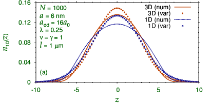
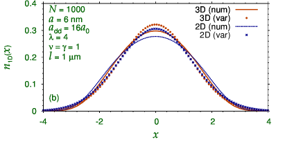
Figure 1: (a) Numerical (num) and variational (var) results for the one-dimensional axial density $n_{1D}(z)=|\phi_{1D}(z)|^{2}$ along $z$ axis for $\nu=\gamma=1,\lambda=0.25$ of a cigar-shaped BEC of $N_{\mathrm{at}}=1000$ atoms obtained using the 1D Eq. (29) and that obtained after integrating the 3D density from Eq. (3) over $x$ and $y$: $n_{1D}(z)=\int|\phi({\bf r})|^{2}dxdy$. (b) Numerical (num) and variational (var) results for the 1D radial density $n_{1D}(x)=\int|\phi({\bf r})|^{2}dydz$ along $x$ axis for $\nu=\gamma=1,\lambda=4$ of a disk-shaped BEC of $N_{\mathrm{at}}=1000$ atoms obtained after integrating the 3D density from Eq. (3) over $y$ and $z$ and after integrating the 2D density from Eq. (46) over $y$ as follows: $n_{1D}(x)=\int dy|\phi_{2D}(x,y)|^{2}$ and $n_{1D}(x)=\int dydz|\phi_{3D}(x,y,z)|^{2}$. In all cases $a=6$ nm and $a_{dd}=16a_{0}$.

The 1D and 2D GP equations (29) and (46) are valid for cigar- and disk-shaped BECs, respectively. In case of cigar shape the 1D GP equation yields results for axial density and in this case it is appropriate to compare this density with the reduced axial density obtained by integrating the 3D density over radial coordinates: $\displaystyle n(z)\equiv|\varphi(z)|^{2}=\int|\phi(x,y,z)|^{2}\,dx\,dy$. In Fig. 1 (a) we compare two axial densities obtained from the 1D and 3D GP equations. We also show the densities calculated from the Gaussian variational approximation in both cases. In the cigar case the trap parameters are $\nu=\gamma=1,\lambda=1/4$. Similarly, for the disk shape it is interesting to compare the density along the radial direction in the plane of the disk as obtained from the 3D equation (3) and the 2D equation (46). In this case it is appropriate to calculate the 1D radial density along, say, $x$ direction by integrating 2D and 3D densities as follows: $n_{1D}(x)=\int dy|\phi_{2D}(x,y)|^{2}$ and $n_{1D}(x)=\int dydz|\phi_{3D}(x,y,z)|^{2}$. In Fig. 1 (b) we compare two radial densities obtained from the 2D and 3D GP equations. We also show the densities calculated from the Gaussian variational approximation in both cases. For this illustration, we consider the trap parameters $\nu=\gamma=1,\lambda=4$. In both Figs. 1 (a) and (b), the densities obtained from the solution of the 3D GP equation are in satisfactory agreement with those obtained from a solution of the reduced 1D and 2D equations. In Fig. 1, the numerical and variational densities are pretty close to each other, so are the results obtained from the 3D equation (3), on the one hand, and the ones obtained from the 1D and 2D equations (29) and (46), on the other.

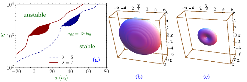
Figure 2: (a) The $N_{\mathrm{at}}-a$ stability phase plot for a ¹⁶⁴Dy BEC with $a_{\mathrm{dd}}=130a_{0}$ in a disk-shaped trap with $\nu=\gamma=1$, $\lambda=5$ and 7 and harmonic oscillator length $l=1$ $\mu$m. The 3D isodensity contour plot of density of a disk-shaped ¹⁶⁴Dy BEC with $a_{\mathrm{dd}}=130a_{0}$ for $\nu=\gamma=1$, $\lambda=5$, $l=1$ $\mu$m, $N_{\mathrm{at}}=3000$ and $a=40a_{0}$ for densities $|\phi(x,y,z)|^{2}$ = (b) 0.001 and (c) 0.027 on the contour.

A dipolar BEC is stable for the number of atoms $N_{\mathrm{at}}$ below a critical value [31]. Independent of trap parameters, such a BEC collapses as $N_{\mathrm{at}}$ crosses the critical value. This can be studied by solving the 3D GP equation using imaginary-time propagation with a nonzero value of NSTP while the nonlinearities are slowly increased. In Fig. 2 (a) we present the $N_{\mathrm{at}}-a$ stability phase plot for a ¹⁶⁴Dy BEC with $a_{\mathrm{dd}}=130a_{0}$ in the disk-shaped trap with $\nu=\gamma=1$, $\lambda=5$ and 7. The oscillator length is taken to be $l=1$ $\mu$m. The shaded area in these plots shows a metastable region where biconcave structure in 3D density appears. The metastable region corresponds to a local minimum in energy in contrast to a global minimum for a stable state. It has been established that this metastability is a manifestation of roton instability encountered by the system in the shaded region [31]. The biconcave structure in 3D density in a disk-shaped dipolar BEC is a direct consequence of dipolar interaction: the dipolar repulsion in the plane of the disk removes the atoms from the center to the peripheral region thus creating a biconcave shape in density. In Figs. 2 (b) and (c) we plot the 3D isodensity contour of the condensate for $\lambda=5$ with parameters in the shaded region corresponding to metastability. In Fig. 2 (b) the density on the contour is 0.001 whereas in Fig. 2 (c), it is 0.027. Only for a larger density on the contour the biconcave shape is visible. The biconcave shape predominates near the central region of the metastable dipolar BEC.

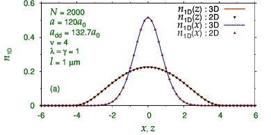
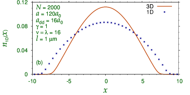
Figure 3: (a) Numerical results for the 1D radial density $n_{1D}(x)=\int|\phi({\bf r})|^{2}dydz$ along $x$ axis and $n_{1D}(z)=\int|\phi({\bf r})|^{2}dxdy$ along $z$ axis for $\lambda=\gamma=1,\nu=4$ of a disk-shaped BEC of $N_{\mathrm{at}}=2000$ ¹⁶⁴Dy atoms obtained after integrating the 3D density from Eq. (3) and the 2D density from Eq. (55) over the eliminated variables. (b) Numerical results for the 1D axial density $n_{1D}(x)=$ along $x$ axis for $\nu=\lambda=16,\gamma=1$ of a cigar-shaped BEC of $N_{\mathrm{at}}=2000$ ⁵²Cr atoms obtained using the 1D Eq. (41) and that obtained after integrating the 3D density from Eq. (3) over $z$ and $y$: $n_{1D}(x)=\int|\phi({\bf r})|^{2}dzdy$. In all cases $a=120a_{0}$ and (a) $a_{dd}=132.7a_{0}$, (b) $a_{dd}=16a_{0}$.

In figure 1 we critically tested the reduced 1D and 2D equations (29) and (46) along the $z$ axis and in the $x-y$ plane, respectively, by comparing the different 1D densities from these equations with those obtained from a solution of the 3D equation (3) as well as with the variational densities. Now we perform a similar test with the reduced 1D and 2D equations (41) and (55) along the $x$ axis and in the $x-z$ plane, respectively. We consider a BEC of 2000 atoms in a disk-shaped trap in the $x-z$ plane with $\lambda=\gamma=1$ and $\nu=4$. Because of the strong trap in the $y$ direction, the resultant BEC is of quasi-2D shape in the $x-z$ plane without circular symmetry in that plane because of the anisotropic dipolar interaction. The integrated linear density along the $x$ and $z$ axes as calculated from the 2D GP equation (55) and the 3D GP equation (3) are illustrated in figure 3 (a). Next we consider the BEC of 2000 atoms in a cigar-shaped trap along the $x$ axis with $\nu=\lambda=16$ and $\gamma=1$. The integrated linear density along the $x$ axis in this case calculated from the 3D equation (3) is compared with the same as calculate using the reduced 1D equation (41) in figure 3 (b). In both cases the densities calculated from the 3D GP equation are in reasonable agreement with those calculated using the reduced equations (55) and (41). Another interesting feature emerges from figures 1 and 3: the reduced 2D GP equations (46) and (55) with appropriate disk-shaped traps yield results for densities in better agreement with the 3D GP equation (3) as compared to the 1D GP equations (29) and (41) with appropriate cigar-shaped traps. This feature, also observed in non-dipolar BECs [17], is expected as the derivation of the reduced 1D equations involving two spatial integrations represent more drastic approximation compared to the same of the reduced 2D equations involving one spatial integration.

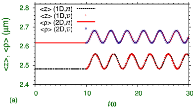
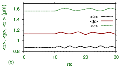
Figure 4: (a) Numerical ($n$) and variational ($v$) results for oscillation of rms sizes $\langle z\rangle$ and $\langle\rho\rangle$ from the real-time simulation using Eq. (29) in 1D and Eq. (46) in 2D, respectively, for $N_{\mathrm{at}}=10000$, $a=6$ nm, $a_{\mathrm{dd}}=16a_{0}$, $l=1$ $\mu$m, while $a$ and $a_{dd}$ were both multiplied by 1.05 after NPAS iterations at $t=10$. The wave function was first calculated by imaginary-time routine with parameters $dx=0.025$, $dt=0.0001,\lambda=1,d_{\rho}=1$, NPAS= $10^{5},N=2048$ in 1D, and $dx=dy=0.2,dt=0.001,\gamma=1,d_{z}=1$ NPAS = 10⁴, $NX=NY=512$ in 2D. The results of the variational approximations in 1D and 2D as obtained from a numerical solution of Eqs. (36) and (50) are also shown. (b) Numerical results for oscillation of rms sizes $\langle x\rangle,\langle y\rangle$ and $\langle z\rangle$ from the real-time simulation in 3D using Eq. (3), for $N_{\mathrm{at}}=1000$, $a=110a_{0}$, $a_{\mathrm{dd}}=16a_{0}$, $l=1$ $\mu$m, $\gamma=1,\nu=1/\sqrt{2},\lambda=1/2$, $NX=NY=NZ=128,dx=dy=dz=0.2$, and $dt=0.002$ while $a$ and $a_{\mathrm{dd}}$ were both multiplied by 1.1 after NPAS iterations. In all cases the real-time calculation was performed with NSTP = 0 reading the 3D density from the numerical solution of the imaginary-time program using the same parameters.

Now we report the dynamics of the dipolar BEC by real-time propagation using the stationary state calculated by imaginary-time propagation. In Fig. 4 (a) we show the oscillation of the rms sizes $\langle z\rangle$ and $\langle\rho\rangle$ from the reduced 1D and 2D GP equations (29) and (46), respectively. In Fig. 4 (a) we consider $N_{\mathrm{at}}=10000,a_{\mathrm{dd}}=16a_{0}$ (appropriate for ⁵²Cr), $a=6$ nm ($\approx 113a_{0}$) and oscillator length $l=1$ $\mu$m. In 1D, we take $dx=0.025,dt=0.0001,\lambda=1,d_{\rho}=1$, number of space points $N=2048$, and in 2D, we take $dx=dy=0.2,dt=0.001,\gamma=\nu=1,d_{z}=1,NX=NY=512.$in real-time simulation the oscillation is started by multiplying the nonliniarities with the factor 1.05. To impliment this, in real-time routine we take GPAR = GDPAR = 1.1 and also take NSTP = 0 to read the initial wave function. In 1D and 2D we also present results of the Gaussian variational approximations after a numerical solution of Eqs. (36) and (50), respectively. The frequency of the resultant oscillations agree well with the numerical 1D and 2D calculations. However, slight adjustment of the initial conditions, or initial values of width and its derivative, were necessary to get an agreement of the amplitude of oscillation obtained from variational approximation and numerical simulation. The initial values of width and its derivative are necessary to solve the variational Eqs. (36) and (50). In Fig. 4 (b) we illustrate the oscillation of the rms sizes $\langle x\rangle$, $\langle y\rangle$, and $\langle z\rangle$ in 3D using Eq. (3), where we perform real-time simulation using the bound state obtained by imaginary-time simulation as the initial state. The parameters used are $N_{\mathrm{at}}=1000,a=110a_{0},a_{\mathrm{dd}}=16a_{0},\gamma=1,\nu=1/\sqrt{2},\lambda=1/2,l=1$ $\mu$m, $NX=NY=NZ=128,dx=dy=dz=0.2,dt=0.002$ in both real- and imaginary-time simulations. In addition, in real-time simulation the oscillation is started by multiplying the nonliniarities with the factor 1.1. To impliment this, in real-time routine we take GPAR = GDPAR = 1.1 and also take NSTP = 0 to read the initial wave function.

5 Summary

We have presented useful numerical programs in Fortran and C for solving the dipolar GP equation including the contact interaction in 1D, 2D, 3D. Two sets of programs are provided. The imaginary-time programs are appropriate for solving the stationary problems, while the real-time codes can be used for studying non-stationary dynamics. The programs are developed in Cartesian coordinates. We have compared the results of numerical calculations for statics and dynamics of dipolar BECs with those of Gaussian variational approximation, Thomas-Fermi approximation, and numerical calculations of other authors, where possible.

References

- [1] F. Dalfovo, S. Giorgini, L. P. Pitaevskii, S. Stringari, Theory of Bose-Einstein condensation in trapped gases, Rev. Mod. Phys. 71 (1999) 463-512; A.J. Leggett, Bose-Einstein condensation in the alkali gases: Some fundamental concepts, Rev. Mod. Phys. 73 (2001) 307–356; L. Pitaevskii, S. Stringari, Bose-Einstein Condensation, Clarendon Press, Oxford and New York, 2003; C.J. Pethick, H. Smith, Bose-Einstein Condensation in Dilute Gases, Cambridge University Press, Cambridge, 2002.
- [2] S. K. Adhikari, P. Muruganandam, Bose-Einstein condensation dynamics from the numerical solution of the Gross-Pitaevskii equation, J. Phys. B 35 (2002) 2831; P. Muruganandam, S. K. Adhikari, Bose-Einstein condensation dynamics in three dimensions by the pseudospectral and finite-difference methods, J. Phys. B 36 (2003) 2501; S.K. Adhikari, Numerical study of the spherically symmetric Gross-Pitaevskii equation in two space dimensions, Phys. Rev. E 62 (2000) 2937–2944; S.K. Adhikari, Numerical solution of the two-dimensional Gross-Pitaevskii equation for trapped interacting atoms, Phys. Lett. A 265 (2000) 91–96.
- [3] P. Muruganandam, S. K. Adhikari, Fortran programs for the time-dependent Gross-Pitaevskii equation in a fully anisotropic trap, Comput. Phys. Commun. 180 (2009) 1888-1912.
- [4] D. Vudragović, I. Vidanović, A. Balaž, P. Muruganandam, S. K. Adhikari, C programs for solving the time-dependent Gross-Pitaevskii equation in a fully anisotropic trap, Comput. Phys. Commun. 183 (2012) 2021-2025.
- [5] W. Wen, C. Zhao, X. Ma, Dark-soliton dynamics and snake instability in superfluid Fermi gases trapped by an anisotropic harmonic potential Phys. Rev. A 88 (2013) 063621; K.-T. Xi, J. Li, D.-N. Shi, Localization of a two-component Bose-Einstein condensate in a two-dimensional bichromatic optical lattice, Physica B-Cond. Mat. 436 (2014) 149-156; Y.-S. Wang, Z.-Y. Li, Z.-W. Zhou, X.-F. Diao, Symmetry breaking and a dynamical property of a dipolar Bose-Einstein condensate in a double-well potential, Phys. Lett. A 378 (2014) 48-52; E. J. M. Madarassy, V. T. Toth, Numerical simulation code for self-gravitating Bose-Einstein condensates, Comput. Phys. Commun. 184 (2013) 1339-1343; R. M. Caplan, NLSEmagic: Nonlinear Schrödinger equation multi-dimensional Matlab-based GPU-accelerated integrators using compact high-order schemes, Comput. Phys. Commun. 184 (2013) 1250-1271; I. Vidanovic, A. Balaž, H. Al-Jibbouri, A. Pelster, Nonlinear Bose-Einstein-condensate dynamics induced by a harmonic modulation of the s-wave scattering length, Phys. Rev. A 84 (2011) 013618; Y. Cai, H. Wang, Analysis and computation for ground state solutions of Bose-Fermi mixtures at zero temperature, Siam J. App. Math. 73 (2013) 757-779; A. Balaž, R. Paun, A. I. Nicolin, S. Balasubramanian, R. Ramaswamy, Faraday waves in collisionally inhomogeneous Bose-Einstein condensates, Phys. Rev. A 89 (2014) 023609; H. Al-Jibbouri, A. Pelster, Breakdown of the Kohn theorem near a Feshbach resonance in a magnetic trap, Phys. Rev. A 88 (2013) 033621; E. Yomba, G.-A. Zakeri, Solitons in a generalized space- and time-variable coefficients nonlinear Schrödinger equation with higher-order terms, Phys. Lett. A 377 (2013) 2995-3004; X. Antoine, W. Bao, C. Besse, Computational methods for the dynamics of the nonlinear Schrödinger/Gross-Pitaevskii equations, Comput. Phys. Commun. 184 (2013) 2621-2633; N. Murray et al., Probing the circulation of ring-shaped Bose-Einstein condensates, Phys. Rev. A 88 (2013) 053615; A. Khan, P. K. Panigrahi, Bell solitons in ultra-cold atomic Fermi gas, J. Phys. B 46 (2013) 115302; E. Yomba, G.-A. Zakeri, Exact solutions in nonlinearly coupled cubic-quintic complex Ginzburg-Landau equations, Phys. Lett. A 377 (2013) 148-157; W. Bao, Q. Tang, Z. Xu, Numerical methods and comparison for computing dark and bright solitons in the nonlinear Schrödinger equation, J. Comput. Phys. 235 (2013) 423-445; W. Wen, H.-J. Li, Interference between two superfluid Fermi gases, J. Phys. B 46 (2013) 035302; H. Zheng, Y. Hao, Q. Gu, Dynamics of double-well Bose-Einstein condensates subject to external Gaussian white noise, J. Phys. B 46 (2013) 065301; Y. Wang, F.-D. Zong, F.-B. Li, Three-dimensional Bose-Einstein condensate vortex solitons under optical lattice and harmonic confinements, Chinese Phys. B. 22 (2013) 030315; P.-G. Yan, S.-T. Ji, X.-S. Liu, Symmetry breaking and tunneling dynamics of F=1 spinor Bose-Einstein condensates in a triple-well potential, Phys. Lett. A 377 (2013) 878-884; R. R. Sakhel, A. R. Sakhel, H. B. Ghassib, Nonequilibrium Dynamics of a Bose-Einstein Condensate Excited by a Red Laser Inside a Power-Law Trap with Hard Walls, J. Low Temp. Phys 173 (2013) 177-206; A. Trichet, E. Durupt, F. Médard, S. Datta, A. Minguzzi, and M. Richard, Long-range correlations in a 97 excitonic one-dimensional polariton condensate, Phys. Rev. B 88 (2013) 121407; X. Yue et al., Observation of diffraction phases in matter-wave scattering, Phys. Rev. A 88 (2013) 013603; S. Prabhakar et al., Annihilation of vortex dipoles in an oblate Bose-Einstein condensate, J. Phys. B 46 (2013) 125302; Z. Marojevic, E. Goeklue, C. Laemmerzahl, Energy eigenfunctions of the 1D Gross-Pitaevskii equation, Comput. Phys. Commun. 184 (2013) 1920-1930; T. Mithun, K. Porsezian, B. Dey, Vortex dynamics in cubic-quintic Bose-Einstein condensates, Phys. Rev. E 88 (2013) 012904; M. Edwards, M. Krygier, H. Seddiqi, B. Benton, and C. W. Clark, Approximate mean-field equations of motion for quasi-two-dimensional Bose-Einstein-condensate systems, Phys. Rev. E 86 (2012) 056710; J. Li, F.-D. Zong, C.-S. Song, Y. Wang, and F.-B. Li, Dynamics of analytical three-dimensional solutions in Bose-Einstein condensates with time-dependent gain and potential, Phys. Rev. E 85 (2012) 036607; P. Verma, A. B. Bhattacherjee, M. Mohan, Oscillations in a parametrically excited Bose-Einstein condensate in combined harmonic and optical lattice trap, Central Eur. J. Phys. 10 (2012) 335-341; E. R. F. Ramos, F. E. A. dos Santos, M. A. Caracanhas, and V. S. Bagnato, Coupling collective modes in a trapped superfluid, Phys. Rev. A 85 (2012) 033608; W. B. Cardoso, A. T. Avelar, D. Bazeia, Modulation of localized solutions in a system of two coupled nonlinear Schrödinger equations, Phys. Rev. E 86 (2012) 027601; P.-G. Yan, Y.-S. Wang, S.-T Ji, X.-S. Liu, Symmetry breaking of a Bose-Fermi mixture in a triple-well potential, Phys. Lett. A 376 (2012) 3141-3145; H. L. Zheng, Y. J. Hao, Q. Gu, Dissipation effect in the double-well Bose-Einstein condensate, Eur. Phys. J. D 66 (2012) 320; P. Verma, A. B. Bhattacherjee, M. Mohan, Oscillations in a parametrically excited Bose-Einstein condensate in combined harmonic and optical lattice trap, Central Eur. J. Phys. 10 (2012) 335-341; W. B. Cardoso, A. T. Avelar, D. Bazeia, One-dimensional reduction of the three-dimenstional Gross-Pitaevskii equation with two- and three-body interactions, Phys. Rev. E 83 (2011) 036604; R. R. Sakhel, A. R. Sakhel, H. B. Ghassib, Self-interfering matter-wave patterns generated by a moving laser obstacle in a two-dimensional Bose-Einstein condensate inside a power trap cut-off by box potential boundaries, Phys. Rev. A 84 (2011) 033634; A. Balaž, A. I. Nicolin, Faraday waves in binary nonmiscible Bose-Einstein condensates, Phys. Rev. A 85 (2012) 023613; S. Yang, M. Al-Amri, J. Evers, M. S. Zubairy, Controllable optical switch using a Bose-Einstein condensate in an optical cavity, Phys. Rev. A 83 (2011) 053821; Z. Sun, W. Yang, An exact short-time solver for the time-dependent Schrödinger equation, J. Chem. Phys. 134 (2011) 041101; G. K. Chaudhary, R. Ramakumar, Collapse dynamics of a (176)Yb-(174)Yb Bose-Einstein condensate, Phys. Rev. A 81 (2010) 063603; S. Gautam, D. Angom, Rayleigh-Taylor instability in binary condensates, Phys. Rev. A 81 (2010) 053616; S. Gautam, D. Angom, Ground state geometry of binary condensates in axisymmetric traps, J. Phys. B 43 (2010) 095302; G. Mazzarella, L. Salasnich, Collapse of triaxial bright solitons in atomic Bose-Einstein condensates, Phys. Lett. A 373 (2009) 4434-4437;
- [6] T. Koch, T. Lahaye, Fröhlich, A. Griesmaier, T. Pfau, Stabilization of a purely dipolar quantum gas against collapse, Nature Phys. 4 (2008) 218-222.
- [7] M. Lu, N. Q. Burdick, Seo Ho Youn, B. L. Lev, Strongly Dipolar Bose-Einstein Condensate of Dysprosium, Phys. Rev. Lett. 107 (2011) 190401.
- [8] K. Aikawa et al., Bose-Einstein Condensation of Erbium, Phys. Rev. Lett. 108 (2012) 210401.
- [9] W. Bao, Y. Cai, H. Wang, Efficient numerical methods for computing ground states and dynamics of dipolar Bose-Einstein condensates, J. Comput. Phys. 229 (2010) 7874-7892.
- [10] S. Yi, L. You, Trapped condensates of atoms with dipole interactions, Phys. Rev. A 63 (2001) 053607; Quantum Phases of Dipolar Spinor Condensates, S. Yi, L. You, and H. Pu, Phys. Rev. Lett. 93 (2004) 040403.
- [11] K. Góral, L. Santos, Ground state and elementary excitations of single and binary Bose-Einstein condensates of trapped dipolar gases, Phys. Rev. A 66 (2002) 023613.
- [12] S. Ronen, D. C. E. Bortolotti, J. L. Bohn, Bogoliubov modes of a dipolar condensate in a cylindrical trap, Phys. Rev. A 74 (2006) 013623.
- [13] P. B. Blakie, C. Ticknor, A. S. Bradley, A. M. Martin, M. J. Davis, Y. Kawaguchi, Numerical method for evolving the dipolar projected Gross-Pitaevskii equation, Phys. Rev. E 80 (2009) 016703.
- [14] T. Lahaye, J. Metz, B. Fröhlich, T. Koch, M. Meister, A. Griesmaier, T. Pfau, H. Saito, Y. Kawaguchi, and M. Ueda, -Wave Collapse and Explosion of a Dipolar Bose-Einstein Condensate, Phys. Rev. Lett. 101 (2008) 080401.
- [15] N. G. Parker, C. Ticknor, A. M. Martin, D. H. J. O’Dell, Structure formation during the collapse of a dipolar atomic Bose-Einstein condensate, Phys. Rev. A 79 (2009) 013617; C. Ticknor, N. G. Parker, A. Melatos, S. L. Cornish, D. H. J. O’Dell, A. M. Martin, Collapse times of dipolar Bose-Einstein condensate, Phys. Rev. A 78 (2008) 061607.
- [16] M. Asad-uz-Zaman, D. Blume, Aligned dipolar bose-einstein condensate in a double-well potential: From cigar shaped to pancake shaped, Phys. Rev. A 80 (2009) 053622.
- [17] L. Salasnich, A. Parola, and L. Reatto, Effective wave equations for the dynamics of cigar-shaped and disk-shaped Bose condensates, Phys. Rev. A 65 (2002) 043614.
- [18] L. Santos, V. Shylapnikov, G, P. Zoller, M. Lewenstein, Bose-Einstein condensation in trapped dipolar gases, Phys. Rev. Lett. 85 (2000) 1791-1794.
- [19] T Lahaye, C Menotti, L Santos, M Lewenstein, T Pfau, The physics of dipolar bosonic quantum gases, Rep. Prog. Phys. 72 (2009) 126401.
- [20] V. M. Pérez-García, H. Michinel, J. I. Cirac, M. Lewenstein, and P. Zoller Phys. Rev. A 56 (1997) 1424-1432.
- [21] S. Giovanazzi, A. Görlitz, T. Pfau, Ballistic expansion of a dipolar condensate, J. Opt. B 5 (2003) S208-S211.
- [22] P. Muruganandam, S. K. Adhikari, Numerical and variational solutions of the dipolar Gross-Pitaevskii equation in reduced dimensions, Laser Phys. 22 (2012) 813-820.
- [23] D. O’Dell, S. Giovanazzi, C. Eberlein, Exact Hydrodynamics of a dipolar Bose-Einstein condensate, Phys. Rev. Lett. 92 (2004) 250401.
- [24] C. Eberlein, S. Giovanazzi, D. H. J. O’Dell, Exact solution of the Thomas-Fermi equation for a trapped Bose-Einstein condensate with dipole-dipole interactions, Phys. Rev. A 71 (2005) 033618.
- [25] N. G. Parker, D. H. J. O’Dell, Thomas-Fermi versus one- and two-dimensional regimes of a trapped dipolar Bose-Einstein condensate, Phys. Rev. A. 78 (2008) 41601(R).
- [26] S. Sinha, L. Santos, Cold dipolar gases in quasi-one-dimensional geometries, Phys. Rev. Lett. 99 (2007) 140406; F. Deuretzbacher, J. C. Cremon, S. M. Reimann, Ground-state properties of few dipolar bosons in a quasi-one-dimensional harmonic trap, Phys. Rev. A 81 (2010) 063616.
- [27] S. Giovanazzi, D. H. J. O’Dell, Eur. Phys. J. D 31 (2004) 439-445.
- [28] U. R. Fischer, Stability of quasi-two-dimensional Bose-Einstein condensates with dominant dipole-dipole interactions, Phys. Rev. A 73 (2006) 031602; P. Pedri, L. Santos, Two-Dimensional Bright Solitons in Dipolar Bose-Einstein Condensates, Phys. Rev. Lett. 95 (2005) 200404.
- [29] M. Asad-uz-Zaman, D. Blume, private communication (2010).
- [30] A. Aftalion, Q. Du, Vortices in a rotating Bose–Einstein condensate: Critical angular velocities and energy diagrams in the Thomas-Fermi regime, Phys. Rev. A 64 (2001) 063603.
- [31] S. Ronen, D. C. E. Bortolotti, J. L. Bohn, Radial and Angular Rotons in Trapped Dipolar Gases, Phys. Rev. Lett. 98 (2007) 030406; R. M. Wilson, S. Ronen, J. L. Bohn, H. Pu, Manifestations of the Roton Mode in Dipolar Bose-Einstein Condensates, Phys. Rev. Lett. 100, (2008) 245302; L. Santos, G. V. Shlyapnikov, M. Lewenstein, Roton-Maxon Spectrum and Stability of Trapped Dipolar Bose-Einstein Condensates, Phys. Rev. Lett. 90 (2003) 250403; M. Asad-uz-Zaman, D. Blume, Modification of roton instability due to the presence of a second dipolar Bose-Einstein condensate, Phys. Rev. A 83 (2011) 033616.