Protocol-independent granular temperature supported by numerical simulations

Abstract

A possible approach to the statistical description of granular assemblies starts from Edwards’ assumption that all blocked states occupying the same volume are equally probable (S.F. Edwards, R. Oakeshott, Physica A 157, 1080 (1989)). We performed computer simulations using two-dimensional polygonal particles excited periodically according to two different protocols: excitation by pulses of “negative gravity” and excitation by “rotating gravity”. The first protocol exhibits a non-monotonous dependency of the mean volume fraction on the pulse strength. The overlapping histogram method is used in order to test whether or not the volume distribution is described by a Boltzmann-like distribution, and to calculate the inverse compactivity as well as the logarithm of the partition sum. We find that the mean volume is a unique function of the measured granular temperature, independently of the protocol and of the branch in $\phi(g)$, and that all determined quantities are in agreement with Edwards’ theory.

I Introduction

Granular materials are typically composed of thousands to millions of individual particles (or more). Think for example of the cereals for breakfast or of the sand on the shore. These large numbers suggest that statistical methods may be applicable and constitute a powerful tool in developing a better theoretical understanding of these kinds of materials. However, contrary to the situation in gases or fluids, where the permitted phase space is explored continuously due to chaotic molecular motion, thermal fluctuations are negligible for granular materials. Furthermore, the particle dynamics are dissipative. Therefore, it is not possible to carry standard statistical mechanics over to granular assemblies. In particular, the classical Boltzmann distribution, where the probability of a state is inversely proportional to the exponential of its energy (measured in units of $k_{B}T$), will not apply to these systems.

Edwards and Oakeshott Edwards and Oakeshott (1989a, b) proposed that concepts from classical statistical mechanics are applicable, if one assumes that the volume of a static, stable granulate plays the same role in granular statistics as the energy of a microstate in classical statistics. This means that, analogous to the classical microcanonical ensemble, where all states with the same energy are equally probable, all mechanically stable configurations of the granular assembly that occupy the same volume occur with the same probability. The entropy of this granular microcanonical ensemble is proportional to the logarithm of the number of blocked states with a certain volume. By analogy with classical statistics, one can define a temperature-like variable, called compactivity, as the inverse of the derivative of the Edwards entropy with respect to the volume. Later, it turned out that for a full description of a granular system, beyond the volume ensemble also an ensemble for the different stress states must be introduced Bi et al. (2015); Henkes et al. (2007); Blumenfeld and Edwards (2006) and that the volume and the stress ensembles are probably interdependent Blumenfeld et al. (2012). However, it seems that expectation values of quantities that depend on the geometrical state only and not on the stress state are well described by the volume ensemble Blumenfeld and Edwards (2014), possibly because the force-moment tensor can be treated as approximately constant in the systems considered here. Therefore we focus on the volume ensemble in most of the present paper.

Some doubts about the temperature-like interpretation of the compactivity have been raised on the basis of equilibration experiments performed by Puckett and Daniels Puckett and Daniels (2013). They found that in a two-component system, the compactivity did not equilibrate, whereas the angoricity did. There are different ways to explain this observation, some of which do not necessitate to give up the interpretation of the compactivity as a temperature-like variable .

A key assumption of standard statistical mechanics is the equivalence of time and ensemble averages, but mechanically stable granular configurations are static states without any intrinsic time evolution. On the other hand, by applying the same external excitation to the granular material again and again (i.e. tapping Nowak et al. (1998) or shearing Tsai et al. (2003)), this external excitation may take over the role of thermal agitation and the concept of a time average becomes meaningful for granular statistics as well. Some tests of the ergodicity of granular systems are available in the literature. With systems of frictional discs excited with flow pulses, equivalence between time and ensemble averages was found Ciamarra et al. (2006). In the case of a vertical tapping protocol, dependency on the protocol parameters was noted. Especially for small tapping amplitudes, nonergodicity was observed in numerical simulations Paillusson and Frenkel (2012). This may be related to the occurrence of irreversible branches in tapped granular systems Nowak et al. (1998); Pugnaloni et al. (2008).

Several methods were proposed to determine the compactivity from experimental or simulation data Nowak et al. (1998); Schröter et al. (2005); Zhao et al. (2012); Zhao and Schröter (2014) and applied to different kinds of granulates. In this work, we employ two-dimensional discrete-element (DEM) simulations using polygonal particles to apply two different excitation protocols to otherwise identical granulates. This allows us to determine whether the calculated compactivity is independent of the specific excitation protocol (which would support the Edwards theory) or not (which would oppose it). Recently, some authors have addressed the issue whether or not it is necessary to introduce protocol specific extensions of Edwards-like approaches Paillusson (2015); Asenjo et al. (2014). We briefly discuss a possible approach in section II.2. At least for the two protocols considered in this paper, we find protocol independence. Furthermore, we test whether ideal-gas-like prediction analogies of the Edwards theory are consistent with the simulation data, and find good qualitative agreement, which even becomes quantitative if certain parameters are chosen by fitting.

The paper is organized as follows. In section II, we give an overview of some aspects of Edwards’ theory, relevant to this work. In section III, we introduce the simulation technique. Section IV gives details of the applied excitation protocols and in section V, the simulation results will be presented, evaluated and discussed. In Sec. VI, some limitations of the volume ensemble are illustrated. Finally, section VII gives a summary of our findings.

II Theoretical framework

II.1 The microcanonical and the canonical volume ensemble

The main assumption of the Edwards theory is the following Edwards and Oakeshott (1989a, b): If a granular ensemble is generated by a reproducible preparation protocol, all resulting mechanically stable configurations of the granular system which occupy the same volume will occur with the same probability on repetition of the protocol. This means that in Edwards’ granular statistics the volume plays the same role as the energy in ordinary statistics. Consequently, the entropy $S$ of the microcanonical ensemble having a certain volume $V$ is given as the logarithm of the number $\Omega$ of stable states (in the permitted phase space) occupying this volume.

Let a microstate of the granular ensemble, comprised of $N$ particles, be described by a set of variables $\bm{q}$. The entropy of this state is given by (see e. g. Edwards and Oakeshott (1989a, b); Blumenfeld and Edwards (2014)):

$$S(V,N) =\ln\Omega(V,N)\>,$$ (1)

$$\Omega(V,N) =\int_{\{\bm{q}\}}\mathrm{d}\bm{q}~{}\delta(V-W(\bm{q}))\>.$$ (2)

The integral runs over all stable configurations $\{\bm{q}\}$ and the function $W(\bm{q})$ gives the volume of the state $\bm{q}$. Note that in this context, $W(\bm{q})$ is the granular analogue of the Hamiltonian and $V$ is the analogue of the internal energy.

By analogy with standard statistical mechanics, an intensive, temperature-like variable $\chi$ can be defined, usually called compactivity:

$$\chi=\beta^{-1}=\frac{\partial{V}}{\partial{S}}\>.$$ (3)

In this paper, we will, for simplicity, mostly use the “thermodynamic beta”, defined as the inverse compactivity $\beta=1/\chi$, instead of the compactivity itself.

Note that in general, a constant $\lambda$ analogous to the Boltzmann constant may be introduced in (1) and (3). Here, we use $\lambda=1$ which means that we measure compactivity in units of volume.

As in ordinary statistics/thermodynamics (see e.g. Landau and Lifschitz (1987)) one may switch from the microcanonical ensemble to the canonical ensemble by a Legendre transformation. In the corresponding canonical ensemble, the probability of a microstate $\bm{q}$ occupying the volume $W(\bm{q})$ is given by a Boltzmann-like distribution:

$$P(\bm{q})=\frac{1}{Z}e^{-\beta W(\bm{q})}$$ (4)

with the canonical partition function Lechenault et al. (2006); Blumenfeld et al. (2012); Zhao and Schröter (2014)

$$Z=\int_{\{q\}}\mathrm{d}\bm{q}~{}e^{-\beta W(\bm{q})}\>.$$ (5)

Once again, the integral runs over all possible mechanically stable states. Note that this is equivalent to a notation often used in the literature, where the integral runs over all states and contains an additional factor $\theta(\bm{q})$, which takes the value zero for forbidden states and one for allowed ones, thus selecting the permitted states.

Note that a tapping protocol does not necessarily lead to canonical sampling of the system. A trivial example would be tapping with so small an amplitude that the system is trapped in the initial blocked state. A non-trivial example is the irreversible branch for vertical tapping observed by Nowak et. al. Nowak et al. (1998). Also, the comparison between the analytically solvable Bowles-Ashwin model system Bowles and Ashwin (2011) and simulations where such a system is vertically tapped Irastorza1 et al. (2013) exhibits deviations from the canonical ensemble prediction. Note that the Bowles-Ashwin model assumes a highly confined geometry with much lower complexity than realistic granular systems. Vertical tapping applied to this special system with strong confinement may be unsuited for phase space exploration according to a flat probability measure. Or else the flat Edwards measure does not hold in general. Even if that were the case, a meaningful definition of compactivity might still be possible as will be described now.

II.2 Generalised (protocol dependent) ensembles

In case it turned out that Edwards’ assumption of a flat probability measure is not satisfied for the microcanical ensemble, it is possible to modify the ensemble with (in general, state and protocol dependent) weighting factors $w(\bm{q})$ Asenjo et al. (2014); Bi et al. (2015); Paillusson (2015). The microcanical state density would be modified as follows

$$\Omega_{G}(V,N)=\int_{\{\bm{q}\}}\mathrm{d}\bm{q}~{}w(\bm{q})\delta(V-W(\bm{q}))\>.$$ (6)

Providing we have

$$\Omega_{G}(V_{1}+V_{2},N)=\Omega_{G}(V_{1},N_{1})\,\Omega_{G}(V_{2},N_{2})\>,$$ (7)

which is a much weaker assumption than a flat probability measure Bi et al. (2015), it is still possible to define a compactivity. The canonical formulation for the volume ensemble then reads

$$P(\bm{q}) =w(\bm{q})\frac{1}{Z}e^{-\beta W(\bm{q})}\>,$$ (8)

$$Z_{G} =\int_{\{q\}}\mathrm{d}\bm{q}~{}w(\bm{q})e^{-\beta W(\bm{q})}\>.$$ (9)

A similar approach is feasible for the force-moment and the combined ensembles. Generalised canonical ensembles of this kind are used in statistical genetics Nourmohammad et al. (2013); Barton and Coe (2009).

The qualitative impact of these modifications on the resulting thermodynamics is small. Especially equations (17) and (20) remain unaffected, as long as the weighting factors are the same for all data samples. If only one protocol is used, it is impossible to detect protocol dependencies in the weighting factors. But a comparison of different protocols, applied to the same system, may help to decide whether these factors, if their introduction should turn out necessary, are protocol independent or not.

II.3 Mean volume and volume fluctuations

The calculation of the mean volume and its fluctuations is straightforward. The first derivative of the logarithm of (5) (or (9)) with respect to $\beta$ essentially is the mean volume

$$\langle V\rangle=-\frac{\partial{}}{\partial{\beta}}\ln Z=\frac{1}{Z}\int_{\{q\}}\mathrm{d}\bm{q}~{}W(\bm{q})e^{-\beta W(\bm{q})}\>,$$ (10)

whereas its second derivative is the variance of the volume distribution, i.e., a measure for the strength of fluctuations.

$$\sigma_{V}^{2} =\langle V^{2}\rangle-\langle V\rangle^{2}=\frac{\partial^{2}{}}{\partial{\beta^{2}}}\ln Z\>,$$ (11)

$$\sigma_{V}^{2} =-\frac{\partial{}}{\partial{\beta}}\langle V\rangle\>.$$ (12)

Instead of the volume itself, we use the the volume fraction $\phi$, defined as the sum of the grain volumes $V_{g}$ divided by the volume $W$ occupied by the granulate:

$$\phi(\bm{q})=\frac{V_{g}}{W(\bm{q})}\>.$$ (13)

The volume $W(\bm{q})$ of a certain state can be written as a sum of the mean volume $V=\langle W\rangle$ and the deviation from the mean: $W=V+\Delta V$. Under the assumption that the volume fluctuations are small compared to the mean volume, we can write:

$$\phi=\frac{V_{g}}{V+\Delta V}\simeq\frac{V_{g}}{V}-\frac{V_{g}}{V^{2}}\Delta V\>.$$ (14)

The mean volume fraction is therefore:

$$\bar{\phi}=\langle\phi\rangle=\frac{V_{g}}{V}\>,$$ (15)

and from eqs. (14,15), together with $\langle\Delta V^{2}\rangle=\sigma_{V}^{2}$, we obtain

$$\sigma^{2}_{\phi}=\langle(\phi-\bar{\phi})^{2}\rangle=\frac{\langle\phi\rangle^{4}}{V_{g}^{2}}\sigma_{V}^{2}\>.$$ (16)

Substituting $\sigma_{V}^{2}$ from eq. (12) and reexpressing the differential of $\langle V\rangle$ according to $d\langle V\rangle=-V_{g}/\langle V\rangle^{2}d\bar{\phi}$, we find a relation between the mean volume fraction and its fluctuations:

$$\sigma_{\phi}^{2}=\frac{\bar{\phi}^{2}}{V_{g}}\frac{\partial{\bar{\phi}}}{\partial{\beta}}\>.$$ (17)

Measuring the volume fraction fluctuations as a function of the mean volume fraction and integrating equation (17) or (12), respectively, is a way to calculate the compactivity up to an unknown constant. It is used frequently, e.g., in Nowak et al. (1998); Schröter et al. (2005); Zhao and Schröter (2014). Note that determining the granular temperature via eq. (12) or eq. (17) is just a rule of calculation, provided by Edwards’ theory but no proof of the theory. On the other hand, if after determining $\beta$ in some different way the relationship (17) linking it with the volume fraction were not satisfied, a contradiction to Edwards’ theory would have been demonstrated.

II.4 Overlapping histogram method

Another way to determine the inverse compactivity is the overlapping histogram method proposed in 2003 by Dean and Lefèvre Dean and Lefevre (2003). This method may also be used as a test whether or not a distribution of blocked states is Boltzmann-like distributed. In the original paper, the method was applied to the energy of the Sherrington-Kirkpatrick model for spin glasses, driven by a tapping-like mechanism, which has some similarities to granular dynamics. The method was then frequently used to determine the granular temperature Zhao and Schröter (2014); McNamara et al. (2009); Ciamarra et al. (2012); Puckett and Daniels (2013). Under the assumption that Edwards’ theory holds, the probability to measure a certain volume V in a granulate with an inverse compactivity $\beta_{0}$ and a fixed number of grains $N$ is

$$P(V,\beta_{0},N) =\int_{\{\bm{q}\}}\mathrm{d}\bm{q}~{}\delta(V-W(\bm{q}))\frac{1}{Z(\beta_{0},N)}e^{-\beta_{0}W(\bm{q})}$$

$$=\frac{\mathfrak{D}(V,N)}{Z(\beta_{0},N)}e^{-\beta_{0}V}\>,$$ (18)

where $\mathfrak{D}(V,N)$ is the number of blocked states with volume $V$, i.e $\mathfrak{D}(V,N)=\Omega(V,N)$. This equation holds even for the generalised non-flat probability measure approach, when eq. (6) is used for $\Omega(V,N)$.

We define the quantity $Q$ as the logarithm of the ratio of probability densities for the volume $V$ to arise, on the one hand at an inverse compactivity $\beta_{1}$ and on the other hand, in a reference system held at a different inverse compactivity $\beta_{0}$:

$$Q :=\ln\frac{P(V,\beta_{1},N)}{P(V,\beta_{0},N)}\>,$$ (19)

$$Q =\underbrace{(\beta_{0}-\beta_{1})}_{:=A_{10}}V+\underbrace{\ln\frac{Z(\beta_{0},N)}{Z(\beta_{1},N)}}_{:=B_{10}}$$ (20)

Therefore, if we measure the probability density $P(V,\beta,N)$ for different compactivities and calculate $Q(V)$, the resulting function must be linear if Edwards’ theory holds. Evaluating the slope $A_{10}$ allows us to determine the inverse compactivity up to an additive constant. Furthermore, the intercept $B_{10}$ is nothing else than the logarithm of the partition function up to an additive constant at the corresponding inverse compactivity. This permits testing the validity of Edwards’ assumption in the sense, that if $Q(V)$ were not a straight line, neither Eq. (4) nor Eq. (8) would describe the probability density of the system correctly.

However, one has to be somewhat careful with the interpretation of the results, as has been pointed out in McNamara et al. (2009). Under certain circumstances, very similar results as the ones expected from Edwards’ theory can occur, if the distributions of the samples are just Gaussian. In appendix A, we discuss this situation.

II.5 Ideal quadron solution

There are very few real ab initio predictions from Edwards’ theory in the literature Blumenfeld and Edwards (2003); Blumenfeld et al. (2012); Lechenault et al. (2006); Aste and Matteo (2008), due to some general difficulties. In order to calculate analytical expressions for the partition function, knowledge of an explicit expression for the granular Hamiltonian $W(\bm{q})$ is necessary. Of course, if all positions, orientations and shapes of the grains are known, the occupied volume is a function of these quantities, but in practice it is not easy to write down an explicit equation and even if this can be done, the integration over the permitted blocked states is very difficult because the permitted states are unknown in general.

Therefore, attempts to calculate the partition function were based on standard volume tessellations, such as the Voronoi and Delaunay tessellations Voronoi (1908); Delaunay (1934); Aste and Matteo (2008); Aste et al. (2007). A possible alternative is an arch-based approach Slobinsky and Pugnaloni (2015) which a priori takes only stable configurations into account. Blumenfeld and Edwards proposed a physically motivated tessellation based on the quadron construction Ball and Blumenfeld (2002); Blumenfeld and Edwards (2003, 2006, 2014). In principle, quadrons are used as quasi-particles describing the structure of the granulate at any arbitrary position within the system in a distinct way. It was mentioned in the literature that the ideal quadron tesselation fails in the presence of non-convex voids in the granulate Ciamarra (2007). However, in a system of monodisperse spheres such non-convex voids vanish by neglecting rattlers Blumenfeld and Edwards (2007). Even if some non-convex voids remain, they could be tesselated by convex polygons which repairs the quadron tessellation, at the price that the number of quadrons increases. As long as non-convex voids are the exception rather than the rule, they will not produce significant changes to the calculations.

Under the (very rough) assumption that quadrons occupy volumes between $V_{0}-\Delta$ and $V_{0}+\Delta$ at constant density of states and that there are no interactions between the quadrons, the partition function can be calculated explicitly for two dimensional systems (see Blumenfeld and Edwards (2003)):

$$Z=\left(\frac{\sinh(\beta\Delta)}{\beta\Delta}e^{-\beta V_{0}}\right)^{N\bar{z}},$$ (21)

where $N$ is the number of particles and $\bar{z}$ is the mean coordination number in the granular system. This approximation is called the ideal quadron approximation by analogy with the description of ideal gases in ordinary statistics. Note that the partition function (21) is a special version of a more general ideal-gas-like approach. If one assumes that the volume is tesselated by a number $\tilde{N}$ of statistically independent, non-interacting elementary cells and their volume is restricted to an interval between a minimal volume $V_{0}-\Delta$ and a maximal volume $V_{0}+\Delta$, without any additional assumption on the nature of these elementary cells one ends up with Eq. (21), on replacing $N\bar{z}\rightarrow\tilde{N}$. Contrary to the very general ideal-gas-like approach, there are some possibilities to go beyond the interaction-free situation in the quadron approach, which will be considered in future work.

Using (10), the ideal quadron prediction for the mean volume is obtained:

$$\langle V\rangle=N\bar{z}\left(V_{0}+\frac{1}{\beta}-\Delta\coth(\beta\Delta)\right).$$ (22)

For the current work, it is helpful to rewrite (22) in terms of the volume fraction. Dividing (22) by the total grain volume $V_{g}$ results in

$$\bar{\phi}^{-1}=\frac{N\bar{z}V_{0}}{V_{g}}+\frac{N\bar{z}}{V_{g}\beta}-\frac{N\bar{z}\Delta}{V_{g}}\coth(\beta\Delta)\>.$$ (23)

In order to specify the free parameters $V_{0}$ and $\Delta$, we assume that the limits of $\bar{\phi}^{-1}$ can be identified with the volume fractions of random loose packing (rlp) and random close packing (rcp) in the following way:

$$\phi_{\text{rlp}}^{-1} =\lim_{\beta\rightarrow 0}\bar{\phi}^{-1}=\frac{N\bar{z}V_{0}}{V_{g}}\>,$$ (24)

$$\phi_{\text{rcp}}^{-1} =\lim_{\beta\rightarrow\infty}\bar{\phi}^{-1}=\frac{N\bar{z}(V_{0}-\Delta)}{V_{g}}\>.$$ (25)

Now we can rewrite (23) as

$$\bar{\phi}^{-1}=\phi_{\text{rlp}}^{-1}+\frac{N\bar{z}}{V_{g}\beta}-\Delta_{\phi}^{-1}\coth\left(\beta\frac{V_{g}\Delta_{\phi}^{-1}}{N\bar{z}}\right),$$ (26)

where $\Delta_{\phi}^{-1}=\phi_{\text{rlp}}^{-1}-\phi_{\text{rcp}}^{-1}$. Below, eq. (26) will be useful as a fitting function for our simulation data.

We remark that the ideal quadron solution is a very rough estimation, because the main difficulty in calculation of the partition function (5) is filtering out stable configurations. In the ideal quadron solution, a minimal filtering is performed in the sense that there is a minimal and a maximal volume per quadron so that configurations that are either too loose or too dense are filtered out. However, the number of states between these limits may be overestimated. The arch-based approach Slobinsky and Pugnaloni (2015) may have the capability to overcome this issue. However, in the current form no analytical equation such as (26) is available. Only numerical solutions under very simplifying assumptions are on hand, which makes a comparison of our data with this model difficult.

Note that there is no commonly accepted definition of the states rlp and rcp. In this paper we use these terms in the sense of eq. (24) and (25). An interesting fact is that in the framework of the ideal quadron model for $\beta\rightarrow 0$, which is the limit of very high compactivities, the mean volume per quadron is $V_{0}$ , not $V_{0}+\Delta$. States which would have a mean volume per quadron with $\bar{V}>V_{0}$ correspond to a population inversion, i.e., states with negative granular temperature. It may be speculated that these states correlate with so-called random very loose packings states Ciamarra and Coniglio (2008), which are states only achievable with very special protocols. A verification of this idea is beyond the scope of the present article.

III Simulation method

In our simulation, we extend an existing DEM Code, originally developed for the investigation of the mechanical properties of granular piles consisting of two-dimensional polygonal particles Schinner (1999, 2001). The dynamics of the $i$th particle’s position $\bm{r}_{i}$ and orientation $\phi_{i}$ are described by Newton’s and Euler’s equations of motion:

$$m_{i}\ddot{\bm{r}}_{i} =\sum_{j\neq i}\bm{F}_{ij}+\bm{F}^{V}_{i}\>,$$ (27)

$$J_{i}\ddot{\phi}_{i} =\sum_{j\neq i}{M}_{ij}\>.$$ (28)

Herein, $\bm{F}_{ij}$ is the contact force between particle $i$ and particle $j$, $M_{ij}$ is the corresponding torque acting on the particle (referred to its center of mass), and $\bm{F}^{V}_{i}$ is the external force acting on the particle (e.g., gravity). The mass of particle $i$ is denoted by $m_{i}$ and its moment of inertia by $J_{i}$ Roul et al. (2011a, b, c). We assume external torques to be absent.

For fast determination of potential particle contacts, the particles are surrounded by bounding boxes and we employ an incremental sort-and-update algorithm Schinner (1999, 2001) to identify overlapping bounding boxes efficiently. Whenever the bounding boxes of two particles overlap, we use a closest-feature algorithm Schinner (1999, 2001) from virtual reality and robotics applications Lin (1993) to calculate the polygon distance. In the worst-case scenario, the computational complexity is $\mathcal{O}(n\log n)$ where $n$ is the number of polygon features (corners and edges). However, the typical behavior, whenever a good guess from the last timestep is available, is the calculation of the polygon distance in constant time $\mathcal{O}(1)$, independently of the polygon edge number.

Figure 1 shows a sketch of two particles in contact. The contact point $s_{ij}$ between two particles is defined as the midpoint of the line between $c_{1}$ and $c_{2}$. For the force calculation, we define some quantities first: the characteristic length

$$l=\frac{r_{i}r_{j}}{r_{i}+r_{j}}$$ (29)

(note that $l$ is not the length of the contact line), the reduced mass

$$m_{\perp}=\frac{m_{i}m_{j}}{m_{i}+m_{j}}\>,$$ (30)

and the reduced tangential mass, including the moments of inertia

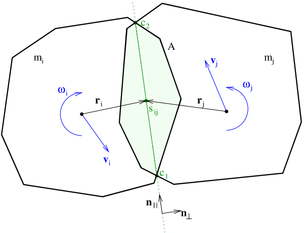
Figure 1: (Color online) Sketch of two polygonal particles in contact. The normal and tangential direction of a collision is determined by the contact line (green), the contact point is defined as the middle of the contact line.

$$m_{\parallel}=\frac{1}{\frac{1}{m_{i}}+\frac{1}{m_{j}}+\frac{r_{i}^{2}}{J_{i}}+\frac{r_{j}^{2}}{J_{j}}}$$ (31)

The relative tangential velocity at the contact point $s_{ij}$ is

$${v}_{\parallel}=(\bm{v}_{i}-\bm{v}_{j}+(\bm{r}_{i}\times\bm{\omega}_{i})-(\bm{r}_{j}\times\bm{\omega}_{j})\ )\cdot\bm{n}_{\parallel}.$$ (32)

where $\bm{v}_{i},\bm{v}_{j}$ are the velocities of the particles and $\bm{\omega}_{i},\bm{\omega}_{j}$ are their angular velocities. Furthermore, we define the effective penetration length as

$$h_{\text{eff}}=\frac{A}{l}\>.$$ (33)

Note that $l$ does not change significantly during a collision, so $h_{\text{eff}}$ is essentially proportional to the overlap area $A$. The normal component of the contact force is determined by the equation

$$F_{\perp}=\max\left[Eh_{\text{eff}}-\gamma\sqrt{Em_{\perp}}\dot{h}_{\text{eff}}~{};~{}0\right].$$ (34)

Here $E$ is the two-dimensional Young’s modulus and $\gamma$ is the dissipation strength.

The maximum function in (34) ensures that the normal force cannot become attractive. Physically, situations where the dissipative term overcomes the repulsive force correpond to the case that the particles’ separation velocity is faster than the relaxation velocity of the grain deformation, i.e., the contact between the particles is lost, before the overlap of the non-deformable model particles becomes zero Schwager and Poeschel (2007). Consequently, the contact force vanishes from this moment on.

We used the Cundall-Strack model Cundall and Strack (1979) for modelling tangential forces. At the beginning of the collision, the Cundall-Strack force $F^{*}$ is zero. If this force is given at the previous timestep, corresponding to time $t_{c}-\Delta t$, the Cundall-Strack force at the current timestep at time $t_{c}$ is determined by

$$F^{*}_{\parallel}(t_{c})=$$

$$\min\left[F^{*}_{\parallel}(t_{c}-\Delta t)+v_{\parallel}(t_{c}-\Delta t)\Delta t\frac{2}{7}E~{};~{}\mu F_{\perp}(t_{c})\right]\>.$$ (35)

One may visualize this model as a spring between the contact points being established when a new contact appears and the length of the spring being limited by the value of Coloumb friction (Coulomb condition). If this value is reached, the points of attachment of the spring start to slide, so that the spring length remains constant. In this way, the Cundal-Strack model mimics sticking and sliding friction. In order to avoid unrealistic oscillations, a damping term proportional to the velocity is added to the Cundall-Strack force, which also satisfies the Coloumb conditions. The complete trangential force then is

$$F_{\parallel}(t_{c})=\min\left[F^{*}_{\parallel}(t_{c})+v_{\parallel}\sqrt{\frac{2}{7}Em_{\parallel}}~{};~{}\mu F_{\perp}(t_{c})\right].$$ (36)

With (34) and (36), all the contact forces and the resulting torques between the particles and between particles and walls (which are treated as particles with fixed position and orientation) are defined. The equations of motion (27) and (28) are then solved numerically using a sixth-order Gear predictor-corrector method Gear (1967).

IV Excitation protocols and parameters

Inspired by former experimental studies Schröter et al. (2005); Zhao et al. (2012); Zhao and Schröter (2014), we implemented two protocols for exciting the granular matter periodically. In both protocols, an excitation period in which the phase space is explored alternates with a relaxation period in which the grains come to rest completely. Both protocols are characterized by a control parameter, which we call tapping parameter.

In all simulations, we used a bidisperse mixture of 1184 regular decagons, composed of 544 particles with radius $r_{1}=9\,\text{mm}$ and 640 particles with radius $r_{2}=6.36\,\text{mm}$. Young’s modulus was set to $E=1000\,\text{N}/\text{m}$ and the simulation time step was chosen as $\Delta t=5\cdot 10^{-5}\,\text{s}$. The Coulomb friction coefficent was taken to be $\mu=0.6$ and for the normal friction coefficent $\gamma=0.5$ was used. The particles mass density was $\rho=0.001\,\text{g}/\text{mm}^{2}$ and was the same for big and small particles.

With both protocols, the width of the simulation area was $280\,\text{mm}$. In the case of the negative $g$ protocol, there is no lid, for the rotating $g$ protocol the height of the box is $900\,\text{mm}$. Walls are realised as fixed rectangular particles with the same Young’s modulus and friction coefficients as the mobile particles.

Tejada et. al. Tejada and Jimenez (2014) pointed out that the size of the time step in DEM simulations may influence the width and the shape (but not the mean) of the determined probability distributions, even if the time step appears sufficiently small using common criteria. In order to make sure that this effect does not influence our results, we repeated some of the simulations with a time step of $\Delta t=10^{-5}\,\text{s}$. We found that the mean volume fraction, the volume fraction variance and also the shape of the volume fraction distribution did not change on reduction of the time step.

The first protocol, called “pulses of negative gravitation” or “negative g” protocol, is illustrated in figure 2a.

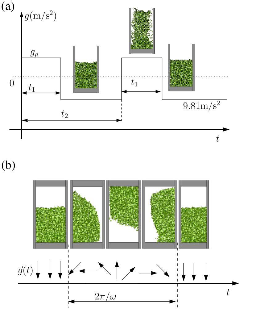
Figure 2: (Color online) a) The “negative g” protocol: For a short time interval $t_{1}$ the gravity is turned upward with a prescribed magnitude. Afterwards, the granular system has time to come to rest completely, before the next pulse starts. b) The “rotating g” protocol: The gravitational acceleration vector performs a complete rotation. Afterwards, the granular system comes to rest completely before the next round starts.

Most of the time, the granulate is at rest in a container under normal gravitation, but for short time intervals, the direction of gravitational acceleration is reversed. The time dependence of the gravitational acceleration $g(t)$ is taken to be

$$\bm{g}(t)=9.81~{}\text{m}/\text{s}^{2}\bm{e}_{y}\cdot\begin{cases}~{}g_{p}&\tilde{t}<t_{1}\\ -1&\text{otherwise}\end{cases}\>.$$ (37)

Here $\tilde{t}=t\bmod T$ is the simulation time $t$ modulus the period $T$ of the protocol and $t_{1}$ is the duration of a pulse. We took the pulse length to be $t_{1}=0.1\,$s and the period $T=3\,$s. The relaxation period was chosen so that for the biggest excitation amplitudes the resulting volume fraction variations due to remaining kinetic energy in the system are smaller than $10^{-5}$ which is 100 times smaller than the typical magnitude of the observed static volume fraction fluctuations. The pulse amplitude $g_{p}$ was used as a tapping parameter. Due to Einstein’s equivalence principle, this protocol is equivalent, per period, to a downward acceleration $(g_{p}+1)g$ for an interval $t_{1}$ and a subsequent stoppage in the gravitational field for a time span $T-t_{1}$, taken long enough for the granulate to come to rest. Here and in the following when we write $g$, we mean $g=9.81\,\text{m/s}^{2}$.

Figure 2b illustrates the second protocol. The granulate is at rest in a closed box. Then the gravitational acceleration performs a complete rotation followed by a relaxation period.

$$\bm{g}(t)=9.81\text{m}/\text{s}^{2}\cdot\begin{cases}\sin(\omega t)\bm{e}_{x}-\cos(\omega t)\bm{e}_{y}&\tilde{t}<\frac{\omega}{2\pi}\\ -\bm{e_{y}}&\text{otherwise}\end{cases}\>.$$ (38)

As in the negative g case, $\tilde{t}=t\bmod T$ is the simulation time $t$ modulus the period $T$. The angular frequency $\omega$ is the control parameter of the protocol. Of course $T>2\pi/\omega$ must be fulfilled. In our simulations, we used $T=2\pi/\omega+3\,$s, with $\omega\gtrsim 4\,\text{s}^{-1}$. For both protocols, we tested whether or not segregation of the particles occurs by measuring the cumulative number of small and big grains as function of the column height $n(h)$ (i.e. the number of small or big particles with $z$ coordinates smaller than $h$). These curves are straight lines and do not change during the simulations, except for fluctuations. Therefore we conclude that in our simulations segregation did not take place.

V Determination of compactivity, fluctuations and the partition function

For both protocols and each choice of the tapping parameter the simulations ran for $2500-3000$ excitation and relaxation periods. Note that this relatively high number of taps is necessary to draw serious conclusions for the systems used here. While the confidence interval of the mean volume fraction became sufficiently small after some hundred taps, this was not the case for the estimated variance. In test simulations, where only a few hundred taps were considered, the uncertainty of the estimated variance (Bronstein et al., 1999, pp. 771–772) was as big as the domain of the measured variance itself.

Immediately before the relaxation period ended, we determined the volume fraction of the granulate by measuring the fraction of solid particles in a test volume. The test volume shown in figure 3 is a square with edge length of $400\,\text{mm}$ and was chosen in such a way that some layers of particles were between the borders of the test region and the walls.

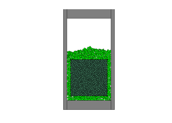
Figure 3: (Color online) A typical situation when the granulate is at rest. The region shaded grey is the test volume, used for volume fraction determination.

It was pointed out Gago et al. (2015) that test volumes must be big enough to avoid size depended effects. To make sure that our test volume is sufficiently large, we divided it into two neighbouring columns. The relative difference of mean volume fraction (after 2500 taps) between the columns and the entire test volume was always smaller than $0.01\,$% and the deviation of the volume fraction fluctuation ratio from $\sqrt{2}$ was always lower than $1\,\%$.

Figure 4 shows some typical time series for both protocols. The mean volume fraction reaches a steady state value very quickly (after approximately $<10$ taps) and then only fluctuations around its mean value occur.

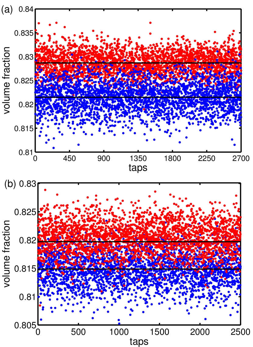
Figure 4: (Color online) Exemplary time series for both protocols. The points are the volume fractions calculated from simulation data and the solid lines are the corresponding mean values. The tapping parameter is for the “negative $g$” protocol (a): $g_{p}g=6\text{m/s}^{2}$ (red points) and $g_{p}g=28\text{m/s}^{2}$ (blue points) and for the “rotating $g$” protocol $\omega=0.75\cdot 2\pi~{}\mathrm{s}^{-1}$ (red points) and $\omega=2\cdot 2\pi~{}\mathrm{s}^{-1}$ (blue points).

In Fig. 5, the mean value of the volume fraction $\bar{\phi}$ and the standard deviation of the volume fraction distribution, characterizing the volume fraction fluctuation strength, are shown. Initially, the volume fraction decreases with increasing pulse strength until it reaches a local minimum around $g_{p}=20$. Afterwards, the volume fraction increases with the pulse strength. Similar behaviour for tapped granulates at high tapping strengths was described in Gago et al. (2009); Pugnaloni et al. (2010). A possible explanation is the interplay between two competing effects. First, the stronger the pulse of negative gravitation, the more the granulate is whirled around, i.e. the looser the resulting packing should get. On the other hand, the stronger the pulse, the higher the granulate flies, therefore the higher its impact velocity when it reaches the bottom, resulting in stronger compaction during the relaxation period. The first effect dominates for relatively small values of $g_{p}$, the second effect becomes more important for stronger pulses. At the same value of $g_{p}$, where the volume fraction is minimal, the volume fraction fluctuations have a local maximum (see Fig. 5b). Similar results were found in work by Pugnaloni et al. Pugnaloni et al. (2010).

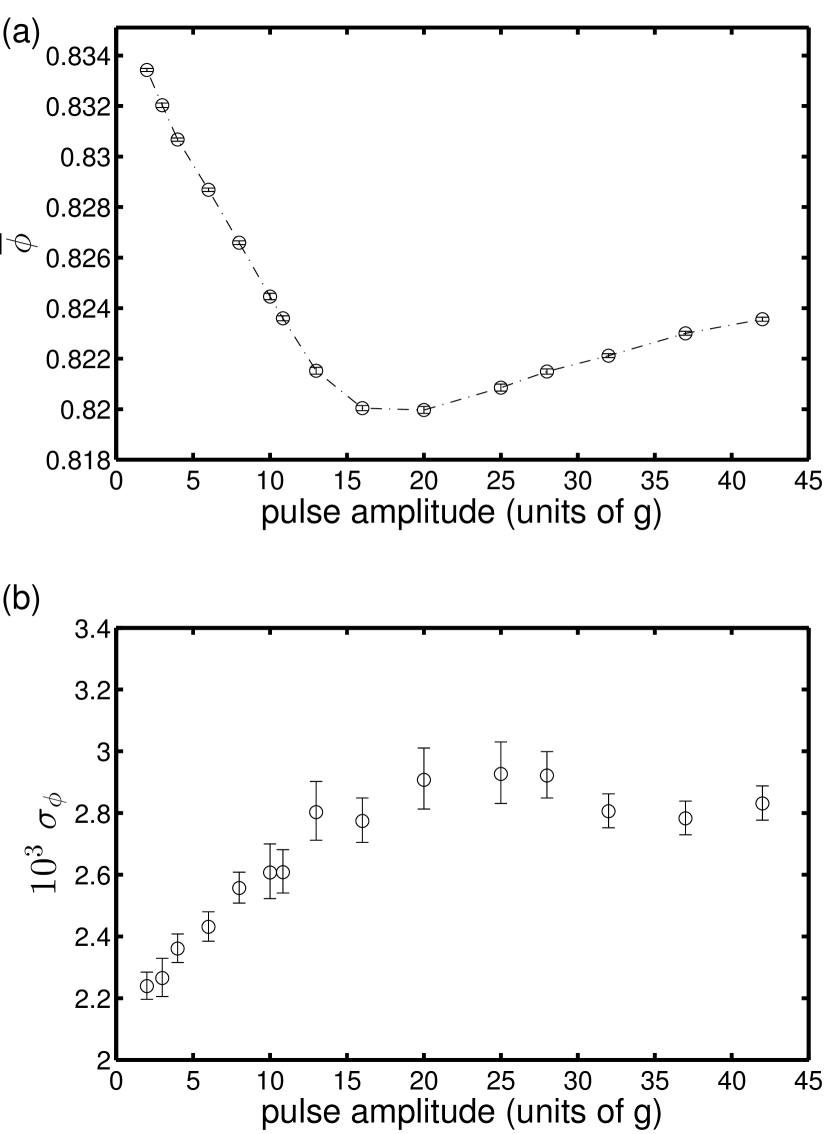
Figure 5: Simulation results for the “negative g” protocol: (a) the mean volume fraction as function of the pulse strength in units of earth acceleration is depicted, (b) shows the standard deviation of the volume fraction fluctuations. The error bars correspond to a confidence interval of 95 percent.

The corresponding results for the “rotating g” protocol are shown in figure 6. With increasing frequency the mean volume fraction shows a crossover from $\bar{\phi}\simeq 0.814$ to $\bar{\phi}\simeq 0.821$. When the frequency is very small, a complete rotation takes a long time and the granulate behaves in a quasistatic way. It is clear that in this case a further decrease of the frequency will not have a significant influence on the resulting volume fraction. Therefore, for small frequencys the $\phi(\omega)$ curve should approach a plateau. When the frequency increases, the rotation gets faster, the granulate is more strongly whirled around and becomes looser. When the frequency increases further, the time per rotation gets smaller which compensates the increase of swirling due to faster rotation. For very high frequency, one expects that the system reaches an irreversible regime, because it does not have time to respond to the rotation pulse and will largely stay in the initial configuration - but this regime is not reached in our simulations.

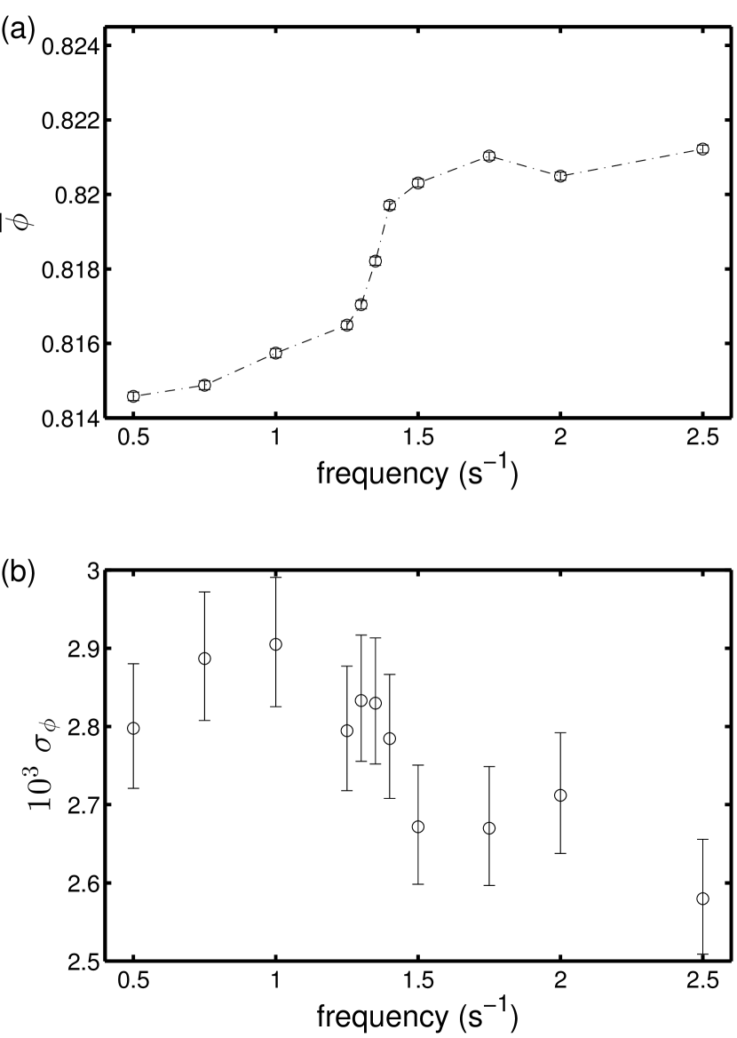
Figure 6: Simulation results for the “rotating g” protocol: Part (a) shows the mean volume fraction as function of rotation frequency $f=\omega/(2\pi)$ and (b) shows the standard derivation of the volume fraction fluctuations. The errorbars correspond to a confidence interval of $95$ percent.

In order to determine the granular temperature of the samples with the overlapping histogram method, the probability density distribution of the volume fraction must be estimated. Notwithstanding the name of the approach, we used the more sophisticated kernel density estimation method Rosenblatt (1956); Parzen (1962) instead of histograms in order to obtain an approximation for the probability density. A normal kernel was employed and the bandwidth was chosen according to Silverman’s rule of thumb Silverman (1998). In appendix B, a short description of the approach is offered.

Some of the determined probability density distributions are shown in Fig. 7a for the “negative g” protocol and in Fig. 8a for the “rotating $g$” protocol. In order to test if the distributions are Gaussian, we used a chi-square test Bronstein et al. (1999) with a significance level of $5$%. The null hypothesis that the data is normally distributed was rejected for all samples . Although Gaussians may still be good approximations to the central region of our distributions, we take this as evidence for a statistical mechanical origin of these distributions rather than their emergence from some unknown additive process not related to phase space exploration. Therefore, we believe that our data do not give spurious results due to the pitfall described in appendix A.

We also show in appendix A that while the presence of Gaussian distributions may lead to false positive results regarding the validity of Edwards’ theory McNamara et al. (2009), this is by no means true for all Gaussian distributions: in the limit of large numbers, the canonical distribution corresponding to a fixed compactivity must become Gaussian as well, and this distribution obviously satisfies Edwards’ theory by definition. We take the fact that the tails of our distributions are non-Gaussian together with the verification of (20) as an indication that the theory works. This interpretation is supported by other studies of very similar systems where the volume-per-particle distribution (which is not a sum and therefore not subject to the central limit theorem) was found not to be Gaussian Zhao and Schröter (2014); McNamara et al. (2009) even in the central region.

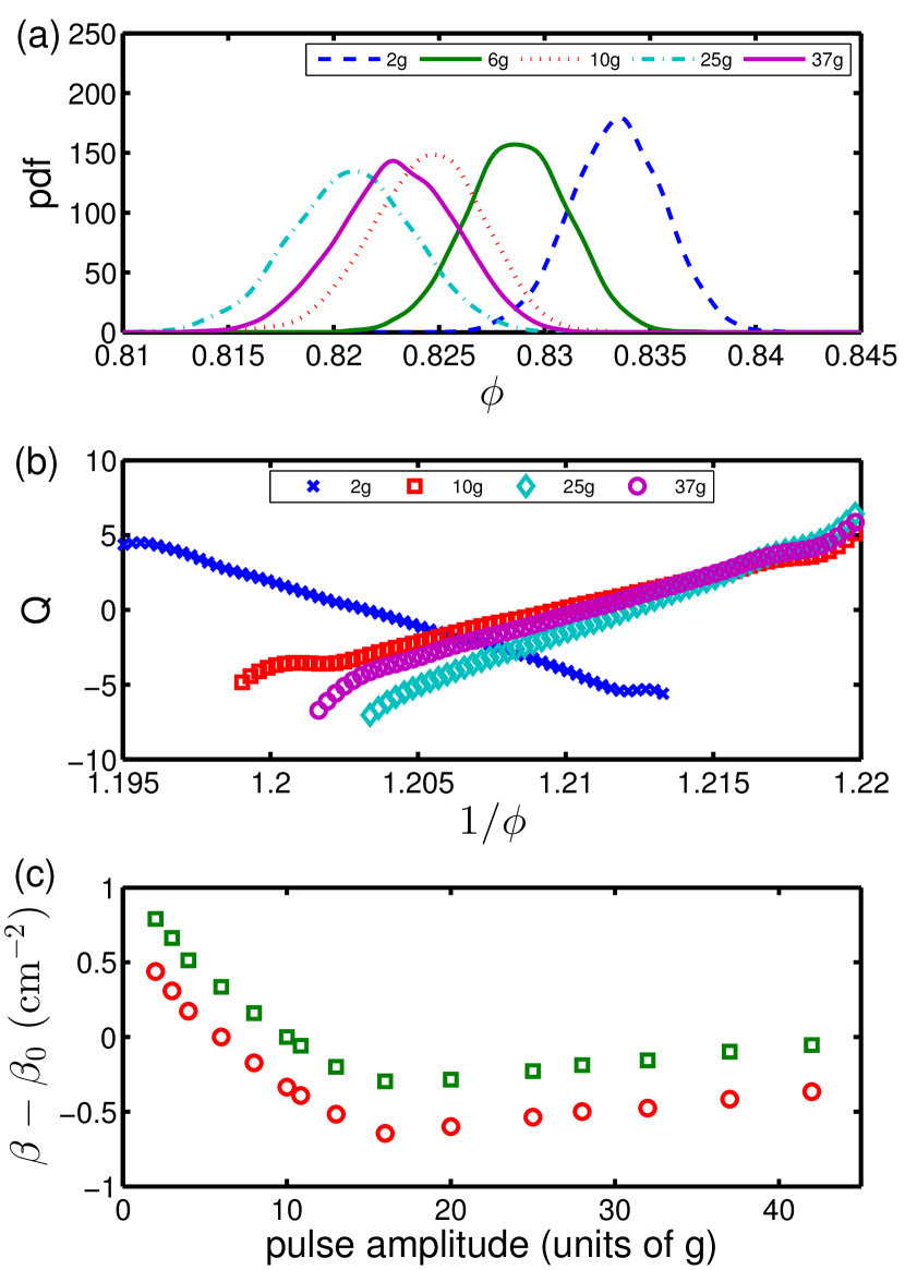
Figure 7: (Color online) (a) Probability density function of the volume fraction for the “negative g” protocol, estimated with the kernel density method, for different values of the pulse strength. (b) The quantity $Q$ from equation (20) for some values of the tapping parameter, where the distribution with $g_{p}=6$ was chosen as denominator in (19). (c) The compactivity calculated with the help of the overlapping histogram method using the distribution with $g_{p}=6$ (green, squares) and $g_{p}=10$ (red, circles) as denominator in (19).

In terms of volume fraction, equation (20) reads:

$$Q =\ln\frac{P(\phi,\beta_{1})}{P(\phi,\beta_{0})}$$

$$=-(\beta_{1}-\beta_{0})\frac{V_{g}}{\phi}-\ln\frac{Z(\beta_{1})}{Z(\beta_{0})}.$$ (39)

We note that (39) is interpreted in terms of a canonical ensemble, which implies the number of particles to be a constant. This means that the total volume of the grains $V_{g}$ in the test volume must be a constant . In principle, one would have to adapt the test volume size $V_{T}$ used in determining the volume fraction distribution to the measured mean volume fraction $\bar{\phi}$ in such a way that $V_{g}=V_{T}\,\bar{\phi}$ remains constant. The size of the test volume would then be a function of the mean volume fraction. This could become important, if very small test volumes were used. The standard deviation of the volume fraction distribution should decrease with increasing test volume as $\sigma\propto V^{-1/2}$, which follows from (17), while $\bar{\phi}$ does not depend on the system size. By using a constant test volume $V_{T}$, the magnitude of differences in $V_{g}$ due to different volume fractions is bounded by $\Delta V_{g}=V_{T}(1/\phi_{\text{rcp}}-1/\phi_{\text{rlp}})\simeq 0.05V_{T}$. If the test volume is large compared to the size of the particles, the relative error which is made by using a constant test volume, assuming that the cumulative grain volume is constant (in spite of the different volume fractions), corresponds to approximately $(2-3)\%$. This is smaller than the confidence interval of $\sigma_{\phi}$ due to the finite sample size and therefore negligible.

By choosing a reference probability distribution which is used as the denominator in (39) we are able to determine the inverse compactivity and the logarithm of the partition function up to additive constants, which are the unknown inverse compactivity of the reference distribution and the unknown logarithm of the partition function thereof, respectively. In order to avoid errors due to insufficient data in the tails of the distribution, we evaluated the slope of $Q$ only in regions where the value of each distribution involved in the calculation of (39) is bigger than $5$% of its maximum.

Figures 7b and 8b show the quantity $Q$ for some samples as function of the inverse volume fraction, where the distribution with $g_{p}=6$ of the “negative g” protocol was chosen as the reference distribution, because it has sufficient overlap with all the other distributions. We tried several other distributions as references, too. So long as the distribution overlap was big enough, we always found a linear relation between $Q$ and the inverse volume fraction $\phi^{-1}$. This may be interpreted as suggestive of the validity of Edwards’ assumptions. Note that the deviations from the straight line on the left and right ends of the curves are due to insufficient number of sampling data points in that region. Therefore the estimated probability density function behaves like the tails of the sampling kernel, which is reflected also in $Q$. This behaviour is a mathematical artefact and not a systematic deviation from a straight line.

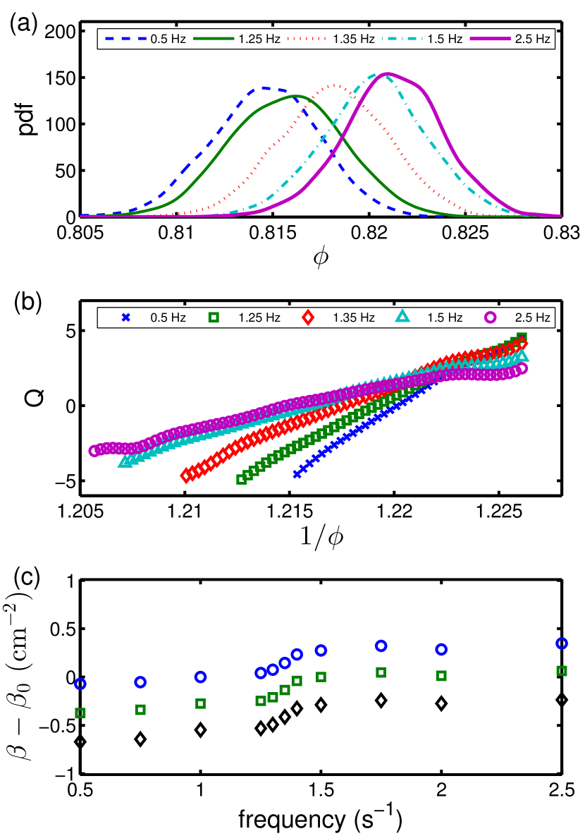
Figure 8: (Color online) (a) Probability density function of the volume fraction for samples of the “rotating g” protocol, estimated with the kernel density method, for different values of the rotation frequency. (b) The quantity $Q$ from equation (20) for some values of the tapping parameter using the distribution with $g_{p}=6$ of the “negative g” protocol as denominator in (19). (c) The compactivity calculated with the help of the overlapping histogram method using the distribution from the “rotating g“ protocol with $f=0.5Hz$ (blue, circles), $f=1.25Hz$ (green, squares) and the distribution from the “negative g” protocol with $g_{p}=6$ (black, diamonds) as denominator.

From (39), it follows immediately that the values determined for $\beta$ using different samples as reference distribution may only differ by an additive constant. This prediction holds for the “negative g” protocol as is demonstrated in Figure 7c. There, the samples with $g_{p}=6$ and $g_{p}=10$ were used as reference distributions. The same is true for the “rotating g” protocol (Fig. 8c) when we used samples corresponding to different values of the rotating frequency. It even applies if we use samples from the “negative g” protocol as reference distribution, in agreement with the fact that the predictions of Edwards’ theory should be protocol independent.

From now on, we use the distribution from the “negative g” protocol with $g_{p}=6$ as reference distribution for all the following calculations. Figure 9 shows the values determined for the inverse compactivity for both protocols as function of the volume fraction. All the data, whether obtained from the branch left of the minimum or the branch right of the minimum in the $\phi(g_{p})$ curve of the “negative g” protocol (cf. Fig. 5) or else from the “rotating g” protocol is fitted by the same function $\beta(\phi)$. This is a strong indicator for the applicability of Edwards’ theory to our samples.

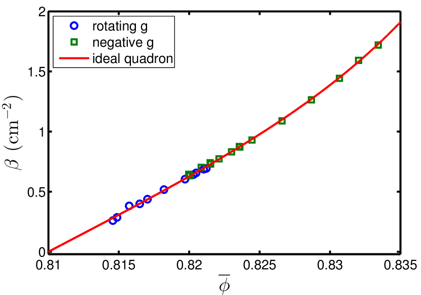
Figure 9: (Color online) The compactivity as function of the volume fraction density for the “negative g” protocol (square) and for the “rotating g” protocol(diamonds). The values were corrected with the additive constant $\beta_{0}$ determined from the ideal quadron fit. The solid line is a fit to the ideal quadron solution (26)

.

In order to fit our results to an analytical function, we used the ideal quadron solution (26). The values of random loose packing (rlp) and random close packing (rcp) were assumed to be $\phi_{\text{rlp}}=0.81$ and $\phi_{\text{rcp}}=0.855$. The choice of these values was pragmatic. To our knowledge, there are no studies about the exact values for random close and random loose packing for bidisperse decagons. Furthermore the values of rlp and rcp will depend on on the size ratio between the particles. Therefore, we used plausible values obtained for (bidiperse) disks Berryman (1983); Silbert (2010); Zhao and Schröter (2014). We checked that the influence of the values of random loose and random close packings on the values of the obtained parameters are smaller than $20\,\%$, as long as the values are in the plausible interval.

$N\bar{z}/V_{g}$ was used as fitting parameter. Since we can determine the inverse compactivity only up to an additive constant from the overlapping histogram method, we made the replacement $\beta\rightarrow\tilde{\beta}+\beta_{0}$ in (26), where $\tilde{\beta}$ is the value determined from the simulations and $\beta_{0}$ is taken as an additional fit parameter. Note that the determination of $\beta_{0}$ is possible as we assumed that the inverse compactivity is fixed at random loose and random close packing and that this is not specific to the ideal quadron fit. We emphasize that the parameter $\beta_{0}$ only shifts the whole curve shown in Fig. 9 upward or downward and is the same for both protocols. Since the same value of $\beta_{0}$ was added to every data point obtained from the overlapping histogram method for the comparison of the fit function with the simulation data in Fig. 9, this value does not influence the conclusion that the compactivity is the same for both protocols. The fit describes the simulation data very well, as is seen in Fig. 9. However, we find as fitting value $N\bar{z}/V_{g}=556.51\,\text{m}^{-2}$, which differs by about a factor of $40$ from the values used in the simulation. This might be understood by assuming that approximately 40 quadrons constitute a statistically independent unit in the granular ensemble. This issue certainly needs further study. We also tried to fit $\phi_{\text{rlp}}$ and $\phi_{\text{rcp}}$ and using the known particle number in (26) but this leads to an unphysical value for random close packing of about $\phi_{\text{rcp}}\simeq 1.2$.

When we used only the data obtained by one of the protocols to determine the parameters of the ideal quadron solution, the solution fitted the data of the other protocol. The relative deviation of the obtained fitting parameters is smaller the $2\,\%$. Because this results in curves that are indistinguishable to the eye, only the fit using the whole dataset is presented in in Fig. 9. Nevertheless, this means that we can predict the $\beta(\phi)$ curve, for the “rotating $g$” protocol using the data determined from the “negative $g$” protocol and vice versa. However, for all compactivities determined, the same reference distribution was used so the data of the fit employed for the one and the other protocol was not entirely independent.

While the slope of $Q$ allows us to determine the inverse compactivity, the axis intercept $B$ determines the logarithm of the partition function

$$B=-\ln Z(\beta)+\ln Z(\beta_{0}).$$ (40)

If the assumptions leading to (39) are correct, the partition function of the ideal quadron solution (21) should describe the found intercept without additional fitting. The parameters $\Delta$, $V_{0}$, $Nz$ are directly related to the parameters determined via Eqs. (24) and (25). As Fig. 10 shows, the numerically determined values and the ideal quadron solution fit very well, independently of the protocol and of the branch in the “negative g” protocol.

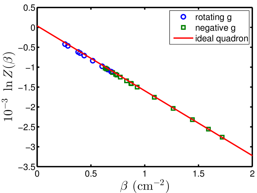
Figure 10: (Color online) The logarithm of the partition function, determined from the overlapping histogram method(symbols). The solid line is the ideal quadron solution.

Using (26) in (17), we get the relationship between the mean volume fraction and its fluctuations. The result together with simulation data obtained directly is shown in figure 11. The data is in good agreement with the theory for both protocols.

We mention that in a former study which used vertically tapped monodisperse regular polygons Carlevaro and Pugnaloni (2011), a maximum in the $\phi-\sigma$ curve was reported which coincided with an inflexion point in the impulse strength - volume fraction curve. In our simulation we do not see this effect, also in experimental work about bidisperse two dimensional systems such a maximum was not observed Zhao and Schröter (2014). It might be speculated that crystallization effects that occur frequently in two-dimensional monodisperse systems were responsible for the occurrence of the maximum in Ref. Carlevaro and Pugnaloni (2011), but this question cannot be clarified in this study.

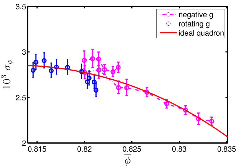
Figure 11: (Color online) The volume fraction fluctuation (standard deviation) as function of the mean volume fraction. The blue points correspond to the “rotating g“ protocol and the magenta points and lines corresponds to the negative g” protocol. The solid line is the ideal quadron fit.

However, we cannot exclude that there may be a small hysteresis for the branch pieces to the left of minimum and to the right of minimum, respectively (cf. Fig. 5). Clearly, if the volume ensemble completely described all structural degrees of freedom and the probability, two states with the same $\beta$ and the same $\phi$ would be identical and therefore $\sigma_{\phi}$ would also have to be the same. However, if the volume ensemble is only a good approximation of the geometric aspects of interdependent force-moment and volume ensembles (see, e.g. Blumenfeld et al. (2012)), deviations may occur.

VI Limitations of the volume ensemble

Whereas the volume ensemble appears to succeed in describing the geometrical and structural degrees of freedom of a granular aggregate, this is not the case for the stress state of the latter. If the volume ensemble entailed a complete description of a granular state and its probability distribution, the mean stress of the system would have to be a unique function of the inverse compactivity and therefore also a unique function of the mean volume fraction. We computed the mean extensive stress (or force-moment tensor), defined as

$$\bm{S}_{ij}=\sum_{p}V^{p}\sigma^{p}_{ij}$$ (41)

as a function of the volume fraction. Note that the volume density of this tensor is the stress itself. Here $i$ and $j$ label Cartesian coordinates. The sum runs over all particles, where $\sigma_{ij}^{p}$ is the mean stress in particle $p$ and $V^{p}$ is the volume associated with the particle. The result is shown in Fig. 12. The stress tensor is obviously not a unique function of the volume fraction.

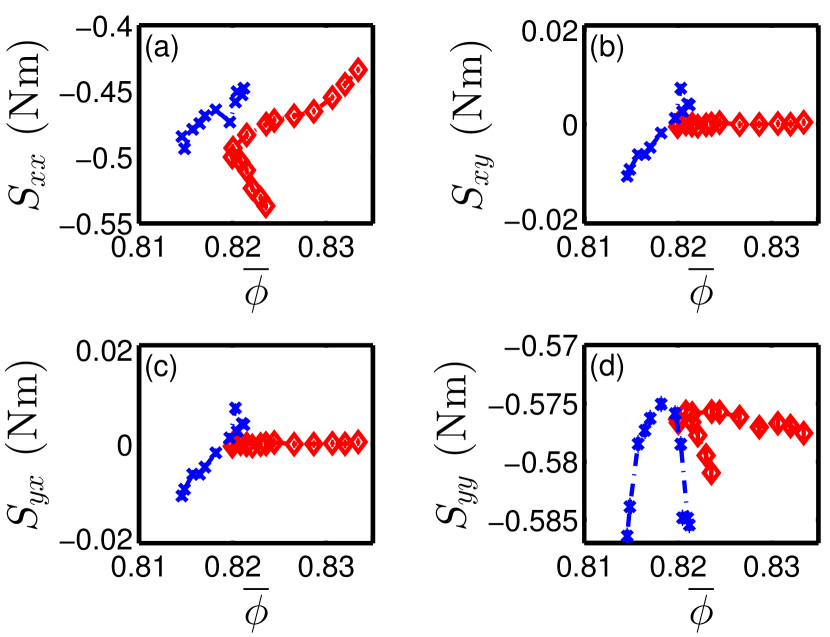
Figure 12: (Color online) The components of the extensive stress tensor as function of the mean volume fraction for the “negative g” protocol (diamonds) and the “rotating g” protocol (crosses).

Neither the results from the different protocols nor the results from the half-branches left to the minimum and right to the minimum, respectively, of the “negative g” protocol fall on the same curve, which is in agreement with similar findings on tapped granular matter Pugnaloni et al. (2010). Two systems with almost identical particle positions and orientations can be in very different stress states which is not captured by the volume ensemble. To describe the stress state and the volume state together, probably the combined volume-stress ensemble Blumenfeld et al. (2012) must be taken into account. We remark that it is unclear so far wether or not the stress states observed here are “very different” or even “very similar” because we do not know the size of the accessible phase space for the extensive stress tensor. Maybe the deviations in our systems which have magnitude on the order of $0.01\,\text{Nm}$ are so small that it is reasonable to assume in first approximation that the stress-moment tensor is almost constant which would be a possible explanation for the success of assuming a pure volume ensemble.

VII Conclusions

We used two different protocols to excite a granular ensemble periodically. The inverse compactivity was determined as a function of the mean volume fraction and we found that the relation between the compactivity and the mean volume fraction is protocol independent. We determined an expression for the logarithm of the partition function and thus the thermodynamic potential which is the equivalent of the free energy of classical statistics. This was done by using the ideal quadron solution derived by Blumenfeld and Edwards Blumenfeld and Edwards (2003) as a fitting function. Even though the ideal quadron solution makes very rough assumptions, the resulting description is in qualitative agreement with the findings from the simulations. If the particle number is used as a fit parameter instead of calculating the distribution with the true particle number, the ideal quadron solution is also able to describe the results quantitatively.

We found that all our simulation results related to structural quantities are compatible with Edwards’ theory and that the Edwards theory describes the volume fluctuations very well, independently of the excitation protocol. The usage of the Edwards volume ensemble seems to be sufficient for the description of system properties which are related to the geometrical arrangement of the grains, but as might be expected from previous findings, it is not sufficient to describe the stress states of the granular ensemble.

Appendix A Overlapping histograms for Gaussian distributions

If two volume samples were Gaussian distributed with mean values $V_{1}$ and $V_{2}$ and variances $\sigma_{1}^{2}$ and $\sigma_{2}^{2}$, the corresponding $Q$-function defined in (19) would be McNamara et al. (2009):

$$Q^{g}(V)=-\frac{(V-V_{1})^{2}}{2\sigma_{1}^{2}}+\frac{(V-V_{2})^{2}}{2\sigma_{2}^{2}}+\ln\left(\frac{\sigma_{2}}{\sigma_{1}}\right).$$ (42)

This is a quadratic function of $V$, but in some $V$ interval the curvature of $Q^{g}$ may be very small and the parabolic function (42) would then practically be indistinguishable from a linear function. This happens in particular, if the variances $\sigma_{1}$ and $\sigma_{2}$ are close to each other, i.e., for nearby compactivities. If we define a function $A^{g}_{21}$ as the slope of (42) midway between the maximum values of the two normal distributions,

$$A^{g}_{21}:=\left.\frac{\mathrm{d}}{\mathrm{d}V}Q^{g}(V)\right|_{V=(V_{1}+V_{2})/2}\>,$$ (43)

we obtain McNamara et al. (2009):

$$A^{g}_{21}=\frac{1}{2}\left(\frac{1}{\sigma_{1}^{2}}+\frac{1}{\sigma_{2}^{2}}\right)\left(V_{1}-V_{2}\right).$$ (44)

Identifying formally

$$A^{g}_{21}=\beta(V_{2})-\beta(V_{1})\>,$$ (45)

we find from (44):

$$-\frac{V_{2}-V_{1}}{\beta(V_{2})-\beta(V_{1})}=2\left(\frac{1}{\sigma_{1}^{2}}+\frac{1}{\sigma_{2}^{2}}\right)^{-1}\>.$$ (46)

If we assume that the variance is a unique function of the mean volume, this equation is an approximation of (12) which is the better the smaller the difference $|V_{2}-V_{1}|$.

We note that the formal identification (45) is strictly speaking inherently contradictory, which is easy to see if we calculate $Q$ for a third sample with mean value $V_{3}$ and variance $\sigma_{3}$ and the same reference sample in the denominator. From (45) $A_{31}-A_{21}=A_{32}$ follows, but if one calculates the same quantity from (44), the result does not agree. (However, the identification is possible, if the three variances are the same.)

Analogously, we can calculate the intercept $B^{g}_{21}$ of the tangent which touches (42) at $V=(V1+V2)/2$:

$$B^{g}_{21} =\frac{1}{8}(V_{2}-V_{1})^{2}\left(\frac{1}{\sigma_{2}^{2}}-\frac{1}{\sigma_{1}^{2}}\right)+\ln\left(\frac{\sigma_{2}}{\sigma_{1}}\right)$$

$$\>\>+\frac{1}{4}\left(V_{2}^{2}-V_{1}^{2}\right)\left(\frac{1}{\sigma_{1}^{2}}+\frac{1}{\sigma_{2}^{2}}\right)\>.$$ (47)

By calculating the limit

$$\lim_{V_{2}\rightarrow V_{1}}\frac{B^{g}_{21}}{A^{g}_{21}}=-{V}_{1}-\sigma_{1}\frac{\partial\sigma_{1}}{\partial V_{1}}$$ (48)

we find that the term $B^{g}_{21}/A^{g}_{21}$ is an approximation for (10), if we assume $\frac{\partial\sigma_{1}}{\partial V_{1}}$ to be negligibly small and formally identify $B_{21}^{g}=\ln(Z_{2})-\ln(Z_{1})$. Again the approximation becomes better as the difference between the volume $V_{2}$ and the reference volume $V_{1}$ gets smaller.

Due to these similarities, it might occur that even if the relations (10), (12) and (20) are consistent, that within the limits of data precision it is not possible to decide whether the reason of this agreement is the correctness of Edwards’ theory or the fact that the data generated by a specific protocol happen to have a distribution that is well approximated by a normal distribution. If the samples are generated using the same protocol, one may expect that there is a function $\sigma(V)$, but when different protocols are used, it would be surprising, if both protocols led to the same relation, unless a general principle, such as Edwards’ theory, were at work.

On one hand, these similarities make it more difficult to verify Edwards’ theory, on the other hand, due to the central limit theorem, we should expect that the distribution of Eq. (18) becomes more and more Gaussian with increasing system size. Therefore, it is not always true that the appearance of Gaussian distributions signifies inapplicability of the overlapping histogram method in the determination of the compactivity and of related quantities. Let us briefly have a look at this. Rewriting Eq. (18) for general $\beta$ and using the microcanonical result for the density of states, we have

$$P(V,\beta,N) =\frac{\Omega(V,N)}{Z(\beta,N)}e^{-\beta V}=\frac{e^{S(V,N)-\beta V}}{Z(\beta,N)}\>.$$ (49)

As in standard statistical mechanics, we can then argue that for large systems this distribution has a sharp peak at the mean value of the volume and we may expand the entropy about this average, neglecting terms that are of higher than quadratic order:

$$S(V,N)-\beta V \approx S(\bar{V},N)+\beta(\bar{V})\left(V-\bar{V}\right)$$

$$\>\>+\frac{1}{2}\frac{\partial^{2}S}{\partial V^{2}}\Big{|}_{\bar{V}}\left(V-\bar{V}\right)^{2}-\beta V\>.$$ (50)

In order for the expansion to be about the maximum of the distribution, we must require the linear order term to vanish, i.e., we have $\beta(\bar{V})=\beta$, meaning equivalence of the microcanonical and the canonical compactivity definitions. Identifying the inverse of $-\partial^{2}S/\partial V^{2}$ with the variance, our distribution takes the form

$$P(V,\beta,N) =\frac{e^{S(\bar{V},N)-\beta\bar{V}-\left(V-\bar{V}\right)^{2}/2\sigma^{2}}}{Z(\beta,N)}\>.$$ (51)

Evaluating this at two different compactivities and taking the logarithm of the ratio, we find (denoting the mean volumes by $V_{1}$ and $V_{2}$ again)

$$Q(V) =\ln\frac{P(V,\beta_{1},N)}{P(V,\beta_{2},N)}=-\frac{(V-V_{1})^{2}}{2\sigma_{1}^{2}}+\frac{(V-V_{2})^{2}}{2\sigma_{2}^{2}}$$

$$\>\>-\beta_{1}V_{1}+S(V_{1},N)+\beta_{2}V_{2}-S(V_{2},N)$$

$$\>\>+\ln\frac{Z(\beta_{2},N)}{Z(\beta_{1},N)}\>,$$ (52)

which is nothing but (42) with an explicit expression for $\ln(\sigma_{2}/\sigma_{1})$. But we have derived this as an approximation to the distribution (18) from which we obtain Eq. (20) for $Q$. If we substitute $\beta_{2}$ for $\beta_{0}$ in that equation, we see that the following (non-trivial) approximation holds in sufficiently large systems (close to the “thermodynamic limit”), as long as the distributions overlap significantly (which of course becomes less likely with increasing system size):

$$-(\beta_{1}-\beta_{2})V\approx-\frac{(V-V_{1})^{2}}{2\sigma_{1}^{2}}+\frac{(V-V_{2})^{2}}{2\sigma_{2}^{2}}$$

$$\>\>-\beta_{1}V_{1}+S(V_{1},N)+\beta_{2}V_{2}-S(V_{2},N)\>.$$ (53)

Hence, the sum on the right-hand side that is quadratic in $V$ is a good approximation to the sum on the left-hand side that is linear in $V$. As we have shown by this small calculation, the overlapping-histogram method will give, for such a system, the correct linear dependence on $V$, despite the fact that the central part of the distribution is well approximated by a Gaussian. In simulations, this behavior might be distinguished from Gaussian distributions not having the statistical mechanical origin postulated by the Edwards theory through verification that the tails of the simulated distributions, i.e., their behavior for $V$ values, where the quadratic approximation (50) breaks down, are not Gaussian. This was done for our simulations via the chi-square test mentioned in Sec. V.

Appendix B Kernel density estimation

A method to determine a continuous probability density from a data sample is the kernel density estimation method (KDE) Parzen (1962); Rosenblatt (1956). If $x_{1},x_{2},...,x_{n}$ are sampled data, the kernel density estimation of the probability density $P(x)$ at the point $x$ is defined as

$$P(x)=\frac{1}{nh}\sum_{i=1}^{n}K\left(\frac{x-x_{i}}{h}\right)\>,$$ (54)

where $K(x)$ is the kernel which must be a non negative function that satisfies

$$\int_{-\infty}^{\infty}\text{d}x~{}K(x)=1\>.$$ (55)

and $h$ is a smoothing parameter called the bandwidth. Possible kernels are for example the normal kernel

$$K(x)=\frac{1}{2\pi}\exp(-x^{2}/2)\>,$$ (56)

the Cauchy kernel

$$K=\frac{1}{\pi(1+x^{2})}\>,$$ (57)

the Epanechnikov kernel

$$K(t)=\begin{cases}\frac{3}{4}(1-x^{2})&\text{if}~{}x\in[-1;1]\\ 0&\text{elsewhere}\end{cases}\>,$$ (58)

or even the rectangular kernel:

$$K(t)=\begin{cases}1&\text{if}~{}x\in[-1/2;1/2]\\ 0&\text{elsewhere}\end{cases}\>.$$ (59)

The latter is equivalent to a histogram with bin width $h$. While it can be shown that the Epanechnikov kernel is optimal in the sense that it minimizes the mean squared error between the estimated and the real probability distributions, we used a normal kernel since it allows to make a good estimation of the optimal bandwidth $h$. In general, the optimal bandwidth can only be calculated if one knows the underlying probability density, but this density is unknown. In practice, therefore, Silverman’s rule of thumb is commonly used. Under the assumption that the underlying probability distribution is Gaussian and if a Gaussian kernel is used, the optimal bandwidth is

$$\left(\frac{4\sigma^{5}}{3n}\right)^{\frac{1}{5}}\simeq 1.06\sigma n^{-1/5}\>,$$ (60)

where $\sigma$ is the standard derivation of the sample. It turns out that this bandwidth is also a reasonable choice in practical situations, if the underlying distribution is not Gaussian. We note that for small data sets the choice of the kernel may have a significant influence on the quality of the fit. However, if the data sample becomes big enough, all kernels leads to almost the same results except for the far tail of the distribution, where no data points are available. In this region, the kernel itself specifies the decay of the distribution. As it is shown exemplarily in Figure 13, the choice of the kernel is not crucial for our data samples. The results obtained with the optimal Epanechnikov Kernel and the results achieved with the normal kernel are practically indistinguishable. The box kernel which is equivalent to a shifted histogram is a little bit more more irregular. We preferred the normal kernel, in order to avoid an ad hoc choice of the kernel bandwidth.

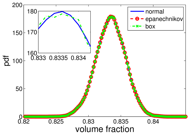
Figure 13: (Color onlie) Comparison of the results of kernel density estimation using different kernels. The shown data was obtained from the volume fraction time series of the “negative g” protocol with the tapping parameter $g_{p}=8$, for other parameters we found the same conclusion. The results due to the Epanechnikov kernel and the normal kernel are indistinguishable, the box kernel results in a little bit more irregular estimations. The inset shows the normal and the box kernel in the central region of the distribution.

References

- Edwards and Oakeshott (1989a) S. F. Edwards and R. Oakeshott, Physica A 157, 1080 (1989a).
- Edwards and Oakeshott (1989b) S. F. Edwards and R. Oakeshott, Physica D 38, 86 (1989b).
- Bi et al. (2015) D. P. Bi, S. Henkes, K. E. Daniels, and B. Chakraborty, Annual Review of Condensed Matter Physics, Vol 6 6, 63 (2015).
- Henkes et al. (2007) S. Henkes, C. O’Hern, and B. Chakraborty, Physical Review Letters 99, 038002 (2007).
- Blumenfeld and Edwards (2006) R. Blumenfeld and S. F. Edwards, European Physical Journal E 19, 23 (2006).
- Blumenfeld et al. (2012) R. Blumenfeld, J. F. Jordan, and S. F. Edwards, Physical Review Letters 109, 238001 (2012).
- Blumenfeld and Edwards (2014) R. Blumenfeld and S. F. Edwards, European Physical Journal Special Topics 223, 2189 (2014).
- Nowak et al. (1998) E. R. Nowak, J. B. Knight, E. Ben-Naim, H. M. Jaeger, and S. R. Nagel, Physical Review E: Statistical, Nonlinear, and Soft Matter Physics (1998).
- Bowles and Ashwin (2011) R. K. Bowles and S. S. Ashwin, Phys. Rev. E 83, 031302 (2011).
- Irastorza1 et al. (2013) R. Irastorza1, C. M. Carlevaro, and L. A. Pugnaloni, Journal of Statistical Mechanics: Theory and Experiment 2013, P12012 (2013).
- Puckett and Daniels (2013) J. Puckett and K. Daniels, Physical Review Letters 110, 058001 (2013).
- Note (1) If we assume exchange of the volume associated with a particle to be restricted between the two particle types, an incomplete equilibrium with different compactivities might arise. A thermodynamic analogue would be the fountain effect, where two receptacles with superfluid helium are connected by a supercapillary, allowing only particle exchange of the superfluid component, but no energy exchange. Due to the restricted energy exchange, equilibrium configurations with different temperatures (and pressures) in the two containers exist. Alternatively, it is possible that this was a protocol related effect or even a finite size effect, because the subsystem consisted only of 100 particles.
- Tsai et al. (2003) J. C. Tsai, G. A. Voth, and J. P. Gollub, Physical Review Letters 91, 064301 (2003).
- Ciamarra et al. (2006) M. P. Ciamarra, A. Coniglio, and M. Nicodemi, Physical Review Letters 97, 158001 (2006).
- Paillusson and Frenkel (2012) F. Paillusson and D. Frenkel, Physical Review Letters 109, 208001 (2012).
- Schröter et al. (2005) M. Schröter, D. Goldman, and H. Swinney, Phys. Rev. E 71, 030301 (2005).
- Zhao et al. (2012) J. Zhao, S. Sidle, H. Swinney, and M. Schroeter, Europhysics Letters 97, 34004 (2012).
- Zhao and Schröter (2014) S.-C. Zhao and M. Schröter, Soft Matter 10, 4208 (2014).
- Paillusson (2015) F. Paillusson, Physical Review E 91, 012204 (2015).
- Asenjo et al. (2014) D. Asenjo, F. Paillusson, and D. Frenkel, Physical Review Letters 112, 098002 (2014).
- Landau and Lifschitz (1987) L. D. Landau and E. M. F. Lifschitz, Lehrbuch der theoretischen Physik (Akademie-Verlag Berlin, 1987).
- Lechenault et al. (2006) F. Lechenault, F. d. Cruz, O. Dauchot, and E. Bertin, Journal of Statistical Mechanics: Theory and Experiment 2006, P07009 (2006).
- Nourmohammad et al. (2013) A. Nourmohammad, T. Held, and M. Laessig, Current Opinion In Genetics & Development 23, 684 (2013).
- Barton and Coe (2009) N. H. Barton and J. B. Coe, Journal of Theoretical Biology 259, 317 (2009).
- Mezard and Parisi (1999) M. Mezard and G. Parisi, Journal of Physics-Condensed Matter 11, A157 (1999).
- Dean and Lefevre (2003) D. Dean and A. Lefevre, Physical Review Letters 90, 198301 (2003).
- McNamara et al. (2009) S. McNamara, P. Richard, S. de Richter, G. Le Caër, and R. Delannay, Phys. Rev. E 80, 031301 (2009).
- Ciamarra et al. (2012) M. P. Ciamarra, P. Richard, M. Schröter, and B. P. Tighe, Soft Matter 8, 9731 (2012).
- Blumenfeld and Edwards (2003) R. Blumenfeld and S. F. Edwards, Physical Review Letters 90, 114303 (2003).
- Aste and Matteo (2008) T. Aste and T. D. Matteo, European Physical Journal B (2008).
- Voronoi (1908) G. Voronoi, J. Reine und Angew. Mathematik 133, 97 (1908).
- Delaunay (1934) B. Delaunay, Bulletin of Academy of Sciences of the USSR 6, 793 (1934).
- Aste et al. (2007) T. Aste, T. D. Matteo, M. Saadatfar, T. J. Senden, M. Schröter, and H. L. Swinney, Europhysics Letters 79, 24003 (2007).
- Ball and Blumenfeld (2002) R. C. Ball and R. Blumenfeld, Phys. Rev. Lett. 88, 115505 (2002).
- Ciamarra (2007) M. P. Ciamarra, Physical Review Letters 99, 089401 (2007).
- Blumenfeld and Edwards (2007) R. Blumenfeld and S. F. Edwards, Physical Review Letters 99, 089402 (2007).
- Slobinsky and Pugnaloni (2015) D. Slobinsky and L. A. Pugnaloni, Journal of Statistical Mechanics: Theory and Experiment 2015, P02005 (2015).
- Ciamarra and Coniglio (2008) M. P. Ciamarra and A. Coniglio, Phys. Rev. Lett. 101, 128001 (2008).
- Schinner (1999) A. Schinner, Granular Matter 2, 35 (1999).
- Schinner (2001) A. Schinner, Ein Simulationssystem für granulare Aufschüttungen aus Teilchen variabler Form. PhD thesis, Univ. Magdeburg, Ph.D. thesis, Univ. Magdeburg (2001).
- Roul et al. (2011a) P. Roul, A. Schinner, and K. Kassner, Granular Matter 13, 303–317 (2011a).
- Roul et al. (2011b) P. Roul, A. Schinner, and K. Kassner, Powder Technology 214, 406–414 (2011b).
- Roul et al. (2011c) P. Roul, A. Schinner, and K. Kassner, Geotech Geol Eng 29, 597–610 (2011c).
- Lin (1993) M. C. Lin, Efficient Collision Detection for Animation and Robotics. PhD thesis, Ph.D. thesis, Univ. of California at Berkeley (1993).
- Schwager and Poeschel (2007) T. Schwager and T. Poeschel, Granular Matter 9, 465 (2007).
- Cundall and Strack (1979) P. A. Cundall and O. D. L. Strack, Geotechnique 29, 47 (1979).
- Gear (1967) C. W. Gear, Math. Comp. 21, 146 (1967).
- Tejada and Jimenez (2014) I. G. Tejada and R. Jimenez, European Physical Journal E 37, 15 (2014).
- Gago et al. (2015) P. A. Gago, D. Maza, and L. A. Pugnaloni, Phys. Rev. E 91, 032207 (2015).
- Pugnaloni et al. (2008) L. A. Pugnaloni, M. Mizrahi, C. M. Carlevaro, and F. Vericat, Physical Review E 78, 051305 (2008).
- Gago et al. (2009) P. A. Gago, N. E. Bueno, and L. A. Pugnaloni, Granular Matter 11, 365 (2009).
- Pugnaloni et al. (2010) L. A. Pugnaloni, I. Sánchez, P. A. Gago, J. Damas, I. Zuriguel, and D. Maza, Phys. Rev. E 82, 050301 (2010).
- Rosenblatt (1956) M. Rosenblatt, Ann. Math. Statist. 27, 832 (1956).
- Parzen (1962) E. Parzen, Ann. Math. Statist. 33, 1020 (1962).
- Silverman (1998) B. Silverman, Density Estimation for Statistics and Data Analysis (London: Chapman & Hall/CRC, 1998).
- Bronstein et al. (1999) I. Bronstein, Semendjajew, G. K.A., Musiol, and H. Mühlig, Taschenbuch der Mathematik (Harri Deutsch Verlag, 1999).
- Note (2) Note that in early test simulations with approx. 100 taps, the null hypothesis was not rejected, one needs enough data to decide about this hypothesis.
- Note (3) Equation (20\@@italiccorr) could be interpreted as describing a grand canonical ensemble as well and would be evaluable for variable particle number. With (39\@@italiccorr) this is problematic, because then the compactivity would be multiplied by two factors and that might both vary.
- Berryman (1983) J. G. Berryman, Phys. Rev. A 27, 1053 (1983).
- Silbert (2010) L. E. Silbert, Soft Matter 6, 2918 (2010).
- Carlevaro and Pugnaloni (2011) C. M. Carlevaro and L. A. Pugnaloni, Journal of Statistical Mechanics: Theory and Experiment 2011, P01007 (2011).