A robust and stable numerical scheme for a depth-averaged Euler system.

Abstract

We propose an efficient numerical scheme for the resolution of a non-hydrostatic Saint-Venant type model. The model is a shallow water type approximation of the incompressbile Euler system with free surface and slightly differs from the Green-Naghdi model.

The numerical approximation relies on a kinetic interpretation of the model and a projection-correction type scheme. The hyperbolic part of the system is approximated using a kinetic based finite volume solver and the correction step implies to solve an elliptic problem involving the non-hydrostatic part of the pressure.

We prove the numerical scheme satisfies properties such as positivity, well-balancing and a fully discrete entropy inequality. The numerical scheme is confronted with various time-dependent analytical solutions. Notice that the numerical procedure remains stable when the water depth tends to zero.

Keywords : shallow water flows, dispersive terms, finite volumes, finite differences, projection scheme, discrete entropy

1 Introduction

Non-linear shallow water equations model the dynamics of a shallow, rotating layer of homogeneous incompressible fluid and are typically used to describe vertically averaged flows in two or three dimensional domains in terms of horizontal velocity and depth variations. The classical Saint-Venant system [8] with viscosity and friction [25, 26, 36] is particularly well-suited for the study and numerical simulations of a large class of geophysical phenomena such as rivers, lava flows, ice sheets, coastal domains, oceans or even run-off or avalanches when being modified with adapted source terms [13, 14, 34]. But the Saint-Venant system is built on the hydrostatic assumption consisting in neglecting the vertical acceleration of the fluid. This assumption is valid for a large class of geophysical flows but is restrictive in various situations where the dispersive effects – such as those occuring in wave propagation – cannot be neglected. As an example, neglecting the vertical acceleration in granular flows or landslides leads to significantly overestimate the initial flow velocity [35, 32], with strong implication for hazard assessment.

The derivation of shallow water type models including the non-hydrostatic effects has received an extensive coverage [28, 20, 9, 38, 39, 18, 17] and numerical techniques for the approximation of these models have been recently proposed [30, 23, 16, 31].

In [17], some of the authors have presented an original derivation process of a non-hydrostatic shallow water-type model approximating the incompressible Euler and Navier-Stokes systems with free surface where the closure relations are obtained by a minimal energy constraint instead of an asymptotic expansion. The model slightly differs from the well-known Green-Naghdi model [28]. The purpose of this paper is to propose a robust and efficient numerical scheme for the model described in [17]. The numerical procedure, based on a projection-correction strategy [22], is endowed with properties such as consistency, positivity, well-balancing and satisfies a fully discrete entropy inequality. We emphasize that the scheme behaves well when the water depth tends to zero and hence is able to treat wet/dry interfaces. As far as the authors know, few numerical methods endowed with such stability properties have been proposed for such dispersive models extending the shallow water equations.

The paper is organized as follows. In Section 2, we recall the non-hydrostatic model proposed in [17] and we give a rewritting of the system. A kinetic description of the model is given in Section 3 and it is used to derive the numerical procedure and to prove its properties that are detailed in Sections 4 and 5. In Section 4, we first study the semi-discrete schemes (in space and in time) and then we establish some properties of the fully discrete scheme. In Section 5, we prove the entropy inequality for the fully discrete scheme. Stationary/transient analytical solutions of the model are proposed in Section 6 and finally the numerical scheme is confronted with analytical and experimental measurements.

2 A depth-averaged Euler system

Several strategies are possible for the derivation of shallow water type models extending the Saint-Venant system. A usual process is to assume potential flows and an extensive literature exists concerning these models [10, 21, 29, 2, 3, 24]. An asymptotic expansion, going one step further than the classical Saint-Venant system is also possible [26, 18, 42] but such an approach does not always lead to properly defined and/or unique closure relations. In this paper, we start from a non-hydrostatic model derived and studied in [17], where the closure relations are obtained by a minimal energy constraint.

The non-hydrostatic model we intend to discretize in this paper has several interesting properties

• the model formulation only involves first order partial derivatives and appears as a depth-averaged version of the Euler system,

• the proposed model is similar to the well-known Green-Naghdi model but keeps a natural expression of the topography source term.

2.1 The model

So we start from the system (see Fig. 1 for the notations)

$$\frac{\partial H}{\partial t}+\frac{\partial}{\partial x}\bigl{(}H\overline{u}\bigr{)}=0,$$ (1)

$$\frac{\partial}{\partial t}(H\overline{u})+\frac{\partial}{\partial x}\left(H\overline{u}^{2}+\frac{g}{2}H^{2}+H\overline{p}_{nh}\right)=-(gH+2\overline{p}_{nh})\frac{\partial z_{b}}{\partial x},$$ (2)

$$\frac{\partial}{\partial t}(H\overline{w})+\frac{\partial}{\partial x}(H\overline{w}\overline{u})=2\overline{p}_{nh},$$ (3)

$$\frac{\partial(H\overline{u})}{\partial x}-\overline{u}\frac{\partial(H+2z_{b})}{\partial x}+2\overline{w}=0.$$ (4)

We consider this system for

$$t>t_{0}\quad\mbox{and}\quad x\in[0,L],$$

${\bf\overline{u}}=(\overline{u},\overline{w})^{T}$ denotes the velocity vector and $\overline{p}_{nh}$ the non-hydrostatic part of the pressure. The total pressure is given by

$$\overline{p}=\frac{g}{2}H+\overline{p}_{nh}.$$ (5)

The quantities $(\overline{u},\overline{w},\overline{p})$ correspond to vertically averaged values of the variables $(u,w,p)$ arising in the incompressible Euler system.

Figure 1: Notations: water depth $H(x,t)$, free surface $H+z_{b}(x,t)$ and bottom $z_{b}(x,t)$.

The smooth solutions $H$, $\overline{u}$, $\overline{w}$, $\overline{p}_{nh}$ of the system (1)-(4) also satisfy the energy balance

$$\frac{\partial}{\partial t}(\eta+gHz_{b})+\frac{\partial}{\partial x}\left(\overline{u}\bigl{(}\eta+gHz_{b}+\frac{g}{2}H^{2}+H\overline{p}_{nh}\bigr{)}\right)=0,$$ (6)

where

$$\eta=\frac{H(\overline{u}^{2}+\overline{w}^{2})}{2}+\frac{g}{2}H^{2}.$$ (7)

We can rewrite (6) under the form

$$\frac{\partial\tilde{\eta}}{\partial t}+\frac{\partial\widehat{G}}{\partial x}=0,$$ (8)

with

$$\tilde{\eta}=\eta+gHz_{b},\qquad G=\overline{u}\bigl{(}\eta+\frac{g}{2}H^{2}\bigr{)},\qquad\tilde{G}=G+gHz_{b}\overline{u},\qquad\widehat{G}=\widetilde{G}+H\overline{p}_{nh}\overline{u}.$$ (9)

In the sequel, we will also use the definitions

$$\eta_{hyd} = \frac{H}{2}\overline{u}^{2}+\frac{g}{2}(H)^{2},$$ (10)

$$\tilde{\eta}_{hyd} = \eta_{hyd}+gHz_{b},$$ (11)

$$G_{hyd} = \overline{u}(\eta_{hyd}+\frac{g}{2}H^{2}),$$ (12)

$$\tilde{G}_{hyd} = \overline{u}(\tilde{\eta}_{hyd}+\frac{g}{2}H^{2}),$$ (13)

which are functions of the unknowns.

The system (1)-(4) is completed with initial and boundary conditions that will be precised later.

Remark 2.1

Notice that simple manipulations of Eqs. (1) and (4) lead to the relation

$$\frac{\partial}{\partial t}\left(\frac{H^{2}+2Hz_{b}}{2}\right)+\frac{\partial}{\partial x}\left(\frac{H^{2}+2Hz_{b}}{2}\overline{u}\right)=H\overline{w},$$ (14)

and Eq. (4) could be replaced by (14). In this paper we use (4) which leads to keep the analogy with the divergence operator in the Navier-Stokes equations as shown in the following paragraph.

2.2 A rewriting

Let us formally define the operator $\nabla_{\!\!sw}\,$ by

$$\nabla_{\!\!sw}\,f=\begin{pmatrix}H\frac{\partial f}{\partial x}+\frac{\partial(H+2z_{b})}{\partial x}f\\ -2f\end{pmatrix},$$ (15)

that is a shallow water version of the gradient operator. Likewise, we define a shallow water version of the divergence operator ${\rm div}_{\!sw}\,$ under the form

$${\rm div}_{\!sw}\,{\bf u}=\frac{\partial(Hu)}{\partial x}-u\frac{\partial(H+2z_{b})}{\partial x}+2w,$$ (16)

where ${\bf u}=(u,w)^{T}$. In definitions (15) and (16), we assume the considered quantities are smooth enough. The definition of the operators $\nabla_{\!\!sw}\,$ and ${\rm div}_{\!sw}\,$ implies we have the identity

$$\int_{I}\nabla_{\!\!sw}\,p.{\bf u}\ dx=\left[Hup\right]_{\partial I}-\int_{I}p{\rm div}_{\!sw}\,{\bf u}\ dx,\quad\forall\ p,\ \forall{\bf u},$$ (17)

where $I$ is any interval of $\mathbb{R}$. Notice that $\nabla_{\!\!sw}\,$ and ${\rm div}_{\!sw}\,$ are $H$ and $z_{b}$ dependent operators and when necessary we will use the notations $\nabla_{\!\!sw}\,(.;H)$ and ${\rm div}_{\!sw}\,(.;H)$.

The system (1)-(4) can be rewritten under the compact form

$$\frac{\partial H}{\partial t}+\frac{\partial}{\partial x}\bigl{(}H\overline{u}\bigr{)}=0,$$ (18)

$$\frac{\partial}{\partial t}(H\overline{\bf u})+\frac{\partial}{\partial x}\left(\overline{u}.H\overline{\bf u}\right)+\nabla_{0}\left(\frac{g}{2}H^{2}\right)+\nabla_{\!\!sw}\,\overline{p}_{nh}=-gH\nabla_{0}z_{b},$$ (19)

$${\rm div}_{\!sw}\,\overline{\bf u}=0,$$ (20)

with the notation

$$\nabla_{0}f=\begin{pmatrix}\frac{\partial f}{\partial x}\\ 0\end{pmatrix}.$$

Then the system (18)-(20) appears as a 1d shallow water version of the 2d incompressible Euler system.

2.3 Pressure equation

For $H>0$, Eq. (19) can also be written in the nonconservative form

$$\frac{\partial\overline{\bf u}}{\partial t}+\overline{u}\frac{\partial\overline{\bf u}}{\partial x}+g\nabla_{0}H+\frac{1}{H}\nabla_{\!\!sw}\,\overline{p}_{nh}=-g\nabla_{0}z_{b},$$ (21)

and applying (16) to Eq. (21) leads together with (20) to the relation

$$-\frac{\partial}{\partial x}\left(H\frac{\partial\overline{p}_{nh}}{\partial x}\right)+\frac{1}{H}\left(4-H\frac{\partial^{2}(H+2z_{b})}{\partial x^{2}}+\left(\frac{\partial(H+2z_{b})}{\partial x}\right)^{2}\right)\overline{p}_{nh}=\\ 2H\left(\frac{\partial\overline{u}}{\partial x}\right)^{2}+2\overline{u}^{2}\frac{\partial^{2}z_{b}}{\partial x^{2}}+gH\frac{\partial^{2}(H+z_{b})}{\partial x^{2}}-2g\frac{\partial z_{b}}{\partial x}\frac{\partial(H+z_{b})}{\partial x}.$$ (22)

Notice that Eq. (22) also reads

$$-\Delta_{sw}\,\overline{p}_{nh}=2H\left(\frac{\partial\overline{u}}{\partial x}\right)^{2}+2\overline{u}^{2}\frac{\partial^{2}z_{b}}{\partial x^{2}}+gH\frac{\partial^{2}(H+z_{b})}{\partial x^{2}}-2g\frac{\partial z_{b}}{\partial x}\frac{\partial(H+z_{b})}{\partial x},$$ (23)

with

$$\Delta_{sw}={\rm div}_{\!sw}\,\left(\frac{1}{H}\nabla_{\!\!sw}\,\right).$$

Conversely, Eq. (21) with (23) give the divergence free condition (20). The resolution of Eq. (23) – requiring the inversion of a non local operator – gives the expression for the non-hydrostatic pressure term $\overline{p}_{nh}$. A discrete approximation of $\Delta_{sw}\,$ will be defined in paragraph 4.3 and used for the numerical solution of (18)-(20).

Remark 2.2

In all the writings of the model, the pressure term $\overline{p}_{nh}$ appears as the Lagrange multiplier of the divergence free condition. As in the incompressible Euler system, it is not possible to derive a priori bounds for the pressure terms. And hence, it is possible to obtain nonpositive values for the total pressure $\overline{p}$ defined by (5).

Such a situation means the fluid is no longer in contact with the bottom and the formulation of the proposed model is no longer valid since the bottom of the fluid has to be considered as a free surface.

Even if the proposed model can be modified to take into account these situations, we do not consider them in this paper and we will propose in paragraph 4.6 a modification allowing to ensure that the total pressure remains nonnegative.

2.4 Other formulations

One of the most popular models for the description of long, dispersive water waves is the Green-Naghdi model [28]. Several derivations of the Green-Naghdi model have been proposed in the literature [28, 27, 43, 37]. For the mathematical justification of the model, the reader can refer to [2, 33] and for its numerical approximation to [31, 10, 21, 16].

Introducing a parameter $\alpha$ and starting from the system (18)-(20), we write

$$\frac{\partial H}{\partial t}+\frac{\partial}{\partial x}\bigl{(}H\overline{u}\bigr{)}=0,$$ (24)

$$\frac{\partial}{\partial t}(H\overline{\bf u})+\frac{\partial}{\partial x}\left(\overline{u}.H\overline{\bf u}\right)+\nabla_{0}\left(\frac{g}{2}H^{2}\right)+\nabla_{\!\!sw}^{\alpha}\,\overline{p}_{nh}=-gH\nabla_{0}z_{b},$$ (25)

$${\rm div}_{\!sw}^{\alpha}\,\overline{\bf u}=0,$$ (26)

with

$$\nabla_{\!\!sw}^{\alpha}\,f=\begin{pmatrix}H\frac{\partial f}{\partial x}+\frac{\partial(H+2z_{b})}{\partial x}f\\ -\alpha f\end{pmatrix},$$

and

$${\rm div}_{\!sw}^{\alpha}\,{\bf u}=\frac{\partial(Hu)}{\partial x}-u\frac{\partial(H+2z_{b})}{\partial x}+\alpha w.$$ (27)

The value $\alpha=2$ gives exactly the model (1)-(4). The system (24)-(26) is completed with the energy balance

$$\frac{\partial\tilde{\eta}^{\alpha}}{\partial t}+\frac{\partial}{\partial x}\left(\overline{u}\bigl{(}\tilde{\eta}^{\alpha}+\frac{g}{2}H^{2}+H\overline{p}_{nh}\bigr{)}\right)=0,$$ (28)

where

$$\tilde{\eta}^{\alpha}=\frac{H}{2}\left(\overline{u}^{2}+\frac{2\alpha-1}{3}\overline{w}^{2}\right)+\frac{g}{2}H^{2}+gHz_{b}.$$ (29)

Following [31] (see also [17]), the Green-Naghdi model with flat bottom reads

$$\frac{\partial H}{\partial t}+\frac{\partial}{\partial x}\bigl{(}H\overline{u}\bigr{)}=0,$$ (30)

$$\frac{\partial(H\overline{u})}{\partial t}+\frac{\partial}{\partial x}\left(H\overline{u}^{2}+\frac{g}{2}H^{2}+H\overline{p}_{gn}\right)=0,$$ (31)

$$\frac{\partial}{\partial t}(H\overline{w})+\frac{\partial}{\partial x}(H\overline{u}\overline{w})=\frac{3}{2}\overline{p}_{gn},$$ (32)

$$\frac{\partial(H\overline{u})}{\partial x}-\overline{u}\frac{\partial H}{\partial x}+\frac{3}{2}\overline{w}=0,$$ (33)

corresponding to (24)-(26) with the value $\alpha=3/2$. And hence it appears that the proposed model and the Green-Naghdi system only differ from the value of $\alpha$ in Eqs. (24),(26).

Notice that the fundamental duality relation

$$\int_{I}\overline{p}_{nh}{\rm div}_{\!sw}^{\alpha}\,\overline{\bf u}\ dx=\left[H\overline{u}\overline{p}_{nh}\right]_{\partial I}-\int_{I}\nabla_{\!\!sw}^{\alpha}\,\overline{p}_{nh}.\overline{\bf u}\ dx,$$

holds for any interval $I$.

It seems to the authors that the consistency of relations Eqs. (27) and (29) with the divergence free condition and the energy balance for the 2d Euler system is only obtained for the value $\alpha=2$ and in this paper we mainly focus on the choice $\alpha=2$ i.e. on the model (18)-(20). But the numerical procedure proposed and described in this paper is also valid for the model corresponding to any nonnegative value of $\alpha$.

3 Kinetic description

In this section, we propose a kinetic interpretation for the system (1)-(3) completed with (6). The kinetic description will be used in Section 4 to derive a stable, accurate and robust numerical scheme.

The kinetic approach consists in using a description of the microscopic behavior of the system [40]. In this method, a fictitious density of particles is introduced and the equations are considered at the microscopic scale, where no discontinuity occurs. The kinetic interpretation of a system allows its transformation into a family of linear transport equations, to which an upwinding discretization is naturally applicable.

Following [40], we introduce a real function $\chi$ defined on $\mathbb{R}$, compactly supported and which has the following properties

$$\left\{\begin{array}[]{l}\chi(-w)=\chi(w)\geq 0\\ \int_{\mathbb{R}}\chi(w)\ dw=\int_{\mathbb{R}}w^{2}\chi(w)\ dw=1.\end{array}\right.$$ (34)

Among all the functions $\chi$ satisfying (34), one plays an important role. Indeed, the choice

$$\chi(z)=\frac{1}{\pi}\left(1-\frac{z^{2}}{4}\right)_{+}^{1/2},$$ (35)

with $x_{+}\equiv\max(0,x)$, allows to ensure important stability properties [41, 5]. In the following, we keep this special choice for $\chi$.

3.1 Kinetic interpretation of the Saint-Venant system

The classical Saint-Venant system [8, 26] corresponds to the hydrostatic part of the model (1)-(3), it reads

$$\frac{\partial H}{\partial t}+\frac{\partial}{\partial x}\bigl{(}H\overline{u}\bigr{)}=0,$$ (36)

$$\frac{\partial}{\partial t}(H\overline{u})+\frac{\partial}{\partial x}\left(H\overline{u}^{2}+\frac{g}{2}H^{2}\right)=-gH\frac{\partial z_{b}}{\partial x},$$ (37)

completed with the entropy inequality

$$\frac{\partial\tilde{\eta}_{hyd}}{\partial t}+\frac{\partial\tilde{G}_{hyd}}{\partial x}\leq 0,$$ (38)

with $\tilde{\eta}_{hyd}$ and $\tilde{G}_{hyd}$ defined by (11),(13).

Let us construct the density of particles $M(x,t,\xi)$ playing the role of a Maxwellian: the microscopic density of particles present at time $t$, at the abscissa $x$ and with velocity $\xi$ given by

$$M(H,\overline{u},\xi)=\frac{H}{c}\chi\left(\frac{\xi-\overline{u}}{c}\right)=\frac{1}{g\pi}\Bigl{(}2gH-(\xi-\overline{u})^{2}\Bigr{)}_{+}^{1/2},$$ (39)

with $c=\sqrt{\frac{gH}{2}}$, $\xi\in\mathbb{R}$. The equilibrium defined by (39) corresponds to the classical kinetic Maxwellian equilibrium, used in [41] for example. It satisfies the following moment relations,

$$\begin{array}[]{c}\displaystyle\int_{\mathbb{R}}\begin{pmatrix}1\\ \xi\end{pmatrix}M(H,\overline{u},\xi)\,d\xi=\left(\begin{array}[]{c}H\\ H\overline{u}\end{array}\right),\\ \displaystyle\int_{\mathbb{R}}\xi^{2}M(H,\overline{u},\xi)\,d\xi=H\overline{u}^{2}+g\frac{H^{2}}{2}.\end{array}$$ (40)

The interest of the particular form (39) lies in its link with a kinetic entropy, see [5] where the properties of $H_{K}(f,\xi,z)$ are studied, $H_{K}$ refers to the kinetic entropy used in [5]. Consider the kinetic entropy,

$$H_{K}(f,\xi,z)=\frac{\xi^{2}}{2}f+\frac{g^{2}\pi^{2}}{6}f^{3}+gzf,$$ (41)

where $f\geq 0$, $\xi\in\mathbb{R}$ and $z\in\mathbb{R}$, and its version without topography

$$H_{K,0}(f,\xi)=\frac{\xi^{2}}{2}f+\frac{g^{2}\pi^{2}}{6}f^{3}.$$ (42)

Then one can check the relations

$$\int_{\mathbb{R}}H_{K}\bigl{(}M(H,\overline{u},\xi),\xi,z_{b}\bigr{)}\,d\xi=\tilde{\eta}_{hyd},$$ (43)

$$\int_{\mathbb{R}}\xi H_{K}\bigl{(}M(H,\overline{u},\xi),\xi,z_{b}\bigr{)}\,d\xi=\tilde{G}_{hyd}.$$ (44)

These definitions allow us to obtain a kinetic representation of the Saint-Venant system [41].

Proposition 3.1

The pair of functions $(H,H\overline{u})$ is a strong solution of the Saint-Venant system (36)-(37) if and only if $M(H,\overline{u},\xi)$ satisfies the kinetic equation

$$({\cal B})\qquad\frac{\partial M}{\partial t}+\xi\frac{\partial M}{\partial x}-g\frac{\partial z_{b}}{\partial x}\frac{\partial M}{\partial\xi}=Q,$$ (45)

for some “collision term” $Q(x,t,\xi)$ which satisfies, for a.e. $(x,t)$,

$$\int_{\mathbb{R}}Q\ d\xi=\int_{\mathbb{R}}\xi Q\ d\xi=0.$$ (46)

• Using (40), the proof relies on a very obvious computation. $\blacksquare$

Remark 3.2

The proposition 46 remains valid if instead of (35), the equilibrium $M$ is built with any function satisfying (34).

This proposition produces a very useful consequence. The non-linear shallow water system can be viewed as a single linear equation for a scalar function $M$ depending nonlinearly on $H$ and $\overline{u}$, for which it is easier to find simple numerical schemes with good theoretical properties.

3.2 Kinetic interpretation of the depth-averaged Euler system

Since we take into account the non-hydrostatic effects of the pressure, the microscopic vertical velocity $\gamma$ of the particles has to be considered and we now construct the new density of particles $M(x,t,\xi,\gamma)$ defined by a Gibbs equilibrium: the microscopic density of particles present at time $t$, abscissa $x$ and with microscopic horizontal velocity $\xi$ and microscopic vertical velocity $\gamma$ is given by

$$M(x,t,\xi,\gamma)=\frac{H}{c}\chi\left(\frac{\xi-\overline{u}}{c}\right)\delta\left(\gamma-\overline{w}\right),$$ (47)

where $\delta$ is the Dirac distribution and $c=\sqrt{\frac{gH}{2}}$.

Then we have the following proposition.

Proposition 3.3

For a given $\overline{p}_{nh}$, the functions $(H,\overline{u},\overline{w})$ satisfying the divergence free condition (16), are strong solutions of the depth-averaged Euler system described in (1)-(3),(6) if and only if the equilibrium $M(x,t,\xi,\gamma)$ is solution of the kinetic equations

$$({\cal B}_{nh})\qquad\frac{\partial M}{\partial t}+\xi\frac{\partial M}{\partial x}-\left(\left(g+\frac{2\overline{p}_{nh}}{H}\right)\frac{\partial z_{b}}{\partial x}+\frac{1}{H}\frac{\partial}{\partial x}(H\overline{p}_{nh})\right)\frac{\partial M}{\partial\xi}\\ +\frac{2\overline{p}_{nh}}{H}\frac{\partial M}{\partial\gamma}=Q_{nh},$$ (48)

where $Q_{nh}=Q_{nh}(x,t,\xi,\gamma)$ is a “collision term” satisfying

$$\int_{\mathbb{R}^{2}}Q_{nh}\ d\xi d\gamma=\int_{\mathbb{R}^{2}}\xi Q_{nh}\ d\xi d\gamma=\int_{\mathbb{R}^{2}}\gamma Q_{nh}d\xi d\gamma=0.$$ (49)

Additionally, the solution is an entropy solution if

$$\int_{\mathbb{R}^{2}}\left(\frac{\xi^{2}+\gamma^{2}}{2}+\frac{g^{2}\pi^{2}}{2}M^{2}+gz_{b}\right)Q_{nh}d\gamma d\xi\leq 0.$$ (50)

Notice that in the case of the Saint-Venant system, the particular choice of $M$ defined by (39) ensures

$$\int_{\mathbb{R}}\left(\frac{\xi^{2}}{2}+\frac{g^{2}\pi^{2}}{2}M^{2}+gz_{b}\right)Qd\xi=0.$$

• From the definitions (34),(47) and (49), the proof results from easy computations, namely by integrating the relation (48)

  $$\int_{\mathbb{R}^{2}}({\cal B}_{nh})\ d\xi d\gamma,\quad\int_{\mathbb{R}^{2}}\xi({\cal B}_{nh})\ d\xi d\gamma,\quad\mbox{and}\quad\int_{\mathbb{R}^{2}}\gamma({\cal B}_{nh})\ d\xi d\gamma.$$

  Likewise, the energy balance is obtained calculating the quantity

  $$\int_{\mathbb{R}^{2}}\left(\frac{\xi^{2}+\gamma^{2}}{2}+\frac{g^{2}\pi^{2}}{2}M^{2}+gz_{b}\right)({\cal B}_{nh})\ d\xi d\gamma.$$

  $\blacksquare$

Because of the special role of the equation (4), it is not easy to describe it at the kinetic level.

4 Numerical scheme

In this section we propose a discretization for the system (18)-(20). In order to process step by step, we first establish some properties for the semi-discrete schemes in time and then in space. Then we study the fully discrete scheme.

For the sake of simplicity, the notations with  $\bar{}$  are dropped. We write the system (18)-(19) in a condensed form

$$\frac{\partial X}{\partial t}+\frac{\partial}{\partial x}F(X)+R_{nh}=S(X),$$ (51)

with

$$X=\left(\begin{array}[]{c}H\\ Hu\\ Hw\end{array}\right),\quad F(X)=\left(\begin{array}[]{c}Hu\\ Hu^{2}+\frac{g}{2}H^{2}\\ Huw\end{array}\right),\quad S(X)=\left(\begin{array}[]{c}0\\ -gH\nabla_{0}z_{b}\end{array}\right),$$ (60)

and

$$R_{nh}=\left(\begin{array}[]{c}0\\ \nabla_{\!\!sw}\,p_{nh}\end{array}\right),$$

with $\nabla_{\!\!sw}\,p_{nh}$ defined by (15). The expression of $p_{nh}$ is defined by (23) and ensures the divergence free condition (20) is satisfied.

4.1 Fractional step scheme

For the time discretization, we denote $t^{n}=\sum_{k\leq n}\Delta t^{k}$ where the time steps $\Delta t^{k}$ will be precised later though a CFL condition. Following [22], we use an operator splitting technique resulting in a two step scheme

$$\frac{X^{n+1/2}-X^{n}}{\Delta t^{n}}+\frac{\partial}{\partial x}F(X^{n})=S(X^{n}),$$ (61)

$$\frac{X^{n+1}-X^{n+1/2}}{\Delta t^{n}}+R_{nh}^{n+1}=0.$$ (62)

The non-hydrostatic part of the pressure $p_{nh}^{n+1}$ is defined by (23) and ensures, as already said, that the divergence free constraint (20) is satisfied i.e.

$${\rm div}_{\!sw}\,{\bf u}^{n+1}=0.$$ (63)

The discretization of Eq. (23) is given hereafter. The system (61)-(62) has to be completed with suitable boundary conditions that will be precised later, see paragraph 4.3.3.

The prediction step (61) consists in the resolution of the Saint-Venant system and a transport equation for $(Hw)^{n+1/2}$ i.e.

$$H^{n+1/2}=H^{n}-\Delta t^{n}\frac{\partial(Hu)^{n}}{\partial x},$$ (64)

$$(Hu)^{n+1/2}=(Hu)^{n}-\Delta t^{n}\frac{\partial}{\partial x}\left(Hu^{2}+\frac{g}{2}H^{2}\right)^{n}-\Delta t^{n}gH^{n}\frac{\partial z_{b}}{\partial x},$$ (65)

$$(Hw)^{n+1/2}=(Hw)^{n}-\Delta t^{n}\frac{\partial(Hwu)^{n}}{\partial x},$$ (66)

and the correction step (62) writes

$$H^{n+1}=H^{n+1/2},$$ (67)

$${\bf u}^{n+1}={\bf u}^{n+1/2}-\frac{\Delta t^{n}}{H^{n+1}}\nabla_{\!\!sw}\,p_{nh}^{n+1},$$ (68)

with

$${\bf u}^{n+1}=\biggl{(}\frac{(Hu)^{n+1}}{H^{n+1}},\frac{(Hw)^{n+1}}{H^{n+1}}\biggr{)}^{T}.$$

More precisely, due to the expression of the operator $\nabla_{\!\!sw}\,$ given in (15), the notations $\nabla_{\!\!sw}\,p_{nh}^{n+1}$ means $\nabla_{\!\!sw}\,(p_{nh}^{n+1};H^{n+1})$ and the same remark holds for the operator ${\rm div}_{\!sw}\,$. Then inserting ${\bf u}^{n+1}=(u^{n+1},w^{n+1})$ satisfying (68) in relation (63) gives the governing equation for $p_{nh}^{n+1}$

$${\rm div}_{\!sw}\,\left(\frac{1}{H^{n+1}}\nabla_{\!\!sw}\,p_{nh}^{n+1}\right)=\frac{1}{\Delta t^{n}}{\rm div}_{\!sw}\,\biggl{(}\frac{(Hu)^{n+1/2}}{H^{n+1/2}},\frac{(Hw)^{n+1/2}}{H^{n+1/2}}\biggr{)}^{T},$$ (69)

that is a discrete version of (23). Notice also that in Eq. (68) we have used the fact that $H^{n+1}=H^{n+1/2}$. It appears that the right hand side of (69) can be evaluated by the conservative variables $(H,Hu,Hw)^{n+1/2}$ given by (64)-(66) , the first step of the time scheme.

Proposition 4.1

The scheme (61)-(63) satisfies a semi-discrete (in time) entropy inequality of the form

$$\tilde{\eta}^{n+1}\leq\tilde{\eta}^{n}-\Delta t^{n}\frac{\partial}{\partial x}\left(\tilde{G}^{n}+(Hu)^{n+1}p_{nh}^{n+1}\right)+(\Delta t^{n})^{2}{\cal O}\biggl{(}\left\|F^{\prime}(X^{n})+S(X^{n})\right\|^{2}_{2}\biggr{)},$$

with

$$\tilde{\eta}^{n}=\tilde{\eta}(X^{n})=\frac{H^{n}}{2}\Bigl{(}(u^{n})^{2}+(w^{n})^{2}\Bigr{)}+\frac{g}{2}(H^{n})^{2}+gH^{n}z_{b},$$

defined by (9).

• Multiplying Eq. (65) by $u^{n}$, we obtain after classical manipulations

  $$\tilde{\eta}_{hyd}^{n+1/2}=\tilde{\eta}_{hyd}^{n}-\Delta t^{n}\frac{\partial}{\partial x}\left(u^{n}\left(\tilde{\eta}_{hyd}^{n}+\frac{g}{2}(H^{n})^{2}\right)\right)+\frac{g}{2}(H^{n+1/2}-H^{n})^{2}\\ +\frac{H^{n+1/2}}{2}(u^{n+1/2}-u^{n})^{2},$$ (70)

  with

  $$\tilde{\eta}_{hyd}^{n}=\tilde{\eta}_{hyd}(X^{n})=\frac{H^{n}}{2}(u^{n})^{2}+\frac{g}{2}(H^{n})^{2}+gH^{n}z_{b},$$

  defined by (11). Likewise, multiplying Eq. (66) by $w^{n}$ leads to

  $$\frac{H^{n+1/2}}{2}(w^{n+1/2})^{2}=\frac{H^{n}}{2}(w^{n})^{2}-\Delta t^{n}\frac{\partial}{\partial x}\left(u^{n}\frac{H^{n}}{2}(w^{n})^{2}\right)\\ +\frac{H^{n+1/2}}{2}(w^{n+1/2}-w^{n})^{2}.$$ (71)

  Notice that the last term appearing in Eq. (70) and in Eq. (71) is non negative. These error terms are due to the explicit time scheme. The sum of the two previous equations gives the inequality

  $$\tilde{\eta}^{n+1/2}\leq\tilde{\eta}^{n}-\Delta t^{n}\frac{\partial\tilde{G}^{n}}{\partial x}+(\Delta t^{n})^{2}{\cal O}\biggl{(}\left\|F^{\prime}(X^{n})+S(X^{n})\right\|^{2}_{2}\biggr{)}.$$ (72)

  Now we multiply (68) by $(H{\bf u})^{n+1}$ and after simple manipulations it comes

  $$\frac{H^{n+1}}{2}(u^{n+1})^{2}=\frac{H^{n+1/2}}{2}(u^{n+1/2})^{2}-\Delta t^{n}\left(\frac{\partial}{\partial x}\bigl{(}(Hu)^{n+1}p_{nh}^{n+1}\bigr{)}\right.\\ \left.+p_{nh}^{n+1}\left(\frac{\partial}{\partial x}(Hu)^{n+1}-u^{n+1}\frac{\partial}{\partial x}(H^{n+1}+2z_{b})\right)\right)-\frac{H^{n+1/2}}{2}(u^{n+1}-u^{n+1/2})^{2}.$$ (73)

  and

  $$\frac{H^{n+1}}{2}(w^{n+1})^{2}=\frac{H^{n+1/2}}{2}(w^{n+1/2})^{2}+2\Delta t^{n}p_{nh}^{n+1}w^{n+1}-\frac{H^{n+1/2}}{2}(w^{n+1}-w^{n+1/2})^{2}.$$ (74)

  In Eqs. (73) and (74), the error terms due to the time discretization are non-positive. Using the two previous equations and (63) gives the inequality

  $$\tilde{\eta}^{n+1}\leq\tilde{\eta}^{n+1/2}-\Delta t^{n}\frac{\partial}{\partial x}\left((Hu)^{n+1}p_{nh}^{n+1}\right).$$ (75)

  Finally Eq. (75) coupled with Eq. (72) gives the result. $\blacksquare$

4.2 The semi-discrete (in space) scheme

To approximate the solution $X=(H,Hu,Hw)^{T}$ of the system (51), we use a finite volume framework. We assume that the computational domain is discretized with $I$ nodes $x_{i}$, $i=1,\ldots,I$. We denote $C_{i}$ the cell of length $\Delta x_{i}=x_{i+1/2}-x_{i-1/2}$ with $x_{i+1/2}=(x_{i}+x_{i+1})/2$. We denote $X_{i}=(H_{i},q_{x,i},q_{z,i})^{T}$ with

$$X_{i}\approx\frac{1}{\Delta x_{i}}\int_{C_{i}}X(x,t)dx,$$

the approximate solution at time $t$ on the cell $C_{i}$ with $q_{x,i}=H_{i}u_{i}$, $q_{z,i}=H_{i}w_{i}$. Likewise for the topography, we define

$$z_{b,i}=\frac{1}{\Delta x_{i}}\int_{C_{i}}z_{b}(x)dx.$$

The non-hydrostatic part of the pressure is discretized on a staggered grid (in fact the dual mesh if we consider the 2d case)

$$p_{nh,i+1/2}\approx\frac{1}{\Delta x_{i+1/2}}\int_{x_{i}}^{x_{i+1}}p_{nh}(x,t)dx,$$

$\Delta x_{i+1/2}=x_{i+1}-x_{i}$.

Now we propose and study the semi-discrete (in space) scheme approximating the model (51) and the divergence free condition (20). The semi-discrete scheme writes

$$\Delta x_{i}\frac{\partial X_{i}}{\partial t}+\left(F_{i+1/2-}-F_{i-1/2+}\right)+R_{nh,i}=0,$$ (76)

$${{\rm div}}_{\!sw,i+1/2}\,(\{{\bf u}_{j}\})=0,$$ (77)

where (77) is a discretized version of the divergence free condition (20) which we detail below and with the numerical fluxes

$$F_{i+1/2+} ={\cal F}(X_{i},X_{i+1},z_{b,i},z_{b,i+1})+{\cal S}_{i+1/2+}$$

$$F_{i+1/2-} ={\cal F}(X_{i},X_{i+1},z_{b,i},z_{b,i+1})+{\cal S}_{i+1/2-}.$$

${\cal F}$ is a numerical flux for the conservative part of the system, ${\cal S}$ is a convenient discretization of the topography source term, see paragraph 4.3.

Since the first two lines of (61) correspond to the classical Saint-Venant system, the numerical fluxes

$$F_{i+1/2\pm}=\left(\begin{array}[]{c}F_{H,i+1/2}\\ F_{q_{x},i+1/2\pm}\\ F_{q_{z},i+1/2}\end{array}\right),$$ (78)

can be constructed using any numerical solver for the Saint-Venant system. More precisely for $F_{H,i+1/2}$,$F_{q_{x},i+1/2\pm}$ we adopt numerical fluxes suitable for the Saint-Venant system with topography. Notice that from the definition (60), since only the second component of $S(X)$ is non zero, only $F_{q_{x}}$ has two interface values under the form $F_{q_{x},i+1/2\pm}$. For the definition of $F_{q_{z},i+1/2}$, the formula (see [6])

$$F_{q_{z},i+1/2}=F_{H,i+1/2}w_{i+1/2},$$ (79)

with

$$w_{i+1/2}=\left\{\begin{array}[]{ll}w_{i}&\mbox{ if }F_{H,i+1/2}\geq 0\\ w_{i+1}&\mbox{ if }F_{H,i+1/2}<0\end{array}\right.$$ (80)

can be used.

Combining the finite volume approach for the hyperbolic part with a finite difference strategy for the parabolic part, the non-hydrostatic part $R_{nh,i}$ is defined by

$$R_{nh,i}=\begin{pmatrix}0\\ \nabla_{\!\!sw,i}\,p_{nh}\end{pmatrix},$$

where the two components of $\nabla_{\!\!sw,i}\,p_{nh}$ are defined by

$$\Delta x_{i}\left.\nabla_{\!\!sw,i}\,p_{nh}\right|_{1} = H_{i}(p_{nh,i+1/2}-p_{nh,i-1/2})$$ (81)

$$+p_{nh,i+1/2}\bigl{(}\zeta_{i+1}-\zeta_{i}\bigr{)}+p_{nh,i-1/2}\bigl{(}\zeta_{i}-\zeta_{i-1}\bigr{)},$$

$$\Delta x_{i}\left.\nabla_{\!\!sw,i}\,p_{nh}\right|_{2} = -\Bigl{(}\Delta x_{i+1/2}p_{nh,i+1/2}+\Delta x_{i-1/2}p_{nh,i-1/2}\Bigr{)},$$ (82)

with

$$\zeta_{i}=\frac{H_{i}+2z_{b,i}}{2}.$$

And in (77), ${{\rm div}}_{\!sw,i+1/2}\,({\bf u})$ is defined by

$$\Delta x_{i+1/2}{{\rm div}}_{\!sw,i+1/2}\,({\bf u})=(Hu)_{i+1}-(Hu)_{i}-(u_{i}+u_{i+1})\bigl{(}\zeta_{i+1}-\zeta_{i}\bigr{)}\\ +\Delta x_{i+1/2}\bigl{(}w_{i+1}+w_{i}\bigr{)}.$$ (83)

Notice that in the definitions (81)-(82) and in the sequel, the quantity $p_{nh}$ means $\{p_{nh,j}\}$. Likewise in Eq. (83) and in the sequel, ${\bf u}$ means $\{{\bf u}_{j}\}$.

In a first step, we assume we have for the resolution of the hyperbolic part i.e. the calculus of $F_{i+1/2-}$,$F_{i-1/2+}$, a robust and efficient numerical scheme. Since this step mainly consists in the resolution of the Saint-Venant equations there exists several solvers endowed with such properties (HLL, Rusanov, relaxation, kinetic,…), see [12].

We assume we have for the prediction step a numerical scheme which is

• consistent with the Saint-Venant system (36)-(37),

• well-balanced i.e. at rest $X^{n+1/2}=X^{n}$ in (61),

• satisfying an in-cell entropy of the form

  $$\Delta x_{i}\frac{\partial\tilde{\eta}_{hyd,i}}{\partial t}+\Bigl{(}\tilde{G}_{hyd,i+1/2}-\tilde{G}_{hyd,i-1/2}\Bigr{)}\leq 0,$$

  with

  $$\tilde{\eta}_{hyd,i}=\frac{H_{i}}{2}(u_{i})^{2}+\frac{g}{2}(H_{i})^{2}+gH_{i}z_{b},$$

  and $\tilde{G}_{hyd,i+1/2}$ is the entropy flux associated with the chosen finite volume solver.

Then the following proposition holds.

Proposition 4.2

The numerical scheme (76),(77)

• is consistent with the model (1)-(4),

• preserves the same steady state as the lake at rest,

• satisfies an in-cell entropy inequality associated with the entropy $\tilde{\eta}(t)$ analogous to the continuous one defined in (8)

  $$\Delta x_{i}\frac{\partial\tilde{\eta}_{i}}{\partial t}+\Bigl{(}\hat{G}_{i+1/2}-\hat{G}_{i-1/2}\Bigr{)}\leq d_{i},\quad\mbox{in }C_{i},$$ (84)

  with

  $$\tilde{\eta}_{i} = \tilde{\eta}(X_{i})=\tilde{\eta}_{hyd,i}+H_{i}\frac{w_{i}^{2}}{2},$$

  $$\hat{G}_{i+1/2} = \tilde{G}_{hyd,i+1/2}+F_{H,i+1/2}w_{i+1/2}^{2}/2+(Hu)_{i+1/2}p_{nh,i+1/2}.$$

  and $d_{i}$ is an error term satisfying $d_{i}={\cal O}(\Delta x^{3})$,

• ensures a decrease of the total energy under the form

  $$\frac{\partial}{\partial t}\sum_{i}\Delta x_{i}\tilde{\eta}_{i}\leq 0.$$ (85)

The inequality (84) is obtained by multiplying (scalar product) the two momenta equations of (76) by ${\bf u}_{i}$ which corresponds to a piecewise constant discretization. For the hyperbolic part it allows to derive a semi-discrete entropy, see [4, 5].

The error term $d_{i}$ in the r.h.s. of (84) comes from the discretization of the non-hydrostatic part corresponding to the incompressible part of the model. In order to eliminate $d_{i}$, a more acurate discretization of the velocity field – in accordance with the approximation of the divergence free condition – would be necessary.

• (i) Since we have assumed that the numerical scheme for the prediction part is consistent, we have

  $${\cal F}(X,X,z,z)=F(X).$$

  Likewise ${\cal S}$ is a consistent discretization of the topography source term. It is easy to prove the non-hydrostatic terms given by (81),(82) is a consistent discretization of $R_{nh}$ that proves the result.

  (ii) When ${\bf u}_{j}=(0,0)^{T}$ for $j=i-1,i,i+1$, the hyperbolic part being discretized using a well-balanced scheme we have

  $$F_{i+1/2-}=F_{i-1/2+}=0,$$

  and the scheme (76),(77) reduces to

  $$R_{nh,i}=(0,0,0)^{T},\qquad\frac{\partial X_{i}}{\partial t}=0,$$

  ensuring the scheme is well-balanced.

  (iii) Multiplying the first two equations of system (76) by the first two components of $\tilde{\eta}^{\prime}(X_{i})$ with

  $$\tilde{\eta}^{\prime}(X_{i})=\begin{pmatrix}gH_{i}-\frac{u_{i}^{2}+w_{i}^{2}}{2}\\ u_{i}\\ w_{i}\end{pmatrix},$$

  we obtain

  $$\Delta x_{i}\frac{\partial\tilde{\eta}_{hyd,i}}{\partial t}+\left(\tilde{G}_{hyd,i+1/2-}-\tilde{G}_{hyd,i-1/2+}\right)+u_{i}\left.\nabla_{\!\!sw,i}\,p_{nh}\right|_{1}\leq 0.$$ (86)

  In Eq. (86), the three first terms are obtained as in [4]. The proof of theorem 2.1 in [4] can be used without any change, except for the vertical kinetic energy, namely

  $$H\frac{w^{2}}{2},$$

  that is not considered in [4] since the model is hydrostatic. In order to obtain the contribution of the vertical kinetic energy in Eq. (86), we proceed as follows.

  Multiplying the third component of equation of (76) by $w_{i}$ i.e. the third component of $\tilde{\eta}^{\prime}(X_{i})$ we obtain

  $$\Delta x_{i}\frac{\partial H_{i}w_{i}}{\partial t}w_{i}+\Bigl{(}F_{H,i+1/2}w_{i+1/2}-F_{H,i-1/2}w_{i-1/2}\Bigr{)}w_{i}+\Delta x_{i}\left.\nabla_{\!\!sw,i}\,p_{nh}\right|_{2}w_{i}=0.$$

  The first term in the preceding equation also writes

  $$\frac{\partial H_{i}w_{i}}{\partial t}w_{i}=\frac{\partial}{\partial t}\left(\frac{H_{i}}{2}w_{i}^{2}\right)+\frac{w_{i}^{2}}{2}\frac{\partial H_{i}}{\partial t}.$$ (87)

  For the fluxes, it comes

  $$\Bigl{(}F_{H,i+1/2}w_{i+1/2}-F_{H,i-1/2}w_{i-1/2}\Bigr{)}w_{i}=F_{H,i+1/2}\frac{w_{i+1/2}^{2}}{2}-F_{H,i-1/2}\frac{w_{i-1/2}^{2}}{2}\\ +F_{H,i+1/2}w_{i+1/2}\left(w_{i}-\frac{w_{i+1/2}}{2}\right)-F_{H,i-1/2}w_{i-1/2}\left(w_{i}-\frac{w_{i-1/2}}{2}\right).$$ (88)

  Using the first equation of (76) and the definition (80), the sum of Eqs. (87) and (88) gives

  $$\Delta x_{i}\frac{\partial}{\partial t}\left(\frac{H_{i}}{2}w_{i}^{2}\right)+F_{H,i+1/2}\frac{w_{i+1/2}^{2}}{2}-F_{H,i-1/2}\frac{w_{i-1/2}^{2}}{2}+\Delta x_{i}\left.\nabla_{\!\!sw,i}\,p_{nh}\right|_{2}w_{i}=\\ \frac{1}{2}\left[F_{H,i+1/2}\right]_{-}(w_{i+1}-w_{i})^{2}-\frac{1}{2}\left[F_{H,i-1/2}\right]_{+}(w_{i}-w_{i-1})^{2},$$

  with the notations $[a]_{+}=max(a,0)$, $[a]_{-}=min(a,0)$ $a=[a]_{+}+[a]_{-}$. Therefore it comes

  $$\Delta x_{i}\frac{\partial}{\partial t}\left(\frac{H_{i}}{2}w_{i}^{2}\right)+F_{H,i+1/2}\frac{w_{i+1/2}^{2}}{2}-F_{H,i-1/2}\frac{w_{i-1/2}^{2}}{2}+\Delta x_{i}\left.\nabla_{\!\!sw,i}\,p_{nh}\right|_{2}w_{i}\leq 0,$$ (89)

  and the left hand side of the preceding equation is exactly the contribution of the vertical kinetic energy over the energy balance (86).

  Adding (86) to (89) gives

  $$\Delta x_{i}\frac{\partial\tilde{\eta}_{i}}{\partial t}+\left(\tilde{G}_{i+1/2-}-\tilde{G}_{i-1/2+}\right)+\begin{pmatrix}u_{i}\\ w_{i}\end{pmatrix}.\nabla_{\!\!sw,i}\,p_{nh}\leq 0,$$ (90)

  with $\tilde{G}_{i+1/2-}=\tilde{G}_{hyd,i+1/2-}+F_{H,i+1/2}\frac{w_{i+1/2}^{2}}{2}$ and it remains to rewrite the last terms in Eq. (90). Using the definitions (81),(82), we have

  $$\Delta x_{i}\left.\nabla_{\!\!sw,i}\,p_{nh}\right|_{2}w_{i} = -\Bigl{(}\Delta x_{i+1/2}p_{nh,i+1/2}+\Delta x_{i-1/2}p_{nh,i-1/2}\Bigr{)}w_{i},$$ (91)

  $$\Delta x_{i}\left.\nabla_{\!\!sw,i}\,p_{nh}\right|_{1}u_{i} = H_{i}(p_{nh,i+1/2}-p_{nh,i-1/2})u_{i}$$ (92)

  $$+p_{nh,i+1/2}\bigl{(}\zeta_{i+1}-\zeta_{i}\bigr{)}u_{i}+p_{nh,i-1/2}\bigl{(}\zeta_{i}-\zeta_{i-1}\bigr{)}u_{i}$$

  $$= (Hu)_{i+1/2}p_{nh,i+1/2}-(Hu)_{i-1/2}p_{nh,i-1/2}$$

  $$+p_{nh,i+1/2}\bigl{(}\zeta_{i+1}-\zeta_{i}\bigr{)}u_{i}+p_{nh,i-1/2}\bigl{(}\zeta_{i}-\zeta_{i-1}\Bigr{)}u_{i}$$

  $$-((Hu)_{i+1}-(Hu)_{i})\frac{p_{nh,i+1/2}}{2}-((Hu)_{i}-(Hu)_{i-1})\frac{p_{nh,i-1/2}}{2},$$

  with

  $$(Hu)_{i+1/2}=\frac{(Hu)_{i+1}+(Hu)_{i}}{2}.$$

  The divergence free condition (77) multiplied by $1/2\,p_{nh,i+1/2}$ gives

  $$\frac{p_{nh,i+1/2}}{2}\Bigl{(}(Hu)_{i+1}-(Hu)_{i}\Bigr{)}-\frac{u_{i}+u_{i+1}}{2}p_{nh,i+1/2}\left(\zeta_{i+1}-\zeta_{i}\right)\\ +\Delta x_{i+1/2}\frac{p_{nh,i+1/2}}{2}(w_{i+1}+w_{i})=0.$$ (93)

  The sum of relations (91), (92) and (93) gives

  $$\Delta x_{i}\nabla_{\!\!sw,i}\,p_{nh}.\begin{pmatrix}u_{i}\\ w_{i}\end{pmatrix} = \Bigl{(}(Hu)_{i+1/2}p_{nh,i+1/2}-(Hu)_{i-1/2}p_{nh,i-1/2}\Bigr{)}+d_{i+1/2}-d_{i-1/2},$$

  with

  $$d_{i+1/2} = \frac{p_{nh,i+1/2}}{2}\Bigl{(}\Delta x_{i+1/2}(w_{i+1}-w_{i})-(u_{i+1}-u_{i})\bigl{(}\zeta_{i+1}-\zeta_{i}\bigr{)}\Bigr{)},$$

  $$d_{i-1/2} = \frac{p_{nh,i-1/2}}{2}\Bigl{(}\Delta x_{i-1/2}(w_{i}-w_{i-1})-(u_{i}-u_{i-1})\bigl{(}\zeta_{i}-\zeta_{i-1}\bigr{)}\Bigl{)}.$$

  When the disvergence free condition is satisfied at the boundaries, this proves (iv).

  Assuming the variables are smooth enough, the quantities $d_{i+1/2}$,$d_{i-1/2}$ satisfy $d_{i+1/2}-d_{i-1/2}={\cal O}(\Delta x^{3})$ and we have

  $$\Delta x_{i}\begin{pmatrix}u_{i}\\ w_{i}\end{pmatrix}.\nabla_{\!\!sw,i}\,p_{nh}=\Bigl{(}(Hu)_{i+1/2}p_{nh,i+1/2}-(Hu)_{i-1/2}p_{nh,i-1/2}\Bigr{)}+{\cal O}(\Delta x)^{3},$$

  that completes the proof. $\blacksquare$

4.3 The fully discrete scheme

Now we examine the fully discrete scheme that consists in the coupling of the semi-discrete schemes described in paragraphs 4.1 and 4.2.

4.3.1 Prediction step

Using the space discretization defined in paragraph 4.2, we adopt, for the system (61), the discretization

$$X^{n+1/2}_{i}=X_{i}^{n}-\sigma_{i}^{n}(F^{n}_{i+1/2-}-F^{n}_{i-1/2+}),$$ (94)

where $\sigma_{i}^{n}=\Delta t^{n}/\Delta x_{i}$ is the ratio between the space and time steps and $F_{i+1/2\pm}$ are given by a robust and efficient discretization of the hyperbolic part with the topography.

For the discretization of the topography source term in the Saint-Venant system, several techniques are available. In this paper, we use the hydrostatic reconstruction (HR scheme for short) [4], leading to the following expression for the numerical fluxes

$$\begin{array}[]{l}\displaystyle F^{n}_{i+1/2-}=\begin{pmatrix}{\cal F}_{H}(X^{n}_{i+1/2-},X^{n}_{i+1/2+})\\ {\cal F}_{q_{x}}(X^{n}_{i+1/2-},X^{n}_{i+1/2+})\\ {\cal F}_{H}(X^{n}_{i+1/2-},X^{n}_{i+1/2+})w_{i+1/2}\end{pmatrix}+\begin{pmatrix}0\\ g\frac{(H_{i}^{n})^{2}}{2}-\frac{g(H^{n}_{i+1/2-})^{2}}{2}\\ 0\end{pmatrix},\\ \displaystyle F^{n}_{i+1/2+}=\begin{pmatrix}{\cal F}_{H}(X^{n}_{i+1/2-},X^{n}_{i+1/2+})\\ {\cal F}_{q_{x}}(X^{n}_{i+1/2-},X^{n}_{i+1/2+})\\ {\cal F}_{H}(X^{n}_{i+1/2-},X^{n}_{i+1/2+})w^{n}_{i+1/2}\end{pmatrix}+\begin{pmatrix}0\\ g\frac{(H^{n}_{i+1})^{2}}{2}-\frac{g(H^{n}_{i+1/2+})^{2}}{2}\\ 0\end{pmatrix},\end{array}$$ (95)

where (79) has been used and ${\cal F}=({\cal F}_{H},{\cal F}_{q_{x}})^{T}$ is a numerical flux for the Saint-Venant system without topography. The reconstructed states

$$X^{n}_{i+1/2-}=(H^{n}_{i+1/2-},H^{n}_{i+1/2-}u^{n}_{i}),\qquad X^{n}_{i+1/2+}=(H^{n}_{i+1/2+},H^{n}_{i+1/2+}u^{n}_{i+1}),$$ (96)

are defined by

$$H^{n}_{i+1/2-}=(H^{n}_{i}+z_{b,i}-z_{b,i+1/2})_{+},\qquad H^{n}_{i+1/2+}=(H^{n}_{i+1}+z_{b,i+1}-z_{b,i+1/2})_{+},$$ (97)

and

$$z_{b,i+1/2}=\max(z_{b,i},z_{b,i+1}).$$ (98)

4.3.2 Correction step

For the system (62),(63), we adopt the discretization

$$H^{n+1}_{i} = H^{n+1/2}_{i},$$ (99)

$${\bf u}_{i}^{n+1} = {\bf u}_{i}^{n+1/2}-\frac{\Delta t^{n}}{H_{i}^{n+1}}\nabla_{\!\!sw,i}\,p_{nh}^{n+1},$$ (100)

$${{\rm div}}_{\!sw,i+1/2}\,\left({\bf u}^{n+1}\right) = 0,$$ (101)

with $\nabla_{\!\!sw,i}\,p_{nh}^{n+1}=\nabla_{\!\!sw,i}\,(p_{nh}^{n+1};H^{n+1/2})$ and ${{\rm div}}_{\!sw,i+1/2}\,\left({\bf u}^{n+1}\right)={{\rm div}}_{\!sw,i+1/2}\,\left({\bf u}^{n+1};H^{n+1/2}\right)$ defined by Eqs. (81)-(83). Then, applying ${{\rm div}}_{\!sw,i+1/2}\,$ to (100) and using (101) gives the expression for the elliptic equation under the form

$${{\rm div}}_{\!sw,i+1/2}\,\left(\frac{1}{H^{n+1}}\nabla_{\!\!sw}\,p_{nh}^{n+1}\right)=\frac{1}{\Delta t^{n}}{{\rm div}}_{\!sw,i+1/2}\,\left({\bf u}^{n+1/2}\right).$$ (102)

The solution of (102) gives $p_{nh}^{n+1}$ and allows to calculate $(H{\bf u})_{i}^{n+1}$ using (100).

Omitting the superscript ⁿ⁺¹, the expression of

$$\Delta_{sw,i+1/2}p_{nh}={{\rm div}}_{\!sw,i+1/2}\,\left(\frac{1}{H}\nabla_{\!\!sw}\,p_{nh}\right),$$

is given by

$$\begin{split}-\Delta x_{i+1/2}\Delta_{sw,i+1/2}p_{nh}=&-\frac{H_{i+1}}{\Delta x_{i+1}}\Bigl{(}p_{nh,i+3/2}-p_{nh,i+1/2}\Bigr{)}+\frac{H_{i}}{\Delta x_{i}}\Bigl{(}p_{nh,i+1/2}-p_{nh,i-1/2}\Bigr{)}\\ &-\frac{p_{nh,i+3/2}}{\Delta x_{i+1}}\bigl{(}\zeta_{i+2}-\zeta_{i+1}\bigr{)}-\frac{p_{nh,i+1/2}}{\Delta x_{i+1}}\bigl{(}\zeta_{i+1}-\zeta_{i}\bigr{)}\\ &+\frac{p_{nh,i+1/2}}{\Delta x_{i}}\bigl{(}\zeta_{i+1}-\zeta_{i}\bigr{)}+\frac{p_{nh,i-1/2}}{\Delta x_{i}}\bigl{(}\zeta_{i}-\zeta_{i-1}\bigr{)}\\ &+\left(\frac{p_{nh,i+3/2}-p_{nh,i+1/2}}{\Delta x_{i+1}}+\frac{p_{nh,i+1/2}-p_{nh,i-1/2}}{\Delta x_{i}}\right)\bigl{(}\zeta_{i+1}-\zeta_{i}\bigr{)}\\ &+\frac{p_{nh,i+3/2}}{H_{i+1}\Delta x_{i+1}}\bigl{(}\zeta_{i+2}-\zeta_{i+1}\bigr{)}\bigl{(}\zeta_{i+1}-\zeta_{i}\bigr{)}\\ &+\frac{p_{nh,i+1/2}}{H_{i+1}\Delta x_{i+1}}\bigl{(}\zeta_{i+1}-\zeta_{i}\bigr{)}^{2}+\frac{p_{nh,i+1/2}}{H_{i}\Delta x_{i}}\bigl{(}\zeta_{i+1}-\zeta_{i}\bigr{)}^{2}\\ &+\frac{p_{nh,i-1/2}}{H_{i}\Delta x_{i}}\bigl{(}\zeta_{i+1}-\zeta_{i}\bigr{)}\bigl{(}\zeta_{i}-\zeta_{i-1}\bigr{)}\\ &+\Delta x_{i+1/2}\biggl{(}\frac{\Delta x_{i+3/2}p_{nh,i+3/2}+\Delta x_{i+1/2}p_{nh,i+1/2}}{\Delta x_{i+1}H_{i+1}}\\ &+\frac{\Delta x_{i+1/2}p_{nh,i+1/2}+\Delta x_{i-1/2}p_{nh,i-1/2}}{\Delta x_{i}H_{i}}\biggr{)}.\end{split}$$

And it remains to prove the previous relation is consistent with the left hand side of Eq. (22). We rewrite $\Delta_{sw,i+1/2}p_{nh}$ under the form

$$\begin{split}-\Delta x_{i+1/2}\Delta_{sw,i+1/2}p_{nh}=&-\frac{H_{i+1}}{\Delta x_{i+1}}\Bigl{(}p_{nh,i+3/2}-p_{nh,i+1/2}\Bigr{)}+\frac{H_{i}}{\Delta x_{i}}\Bigl{(}p_{nh,i+1/2}-p_{nh,i-1/2}\Bigr{)}\\ &-\frac{p_{nh,i+3/2}}{\Delta x_{i+1}}\Bigl{(}\zeta_{i+2}-2\zeta_{i+1}+\zeta_{i}\Bigr{)}\\ &-\left(\frac{1}{\Delta x_{i+1}}-\frac{1}{\Delta x_{i}}\right)p_{nh,i+1/2}\Bigl{(}\zeta_{i+1}-\zeta_{i}\Bigr{)}\\ &-\frac{p_{nh,i-1/2}}{\Delta x_{i}}\Bigl{(}\zeta_{i+1}-2\zeta_{i}+\zeta_{i-1}\Bigr{)}\\ &+\frac{p_{nh,i+3/2}}{H_{i+1}\Delta x_{i+1}}\Bigl{(}\zeta_{i+2}-\zeta_{i+1}\Bigr{)}\Bigl{(}\zeta_{i+1}-\zeta_{i}\Bigr{)}\\ &+p_{nh,i+1/2}\left(\frac{1}{H_{i+1}\Delta x_{i+1}}+\frac{1}{H_{i}\Delta x_{i}}\right)\Bigl{(}\zeta_{i+1}-\zeta_{i}\Bigr{)}^{2}\\ &+\frac{p_{nh,i-1/2}}{H_{i}\Delta x_{i}}\Bigl{(}\zeta_{i+1}-\zeta_{i}\Bigr{)}\Bigl{(}\zeta_{i}-\zeta_{i-1}\Bigr{)}\\ &+\Delta x_{i+1/2}\biggl{(}\frac{\Delta x_{i+3/2}p_{nh,i+3/2}+\Delta x_{i+1/2}p_{nh,i+1/2}}{\Delta x_{i+1}H_{i+1}}\\ &+\frac{\Delta x_{i+1/2}p_{nh,i+1/2}+\Delta x_{i-1/2}p_{nh,i-1/2}}{\Delta x_{i}H_{i}}\biggr{)},\end{split}$$

that is indeed a consistent discretization of the left hand side of Eq. (22).

In the case of a regular mesh $\Delta x_{i}=\Delta x=cst$, the preceding expression of $\Delta_{sw,i+1/2}p_{nh}$ reduces to

$$\begin{split}-\Delta x^{2}\Delta_{sw,i+1/2}p_{nh}=&-H_{i+1}\Bigl{(}p_{nh,i+3/2}-p_{nh,i+1/2}\Bigr{)}+H_{i}\Bigl{(}p_{nh,i+1/2}-p_{nh,i-1/2}\Bigr{)}\\ &-p_{nh,i+3/2}\Bigl{(}\zeta_{i+2}-2\zeta_{i+1}+\zeta_{i}\Bigr{)}\\ &-p_{nh,i-1/2}\Bigl{(}\zeta_{i+1}-2\zeta_{i}+\zeta_{i-1}\Bigr{)}\\ &+\frac{p_{nh,i+3/2}}{H_{i+1}}\Bigl{(}\zeta_{i+2}-\zeta_{i+1}\Bigr{)}\Bigl{(}\zeta_{i+1}-\zeta_{i}\Bigr{)}\\ &+p_{nh,i+1/2}\left(\frac{1}{H_{i}}+\frac{1}{H_{i+1}}\right)\Bigl{(}\zeta_{i+1}-\zeta_{i}\Bigr{)}^{2}\\ &+\frac{p_{nh,i-1/2}}{H_{i}}\Bigl{(}\zeta_{i+1}-\zeta_{i}\Bigr{)}\Bigl{(}\zeta_{i}-\zeta_{i-1}\Bigr{)}\\ &+\Delta x^{2}\left(\frac{p_{nh,i+3/2}+p_{nh,i+1/2}}{H_{i+1}}+\frac{p_{nh,i+1/2}+p_{nh,i-1/2}}{H_{i}}\right).\end{split}$$

Remark 4.3

The numerical scheme proposed in this paragraph for the correction step is based on a finite difference strategy and hence cannot be extended to unstructured meshes in higher dimension. But, based on a variational formulation of the correction step, the authors have obtained a finite element version of the scheme (100)-(101) with polynomial approximations of the velocities and the pressure satisfying the discrete $inf-sup$ condition. It is not in the scope of this paper to present and evaluate such a discretization strategy, it is available in a companion paper [1].

4.3.3 Boundary conditions

It is difficult to define the boundary conditions for the whole system. Therefore, we first impose boundary conditions for the hyperbolic part of the system and then we apply suitable boundary conditions for the elliptic equation governing the non-hydrostatic pressure $p_{nh}$.

Hyperbolic part

The definition and the implementation of the boundary conditions used for the hyperbolic part have been presented in various papers of some of the authors. The reader can refer to [19].

Non-hydrostatic part

For the non-hydrostatic part, the definition of the boundary conditions means to find boundary conditions for Eq. (102) and we adopt the following strategy. Notice that other solutions can be investigated since the coupling of the boundary conditions between a hyperbolic step and a parabolic step is far from being obvious.

Given flux When the inflow is prescribed – for the hyperbolic part – we impose for the elliptic equation (102) a homogeneous Dirichlet type boundary condition. More precisely, if for $i=0$ or $i=I-1$, $\left.Hu\right|_{i+1/2}^{n+1/2}=Q_{0}$ is given then we impose $p_{nh,i+1/2}^{n+1}=0$. This choice is imposed by the relation (100) in order to ensure $(Hu)^{n+1}=(Hu)^{n+1/2}$ on the neighbouring cell.

Given water depth If the water depth is prescribed for the hyperbolic part i.e. for $i=0$ or $i=I$, $\left.H\right|_{i+1/2}^{n+1/2}=H_{0}$ is given then we impose for Eq. (102) a Neumann type boundary condition under the form $p_{nh,1/2}=p_{nh,3/2}=0$ or $p_{nh,I-1/2}=p_{nh,I+1/2}=0$.

4.4 The discrete $inf-sup$ condition

Using a matrix notation for the shallow water gradient operator

$$\nabla_{\!\!sw}\,p_{nh}^{n+1}=B^{T}p_{nh}^{n+1},$$

we get

$${\rm div}_{\!sw}\,{\bf u}^{n+1}=B{\bf u}^{n+1},$$

where suitable boundary conditions are assumed. Therefore, defining

$$\Lambda=\mbox{diag}(H_{i}^{-1}),$$

the fully discrete scheme obtained from (94),(99)-(101) can be rewritten under the form

$$\begin{pmatrix}\frac{1}{\Delta t}&0&0\\ 0&\frac{1}{\Delta t}&B^{T}\\ 0&B\Lambda&0\end{pmatrix}\begin{pmatrix}H^{n+1}\\ (H{\bf u})^{n+1}\\ p_{nh}^{n+1}\end{pmatrix}=\begin{pmatrix}\frac{H^{n}}{\Delta t}+D_{H}(X^{n})\\ \frac{(H{\bf u})^{n}}{\Delta t}+D_{H\underline{u}}(X^{n})\\ 0\end{pmatrix},$$ (103)

where $D_{H}$,$D_{H\underline{u}}$ refer to the numerical discretization of the hyperbolic part. The fact that the matrix $B\Lambda B^{T}$ is invertible is related to the inf-sup condition [15], see [1] where this property is investigated in details.

Remark 4.4

Instead of the scheme (103), a fully implicit version – including the hyperbolic part – may be considered. But such a discretization would imply to have an implicit treatment of the hyperbolic part of the proposed model corresponding to the Saint-Venant system. And an efficient and robust implicit solver for the Saint-Venant system is hardly accessible.

4.5 Stability of the scheme

For the numerical scheme detailed in paragraphs 4.3.1 and 4.3.2 we have the following proprosition.

Proposition 4.5

The scheme (94),(99)-(101)

• preserves the nonnegativity of the water depth $H_{i}^{n+1}\geq 0$, $\forall i$, $\forall n$,

• preserves the steady state of the lake at rest,

• is consistent with the model (1)-(4).

• (i) The statement that ${\cal F}$ preserves the nonnegativity of the water depth means exactly that

  $${\cal F}_{H}(H_{i}=0,u_{i},H_{i+1},u_{i+1})-{\cal F}_{H}(H_{i-1},u_{i-1},H_{i}=0,u_{i})\leq 0,$$

  for all choices of the other arguments. From (94),(95), we need to check that

  $${\cal F}_{H}(X_{i+1/2−}^{n},X_{i+1/2+}^{n})-{\cal F}_{H}(X_{i-1/2−}^{n},X_{i-1/2+}^{n})\leq 0,$$

  whenever $H_{i}^{n}=0$. And this property holds since from (97),(98) $H_{i}=0$ implies $H_{i+1/2-}=H_{i-1/2+}=0$.

  (ii) When $u_{i}^{n}=0$ for all $i$, the properties of the hydrostatic reconstruction technique ensures

  $$F^{n}_{i+1/2-}=F^{n}_{i-1/2+},$$

  in (94) and hence $X_{i}^{n+1/2}=X_{i}^{n}$ moreover the scheme (99),(100),(102) gives

  $$X_{i}^{n+1}=X_{i}^{n+1/2},$$

  proving the scheme is well-balanced.

  (iii) The numerical flux ${\cal F}$ being consistent with the homogeneous Saint-Venant system, the hydrostatic reconstruction associated with ${\cal F}$ gives a consistent discretization of the Saint-Venant system with the topography source term. The discretizations (100),(101) being obviously consistent with the remaining part, this proves the result. $\blacksquare$

4.6 $H\rightarrow 0$

When $H$ tends to 0, the correction step (100) is no longer valid and we propose a modified version of (100),(101) under the form

$${\bf u}_{i}^{n+1} = {\bf u}_{i}^{n+1/2}-\Delta t^{n}\frac{1}{H_{i}^{n+1}}\nabla_{\!\!sw,i}^{\varepsilon}\,p_{nh}^{n+1},$$

$${{\rm div}}_{\!sw,i+1/2}\,\left({\bf u}^{n+1}\right) = 0,$$

and

$$\frac{\Delta x_{i}}{H_{i}^{n+1}}\left.\nabla_{\!\!sw,i}^{\varepsilon}\,p_{nh}^{n+1}\right|_{1} = p_{nh,i+1/2}^{n+1}-p_{nh,i-1/2}^{n+1}$$

$$+\frac{{\bf 1}_{H_{i}^{n+1}\geq\varepsilon}}{H_{i,\varepsilon}^{n+1}}\biggl{(}p^{n+1}_{nh,i+1/2}\Bigl{(}\zeta^{n+1}_{i+1}-\zeta^{n+1}_{i}\Bigr{)}+p^{n+1}_{nh,i-1/2}\Bigl{(}\zeta^{n+1}_{i}-\zeta^{n+1}_{i-1}\Bigr{)}\biggr{)},$$

$$\frac{\Delta x_{i}}{H_{i}^{n+1}}\left.\nabla_{\!\!sw,i}^{\varepsilon}\,p_{nh}^{n+1}\right|_{2} = -\frac{1}{H_{i,\varepsilon}^{n+1}}\left(\Delta x_{i+1/2}p^{n+1}_{nh,i+1/2}+\Delta x_{i-1/2}p^{n+1}_{nh,i-1/2}\right),$$

with $\varepsilon$ being a constant $\varepsilon=cst>0$ and $H_{\varepsilon}=\max(H,\varepsilon)$.

In order to ensure the total pressure

$$\frac{g}{2}H+\overline{p}_{nh},$$

remains non negative, we add the constraint

$$p_{nh,i+1/2}^{n+1}=0\quad{\rm when}\quad\frac{g}{2}\min(H_{i}^{n+1},H_{i+1}^{n+1})+p_{nh,i+1/2}^{n+1}\leq 0,$$

to the solution of the elliptic equation (102). Notice that in all the numerical tests presented in this paper this constraint is not active meaning the total pressure remains non negative.

5 Fully discrete entropy inequality

We have precised in paragraph 4.3 a general scheme for the resolution of the non-hydrostatic model. In this paragraph we study the properties of the proposed scheme in the context of one particular solver for the hyperbolic part, namely the kinetic solver, since it allows to ensure stability properties among which are entropy inequalities (semi-discrete and fully discrete) [5].

Looking for a kinetic interpretation of the HR scheme, we would like to write down a kinetic scheme for Eq. (45) such that the associated macroscopic scheme is exactly (94)-(95) with the definitions (96)-(98).

We drop the superscript ⁿ and keep superscripts $n+1$ and $n+1/2$. We denote $M_{i}=M(H_{i},u_{i},\xi)$, $M_{i+1/2-}=M(H_{i+1/2-},u_{i},\xi)$, $M_{i+1/2+}=M(H_{i+1/2+},u_{i+1},\xi)$, $f_{i}^{n+1/2-}=f_{i}^{n+1/2-}(\xi)$, and we consider the scheme

$$\begin{array}[]{l}\displaystyle f_{i}^{n+1/2-}=M_{i}-\sigma_{i}\biggl{(}\xi{\bf 1}_{\xi<0}M_{i+1/2+}+\xi{\bf 1}_{\xi>0}M_{i+1/2-}+\delta M_{i+1/2-}\\ \displaystyle\mkern 160.0mu-\xi{\bf 1}_{\xi>0}M_{i-1/2-}-\xi{\bf 1}_{\xi<0}M_{i-1/2+}-\delta M_{i-1/2+}\biggr{)}.\end{array}$$ (104)

In this formula, $\delta M_{i+1/2\pm}$ are defined by

$$\delta M_{i+1/2-}=(\xi-u_{i})(M_{i}-M_{i+1/2-}),\qquad\delta M_{i+1/2+}=(\xi-u_{i+1})(M_{i+1}-M_{i+1/2+}),$$

and are assumed to satisfy the moment relations

$$\int_{\mathbb{R}}\delta M_{i+1/2-}\,d\xi=0,\quad\int_{\mathbb{R}}\xi\,\delta M_{i+1/2-}\,d\xi=g\frac{H_{i}^{2}}{2}-g\frac{H_{i+1/2-}^{2}}{2},$$ (105)

$$\int_{\mathbb{R}}\delta M_{i-1/2+}\,d\xi=0,\quad\int_{\mathbb{R}}\xi\,\delta M_{i-1/2+}\,d\xi=g\frac{H_{i}^{2}}{2}-g\frac{H_{i-1/2+}^{2}}{2}.$$ (106)

Defining the update as

$$\begin{pmatrix}H\\ Hu\end{pmatrix}^{n+1/2}_{i}=\frac{1}{\Delta x_{i}}\int_{x_{i-1/2}}^{x_{i+1/2}}\int_{\mathbb{R}}\begin{pmatrix}1\\ \xi\end{pmatrix}f(t^{n+1/2-},x,\xi)\,dxd\xi,$$ (107)

and

$$f^{n+1/2-}_{i}(\xi)=\frac{1}{\Delta x_{i}}\int_{x_{i-1/2}}^{x_{i+1/2}}f(t^{n+1/2-},x,\xi)\,dx,$$ (108)

the formula (107) can then be written

$$\begin{pmatrix}H\\ Hu\end{pmatrix}^{n+1/2}_{i}=\int_{\mathbb{R}}\begin{pmatrix}1\\ \xi\end{pmatrix}f^{n+1/2-}_{i}(\xi)\,d\xi,$$ (109)

and using (79) we also define

$$(H_{i}w_{i})^{n+1/2}=H_{i}w_{i}-\sigma_{i}\Bigl{(}w_{i+1/2}F^{kin}_{H,i+1/2}-w_{i-1/2}F^{kin}_{H,i-1/2}\Bigr{)},$$ (110)

with

$$F^{kin}_{H,i+1/2}=\int_{\mathbb{R}}\xi\bigl{(}{\bf 1}_{\xi>0}M_{i+1/2-}+{\bf 1}_{\xi<0}M_{i+1/2+}\bigr{)}d\xi.$$

Finally, relations (104)-(110) give an explicit formula for the prediction step (94) and we have the following proposition that is proved in [5, Corollary 3.8] (the two constants $v_{m}$ and $C_{\beta}$ are precised therein).

Proposition 5.1

Let $v_{m}$ and $C_{\beta}$ be two constants. For $\sigma_{i}$ small enough, the numerical scheme (94) based on the kinetic description (104)-(110) and the HR technique (97),(98) satisfies the fully discrete entropy inequality

$$\begin{array}[]{l}\displaystyle\tilde{\eta}(X_{i}^{n+1/2})\leq\tilde{\eta}(X_{i})-\sigma_{i}\Bigl{(}\widetilde{G}_{i+1/2}-\widetilde{G}_{i-1/2}\Bigr{)}\\ \displaystyle\hphantom{\eta(U_{i}^{n+1})+gz_{b,i}H_{i}^{n+1}\leq}+C_{\beta}(\sigma_{i}v_{m})^{2}\biggl{(}g(z_{b,i+1}-z_{b,i})^{2}+g(z_{b,i}-z_{b,i-1})^{2}\biggr{)},\end{array}$$ (111)

with $\widetilde{G}_{i+1/2}=\widetilde{G}_{hyd,i+1/2}+F_{H,i+1/2}\frac{w_{i+1/2}^{2}}{2}$ and

$$\widetilde{G}_{hyd,i+1/2}=\int_{\xi<0}\xi H(M_{i+1/2+},z_{b,i+1/2})\,d\xi+\int_{\xi>0}\xi H(M_{i+1/2-},z_{b,i+1/2})\,d\xi.$$ (112)

Remark 5.2

Let us notice that the quadratic error term has the following key properties: it vanishes identically when $z=cst$ (no topography) or when $\sigma_{i}\rightarrow 0$ (semi-discrete limit), and as soon as the topography is Lipschitz continuous, it tends to zero strongly when the grid size tends to $0$ (consistency with the continuous entropy inequality (6)), even for non smooth solutions.

For the correction step, we have the following discrete energy balance.

Proposition 5.3

The numerical scheme (100),(101) satisfies the following inequality

$$\tilde{\eta}(X_{i}^{n+1})\leq\tilde{\eta}(X^{n+1/2}_{i})\\ -\sigma_{i}\Bigl{(}(Hu)_{i+1/2}^{n+1}p_{nh,i+1/2}^{n+1}-(Hu)^{n+1}_{i+1/2}p_{nh,i-1/2}^{n+1}\Bigr{)}-C_{1}^{2}\bigl{(}(\Delta t^{n})^{2}+C_{2}(\Delta x_{i})^{3}\bigr{)}.$$

Moreover, for $\sigma_{i}\approx 1$, $\Delta t^{n}$ small enough and assuming suitable boundary conditions, we have

$$\sum_{i}\Delta x_{i}\left(\tilde{\eta}(X_{i}^{n+1})-\tilde{\eta}(X^{n+1/2}_{i})\right)\leq 0.$$

Corollary 5.4

The numerical scheme detailed in paragraphs 4.3.1 and 4.3.2 satisfies the fully discrete entropy inequality

$$\tilde{\eta}(X_{i}^{n+1})\leq\tilde{\eta}(X_{i})-\sigma_{i}\Bigl{(}\widehat{G}_{i+1/2}-\widehat{G}_{i-1/2}\Bigr{)}\\ \displaystyle\hphantom{\eta(U_{i}^{n+1})+gz_{b,i}H_{i}^{n+1}\leq}+C_{\beta}(\sigma_{i}v_{m})^{2}\biggl{(}g(z_{b,i+1}-z_{b,i})^{2}+g(z_{b,i}-z_{b,i-1})^{2}\biggr{)}-C_{1}^{2}(\sigma_{i}^{2}+C_{2}\Delta t^{n}),$$

with $\widehat{G}_{i+1/2}=\widetilde{G}_{i+1/2}+(Hu)_{i+1/2}p_{nh,i+1/2}$.

• With $\eta_{hyd}(X)$ defined by (10), we start from the inequality

  $$\begin{array}[]{l}\displaystyle\tilde{\eta}_{hyd}(X_{i}^{n+1/2})\leq\tilde{\eta}_{hyd}(X_{i})-\sigma_{i}\Bigl{(}\widetilde{G}_{hyd,i+1/2}-\widetilde{G}_{hyd,i-1/2}\Bigr{)}\\ \displaystyle\hphantom{\eta(U_{i}^{n+1})+gz_{b,i}H_{i}^{n+1}\leq}+C_{\beta}(\sigma_{i}v_{m})^{2}\biggl{(}g(z_{b,i+1}-z_{b,i})^{2}+g(z_{b,i}-z_{b,i-1})^{2}\biggr{)},\end{array}$$ (113)

  that is proved in [5, Corollary 3.8]. Equation (113) corresponds to a fully discrete entropy inequality for the Saint-Venant system including the topography source term.

  Multiplying (110) by $w_{i}$ leads to

  $$(H_{i}w_{i})^{n+1/2}w_{i}=H_{i}w_{i}^{2}-\sigma_{i}\Bigl{(}w_{i+1/2}w_{i}F^{kin}_{H,i+1/2}-w_{i-1/2}w_{i}F^{kin}_{H,i-1/2},\Bigr{)},$$

  with

  $$(H_{i}w_{i})^{n+1/2}w_{i}-H_{i}w_{i}^{2}=\frac{H_{i}^{n+1/2}}{2}\bigl{(}w_{i}^{n+1/2}\bigr{)}^{2}-\frac{H_{i}}{2}w_{i}^{2}\\ +\frac{w_{i}^{2}}{2}(H_{i}^{n+1/2}-H_{i})-\frac{H_{i}^{n+1/2}}{2}(w_{i}^{n+1/2}-w_{i})^{2},$$

  and

  $$w_{i+1/2}w_{i}F^{kin}_{H,i+1/2}-w_{i-1/2}w_{i}F^{kin}_{H,i-1/2}=\frac{w_{i+1/2}^{2}}{2}F^{kin}_{H,i+1/2}-\frac{w_{i-1/2}^{2}}{2}F^{kin}_{H,i-1/2}\\ +w_{i+1/2}F^{kin}_{H,i+1/2}\left(w_{i}-\frac{w_{i+1/2}}{2}\right)-w_{i-1/2}F^{kin}_{H,i-1/2}\left(w_{i}-\frac{w_{i-1/2}}{2}\right).$$

  The sum of the two previous relations gives

  $$\frac{H_{i}^{n+1/2}}{2}\bigl{(}w_{i}^{2}\bigr{)}^{n+1/2}-\frac{H_{i}}{2}w_{i}^{2}+\sigma_{i}\Bigl{(}\frac{w_{i+1/2}^{2}}{2}F^{kin}_{H,i+1/2}-\frac{w_{i-1/2}^{2}}{2}F^{kin}_{H,i-1/2}\Bigr{)}\\ \leq\frac{\sigma_{i}}{2}\left[F^{kin}_{H,i+1/2}\right]_{-}(w_{i+1}-w_{i})^{2}-\frac{\sigma_{i}}{2}\left[F^{kin}_{H,i-1/2}\right]_{+}(w_{i}-w_{i-1})^{2}+\frac{H_{i}^{n+1/2}}{2}(w_{i}^{n+1/2}-w_{i})^{2}.$$ (114)

  It remains to estimate, when $H_{i}^{n+1/2}>0$, the quantity

  $$\frac{H_{i}^{n+1/2}}{2}(w_{i}^{n+1/2}-w_{i})^{2},$$

  in the r.h.s. of Eq. (114).

  We have

  $$w_{i}^{n+1/2}-w_{i} = \frac{1}{H_{i}^{n+1/2}}\Bigl{(}(Hw)_{i}^{n+1/2}-(Hw)_{i}-(H_{i}^{n+1/2}-H_{i})w_{i}\Bigr{)}$$

  $$= \frac{\sigma_{i}}{H_{i}^{n+1/2}}\Bigl{(}F^{kin}_{H,i+1/2}(w_{i}-w_{i+1/2})-F^{kin}_{H,i-1/2}(w_{i}-w_{i-1/2})\Bigr{)},$$

  and hence

  $$\frac{H_{i}^{n+1/2}}{2}(w_{i}^{n+1/2}-w_{i})^{2} \leq \frac{\sigma_{i}^{2}}{H_{i}^{n+1/2}}\Bigl{(}(F^{kin}_{H,i+1/2})^{2}(w_{i}-w_{i+1/2})^{2}+(F^{kin}_{H,i-1/2})^{2}(w_{i}-w_{i-1/2})^{2}\Bigr{)}.$$

  Therefore, for $\sigma_{i}$ small enough, the r.h.s. of Eq. (114) is non positive with

  $$\frac{H_{i}^{n+1/2}}{2}\bigl{(}w_{i}^{2}\bigr{)}^{n+1/2}-\frac{H_{i}}{2}w_{i}^{2}+\sigma_{i}\Bigl{(}\frac{w_{i+1/2}^{2}}{2}F^{kin}_{H,i+1/2}-\frac{w_{i-1/2}^{2}}{2}F^{kin}_{H,i-1/2}\Bigr{)}\leq-C^{2}_{1}\sigma_{i}(1-C_{2}^{2}\sigma_{i}).$$

  The previous relation coupled with (113) gives the result. $\blacksquare$

• We start from relation (100) multiplied by $H_{i}^{n+1}{\bf u}_{i}^{n+1}$, this gives

  $$\left(\frac{H_{i}}{2}{\bf u}_{i}^{2}\right)^{n+1}-\left(\frac{H_{i}}{2}{\bf u}_{i}^{2}\right)^{n+1/2}+\Delta t^{n}\nabla_{\!\!sw,i}\,p_{nh}^{n+1}.{\bf u}^{n+1}_{i}=-\frac{H_{i}^{n+1/2}}{2}\left({\bf u}_{i}^{n+1}-{\bf u}_{i}^{n+1/2}\right)^{2},$$

  with the notation ${\bf u}^{2}={\bf u}.{\bf u}$.

  Omitting in this part the superscript ⁿ⁺¹ and as in the the proof of prop. 4.2, simple manipulations give

  $$\Delta x_{i}\nabla_{\!\!sw,i}\,p_{nh}.\begin{pmatrix}u_{i}\\ w_{i}\end{pmatrix} = \Bigl{(}(Hu)_{i+1/2}p_{nh,i+1/2}-(Hu)_{i-1/2}p_{nh,i-1/2}\Bigr{)}+d_{i+1/2}-d_{i-1/2},$$

  with

  $$d_{i+1/2} = \frac{p_{nh,i+1/2}}{2}\Bigl{(}\Delta x_{i+1/2}(w_{i+1}-w_{i})-\frac{u_{i+1}-u_{i}}{2}\bigl{(}H_{i+1}+2z_{b,i+1}-(H_{i}+2z_{b,i})\bigr{)}\Bigr{)},$$

  $$d_{i-1/2} = \frac{p_{nh,i-1/2}}{2}\Bigl{(}\Delta x_{i-1/2}(w_{i}-w_{i-1})-\frac{u_{i}-u_{i-1}}{2}\bigl{(}H_{i}+2z_{b,i}-(H_{i-1}+2z_{b,i-1})\bigr{)}\Bigl{)},$$

  proving the result.

  Assuming the variables are smooth enough, the quantities $d_{i+1/2}$,$d_{i-1/2}$ satisfy $d_{i+1/2}-d_{i-1/2}={\cal O}(\Delta x^{3})$ and we have

  $$\Delta x_{i}\begin{pmatrix}u_{i}\\ w_{i}\end{pmatrix}.\nabla_{\!\!sw,i}\,p_{nh}=\Bigl{(}(Hu)_{i+1/2}p_{nh,i+1/2}-(Hu)_{i-1/2}p_{nh,i-1/2}\Bigr{)}+{\cal O}(\Delta x)^{3},$$

  that completes the proof.

  Notice that in the limit $\Delta t^{n}\rightarrow 0$, $\sigma_{i}\approx 1$, the inequality

  $$-\frac{H_{i}^{n+1/2}}{2}\left({\bf u}_{i}^{n+1}-{\bf u}_{i}^{n+1/2}\right)^{2}+\sigma_{i}(d_{i+1/2}-d_{i-1/2})\leq 0,$$

  holds, meaning the correction step ensures a decrease of the entropy. $\blacksquare$

• The sum of the two inequalities obtained in props. 112 and 5.3 gives the result. $\blacksquare$

6 Analytical solutions

Stationary and time dependent analytical solutions are available for the model (18)-(20), see [17] and references therein. In this section we only briefly recall some of them, they will be very useful to evaluate the properties of the proposed numerical scheme, see paragraph 7.

6.1 Time dependent analytical solution

6.1.1 Parabolic bowl

The functions defined by

$$H(x,t) = \max\left(H_{0}-\frac{b_{2}}{2}\left(x-\int^{t}_{\tilde{t}^{0}}f(t_{1})dt_{1}\right)^{2},0\right),$$ (115)

$$\overline{u}(x,t) = f(t){\bf 1}_{H>0},$$ (116)

$$\overline{w}(x,t) = b_{2}xf(t){\bf 1}_{H>0},$$ (117)

$$z_{b}(x) = b_{1}+\frac{b_{2}}{2}x^{2},$$ (118)

$$\overline{p}_{nh}(x,t) = \frac{b_{2}f^{2}}{2}H^{2},$$ (119)

$$s(x,z,t) = b_{2}x\frac{df}{dt},$$ (120)

where $H_{0}>0,b_{1},b_{2}$ are constants and the function $f$ satisfies the ODE

$$\frac{df}{dt}+b_{2}(g+b_{2}f^{2})\int^{t}_{\tilde{t}^{0}}f(t_{1})dt_{1}=0,\quad f(t_{0})=f^{0},\;\;\tilde{t}^{0}\in\mathbb{R},$$ (121)

are solutions of the system

$$\frac{\partial H}{\partial t}+\frac{\partial}{\partial x}\bigl{(}H\overline{u}\bigr{)}=0,$$ (122)

$$\frac{\partial}{\partial t}(H\overline{u})+\frac{\partial}{\partial x}\left(H\overline{u}^{2}+\frac{g}{2}H^{2}+H\overline{p}_{nh}\right)=-(gH+2\overline{p}_{nh})\frac{\partial z_{b}}{\partial x},$$ (123)

$$\frac{\partial}{\partial t}(H\overline{w})+\frac{\partial}{\partial x}(H\overline{w}\overline{u})=2\overline{p}_{nh}+Hs,$$ (124)

$$\frac{\partial(H\overline{u})}{\partial x}-\overline{u}\frac{\partial(H+2z_{b})}{\partial x}+2\overline{w}=0,$$ (125)

that corresponds to (18)-(19) completed with a source term $Hs$ in the momentum equation (124).

6.1.2 Solitary wave solutions

The system (18)-(19) admits solitary waves having the form

$$H=H_{0}+a\left(\,\mbox{sech}\left(\frac{x-c_{0}t}{l}\right)\right)^{2},$$ (126)

$$\overline{u}=c_{0}\left(1-\frac{d}{H}\right),$$ (127)

$$\overline{w}=-\frac{ac_{0}d}{lH}\,\mbox{sech}\left(\frac{x-c_{0}t}{l}\right)\,\mbox{sech}^{\prime}\left(\frac{x-c_{0}t}{l}\right),$$ (128)

$$\overline{p}_{nh}=\frac{ac_{0}^{2}d^{2}}{2l^{2}H^{2}}\left((2H_{0}-H)\left(\,\mbox{sech}^{\prime}\left(\frac{x-c_{0}t}{l}\right)\right)^{2}\right.$$

$$\qquad\left.+H\,\mbox{sech}\left(\frac{x-c_{0}t}{l}\right)\,\mbox{sech}^{\prime\prime}\left(\frac{x-c_{0}t}{l}\right)\right),$$ (129)

where $\varphi^{\prime}$ denotes the derivative of function $\varphi$,

$$c_{0}=\frac{l}{d}\sqrt{\frac{gH^{3}_{0}}{l^{2}-H^{2}_{0}}},\quad\quad a=\frac{H^{3}_{0}}{l^{2}-H^{2}_{0}},$$

and $(d,l,H_{0})\in\mathbb{R}^{3}$ are given constants with $l>H_{0}>0$.

7 Numerical simulations

A complete validation of the proposed numerical technique is not in the scope of this paper and will be investigated in a forthcoming paper. We focus on two typical situations, described in paragraphs 6.1.1 and 6.1.2 where analytical solutions exist.

For the numerical test, we use a 2^nd order extension of the space discretization for the prediction step. The second order extension is built as in [7]. For the second order extension of the time scheme, we use a Heun type scheme, see [11].

7.1 The parabolic bowl

At the discrete level, the analytical solution given in paragraph 6.1.1 (see also [17]) is particularly difficult to capture. Indeed, it is a non stationary solution and the flow exhibits wet/dry interfaces all along the simulation.

With the parameter values $H_{0}=1$, $a=1$, $b_{1}=0$, $b_{2}=1$, $t^{0}=0$ over the geometrical domain $[-2,2]$ and with the initial conditions (see Fig. 2)

$$\int_{\tilde{t}^{0}}^{t^{0}}f(t)\ dt=\frac{a}{\sqrt{gb_{2}}},$$

$$f(t_{0})=f^{0}=0,$$

we have calculated – with a simple Runge-Kutta scheme – the solution of the ODE (121). The solution has been calculated with a very fine time discretization and thus can be considered as a reference solution, very close to the analytical solution of Eq. (121). This means we have at our disposal an analytical solution for the system (122)-(125).

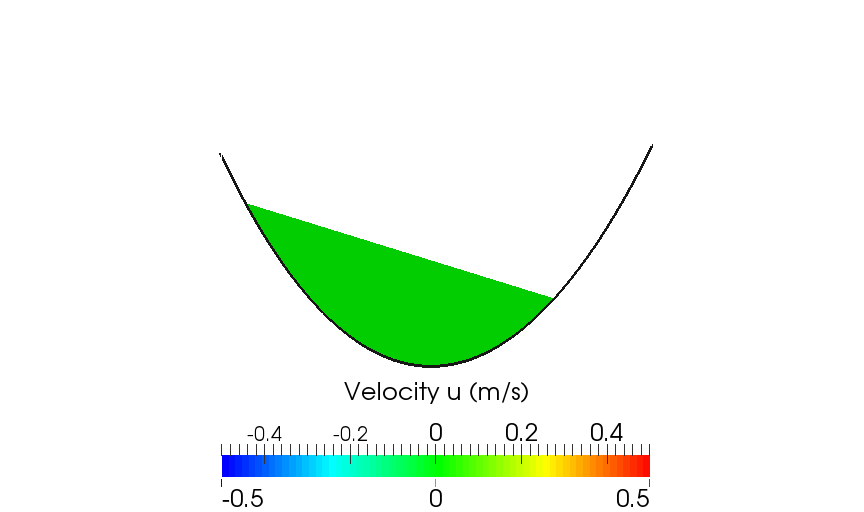
Figure 2: Initial conditions for the simulation of the “parabolic bowl” (parabolic bottom, water depth and null horizontal velocity).

To illustrate the behavior of the solution in such a situation, we give over Fig 3 the variations along time of the water depth at $x_{0}=0.8$ m for a mesh of 80 cells which is a rather coarse mesh.

In order to evaluate the convergence rate of the simulated solution towards the analytical one, we plot the error rate versus the space discretization. We have plotted in Fig. 4 the $\mbox{log}(L^{1}-error)$ over the water depth at time $T=10$ seconds – corresponding to more than 5 periods – versus $\mbox{log}(h_{0}/h_{i})$ for the first and second-order schemes and they are compared to the theoretical order. We denote by $h_{i}$ the average cell length, $h_{0}$ is the average cell length of the coarser space discretization. These errors have been computed on 6 meshes with $20$, $40$, $80$, $120$, $300$ and $400$ cells.

For this test case, the errors due to the time and space schemes are combined so the convergence rate of the simulated solution towards the analytical one is more difficult to analyze. Despite this fact, it appears that the computed convergence rates are close to the theoretical ones. It emphasizes the performance of the proposed numerical technique.

Over Fig 5, we have plotted the variations along time of the $\mbox{log}(L^{1}-error)$ over the water depth for the mesh with 80 cells calculated at node $x_{0}=0.8$ m i.e. the quantity

$$t\mapsto\log\left(100\frac{\left|H_{sim}(x_{0},t)-H_{anal}(x_{0},t)\right|}{H_{sim}(x_{0},t)}\right).$$

It appears that this quantity does not increase with time and remains bounded.

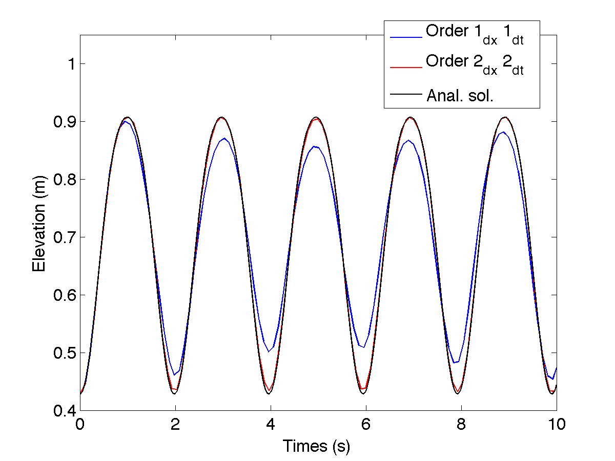
Figure 3: Parabolic bowl: variations of $t\mapsto H(0.8,t)$ - analytical solution and simulated one with the first order (space and time) and second order (space and time) schemes.

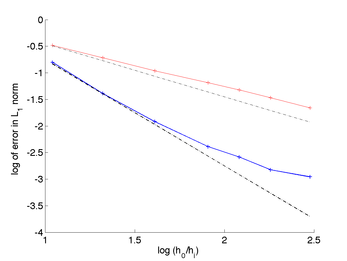
Figure 4: Parabolic bowl: convergence rates to the reference solution, 1^st order schemes (space and time) and 2^nd order schemes (space and time), ’-.’ theoretical order.

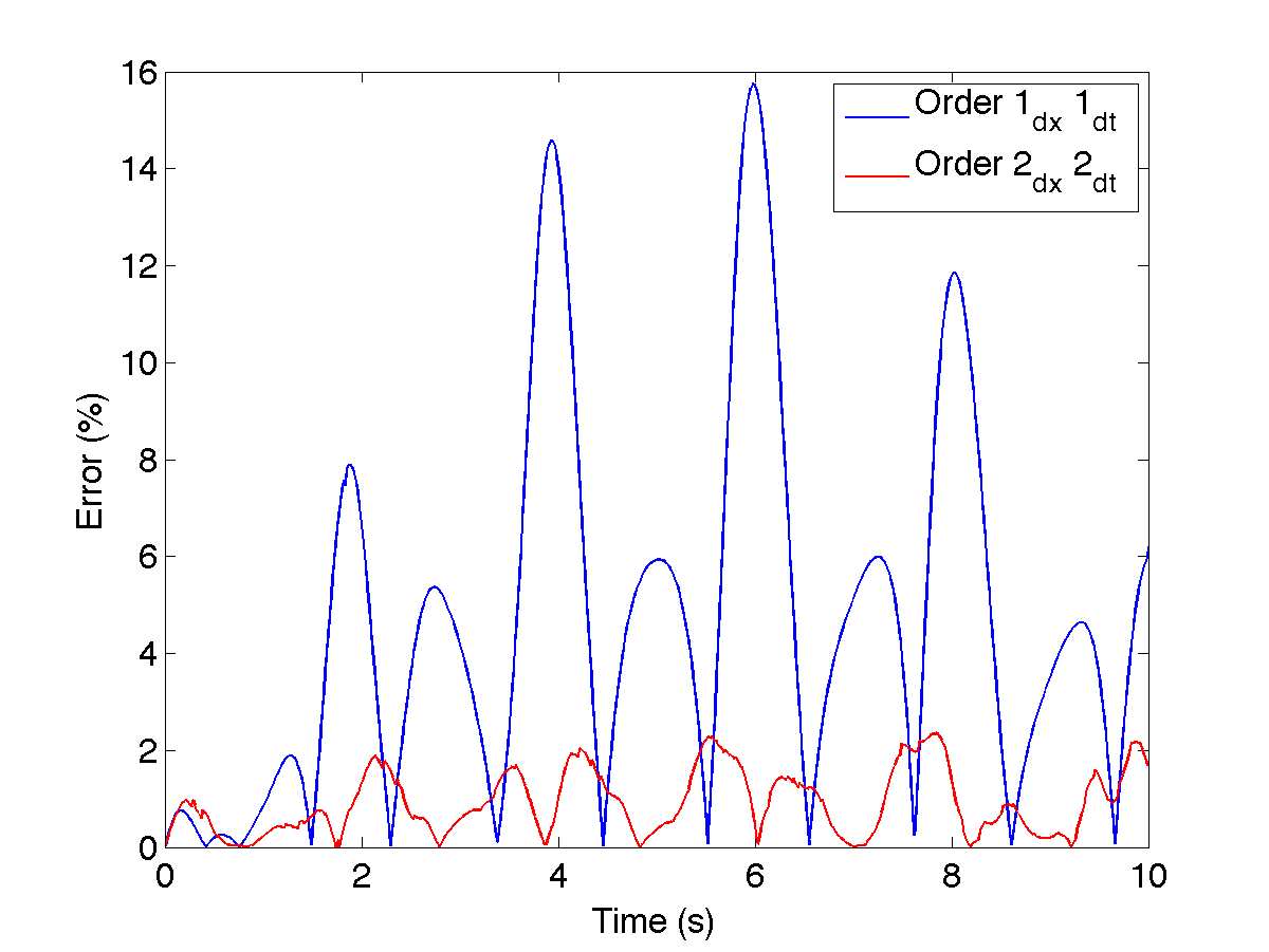
Figure 5: Parabolic bowl: variations along time of the error at node $x_{0}=0.8$ m, 1^st order schemes (space and time) and 2^nd order schemes (space and time).

7.2 The solitary wave

As in the previous paragraph, we are able to examine the convergence rate of the simulated solution towards the analytical one (given in paragraph 6.1.2).

We consider the analytical solution corresponding to the choices $H_{0}=1$ m, $l=1.7$ m, $d=1$ m. These choices lead to $a=0.5291$ m and $c_{0}=3.873$ m.s^-1. We compare the analytical solution and its simulated version at time $t=6$ s.

We have plotted in Fig. 6 the $\mbox{log}(L^{1}-error)$ over the water depth at time $T=6$ seconds versus $\mbox{log}(h_{0}/h_{i})$ for the first and second-order scheme and they are compared to the theoretical order. These errors have been computed on 7 meshes with $80$, $120$, $200$, $400$, $800$, $1600$ and $3200$ cells.

For the curves obtained over Fig. 6, the soliton is – at the initial instant – in the fluid domain meaning the numerical treatment of the boundary condition does not play a crucial role. Figure 7 is similar to Fig. 6 except that the soliton is not within the fluid domain at the initial instant but enters the channel by the left boundary. The convergence order of the scheme is examined at time $T=10$ seconds and the soliton arrives within the fluid domain after 4 seconds of simulation. Hence the soliton propagates during 6 seconds within the domain corresponding to the same situation as Fig. 6. Following 4.3.3, we have imposed a given flux at the entry of the domain. We notice that the convergence orders obtained over Figs. 6 and 7 are similar.

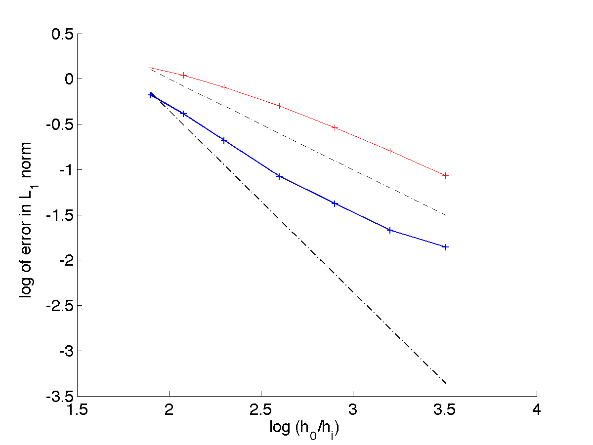
Figure 6: Soliton (interior of the domain): convergence rates to the reference solution, 1^st order schemes (space and time) and 2^nd order schemes (space and time), ’-.’ theoretical order.

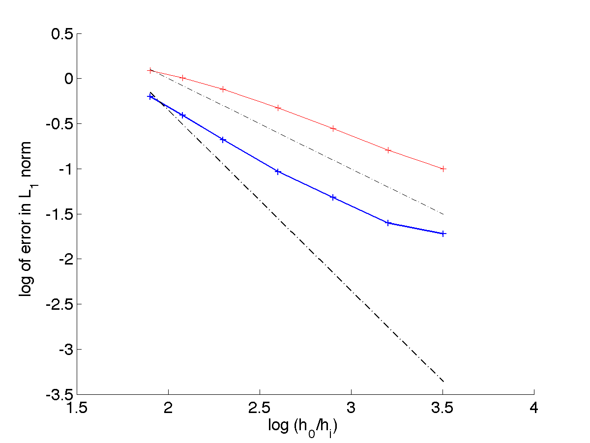
Figure 7: Soliton (entering in the domain): convergence rates to the reference solution, 1^st order schemes (space and time) and 2^nd order schemes (space and time), ’-.’ theoretical order.

8 Conclusion

In this paper we have proposed a robust and efficient numerical scheme for a non-hydrostatic shallow water type model approximating the incompressible Euler system with free surface.

The correction step is the key point of the scheme and especially the discretization of the shallow water type version of the gradient and divergence operators. A finite difference strategy has been used to discretize this correction step. In order to be able to treat 2d flows on unstructured meshes, a variational approximation of the correction step is required, it is presented and its numerical performance is evaluated in [1].

References

- [1] N. Aïssiouene, M.-O. Bristeau, E. Godlewski, and J. Sainte-Marie, A combined finite volume - finite element scheme for a dispersive shallow water system - https://hal.inria.fr/hal-01160718, June 2015.
- [2] B. Alvarez-Samaniego and D. Lannes, Large time existence for 3D water-waves and asymptotics, Invent. Math. 171 (2008), no. 3, 485–541. MR 2372806 (2009b:35324)
- [3] , A Nash-Moser theorem for singular evolution equations. Application to the Serre and Green-Naghdi equations, Indiana Univ. Math. J. 57 (2008), no. 1, 97–131. MR 2400253 (2010a:35016)
- [4] E. Audusse, F. Bouchut, M.-O. Bristeau, R. Klein, and B. Perthame, A fast and stable well-balanced scheme with hydrostatic reconstruction for Shallow Water flows, SIAM J. Sci. Comput. 25 (2004), no. 6, 2050–2065.
- [5] E. Audusse, F. Bouchut, M.-O. Bristeau, and J. Sainte-Marie, Kinetic entropy inequality and hydrostatic reconstruction scheme for the Saint-Venant system., (Accepted for publication in Math. Comp.) http://hal.inria.fr/hal-01063577/PDF/kin_hydrost.pdf, May 2015.
- [6] E. Audusse and M.-O. Bristeau, Transport of pollutant in shallow water flows : A two time steps kinetic method, ESAIM: M2AN 37 (2003), no. 2, 389–416.
- [7] , A well-balanced positivity preserving second-order scheme for Shallow Water flows on unstructured meshes, J. Comput. Phys. 206 (2005), no. 1, 311–333.
- [8] A.-J.-C. Barré de Saint-Venant, Théorie du mouvement non permanent des eaux avec applications aux crues des rivières et à l’introduction des marées dans leur lit, C. R. Acad. Sci. Paris 73 (1871), 147–154.
- [9] J.-L. Bona, T.-B. Benjamin, and J.-J. Mahony, Model equations for long waves in nonlinear dispersive systems, Philos. Trans. Royal Soc. London Series A 272 (1972), 47–78.
- [10] P. Bonneton, E. Barthelemy, F. Chazel, R. Cienfuegos, D. Lannes, F. Marche, and M. Tissier, Recent advances in Serre-Green Naghdi modelling for wave transformation, breaking and runup processes, European Journal of Mechanics - B/Fluids 30 (2011), no. 6, 589 – 597, Special Issue: Nearshore Hydrodynamics.
- [11] F. Bouchut, An introduction to finite volume methods for hyperbolic conservation laws, ESAIM Proc. 15 (2004), 107–127.
- [12] , Nonlinear stability of finite volume methods for hyperbolic conservation laws and well-balanced schemes for sources, Birkhäuser, 2004.
- [13] F. Bouchut, A. Mangeney-Castelnau, B. Perthame, and J.-P. Vilotte, A new model of Saint-Venant and Savage-Hutter type for gravity driven shallow water flows, C. R. Math. Acad. Sci. Paris 336 (2003), no. 6, 531 – 536.
- [14] F. Bouchut and M. Westdickenberg, Gravity driven shallow water models for arbitrary topography, Comm. in Math. Sci. 2 (2004), 359–389.
- [15] F. Brezzi, On the existence, uniqueness and approximation of saddle-point problems arising from Lagrangian multipliers, Rev. Française Automat. Informat. Recherche Opérationnelle Sér. Rouge 8 (1974), no. R-2, 129–151. MR 0365287 (51 #1540)
- [16] M.-O. Bristeau, N. Goutal, and J. Sainte-Marie, Numerical simulations of a non-hydrostatic Shallow Water model, Computers & Fluids 47 (2011), no. 1, 51–64.
- [17] M. O. Bristeau, A. Mangeney, J. Sainte-Marie, and N. Seguin, An energy-consistent depth-averaged Euler system: derivation and properties, Discrete Contin. Dyn. Syst. Ser. B 20 (2015), no. 4, 961–988.
- [18] M.-O. Bristeau and J. Sainte-Marie, Derivation of a non-hydrostatic shallow water model; Comparison with Saint-Venant and Boussinesq systems, Discrete Contin. Dyn. Syst. Ser. B 10 (2008), no. 4, 733–759.
- [19] M.O. Bristeau and B. Coussin, Boundary Conditions for the Shallow Water Equations solved by Kinetic Schemes, Research Report RR-4282, INRIA, 2001.
- [20] R. Camassa, D.D. Holm, and J.M. Hyman, A new integrable shallow water equation, Adv. Appl. Math. 31 (1993), 23–40.
- [21] F. Chazel, D. Lannes, and F. Marche, Numerical simulation of strongly nonlinear and dispersive waves using a Green–Naghdi model, J. Sci. Comput. 48 (2011), no. 1-3, 105–116.
- [22] A. J. Chorin, Numerical solution of the Navier-Stokes equations, Math. Comp. 22 (1968), 745–762. MR 0242392 (39 #3723)
- [23] A. Duran and F. Marche, Discontinuous-Galerkin discretization of a new class of Green-Naghdi equations, Communications in Computational Physics (2014), 130.
- [24] D. Dutykh, Th. Katsaounis, and D. Mitsotakis, Finite volume methods for unidirectional dispersive wave models, Internat. J. Numer. Methods Fluids 71 (2013), no. 6, 717–736. MR 3018287
- [25] S. Ferrari and F. Saleri, A new two-dimensional Shallow Water model including pressure effects and slow varying bottom topography, M2AN Math. Model. Numer. Anal. 38 (2004), no. 2, 211–234.
- [26] J.-F. Gerbeau and B. Perthame, Derivation of Viscous Saint-Venant System for Laminar Shallow Water; Numerical Validation, Discrete Contin. Dyn. Syst. Ser. B 1 (2001), no. 1, 89–102.
- [27] A. E. Green, N. Laws, and P. M. Naghdi, On the theory of water waves, Proc. Roy. Soc. (London) Ser. A 338 (1974), 43–55. MR 0349127 (50 #1621)
- [28] A.E. Green and P.M. Naghdi, A derivation of equations for wave propagation in water of variable depth, J. Fluid Mech. 78 (1976), 237–246.
- [29] D. Lannes and P. Bonneton, Derivation of asymptotic two-dimensional time-dependent equations for surface water wave propagation, Physics of Fluids 21 (2009), no. 1, 016601.
- [30] D. Lannes and F. Marche, A new class of fully nonlinear and weakly dispersive Green-Naghdi models for efficient 2D simulations, J. Comput. Phys. 282 (2015), 238–268. MR 3291451
- [31] O. Le Métayer, S. Gavrilyuk, and S. Hank, A numerical scheme for the Green-Naghdi model, J. Comp. Phys. 229 (2010), no. 6, 2034–2045.
- [32] A. Lucas, A. Mangeney, and J. P. Ampuero, Frictional weakening in landslides on earth and on other planetary bodies, Nature Communication 5 (2014), no. 3417.
- [33] N. Makarenko, A second long-wave approximation in the Cauchy-Poisson problem (in Russian), Dyn. Contin. Media 77 (1986), 56–72.
- [34] A. Mangeney, F. Bouchut, N. Thomas, J. P. Vilotte, and M.-O. Bristeau, Numerical modeling of self-channeling granular flows and of their levee-channel deposits, Journal of Geophysical Research - Earth Surface 112 (2007), no. F02017. MR 1975092 (2004c:76017)
- [35] A. Mangeney-Castelnau, F. Bouchut, J. P. Vilotte, E. Lajeunesse, A. Aubertin, and M. Pirulli, On the use of Saint-Venant equations to simulate the spreading of a granular mass, Journal of Geophysical Research: Solid Earth 110 (2005), no. B09103.
- [36] F. Marche, Derivation of a new two-dimensional viscous shallow water model with varying topography, bottom friction and capillary effects, European Journal of Mechanic /B 26 (2007), 49–63.
- [37] J. Miles and R. Salmon, Weakly dispersive nonlinear gravity waves, J. Fluid Mech. 157 (1985), 519–531. MR 808127 (86m:76021)
- [38] O. Nwogu, Alternative form of Boussinesq equations for nearshore wave propagation, Journal of Waterway, Port, Coastal and Ocean Engineering, ASCE 119 (1993), no. 6, 618–638.
- [39] D.H. Peregrine, Long waves on a beach, J. Fluid Mech. 27 (1967), 815–827.
- [40] B. Perthame, Kinetic formulation of conservation laws, Oxford University Press, 2002.
- [41] B. Perthame and C. Simeoni, A kinetic scheme for the Saint-Venant system with a source term, Calcolo 38 (2001), no. 4, 201–231.
- [42] J. Sainte-Marie, Vertically averaged models for the free surface Euler system. Derivation and kinetic interpretation, Math. Models Methods Appl. Sci. (M3AS) 21 (2011), no. 3, 459–490.
- [43] C. H. Su and C. S. Gardner, Korteweg-de Vries equation and generalizations. III. Derivation of the Korteweg-de Vries equation and Burgers equation, J. Mathematical Phys. 10 (1969), 536–539. MR 0271526 (42 #6409)