Cavity-induced modifications of molecular structure in the strong coupling regime

Abstract

In most theoretical descriptions of collective strong coupling of organic molecules to a cavity mode, the molecules are modeled as simple two-level systems. This picture fails to describe the rich structure provided by their internal rovibrational (nuclear) degrees of freedom. We investigate a first-principles model that fully takes into account both electronic and nuclear degrees of freedom, allowing an exploration of the phenomenon of strong coupling from an entirely new perspective. First, we demonstrate the limitations of applicability of the Born-Oppenheimer approximation in strongly coupled molecule-cavity structures. For the case of two molecules, we also show how dark states, which within the two-level picture are effectively decoupled from the cavity, are indeed affected by the formation of collective strong coupling. Finally, we discuss ground-state modifications in the ultra-strong coupling regime and show that some molecular observables are affected by the collective coupling strength, while others only depend on the single-molecule coupling constant.

I Introduction

Strong coupling in quantum electrodynamics is a well-known phenomenon that occurs when the coherent energy exchange between a light mode and quantum emitters is faster than the decay and decoherence of either constituent Thompson et al. (1992); Weisbuch et al. (1992). The excitations of the system are then hybrid light-matter excitations, so-called polaritons, that combine the properties of both constituents. Exploiting these properties enables new applications such as polariton condensation under collective strong coupling to excitons (excited electron-hole pairs) in semiconductors Kasprzak et al. (2006); Balili et al. (2007) and organic materials Kéna-Cohen and Forrest (2010); Plumhof et al. (2014); Daskalakis et al. (2014). Organic materials present a particularly favorable case, as the Frenkel excitons in these materials possess large binding energies, large dipole moments, and can reach high densities. This enables Rabi splittings $\Omega_{R}$ (the energy splitting between the polaritons) up to more than $1$ eV Lidzey et al. (1998); Schwartz et al. (2011); Kéna-Cohen et al. (2013), a significant fraction of the uncoupled transition energy. These properties allow for strong coupling to many kinds of electromagnetic (EM) modes Törmä and Barnes (2015), such as cavity photons Lidzey et al. (1998); Schwartz et al. (2011); Kéna-Cohen et al. (2008), surface plasmon polaritons Bellessa et al. (2004); Dintinger et al. (2005); Hakala et al. (2009); Vasa et al. (2010), surface lattice resonances Rodriguez et al. (2013); Väkeväinen et al. (2014), or localized surface plasmons Baudrion et al. (2013); Zengin et al. (2015).

Figure 1: Illustration of energy level structure of a bare complex molecule and the hybrid states that result in the strong coupling regime with a photonic mode of energy $\hbar\omega_{c}$, resonant with the molecular excitation.

While organic molecules are thus uniquely suited to achieving strong coupling, they are not simple two-level quantum emitters, but rather have a complicated level structure including not only electronic excitations, but also rovibrational degrees of freedom (schematically depicted in Fig. 1). It has been experimentally demonstrated that strong coupling can modify this structure, in the sense that material properties and chemical reaction rates change Hutchison et al. (2012, 2013); Wang et al. (2014). However, the models used to describe strong coupling are often focused on macroscopic descriptions Carusotto and Ciuti (2013), and most microscopic models do treat organic molecules as two-level systems (see Michetti et al. (2015) for a recent review). When the rovibrational degrees of freedom are taken into account, this is often done using effective decay and dephasing rates González-Tudela et al. (2013), with a few works explicitly including a phononic degree of freedom Mazza et al. (2013); Ćwik et al. (2014). All of these approaches only provide limited insight into the effects of strong coupling on molecular structure.

In the present work, we thus aim for a microscopic description of strong coupling with organic molecules. We introduce a simple first-principles model that fully describes nuclear, electronic and photonic degrees of freedom, but can be solved without approximations. This allows us to provide a simple picture for understanding the induced modification of molecular structure.

In section II, after introducing the model, we discuss under which conditions and in which form the Born-Oppenheimer approximation (BOA) Born and Oppenheimer (1927); Tully (2000) is valid in the strong coupling regime for a single molecule. The BOA is widely used in molecular and solid state physics and quantum chemistry, and provides a simple picture of nuclei moving on effective potential energy surfaces (PES) generated by the electrons, which underlies most of the current understanding of chemical reactions Tully (2000). However, the BOA depends on the separation of electronic and nuclear energy scales, i.e., the fact that electrons typically move much faster than nuclei. It could thus conceivably break down when an additional, intermediate timescale is introduced under strong coupling to an EM mode. The speed of energy exchange between field and molecules is determined by the Rabi frequency $\Omega_{R}$, and typical experimental values of hundreds of meV land squarely between typical nuclear ($\simeq 100~{}$meV) and electronic ($\simeq 2$ eV) energies. We show that the BOA indeed breaks down at intermediate Rabi splittings, but remains valid when $\Omega_{R}$ becomes large enough. For cases where it breaks down, we show that the non-BO coupling terms can be obtained to a good approximation without requiring knowledge of the electronic wave functions.

In section III, we focus on the effects of strong coupling when more than one molecule is involved, using two molecules as the simplest test case. In experiments, strong coupling is achieved by collective coupling to a large number of molecules, under which the Rabi frequency is enhanced by a factor of $\sqrt{N}$. The number of emitters $N$ is on the order of $\gtrsim 10^{5}$ within cavities Lidzey et al. (1998); Schwartz et al. (2011); Kéna-Cohen et al. (2008, 2013), with plasmonic nanoparticle modes allowing to reduce this to $N\sim 100$ Zengin et al. (2015). In this context, it is well known that only a small fraction of the collective electronic excitations are strongly coupled Houdré et al. (1996); Agranovich et al. (2011); Michetti et al. (2015), with a large number of “dark” or “uncoupled” modes that show no mixing with the EM mode and no energy shift. We show that even these dark modes are affected by strong coupling, with the nuclear motion of separated molecules becoming correlated.

In section IV, we focus on the so-called ultrastrong coupling regime, where the Rabi frequency reaches a significant fraction of the electronic transition energy, as achieved in experiments. In this regime, not just excited-state, but also ground-state properties are modified—for example, the ground state acquires a photonic contribution De Liberato et al. (2007); Carusotto and Ciuti (2013). Accordingly, we discuss whether ground-state chemical properties of organic molecules could be modified by strong coupling. This also allows us to partially answer the open question what strong coupling means for modifications of chemical structure George et al. (2015), i.e., whether “all” molecules are modified by it, or only a small subset, or whether we necessarily have to invoke collective modes even when discussing “single-molecule” effects. We show that while some observables, such as energy shifts, are determined by the collective Rabi frequency, but other observables, such as the shift in ground-state bond length, are instead determined by the single-molecule coupling strength $\propto\Omega_{R}/\sqrt{N}$.

For simplicity, we only treat a single EM mode and completely neglect dissipation in the following. We use atomic units unless stated otherwise ($4\pi\varepsilon_{0}=\hbar=m_{e}=e=1$, with electron mass $m_{e}$ and elementary charge $e$).

II Single Molecule

In this section, we introduce our model for a single molecule coupled to an EM mode. Due to the exponential scaling with the degrees of freedom, solving the full time-independent Schrödinger equation for an organic molecule without the BOA is an extremely challenging task that even modern supercomputers can only handle for very small molecules. We thus employ a reduced-dimensionality model that we can easily solve, both for the bare molecule and after coupling to an EM mode.

II.1 Method

II.1.1 Bare molecule

We work within the single-active-electron approximation (SAE), in which all but one electron are frozen around the nuclei, and additionally restrict the motion of the active electron to one dimension, $x$. Furthermore, we only treat one nuclear degree of freedom, the reaction coordinate $R$. This could correspond to the movement of a single bond in a molecule, but can equally well represent collective motion, e.g., the breathing mode of a carbon ring. The effective molecular Hamiltonian then highly resembles that of a one-dimensional diatomic molecule,

$$\hat{H}_{m}=\hat{T}_{n}+\hat{T}_{e}+V_{en}(x;R)+V_{nn}(R),$$ (1)

where $\hat{T}_{n}=\frac{\hat{P}^{2}}{2M}$ and $\hat{T}_{e}=\frac{\hat{p}^{2}}{2}$ are the nuclear and electronic kinetic energy operators (with $\hat{P}$, $\hat{p}$ the corresponding momenta), and $M$ is the nuclear mass. The potentials $V_{en}(x,R)$ and $V_{nn}(R)$ represent the effective electron-nuclei and internuclear interactions, where we assume two nuclei located at $x=\pm R/2$. These potentials encode the information about the frozen electrons as well as the nuclear structure of the molecule, and can be adjusted to approximately represent different molecules.

The electron-nucleus interaction $V_{en}$ contains the interaction of the active electron with each nucleus, as well as with the frozen electrons surrounding it. Assuming a nuclear charge of $Z$, we have $2Z-1$ frozen electrons distributed across the two nuclei. For large distances, the active electron should thus feel a Coulomb potential with an effective charge of $\frac{1}{2}$ from each nucleus. Conversely, at very small distances, the active electron is not affected by the cloud of frozen electrons and feels an effective charge of $Z$. Since we are working within one dimension, we use a soft Coulomb potential to take into account that the electron avoids the singularity at the nucleus. We choose a simple model potential fulfilling these conditions:

$$V_{en}(r)=-\frac{\frac{1}{2}+(Z-\frac{1}{2})e^{-\frac{r}{r_{0}}}}{\sqrt{r^{2}+\alpha^{2}}},$$ (2)

where $\alpha$ is the softening parameter, $r_{0}$ describes the localization of the frozen electrons around the nucleus, and $r$ is the electron-nucleus distance. The total potential is thus $V_{en}(x,R)=V_{en}(|x-R/2|)+V_{en}(|x+R/2|)$.

The internuclear potential $V_{nn}(R)$ represents the interaction between the nuclei and the $2Z-1$ frozen electrons, i.e., the ground state potential energy surface of the molecular ion. We model this surface by a Morse potential

$$V_{nn}(R)=D_{e}\left(1-e^{A(R-R_{0})}\right)^{2},$$ (3)

which adds three new parameters: the dissociation energy $D_{e}$, the equilibrium distance $R_{0}$ and the width of the potential well $A$. By tuning the seven free parameters we have at our disposal ($M$, $Z$, $\alpha$, $r_{0}$, $D_{e}$, $R_{0}$ and $A$), we can approximately fit both the electronic and vibrational structure and absorption spectrum to those of real organic molecules.

We can now solve the stationary Schrödinger equation $\hat{H}_{m}\Psi(x,R)=E\Psi(x,R)$ for the bare-molecule Hamiltonian Eq. (missing) 1 without further approximations by representing $\hat{H}_{m}$ on a two-dimensional grid in $x$ and $R$. For a bare molecule, the results are virtually identical to those obtained within the BOA and thus not shown here.

We next give a short description of the Born-Oppenheimer approximation for completeness (see Born and Oppenheimer (1927); Tully (2000) for more details). As mentioned above, the basic idea is to exploit the separation between nuclear and electronic timescales and to assume that the electrons perfectly follow nuclear rearrangements without changing state (i.e., adiabatically). This is achieved by separating the Hamiltonian into the nuclear kinetic energy $\hat{T}_{n}$ and an electronic Hamiltonian $\hat{H}_{e}(x;R)=\hat{H}_{m}(x,R)-\hat{T}_{n}$ that only depends on $R$ parametrically. Diagonalizing $\hat{H}_{e}$ yields a set $\{\phi_{k}\}$ of electronic eigenstates for every $R$, with $\hat{H}_{e}(x;R)\phi_{k}(x;R)=E_{k}(R)\phi_{k}(x;R)$. Without loss of generality, each total eigenstate $\Psi^{i}$ can be represented by $\Psi^{i}(x,R)=\sum_{k}\phi_{k}(x;R)\chi^{i}_{k}(R)$. Inserting this expansion into the Hamiltonian Eq. (missing) 1 leads to a set of coupled differential equations,

$$(\hat{T}_{n}+E_{k})\chi^{i}_{k}(R)+\sum_{k^{\prime}}\hat{C}_{n}^{kk^{\prime}}\chi^{i}_{k^{\prime}}=E\chi^{i}_{k}(R),$$ (4)

with nuclear motion taking place on potential energy surfaces (PES) $E_{k}(R)$ that are coupled through correction terms $\hat{C}_{n}^{kk^{\prime}}=\langle\phi_{k}|\hat{T}_{n}|\phi_{k^{\prime}}\rangle_{x}+\langle\phi_{k}|\frac{\hat{P}}{2M}|\phi_{k^{\prime}}\rangle_{x}\hat{P}$, where the subscript $x$ indicates that the integration in the brakets is only over the electronic coordinate. The Born-Oppenheimer approximation now consists in neglecting the intersurface couplings $\hat{C}_{n}^{kk^{\prime}}$, which can be shown to be small when the electronic levels are well-separated. This gives a set of independent PES $E_{k}(R)$ on which the nuclei move, where each eigenstate is a product of a single electronic and nuclear wave function, $\Psi^{i}_{k}(x,R)=\phi_{k}(x;R)\chi^{i}_{k}(R)$. The different nuclear functions on each electronic curve correspond to rotational or vibrational excitation. This picture of nuclear motion on PES is extremely powerful and underlies most of the current understanding of chemical reactions Tully (2000). The question of its validity in the strong coupling regime is thus of central importance for the possible modification of chemical reactions and structure through strong coupling.

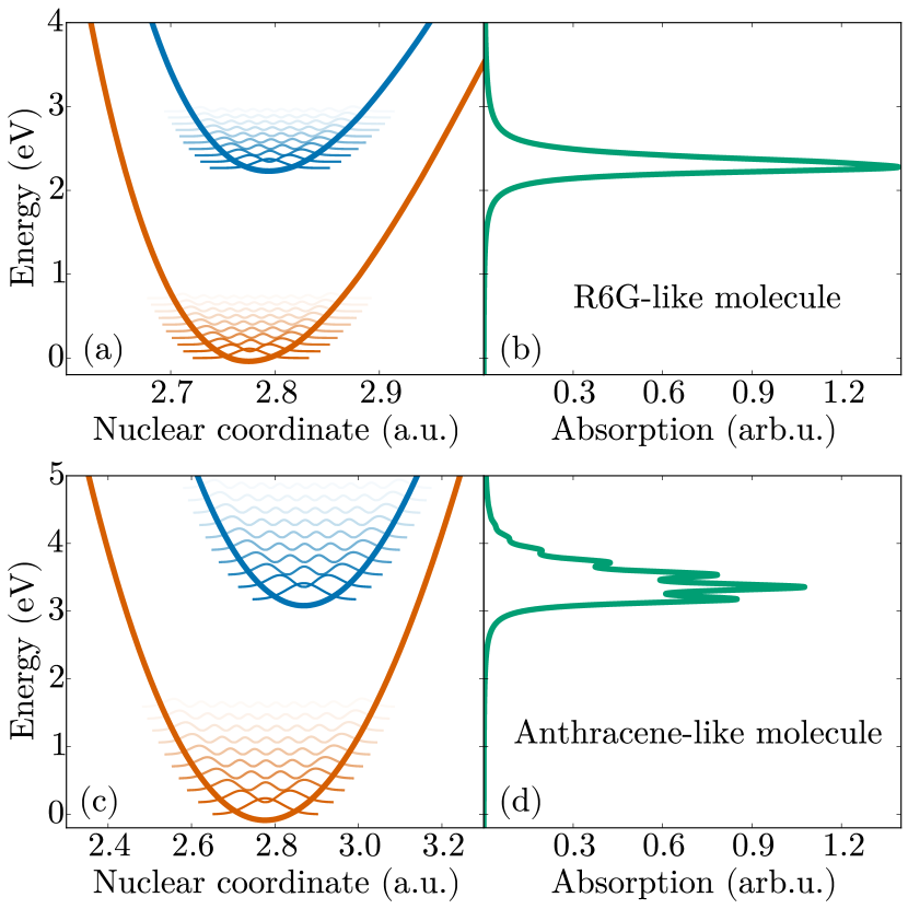
Figure 2: Bare-molecule potential energy surfaces of the two first electronic states in the BOA for (a) the rhodamine 6G-like model molecule and (c) the anthracene-like model molecule. The vibrational levels and associated nuclear probability densities are represented on top of the PES. (b) and (d): Absorption spectrum for the (b) R6G-like and (d) anthracene-like molecule in arbitrary units.

In the following, we will focus on two model molecules, which approximately reproduce the absorption spectra of rhodamine 6G (R6G) and anthracene molecules that are commonly used in experimental realizations of strong coupling Kéna-Cohen et al. (2008); Hakala et al. (2009); Rodriguez et al. (2013). Only the first two PES, corresponding to the ground $E_{g}(R)$ and first electronically excited $E_{e}(R)$ state, play a role in the results discussed in the following. They are shown in Fig. 2a and Fig. 2c, together with the nuclear probability densities $|\chi(R)|^{2}$ for the lowest vibrational levels on each PES. Importantly, the two models differ significantly in two relevant quantities: the vibrational mode frequency $\omega_{vib}$ and the offset $\Delta R$, i.e., the change in equilibrium distance between the ground and excited PES. This offset is related to the strength of the electron-phonon interaction and influences the Stokes shift between emission and absorption May and Kühn (2011). The R6G-like model has relatively small vibrational spacing $\omega_{vib}\approx 70$ meV and small offset $\Delta R\approx 0.018$ a.u., while the anthracene-like model has large vibrational spacing $\omega_{vib}\approx 180$ meV and large offset $\Delta R\approx 0.092$ a.u.. Accordingly, their absorption spectra (Fig. 2b and Fig. 2d, obtained from Eq. (missing) 6 below) are qualitatively different, with anthracene showing a broader absorption peak with well-resolved vibronic subpeaks.

II.1.2 Molecule-photon coupling

We now add a photonic mode and its coupling to the molecule (within the dipole approximation) into the molecular Hamiltonian,

$$\hat{H}_{mc}=\hat{H}_{m}+\omega_{c}\hat{a}^{\dagger}\hat{a}+g\hat{\mu}(\hat{a}^{\dagger}+\hat{a}),$$ (5)

where $\hat{\mu}$ is the dipole operator of the molecule ($\hat{\mu}=x$ in our case), $\hat{a}^{\dagger}$ and $\hat{a}$ are the creation and annihilation operators for the bosonic EM field mode, $\omega_{c}$ is its frequency, and $g$ is the coupling strength constant, given by the electric field amplitude (along the $x$-axis) of a single photon. In the following, we always set the photon energy $\omega_{c}$ to achieve “zero detuning”, with $\omega_{c}$ at the absorption maximum of the molecule. This gives $\omega_{c}\approx E_{e}(R_{e})-E_{g}(R_{e})$, where $R_{e}$ is the equilibrium position at which $E_{g}(R)$ has its minimum.

To provide some context for the field strengths used in the following, we note that for a typical microcavity with a mode volume $V\approx\lambda_{c}^{3}$, one obtains $g=\sqrt{\frac{\hbar\omega_{c}}{2\varepsilon_{0}V}}\approx 1.34\times 10^{-7}\omega_{c}^{2}$ a.u. (for $\omega_{c}$ given in eV). However, for an effective mode volume close to the current record achieved in plasmonic nano-antennas, $V\approx 1.3\times 10^{-7}\lambda_{c}^{3}$ Kim et al. (2015), the single-particle coupling reaches $g\approx 3.72\times 10^{-4}\omega_{c}^{2}$ a.u. ($\omega_{c}$ again in eV). We furthermore note that the ground-to-excited state dipole transition moments of our model molecules are on the order of $1~{}\mathrm{a.u.}\approx 2.54$ D, i.e., almost an order of magnitude smaller than in typical organic molecules Moll et al. (1995).

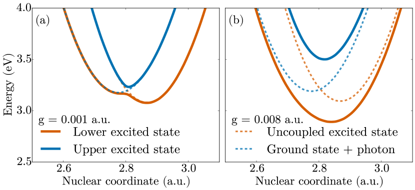
Figure 3: Strongly coupled electronic PES (solid lines) in the singly excited subspace, for the anthracene-like molecule for (a) $g=0.001$ a.u. and (b) $g=0.008$ a.u.. The dashed lines show the corresponding uncoupled states: A molecule in the first excited state, $E_{e}(R)$, and a molecule in the ground state with one photon present, $E_{g}(R)+\omega_{c}$.

Compared to the bare-molecule case, the Hamiltonian now includes a new degree of freedom, the photon number $n\in\{0,1,2,\ldots\}$, with the system eigenstates defined by $\hat{H}_{mc}\Psi(x,n,R)=E\Psi(x,n,R)$. As discussed above, the typical energies associated with strong coupling in organic molecules are somewhere between the nuclear and electronic energies. A priori, this suggests two options of performing the BOA: the additional terms introduced by the photonic degree of freedom could be grouped either with the “slow” nuclear motion or with the “fast” electronic Hamiltonian. However, as the photon couples to the electron, grouping it with the nuclear terms necessarily leads to additional off-diagonal terms in Eq. (missing) 4, and no independent PES on which the nuclei move could be obtained. Consequently, the only way to maintain the usefulness of the BOA is to include the photonic degree of freedom within the electronic Hamiltonian, leading to a new set of “strongly coupled PES”.

We first focus on the singly excited subspace, within which the splitting between polaritons is observed. Here, either the molecule is electronically excited and no photons are present, or the molecule is in its electronic ground state and the photon mode is singly occupied. At zero coupling ($g=0$), this gives two uncoupled PES ($E_{e}(R)$ and $E_{g}(R)+\omega_{c}$, dashed curves in Fig. 3) that cross close to $R_{e}$ for our choice of $\omega_{c}$. When the electron-photon coupling is non-zero but small, a narrow avoided crossing develops instead (solid lines in Fig. 3a), while for large coupling strengths, the energy exchange between photonic and electronic degrees of freedom is so fast that we observe two entirely new PES (Fig. 3b), which can not be easily associated with either of the uncoupled PES. Instead, they become hybrid polaritonic PES that contain a mixture of electronic and photonic excitation, the hallmark of the strong coupling regime.

As discussed above, the BOA is known to be valid when two PES are sufficiently separated from each other. This implies that the BOA breaks down when $g$ is small and the two PES possess a narrow avoided crossing. This in itself is not a surprising result—when the electron-photon coupling is very small, the system is not even in the strong coupling regime, and the photon mode is better treated as a small perturbation. Fortunately, the weak coupling regime is also not interesting from the standpoint of understanding or modifying molecular structure through strong coupling. The real question thus must be: How strong does the electron-photon coupling have to be for the BOA to be valid, and is this condition fulfilled for realistic experimental parameters? In order to better quantify the agreement between the BOA and the full solution, we next turn to an easily measured physical observable: the absorption spectrum.

II.2 Absorption

The absorption cross section at frequency $\omega$ can be calculated from the polarizability as Rescigno and McKoy (1975); Bonin and Kresin (1997)

$$\sigma(\omega)=\frac{4\pi\omega}{c}\operatorname{Im}\lim_{\varepsilon\to 0}\sum_{k}\frac{|\langle\psi_{k}|\hat{\mu}|\psi_{0}\rangle|^{2}}{\omega_{k}-\omega_{0}-\omega-i\varepsilon},$$ (6)

where the sum runs over all eigenstates $|\psi_{k}\rangle$ of the system (with energies $\omega_{k}$) and $|\psi_{0}\rangle$ is the ground state. As we do not include incoherent processes in our calculation, this would give $\delta$-like peaks in the absorption cross section. In the plots shown in the following, we instead introduce a phenomonological width representing losses and pure dephasing by setting $\varepsilon$ to a small non-zero value, such that the absorption cross section becomes a sum of Lorentzians. For the bare-molecule case without coupling to an EM mode, the absorption spectra of our two model molecules approximately agree with those of R6G (Fig. 2b, Rodriguez et al. (2013)) and anthracene (Fig. 2d, Kéna-Cohen et al. (2008)).

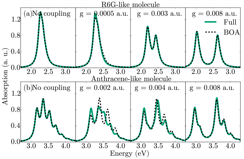
Figure 4: Absorption cross sections of a single molecule, calculated using the full Hamiltonian without approximation (solid green lines) and within the BOA (dashed black lines). Results are shown for the (a) R6G-like and (b) anthracene-like model molecules, for several values of the coupling strength $g$.

In Fig. 4, we compare the absorption cross sections under strong coupling as obtained from a full calculation without approximations to those obtained within the BOA, for a range of coupling strengths $g$ to the EM mode. Even for relatively small $g$, the BOA is found to agree almost perfectly with the full results for the R6G-like molecule with small vibrational spacing (Fig. 4a). However, for the anthracene-like molecule with a high-frequency vibrational mode and large offset $\Delta R$, the BOA only agrees with the full resul for relatively large values of $g$, where the Rabi splitting $\Omega_{R}$ (as defined by the energy difference between the two “polariton” peaks in the absorption spectrum) is appreciably larger than the vibrational frequency $\omega_{vib}\approx 180$ meV (Fig. 4b).

This qualitative observation can be quantified by comparing the correction terms $\hat{C}_{n}^{kk^{\prime}}$ in Eq. (missing) 4 with the energy difference between the anticrossing PES at the point of closest approach. In appendix A, we present a model that achieves this without any explicit knowledge of the electronic wave functions. It relies on the observation that close to the anticrossing, the coupled (polariton) states switch character between the two uncoupled states, while the “intrinsic” $R$-dependence of the uncoupled electronic states can be neglected. The correction terms $\hat{C}_{n}^{kk^{\prime}}$ can then be obtained just from the knowledge of $E_{g}(R)$, $E_{e}(R)$, and $\mu_{eg}(R)$, where $\mu_{eg}(R)$ is the electronic transition dipole between the ground and excited state. By approximating $E_{g}(R)$ and $E_{e}(R)$ as harmonic oscillators, the correction terms can be analytically evaluated and are found to be negligible under the condition that $\Delta R\omega_{vib}^{2}/\Omega_{R}^{2}$ is small compared to the nuclear momentum of the relevant eigenstates. This demonstrates that the model molecules present two opposite cases for the applicability of the BO approximation: our R6G-like molecule has a relatively small vibrational spacing $\omega_{vib}\approx 70$ meV and small electron-phonon coupling, $\Delta R\approx 0.018$ a.u., while our anthracene-like model molecule has a large vibrational spacing $\omega_{vib}\approx 180$ meV and large electron-phonon coupling, $\Delta R\approx 0.092$ a.u.. We note that in many experiments involving organic molecules, $\Omega_{R}\gtrsim 500$ meV Schwartz et al. (2011); Kéna-Cohen et al. (2013) is significantly larger than typical vibrational frequencies $\omega_{vib}\lesssim 200$ meV Shimanouchi (1972). This shows that the intuitive picture of nuclear dynamics unfolding on uncoupled Born-Oppenheimer potential energy surfaces can often be applied to understand the modification of molecular chemistry induced by strong coupling. Additionally, even when the BOA breaks down, the model presented in appendix A can be used to obtain the non-BO coupling terms without requiring knowledge of the electronic wave functions. The only necessary input are the uncoupled PES and the associated transition dipole moments. Even for relatively large molecules, these can be obtained using the standard methods of quantum chemistry or density functional theory.

III Two molecules

In the previous section, we showed that on the single-molecule level, the BOA is valid as long as the Rabi splitting $\Omega_{R}$ is large enough. However, current experiments are performed with large numbers of molecules, where coherent superpositions of electronic excitations (bright “Dicke states” Dicke (1954)) couple strongly to the photonic mode(s), while other superpositions give uncoupled or “dark” modes. It is thus important to consider if and how our conclusions have to be modified when more than a single molecule is involved in strong coupling.

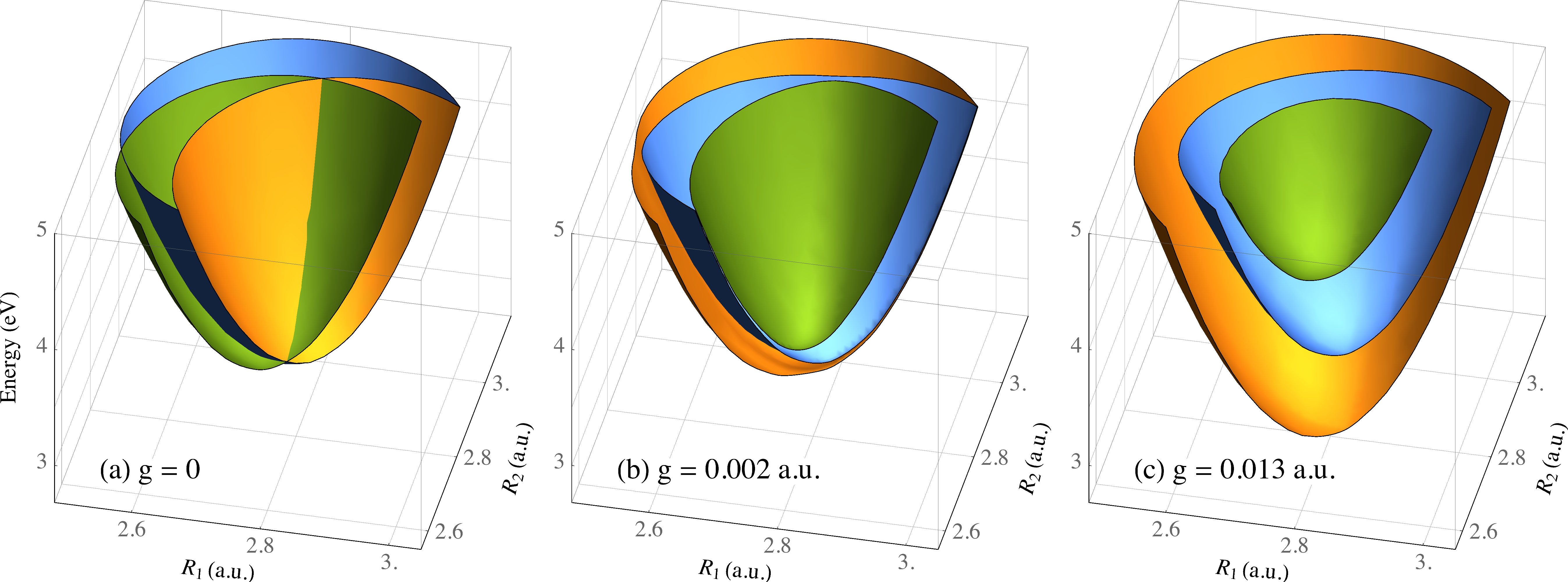
Figure 5: (a) Uncoupled potential energy surfaces of two anthracene-like molecules in the singly excited subspace: $E_{eg0}(R_{1},R_{2})$ (orange), $E_{eg0}(R_{1},R_{2})$ (blue), and $E_{gg1}(R_{1},R_{2})$ (green). (b) Coupled PES for $g=0.002$ a.u. and (c) $g=0.013$ a.u., corresponding to the lower polariton (orange), dark state (blue), and upper polariton (green). For clarity, only parts where $R_{1}<R_{2}$ are shown (note that the system is symmetric under the exchange $R_{1}\leftrightarrow R_{2}$).

For later reference, we give a quick overview of the theory when using an ensemble of two-level emitters coupled to a photonic mode, i.e., the many-particle Jaynes-Cummings (JC) model Jaynes and Cummings (1963), also known as the the Tavis-Cummings model Tavis and Cummings (1967). Its Hamiltonian within the rotating-wave approximation is

$$\hat{H}_{JC}=\omega_{c}\hat{a}^{\dagger}\hat{a}+\sum_{i}\omega_{i}\hat{c}^{\dagger}_{i}\hat{c}_{i}+\sum_{i}g_{i}(\hat{a}\hat{c}^{\dagger}_{i}+\hat{a}^{\dagger}\hat{c}_{i}),$$ (7)

where $\omega_{i}$ is the energy of emitter $i$ with destruction (creation) operator $\hat{c}_{i}$ ($\hat{c}_{i}^{\dagger}$), and the $g_{i}$ describe the emitter-photon couplings. For identical emitters ($\omega_{i}=\omega_{m}$, $g_{i}=g$), the resulting eigenstates in the single-excitation subspace are given by two polaritons $|\pm\rangle=\frac{1}{\sqrt{2}}(\hat{a}^{\dagger}|0\rangle\pm|B\rangle)$, symmetric and antisymmetric combinations of the photonic mode with the emitter bright state $|B\rangle=\frac{1}{\sqrt{N}}\sum_{i}\hat{c}_{i}^{\dagger}|0\rangle$. At zero detuning ($\omega_{c}=\omega_{m}$), the polariton energies are given by $\omega_{\pm}=\omega_{m}\pm\Omega_{R}/2$, where $\Omega_{R}=2g\sqrt{N}$ is the collective Rabi splitting. The $N-1$ superpositions of emitter states orthogonal to $|B\rangle$ are dark states that are not coupled to the photonic mode, with energies identical to the uncoupled emitters, $\omega_{DS}=\omega_{m}$. Note that in configurations with many photonic modes (e.g., planar cavities), more than one emitter state is coupled to the photonic mode (typically at low in-plane momentum), but there remain many uncoupled (dark) modes at higher in-plane momentum Michetti et al. (2015); Agranovich et al. (2011). There is an ongoing discussion in the literature on whether the “dark” modes are affected by strong coupling as well, or whether they should be thought of as completely unmodified emitter states. We will show below that when taking the internal structure of the emitters (molecules) into account, even the “dark” modes are affected by strong coupling and the nuclear dynamics of separate molecules become correlated.

We now treat the case of two model molecules, which can still be solved exactly within our approach, but which displays many of the effects of many-molecule strong coupling. As in the JC model, we assume that the two molecules both couple to the same photonic mode, but do not directly interact with each other, giving

$$\hat{H}_{mc}^{2m}=\omega_{c}\hat{a}^{\dagger}\hat{a}+\sum_{j=1,2}\left(\hat{H}_{m}^{(j)}+g\hat{\mu}^{(j)}(\hat{a}^{\dagger}+\hat{a})\right),$$ (8)

where the superscripts $j$ indicate the molecule on which the operator acts. Directly diagonalizing this Hamiltonian in the “raw” basis $\{x_{1},R_{1},x_{2},R_{2},n\}$ is already a formidable computational task for typical grid sizes. We thus calculate the full solution by first diagonalizing the single-molecule Hamiltonian, $\hat{H}_{m}=\sum_{k}E_{k}|k\rangle\langle k|$, and including only a relevant subset of eigenstates $\{k\}$ for each molecule in the total basis $\{k_{1},k_{2},n\}$. The number of necessary eigenstates to obtain completely converged results is quite small ($\approx 30$ per molecule). However, this approach only provides limited insight into the dynamics of the strongly coupled system, especially regarding nuclear motion.

We thus again apply the Born-Oppenheimer approximation by separating the nuclear kinetic energy terms and diagonalizing the remaining Hamiltonian parametrically as a function of $R_{1}$ and $R_{2}$. Similar to above, instead of working in the $\{x_{1},x_{2},n\}$ basis for each combination $(R_{1},R_{2})$, we prediagonalize the single-molecule electronic Hamiltonian $\hat{H}_{e}(x;R)=\sum_{k}E_{k}(R)|k(R)\rangle\langle k(R)|$, where (for the cases discussed here) the sum only has to include the ground and first excited states to achieve convergence, $k\in\{g,e\}$. If we additionally allow at most one photon in the system, $n\in\{0,1\}$, we obtain an $8\times 8$ Hamiltonian for each combination of nuclear coordinates $R_{1}$, $R_{2}$.

The electronic Hamiltonian consists of all possible combinations of electronic states $E_{g}$, $E_{e}$ of the two molecules with $0$ or $1$ photons. A further simplification is achieved by taking into account that the Hamiltonian conserves parity $\Pi=(-1)^{\pi_{1}+\pi_{2}+n}$, with $\pi_{j}$ the parity of the state of molecule $j$ (gerade or ungerade). For large coupling $g$, this separation by parity avoids some accidental degeneracies between uncoupled PES and thus improves the BOA. We now obtain two independent $4\times 4$ Hamiltonians,

$$\hat{H}_{\mathrm{even}}(R_{1},R_{2}) =\begin{pmatrix}E_{gg0}&gd^{(1)}&gd^{(2)}&0\\[2.84544pt] gd^{(1)}&E_{eg1}&0&gd^{(1)}\\[2.84544pt] gd^{(2)}&0&E_{ge1}&gd^{(2)}\\[2.84544pt] 0&gd^{(1)}&gd^{(2)}&E_{ee0}\end{pmatrix},$$ (9a)

$$\hat{H}_{\mathrm{odd}}(R_{1},R_{2}) =\begin{pmatrix}E_{gg1}&gd^{(1)}&gd^{(2)}&0\\[2.84544pt] gd^{(1)}&E_{eg0}&0&gd^{(1)}\\[2.84544pt] gd^{(2)}&0&E_{ge0}&gd^{(2)}\\[2.84544pt] 0&gd^{(1)}&gd^{(2)}&E_{ee1}\end{pmatrix},$$ (9b)

where the uncoupled PES are represented by the compact notation $E_{abn}=E_{a}(R_{1})+E_{b}(R_{2})+n\omega_{c}$, and the single-molecule dipole transition moment between the ground and first excited state is denoted by $d^{(j)}=\langle\phi_{g}(R_{j})|\hat{\mu}|\phi_{e}(R_{j})\rangle$. Diagonalizing these Hamiltonians for each $(R_{1},R_{2})$ results in a set of strongly coupled two-dimensional PES. In Fig. 5, we show the three surfaces in the single-excitation subspace, corresponding to the three lowest states of Eq. (missing) 9b. For zero molecule-photon coupling ($g=0$, Fig. 5a), there are now a number of one-dimensional seams where the three PES cross. When the molecule-photon coupling is turned on, these crossings again turn into avoided crossings, as shown in panels (b) and (c) for two different coupling strengths $g$. Following the conventions used in the Jaynes-Cummings model, we label the three coupled PES in order of energy as the “lower polariton PES”, the “dark-state PES”, and the “upper polariton PES”.

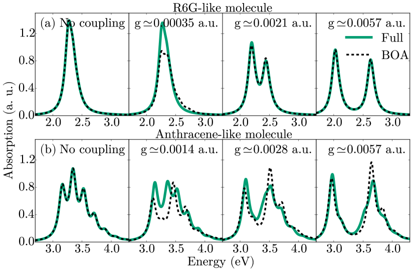
Figure 6: Absorption cross section of two molecules driven coherently, calculated using the full Hamiltonian without approximation (solid green lines) and within the BOA (dashed black lines). Results are shown for the (a) R6G-like and (b) anthracene-like model molecules, for several values of the coupling strength $g$. The values of $g$ are scaled by $1/\sqrt{2}$ with respect to the single-molecule case (Fig. 4) in order to obtain the same total Rabi frequency $\Omega_{R}$.

We first address the applicability of the BOA, which breaks down when two PES are close in energy, for the case of two molecules. Within the single-excitation subspace (which determines the linear properties of the system, such as absorption), there are now a range of (avoided) crossings. They occur when i) all three surfaces approach each other $E_{gg1}\approx E_{ge0}\approx E_{eg0}$, ii) the photonically excited PES is close to only one of the electronically excited PES, $E_{gg1}\approx E_{ge0}$ or $E_{gg1}\approx E_{eg0}$, or iii) only the two electronically excited states cross, $E_{ge0}\approx E_{eg0}$. Case i) corresponds to the JC model at zero detuning, giving the two polaritonic PES at energy shifts of $\pm\Omega_{R}/2$, and an additional dark state that is unshifted from the bare-molecule case. The BOA in this region is thus valid for similar conditions as in the single-molecule case, although the PES separation is reduced by half due to the additional dark-state surface. Case ii) corresponds exactly to the single-molecule case, with the second molecule acting as a “spectator” that only induces additional energy shifts. The BOA should thus again be valid for similar conditions as with a single-molecule, albeit with the coupling reduced by $1/\sqrt{2}$ for a fixed total Rabi splitting. Finally, case iii) presents the biggest challenge, as the two electronically excited PES, $E_{eg0}$ and $E_{ge0}$, are not directly coupled, but only split indirectly through coupling to the photonically excited surface $E_{gg1}$. The splitting between the two surfaces is thus small for large detuning, $\Delta E\approx(gd)^{2}/4(E_{gg1}-E_{eg0})$. This is clearly observed in Fig. 5b along the line $R_{1}=R_{2}$, where the dark state PES almost touches the upper polariton PES for small $R$s and the lower polariton PES for large $R$s.

The discussion above implies that for almost any coupling strength, there will be regions in the nuclear configuration space $R_{1},R_{2}$ where the BOA breaks down. However, not all parts of the PES are visited by the nuclei during a given physical process. To explicitly check the BOA in the subspace relevant for polaritonic physics, in Fig. 6 we thus again compare the absorption with that obtained by a full diagonalization of the Hamiltonian Eq. (missing) 8. Compared to the single-molecule case, many more molecular levels are present in the system, leading to small changes in the absorption spectra compared to the single-molecule case. In order to properly compare the results, we take into account the $\sqrt{N}$ scaling of the total Rabi frequency and reduce the coupling strengths by $\sqrt{2}$ to produce the same total splitting. The BOA is shown to again become valid for large enough coupling, but the minimum coupling required is increased compared to that for a single molecule. In the common case of slow nuclear motion, as for our R6G-like model in Fig. 6a, the BOA already is valid for relatively small Rabi splitting of $\Omega_{R}\approx 250$ eV. However, in the anthracene-like case of very fast vibrational motion, Fig. 6b, the BOA still does not give perfect agreement with the full model for $g=0.0057$ a.u. ($\Omega_{R}\approx 600$ meV), and agreement is only reached at roughly twice that value.

Having established the validity of the BOA for many relevant cases and Rabi splittings comparable to experimental values, we now discuss the implications of collective strong coupling for the internal molecular (nuclear) dynamics. Note that this question can by design not be addressed within the JC model, where emitters are two-level systems without any internal degrees of freedom. In contrast, the BOA provides a straightforward approach to this problem. Any two-dimensional PES can be decomposed into a sum of independent single-molecule potentials, plus a remainder that describes the coupling between the nuclear motion of the molecules,

$$E(R_{1},R_{2})=E_{1}(R_{1})+E_{2}(R_{2})+E_{12}(R_{1},R_{2}).$$ (10)

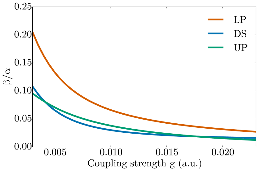
Figure 7: Coupling between nuclear motion in different molecules for the lower (LP) and upper polariton (UP) and dark-state (DS) PES. Results are shown as the ratio $\beta/\alpha$ between the prefactors of the offdiagonal $R_{1}R_{2}$ and diagonal $R_{i}^{2}$ terms in Eq. (missing) 11, for the R6G-like model molecule.

The nuclear motion of two molecules is independent if and only if the coupled part $E_{12}(R_{1},R_{2})$ is identically zero. In order to quantify this coupling, we expand each of the coupled PES in the single-excitation subspace around its minimum $(R_{1}^{0},R_{2}^{0})$, giving

$$E(R_{1},R_{2})\approx E_{0}+\alpha\,\delta R_{1}^{2}+\alpha\,\delta R_{2}^{2}+\beta\,\delta R_{1}\delta R_{2},$$ (11)

with $E_{0}=E(R_{1}^{0},R_{2}^{0})$ and $\delta R_{i}=R_{i}-R_{i}^{0}$. Note that due to symmetry under the exchange $R_{1}\leftrightarrow R_{2}$, the prefactor $\alpha$ is the same for $\delta R_{1}^{2}$ and $\delta R_{2}^{2}$. As can be seen in Fig. 7, both the polariton and even the dark state PES show significant coupling of the nuclear degrees of freedom, with values of $\beta/\alpha$ on the order of a few percent for values of $g\lesssim 0.01$ a.u. giving realistic Rabi splittings of $\lesssim 1$ eV (see Fig. 6). Interestingly, the coupling is much larger for the lower polariton state than for either the upper polariton or the dark state, and decreases with increasing $g$ for all three PES. We therefore conclude that even dark states that have negligible mixing with photonic modes are affected by strong coupling, in the sense that the nuclear degrees of freedom of separate molecules behave like coupled harmonic oscillators, and their motion becomes correlated. This implies that, e.g., local excitation of nuclear motion within one molecule could affect the nuclear motion in another, spatially separated molecule, even when no photon is ever present in the system. Note that these results apply within the singly-excited subspace, i.e., the coupled nuclear motion is only observed when electronic excitation is present, not in the ground state. In the next section, we discuss which modifications of the ground state properties could be observed in the ultrastrong coupling regime.

IV Ultrastrong coupling and ground state modifications

Up to now, we focused on the molecular properties in the singly excited subspace, which are probed in linear response measurements such as absorption and transmission, and where the effect of strong coupling is immediately apparent. However, when the Rabi frequency, i.e., the energy exchange rate between the molecules and the photonic mode, becomes significant compared to the frequencies of these two modes, the so-called ultra-strong coupling regime is entered De Liberato et al. (2007); Carusotto and Ciuti (2013). In this regime, the rotating wave approximation for the emitter-light interaction (under which the number of excitations is conserved) becomes invalid. In our approach, the rotating wave approximation is not used, and we can thus naturally explore the ultrastrong coupling regime. One of its most intriguing predictions is that even the ground-state properties of the system should be significantly modified. For example, the ground state is shifted in energy and acquires a photonic component, such that a number of virtual photons are present in the system even without any external excitations. This raises the question of how the internal degrees of freedom of organic molecules are affected when this regime is entered.

The BOA is well-suited to explore this regime. In contrast to the singly-excited subspace, where narrow avoided crossings can affect its validity, the ground-state PES is energetically well-separated from all other PES. This remains true even under ultrastrong coupling, and consequently the BOA is valid for all coupling strengths. The ground state potential energy surface $E_{g}(R)$ is coupled to the doubly excited surface $E_{e}(R)+\omega_{c}$ (cf. Eq. (missing) 9a), with the strongly coupled ground state PES given to lowest order by $E_{g}^{SC}(R)\approx E_{g}(R)-\frac{g^{2}\mu_{eg}^{2}(R)}{E_{e}(R)+\omega_{c}-E_{g}(R)}+O(g^{4})$. Ground state properties such as the bond length are determined by the shape of the PES. The largest modification can thus be expected when the $R$-dependence of the ground and excited PES is as different as possible. This occurs for large electron-phonon coupling, i.e., a large value of $\Delta R$, such as in our anthracene-like molecule. For a coupling strength of $g=0.016$ a.u., corresponding to a Rabi splitting of $\Omega_{R}\approx 1.2$ eV in absorption, we obtain a shift in the ground state bond length of $\Delta R_{0}\approx 0.84$ mÅ$=84$ fm. While small, such a change in bond length could be detectable using X-ray absorption fine structure spectroscopy or X-ray crystallography, which can obtain few- or even sub-femtometer precision for measuring bond length shifts König et al. (2012); Kozina et al. (2014).

However, the previous paragraph only applies for a single molecule under strong coupling. Repeating the calculation using two molecules and taking into account the reduced single-molecule coupling strength (for fixed Rabi splitting, $\Omega_{R}\propto\sqrt{N}g$) reveals a reduction of the bond-length change by a factor of two, $\Delta R_{0}^{2mol}\approx 0.42$ mÅ. This is confirmed by using a similar analytical model as presented in appendix A, in which the bare-molecule potential energy surfaces are approximated as harmonic oscillators. Due to the simple analytical structure, perturbation theory can be applied to obtain results for arbitrary numbers of molecules, and the change in ground-state bond length is found to be proportional to the squared single-molecule coupling $g^{2}$, not to the squared collective Rabi frequency $\Omega_{R}^{2}$. We note that in contrast, the ground-state energy shift is indeed determined by the collective coupling strength, $\Delta E_{0}\propto\Omega_{R}^{2}$. In realistic experimental configurations involving large numbers of molecules, the change in ground state bond length is thus expected to be minuscule and extremely challenging to measure. This demonstrates that the influence of strong coupling on any specific observable is not immediately obvious, and has to be checked case by case. For some properties, the molecules will behave as if they feel the full collective coupling $\Omega_{R}$, while for others, they will only show the change induced by the single-molecule coupling $g$.

We thus check another observable, and ask whether the ground state will show correlated nuclear motion between distant molecules, as observed in the dark state surface. This can again be quantified using the expansion of the PES in Eq. (missing) 11. Doing so reveals a very small coupling parameter $\beta$ that to lowest order is proportional to $g^{4}/\omega_{c}^{5}$ (close to zero detuning, $\omega_{c}\sim E_{e}(R)-E_{g}(R)$). This corresponds to an even higher-order correction than the already small energy or bond-length shifts. Furthermore, like the bond-length shift, it depends on the single-molecule coupling instead of the collective coupling strength. We can thus conclude that in contrast to the excited states, the ground-state nuclear motion of the molecules does not become correlated even in the ultrastrong coupling limit.

V Conclusions & Outlook

We have presented a simple model that offers a new perspective on strong coupling with organic molecules. We have shown under which conditions the molecular properties under strong coupling can be understood by the modification of the potential energy surfaces determining nuclear dynamics under the Born-Oppenheimer approximation. In particular, we found that in many cases of experimental interest where the Rabi splitting is large, the BOA is applicable and provides an intuitive picture of the strongly coupled dynamics. However, we have also shown that for molecules with fast vibrational modes and large phonon-exciton couplings, the BOA can break down and a more involved picture is necessary. We furthermore demonstrated that the non-BO coupling terms between PES in this case are dominantly due to the change of character between light and matter excitations which can be obtained from simple few-level models without requiring knowledge of the electronic wavefunctions.

In addition, we have shown that under collective strong coupling involving more than one molecule, the nuclear dynamics of the molecules in electronic “dark states” that are only weakly coupled to the photonic mode are nonetheless affected by the formation of strong coupling. In particular, we find that the dark state PES describes coupling between the nuclear degrees of freedom of the different molecules.

Finally, we investigated the change of the ground state properties under ultrastrong coupling, where the Rabi splitting becomes a significant fraction of the transition energy. Using our numerical calculations and a simple analytical model, we showed that while the ground-state energy shift is affected by the collective Rabi frequency (which is enhanced by $\sqrt{N}$ for $N$ molecules), other properties such as the ground-state bond length depend on the single-molecule coupling strength and are not significantly affected for experimentally realistic parameters.

Our results also lay the groundwork for a further in-depth exploration of the modification of molecular properties under strong coupling. In particular, they provide a simple picture that can be used to understand the modification of chemical reactions, e.g., by lowering a potential barrier along a reaction coordinate. There are also a number of obvious extensions of the simple model presented here that will be explored in the future. These include more realistic models of organic molecules using more degrees of freedom (for example, employing the PES obtained using quantum chemistry packages), and the inclusion of incoherent processes such as decay and decoherence. We note that there has been some recent progress on combining QED with density functional theory Tokatly (2013); Ruggenthaler et al. (2014), which could provide complementary information to the model presented here.

Appendix A Model for non-Born-Oppenheimer corrections

In this appendix, we derive an analytical model for the non-Born-Oppenheimer corrections $\hat{C}_{n}^{kk^{\prime}}$ under molecular strong coupling, for a single molecule. We treat the two PES in the single-excitation subspace, $E_{g}(R)+\omega_{c}$ and $E_{e}(R)$, coupled by the term $g\mu_{eg}(R)$. This leads to a $2\times 2$ BO Hamiltonian of the form

$$\hat{H}(R)=\begin{pmatrix}E_{g}(R)+\omega_{c}&g\mu_{eg}(R)\\ g\mu_{eg}(R)&E_{e}(R)\end{pmatrix},$$ (12)

which can be easily diagonalized to obtain polariton eigenstates $|+\rangle=\cos\theta|g1\rangle+\sin\theta|e0\rangle$ and $|-\rangle=\sin\theta|g1\rangle-\cos\theta|e0\rangle$, where $|an\rangle$ is short for $|\phi_{a}(x;R),n\rangle$, and

$$\tan 2\theta=\frac{2h(R)}{\delta E(R)}\,,$$ (13)

where we defined $\delta E(R)=E_{g}(R)+\omega_{c}-E_{e}(R)$ and $h(R)=g\mu_{eg}(R)$. Using $E_{\mathrm{avg}}(R)=\frac{E_{g}(R)+\omega_{c}+E_{e}(R)}{2}$, the eigenenergies are given by

$$E_{\pm}(R)=E_{\mathrm{avg}}(R)\pm\frac{1}{2}\sqrt{4h^{2}(R)+\delta E(R)^{2}}\,.$$ (14)

We can now evaluate the non-Born-Oppenheimer coupling terms $\hat{C}_{n}^{kk^{\prime}}=\langle k|\hat{T}_{n}|k^{\prime}\rangle+\langle k|\frac{\hat{P}}{2M}|k^{\prime}\rangle\hat{P}$ within this model, using a series of approximations to obtain simple analytical results. First, we linearize $\delta E(R)\approx a_{0}(R-R_{c})$ around the point of intersection between the two PES, where $E_{g}(R_{c})+\omega_{c}=E_{e}(R_{c})$. Second, in the spirit of the Franck-Condon approximation, we assume that the dipole coupling is constant over the range of relevant $R$-values, and set $h(R)=h_{0}$. Following the same idea, we additionally assume that the electronic wave functions do not change significantly with $R$, i.e., $\frac{\partial}{\partial R}|\phi_{a}(x;R)\rangle\approx 0$. This implies that the change in the polaritonic eigenfunctions $|\pm\rangle$ close to the avoided crossing at $R_{c}$ is mostly due to the switchover between the two uncoupled surfaces, i.e., the change in $\theta(R)$, not because of an intrinsic change of electronic state with $R$. With these approximations, the correction terms become

$$\langle-|\hat{P}|+\rangle =\frac{-ia_{0}h_{0}}{4h_{0}^{2}+a_{0}^{2}(R-R_{c})^{2}},$$ (15a)

$$\langle-|\hat{P}^{2}|+\rangle =\frac{2a_{0}^{3}h_{0}(R-R_{c})}{(4h_{0}^{2}+a_{0}^{2}(R-R_{c})^{2})^{2}},$$ (15b)

$$\langle\pm|\hat{P}^{2}|\pm\rangle =\frac{a_{0}^{2}h_{0}^{2}}{(4h_{0}^{2}+a_{0}^{2}(R-R_{c})^{2})^{2}},$$ (15c)

with the diagonal terms $\langle\pm|\hat{P}|\pm\rangle$ identically zero. Note that diagonal terms only correspond to energy shifts and do not induce additional transitions Tully (2000). The non-Born-Oppenheimer coupling between the polariton surfaces has a Lorentzian shape around the avoided crossing, and as expected only becomes non-negligible close to it.

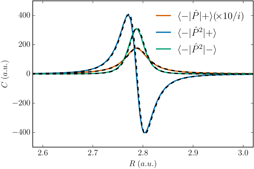
Figure 8: Non-Born-Oppenheimer correction terms coupling the “lower polariton” and “upper polariton” PES for a single anthracene-like model molecule for a coupling strength of $g=0.002$ a.u.. Solid colored lines: results from a full numerical calculation. Dashed black lines: results from the model Eq. (missing) 15. Note that while all results are given in atomic units, the units of the $\hat{P}$ and $\hat{P}^{2}$ terms are not identical, and thus not directly comparable.

As shown in Fig. 8, the non-Born-Oppenheimer corrections obtained from this simple model agree almost perfectly with those obtained from the full numerical calculation for our anthracene-like model molecule. The only molecule-specific information entering the model are the PES of the uncoupled molecule and the dipole moment between the coupled surfaces. Specifically, the electronic wave functions are never used here, and their derivative as a function of the nuclear coordinates is not required. This implies that this model could be used to obtain accurate non-BO corrections that describe the transitions between potential surfaces even when the full electronic wave functions of a molecule are not available (e.g., in DFT calculations). The dynamics of the molecule could thus be fully recovered within a potential energy surface picture even when the BOA per se is not applicable.

We now exploit this model to derive a condition for when the BOA becomes applicable, i.e., when the non-BO terms become negligible. We approximate the bare molecular potential energy surfaces as two harmonic oscillators with the same vibrational frequency $\omega_{vib}$, but with an offset in energy and equilibrium position,

$$E_{g}(R) \approx\frac{M\omega_{vib}^{2}}{2}R^{2},$$ (16)

$$E_{e}(R) \approx\frac{M\omega_{vib}^{2}}{2}(R-\Delta R)^{2}+\Delta E,$$ (17)

where without loss of generality, we have chosen the origin in $R$ and $E$ at the minimum of $E_{g}(R)$. Note that this model exactly results from the common approximation of linear coupling between a single electronic excitation and a bosonic vibrational mode Leggett et al. (1987); Coalson et al. (1994). Within this model, $\delta E(R)=E_{g}(R)+\omega_{c}-E_{e}(R)=a_{0}(R-R_{c})$ is already exactly linear, i.e., the linearization of the energy difference performed above is not an approximation. The constants are given by $a_{0}=M\omega_{vib}^{2}\Delta R$ and $R_{c}=\frac{\Delta R}{2}+\frac{\Delta E-\omega_{c}}{a_{0}}$. The maximum value of $|\langle+|\frac{\hat{P}}{2M}|-\rangle|$, reached at $R=R_{c}$, is given by $\Delta R\omega_{vib}^{2}/(8h_{0})$. Comparing this with the energy splitting at that point, $E_{+}(R_{c})-E_{-}(R_{c})=2h_{0}$, gives the condition that $\Delta R\omega_{vib}^{2}/(16h_{0}^{2})$ must be small compared to the momentum of the respective nuclear wavefunction (due to the additional $\hat{P}$ operating on the nuclear wave function). The off-diagonal terms from $\langle-|\hat{P}^{2}|+\rangle$ reach a maximum value (again relative to the detuning) of $M\Delta R^{2}\omega_{vib}^{4}/(25\sqrt{5}h_{0}^{3})$ at $R=R_{c}+h_{0}/(M\Delta R\omega_{vib}^{2})$.

References

- Thompson et al. (1992) R. J. Thompson, G. Rempe, and H. J. Kimble, “Observation of normal-mode splitting for an atom in an optical cavity,” Phys. Rev. Lett. 68, 1132–1135 (1992).
- Weisbuch et al. (1992) C. Weisbuch, M. Nishioka, A. Ishikawa, and Y. Arakawa, “Observation of the coupled exciton-photon mode splitting in a semiconductor quantum microcavity,” Phys. Rev. Lett. 69, 3314–3317 (1992).
- Kasprzak et al. (2006) J. Kasprzak, M. Richard, S. Kundermann, A. Baas, P. Jeambrun, J. M. J. Keeling, F. M. Marchetti, M. H. Szymańska, R. André, J. L. Staehli, V. Savona, P. B. Littlewood, B. Deveaud, and Le Si Dang, “Bose-Einstein condensation of exciton polaritons,” Nature 443, 409–14 (2006).
- Balili et al. (2007) R. Balili, V. Hartwell, D. Snoke, L. Pfeiffer, and K. West, “Bose-Einstein condensation of microcavity polaritons in a trap,” Science 316, 1007–10 (2007).
- Kéna-Cohen and Forrest (2010) S. Kéna-Cohen and S. R. Forrest, “Room-temperature polariton lasing in an organic single-crystal microcavity,” Nat. Phot. 4, 371–375 (2010).
- Plumhof et al. (2014) Johannes D. Plumhof, Thilo Stöferle, Lijian Mai, Ullrich Scherf, and Rainer F. Mahrt, “Room-temperature Bose-Einstein condensation of cavity exciton-polaritons in a polymer.” Nat. Mater. 13, 247–52 (2014).
- Daskalakis et al. (2014) K. S. Daskalakis, S. A. Maier, R. Murray, and S. Kéna-Cohen, “Nonlinear interactions in an organic polariton condensate.” Nat. Mater. 13, 271–8 (2014).
- Lidzey et al. (1998) D. G. Lidzey, D. D. C. Bradley, M. S. Skolnick, T. Virgili, S. Walker, and D. M. Whittaker, “Strong exciton-photon coupling in an organic semiconductor microcavity,” Nature 395, 53–55 (1998).
- Schwartz et al. (2011) T. Schwartz, J. A. Hutchison, C. Genet, and T. W. Ebbesen, “Reversible Switching of Ultrastrong Light-Molecule Coupling,” Phys. Rev. Lett. 106, 196405 (2011).
- Kéna-Cohen et al. (2013) Stéphane Kéna-Cohen, Stefan A. Maier, and Donal D. C. Bradley, “Ultrastrongly Coupled Exciton-Polaritons in Metal-Clad Organic Semiconductor Microcavities,” Adv. Opt. Mater. 1, 827–833 (2013).
- Törmä and Barnes (2015) P. Törmä and W. L. Barnes, “Strong coupling between surface plasmon polaritons and emitters: a review,” Rep. Prog. Phys. 78, 013901 (2015).
- Kéna-Cohen et al. (2008) S. Kéna-Cohen, M. Davanço, and S. R. Forrest, “Strong Exciton-Photon Coupling in an Organic Single Crystal Microcavity,” Phys. Rev. Lett. 101, 116401 (2008).
- Bellessa et al. (2004) J. Bellessa, C. Bonnand, J. C. Plenet, and J. Mugnier, “Strong Coupling between Surface Plasmons and Excitons in an Organic Semiconductor,” Phys. Rev. Lett. 93, 036404 (2004).
- Dintinger et al. (2005) J. Dintinger, S. Klein, F. Bustos, W. L. Barnes, and T. W. Ebbesen, “Strong coupling between surface plasmon-polaritons and organic molecules in subwavelength hole arrays,” Phys. Rev. B 71, 035424 (2005).
- Hakala et al. (2009) T. K. Hakala, J. J. Toppari, A. Kuzyk, M. Pettersson, H. Tikkanen, H. Kunttu, and P. Törmä, “Vacuum Rabi Splitting and Strong-Coupling Dynamics for Surface-Plasmon Polaritons and Rhodamine 6G Molecules,” Phys. Rev. Lett. 103, 053602 (2009).
- Vasa et al. (2010) P. Vasa, R. Pomraenke, G. Cirmi, E. De Re, W. Wang, S. Schwieger, D. Leipold, E. Runge, G. Cerullo, and C. Lienau, “Ultrafast manipulation of strong coupling in metal-molecular aggregate hybrid nanostructures,” ACS Nano 4, 7559–65 (2010).
- Rodriguez et al. (2013) S. R. K. Rodriguez, J. Feist, M. A. Verschuuren, F. J. García Vidal, and J. Gómez Rivas, “Thermalization and Cooling of Plasmon-Exciton Polaritons: Towards Quantum Condensation,” Phys. Rev. Lett. 111, 166802 (2013).
- Väkeväinen et al. (2014) A. I. Väkeväinen, R. J. Moerland, H. T. Rekola, A.-P. Eskelinen, J.-P. Martikainen, D.-H. Kim, and P. Törmä, “Plasmonic Surface Lattice Resonances at the Strong Coupling Regime,” Nano Lett. 14, 1721–7 (2014).
- Baudrion et al. (2013) Anne Laure Baudrion, Antoine Perron, Alessandro Veltri, Alexandre Bouhelier, Pierre Michel Adam, and Renaud Bachelot, “Reversible strong coupling in silver nanoparticle arrays using photochromic molecules,” Nano Lett. 13, 282–286 (2013).
- Zengin et al. (2015) Gülis Zengin, Martin Wersäll, Sara Nilsson, Tomasz J. Antosiewicz, Mikael Käll, and Timur Shegai, “Realizing Strong Light-Matter Interactions between Single-Nanoparticle Plasmons and Molecular Excitons at Ambient Conditions,” Phys. Rev. Lett. 114, 157401 (2015).
- Hutchison et al. (2012) James A. Hutchison, Tal Schwartz, Cyriaque Genet, Eloïse Devaux, and Thomas W. Ebbesen, “Modifying Chemical Landscapes by Coupling to Vacuum Fields,” Angew. Chemie 124, 1624–1628 (2012).
- Hutchison et al. (2013) James A. Hutchison, Andrea Liscio, Tal Schwartz, Antoine Canaguier-Durand, Cyriaque Genet, Vincenzo Palermo, Paolo Samorì, and Thomas W. Ebbesen, “Tuning the work-function via strong coupling,” Adv. Mater. 25, 2481–5 (2013).
- Wang et al. (2014) Shaojun Wang, Arkadiusz Mika, James A. Hutchison, Cyriaque Genet, Abdelaziz Jouaiti, Mir Wais Hosseini, and Thomas W. Ebbesen, “Phase transition of a perovskite strongly coupled to the vacuum field,” Nanoscale 6, 7243–8 (2014).
- Carusotto and Ciuti (2013) Iacopo Carusotto and Cristiano Ciuti, “Quantum fluids of light,” Rev. Mod. Phys. 85, 299–366 (2013).
- Michetti et al. (2015) Paolo Michetti, Leonardo Mazza, and Giuseppe C. La Rocca, “Strongly Coupled Organic Microcavities,” in Organic Nanophotonics, Nano-Optics and Nanophotonics, edited by Yong Sheng Zhao (Springer, Berlin, Heidelberg, 2015) pp. 39–68.
- González-Tudela et al. (2013) A. González-Tudela, P. A. Huidobro, L. Martín-Moreno, C. Tejedor, and F. J. García-Vidal, “Theory of Strong Coupling between Quantum Emitters and Propagating Surface Plasmons,” Phys. Rev. Lett. 110, 126801 (2013).
- Mazza et al. (2013) L. Mazza, S. Kéna-Cohen, P. Michetti, and G. C. La Rocca, “Microscopic theory of polariton lasing via vibronically assisted scattering,” Phys. Rev. B 88, 075321 (2013).
- Ćwik et al. (2014) Justyna A. Ćwik, Sahinur Reja, Peter B. Littlewood, and Jonathan Keeling, “Polariton condensation with saturable molecules dressed by vibrational modes,” EPL 105, 47009 (2014).
- Born and Oppenheimer (1927) M. Born and R. Oppenheimer, “Zur Quantentheorie der Molekeln,” Ann. Phys. 20, 457–484 (1927).
- Tully (2000) John C. Tully, “Perspective on "Zur Quantentheorie der Molekeln",” Theor. Chem. Acc. 103, 173–176 (2000).
- Houdré et al. (1996) R. Houdré, R. P. Stanley, and M. Ilegems, “Vacuum-field Rabi splitting in the presence of inhomogeneous broadening: Resolution of a homogeneous linewidth in an inhomogeneously broadened system,” Phys. Rev. A 53, 2711–2715 (1996).
- Agranovich et al. (2011) V. M. Agranovich, Yu. N. Gartstein, and M. Litinskaya, “Hybrid resonant organic-inorganic nanostructures for optoelectronic applications,” Chem. Rev. 111, 5179–5214 (2011).
- De Liberato et al. (2007) Simone De Liberato, Cristiano Ciuti, and Iacopo Carusotto, “Quantum Vacuum Radiation Spectra from a Semiconductor Microcavity with a Time-Modulated Vacuum Rabi Frequency,” Phys. Rev. Lett. 98, 103602 (2007).
- George et al. (2015) Jino George, Shaojun Wang, Thibault Chervy, Antoine Canaguier-Durand, Gael Schaeffer, Jean-Marie Lehn, James A. Hutchison, Cyriaque Genet, and Thomas W. Ebbesen, “Ultra-strong coupling of molecular materials: spectroscopy and dynamics,” Faraday Discuss. 178, 281–294 (2015).
- May and Kühn (2011) Volkhard May and Oliver Kühn, Charge and Energy Transfer Dynamics in Molecular Systems (Wiley-VCH Verlag GmbH & Co. KGaA, Weinheim, Germany, 2011).
- Kim et al. (2015) Myung-Ki Kim, Hongchul Sim, Seung Ju Yoon, Su-Hyun Gong, Chi Won Ahn, Yong-Hoon Cho, and Yong-Hee Lee, “Squeezing Photons into a Point-Like Space,” Nano Lett. (2015), 10.1021/acs.nanolett.5b01204.
- Moll et al. (1995) Johannes Moll, Siegfried Daehne, James R. Durrant, and Douwe A. Wiersma, “Optical dynamics of excitons in J aggregates of a carbocyanine dye,” J. Chem. Phys. 102, 6362 (1995).
- Rescigno and McKoy (1975) Thomas N. Rescigno and Vincent McKoy, “Rigorous method for computing photoabsorption cross sections from a basis-set expansion,” Phys. Rev. A 12, 522–525 (1975).
- Bonin and Kresin (1997) Keith D. Bonin and Vitaly V. Kresin, Electric-Dipole Polarizabilities Of Atoms, Molecules, And Clusters (World Scientific Publishing Co. Pte. Ltd., 1997).
- Shimanouchi (1972) Takehiko Shimanouchi, “Tables of Molecular Vibrational Frequencies. Consolidated Volume I,” NSRDS-NBS 39, 161p. (1972).
- Dicke (1954) R. Dicke, “Coherence in Spontaneous Radiation Processes,” Phys. Rev. 93, 99–110 (1954).
- Jaynes and Cummings (1963) E. T. Jaynes and F. W. Cummings, “Comparison of quantum and semiclassical radiation theories with application to the beam maser,” Proc. IEEE 51, 89–109 (1963).
- Tavis and Cummings (1967) M. Tavis and F. W. Cummings, “The exact solution of N two level systems interacting with a single mode, quantized radiation field,” Phys. Lett. A 25, 714–715 (1967).
- König et al. (2012) Christian F. J. König, Jeroen A. van Bokhoven, Tilman J. Schildhauer, and Maarten Nachtegaal, “Quantitative analysis of modulated excitation X-ray absorption spectra: Enhanced precision of EXAFS fitting,” J. Phys. Chem. C 116, 19857–19866 (2012).
- Kozina et al. (2014) M. Kozina, T. Hu, J. S. Wittenberg, E. Szilagyi, M. Trigo, T. A. Miller, C. Uher, A. Damodaran, L. Martin, A. Mehta, J. Corbett, J. Safranek, D. A. Reis, and A. M. Lindenberg, “Measurement of transient atomic displacements in thin films with picosecond and femtometer resolution,” Struct. Dyn. 1, 034301 (2014).
- Tokatly (2013) I. V. Tokatly, “Time-dependent density functional theory for many-electron systems interacting with cavity photons,” Phys. Rev. Lett. 110, 233001 (2013).
- Ruggenthaler et al. (2014) Michael Ruggenthaler, Johannes Flick, Camilla Pellegrini, Heiko Appel, Ilya V. Tokatly, and Angel Rubio, “Quantum-electrodynamical density-functional theory: Bridging quantum optics and electronic-structure theory,” Phys. Rev. A 90, 012508 (2014).
- Leggett et al. (1987) A. J. Leggett, S. Chakravarty, A. T. Dorsey, Matthew P. A. Fisher, Anupam Garg, and W. Zwerger, “Dynamics of the dissipative two-state system,” Rev. Mod. Phys. 59, 1–85 (1987).
- Coalson et al. (1994) Rob D. Coalson, Deborah G. Evans, and Abraham Nitzan, “A nonequilibrium golden rule formula for electronic state populations in nonadiabatically coupled systems,” J. Chem. Phys. 101, 436 (1994).