Bilayer Plates: Model Reduction, $\Gamma$-Convergent Finite Element Approximation and Discrete Gradient Flow

Abstract.

The bending of bilayer plates is a mechanism which allows for large deformations via small externally induced lattice mismatches of the underlying materials. Its mathematical modeling, discussed herein, consists of a nonlinear fourth order problem with a pointwise isometry constraint. A discretization based on Kirchhoff quadrilaterals is devised and its $\Gamma$-convergence is proved. An iterative method that decreases the energy is proposed and its convergence to stationary configurations is investigated. Its performance, as well as reduced model capabilities, are explored via several insightful numerical experiments involving large (geometrically nonlinear) deformations.

1. Introduction

The derivation of dimensionally reduced mathematical models and their numerical treatment is a classical and challenging scientific branch within solid mechanics. Various models for describing the bending or membrane behavior of plates are available, either as linear models for the description of small displacements or nonlinear models when large deformations are considered; see [11]. The development of related numerical methods has mostly been concerned with the treatment of second order derivatives and avoiding various locking effects. The rigorous derivation of the geometrically nonlinear Kirchhoff model for the description of large bending deformations of plates from three-dimensional hyperelasticity in [14] has inspired various further results, e.g., discussing other energy regimes in [15], or the derivation of effective theories for prestressed multilayer materials in [21].

Bilayer plates consist of two films of different materials glued on top of each other. The materials react differently to thermal or electric stimuli, thereby changing their molecular lattices. This mismatch allows for the development of large deformations by simple heat or electric actuation. Classical applications of this effect include bimetal strips in thermostats, while modern applications use thermally and electrically induced bending effect to produce nanorolls, microgrippers, and nano-tubes; see [5, 18, 19, 22, 23]. Preventing undesirable effects such as dog-ears formation, as reported in [1, 24], motivates the mathematical prediction of bilayer bending patterns via numerical simulation. This requires having a model as simple as possible to be ameanable to numerical treatment and analysis, but sufficiently sophisticated to capture essential nonlinear geometric features associated with large bending deformations.

A two-dimensional mathematical model for the bending behavior of bilayers has been rigorously derived from three-dimensional hyperelasticity in [21]. It consists of a nonconvex minimization problem with nonlinear pointwise constraint. The energy functional involves second order derivatives of deformations associated with the second fundamental form of the mid-surface. The pointwise constraint enforces deformations to be isometries, i.e., that length and angle relations remain unchanged by the deformation as in the case of the bending of a piece of paper. A related numerical method has been devised and analyzed for single layer plates in [3, 4].

It is our goal to develop a reliable numerical method for the practical computation of large bilayer bending deformations. Our contributions in this paper are:

1. To present a formal dimension reduction model allowing for various effects not covered in the corresponding rigorous analysis in [20];

2. To propose a discretization of the mathematical model and prove its $\Gamma$-convergence as discretization parameters tend to zero;

3. To construct a gradient flow method to compute stationary configurations;

4. To carry out several numerical experiments to illustrate the performance of our numerical method and explore the nonlinear geometric effects captured by the mathematical model.

In the remainder of this introduction we discuss the mathematical model and our main ideas to deal with the ensuing strong nonlinearities.

Description of bilayer plates. We consider a geometrically nonlinear Kirchhoff plate model that allows for bending but not for stretching or shear. This selection is related to the choice of a particular energy scaling, namely that the elastic energy is proportional to the third power of the plate thickness $t$. Given a domain $\omega\subset\mathbb{R}^{2}$ that describes the middle surface of the plate, the model formally derived in Section 2 consists of minimizing the dimensionally reduced elastic energy

(1.1) $$E[{\bf y}]=\frac{1}{2}\int_{\omega}\big{|}H+Z\big{|}^{2}-\int_{\omega}{\bf f}\cdot{\bf y}$$

within the set of isometries ${\bf y}:\omega\to\mathbb{R}^{3}$, i.e., mappings satisfying the identities

(1.2) $$[\nabla{\bf y}]^{T}\nabla{\bf y}=I_{2}\qquad\Longleftrightarrow\qquad\partial_{i}{\bf y}\cdot\partial_{j}{\bf y}=\delta_{ij},\quad i,j=1,2,$$

in $\omega$ and with prescribed values ${\bf y}={\bf y}_{D}$ and $\nabla{\bf y}=\Phi_{D}$ on the Dirichlet portion $\partial_{D}\omega$ of the boundary $\partial\omega$. Hereafter, $I_{d}$ denotes the identity matrix in $\mathbb{R}^{d}$ for $d=2,3$, and $H$ stands for the second fundamental form of the surface $\gamma={\bf y}(\omega)$ parametrized by ${\bf y}$ with unit normal ${\bf\nu}$,

$$H_{i,j}={\bf\nu}\cdot\partial_{i}\partial_{j}{\bf y},\quad{\bf\nu}=\partial_{1}{\bf y}\times\partial_{2}{\bf y}.$$

The symmetric matrix $Z$ is given and can be viewed as a spontaneous curvature so that in the absence of body forces ${\bf f}$ the plate is already pre-stressed. Given the identity for isometries

$$|H|^{2}=|D^{2}{\bf y}|^{2},$$

we rewrite the energy $E[{\bf y}]$ in (1.1) as follows:

(1.3) $$\widetilde{E}[{\bf y}]:=\frac{1}{2}\int_{\omega}|D^{2}{\bf y}|^{2}+\sum_{i,j=1}^{2}\int_{\omega}\partial_{i}\partial_{j}{\bf y}\cdot\Big{(}\frac{\partial_{1}{\bf y}}{|\partial_{1}{\bf y}|}\times\frac{\partial_{2}{\bf y}}{|\partial_{2}{\bf y}|}\Big{)}Z_{ij}+\frac{1}{2}\int_{\omega}|Z|^{2}-\int_{\omega}{\bf f}\cdot{\bf y}.$$

It is tempting to simplify this expression further because $|\partial_{i}{\bf y}|=1$, $i=1,2$, for isometries. However, we refrain from doing so for stability purposes anticipating that the isometry constraint will be later relaxed numerically. In particular, the normalization will enable us to prove various bounds for the variational derivative of the energy. In fact, notice that the energy $\widetilde{E}[{\bf y}]$ is finite for ${\bf y}\in H^{2}(\omega)^{3}\cap W^{1}_{\infty}(\omega)^{3}$ such that $|\partial_{i}{\bf y}|\geq 1$, $i=1,2$, as well as ${\bf f}\in L^{2}(\omega)^{3}$ and $Z\in L^{2}(\omega)^{2\times 2}$. The condition $|\partial_{i}{\bf y}|\geq 1$, $i=1,2$, will play a crucial role throughout this paper. We encode boundary conditions and the isometry constraint in the set of admissible deformations

(1.4) $$\mathcal{A}:=\big{\{}{\bf y}\in H^{2}(\omega)^{3}:{\bf y}|_{\partial_{D}\omega}={\bf y}_{D},\nabla{\bf y}|_{\partial_{D}\omega}=\Phi_{D},[\nabla{\bf y}]^{T}\nabla{\bf y}=I_{2}~{}\text{a.e. in }\omega\big{\}}$$

and define the tangent space of $\mathcal{A}$ at a point ${\bf y}\in\mathcal{A}$ via

(1.5) $$\mathcal{F}[{\bf y}]:=\big{\{}{\bf w}\in H^{2}(\omega)^{3}:{\bf w}|_{\partial_{D}\omega}=0,\nabla{\bf w}|_{\partial_{D}\omega}=0,\ [\nabla{\bf w}]^{T}\nabla{\bf y}+[\nabla{\bf y}]^{T}\nabla{\bf w}=0~{}\text{a.e. in }\omega\big{\}}.$$

Note that it is always possible to extend the functional $\widetilde{E}$ to $H^{1}(\omega)^{3}$ as follows:

$$\widetilde{E}[{\bf y}]:=+\infty,\qquad{\bf y}\in H^{1}(\omega)^{3}\setminus\mathcal{A}.$$

Minimizing movements. To find stationary points of $\widetilde{E}$ in $\mathcal{A}$, we propose a gradient flow in $H^{2}(\omega)$, i.e. according to the $H^{2}$-scalar product: if $s\in(0,\infty)$ is a pseudo-time, we formally seek a family ${\bf y}\in L^{2}(0,\infty;\mathcal{A})$ with $\partial_{s}{\bf y}(s)\in\mathcal{F}[{\bf y}(s)]$ for $s\in(0,\infty)$ and

$$\int_{\omega}D^{2}\big{(}\partial_{s}{\bf y}(s)\big{)}:D^{2}{\bf w}=-\delta\widetilde{E}[{\bf y}(s),{\bf w}]\qquad\forall{\bf w}\in\mathcal{F}[{\bf y}(s)].$$

The expression $\delta\widetilde{E}[{\bf y},{\bf w}]$ stands for the variational derivative of $\widetilde{E}$ at ${\bf y}\in\mathcal{A}$ in the direction ${\bf w}\in\mathcal{F}[{\bf y}(s)]$, which we make explicit below. We note that upon taking ${\bf w}=\partial_{s}{\bf y}(s)\in\mathcal{F}[{\bf y}(s)]$, we obtain formally

$$\frac{d}{ds}\widetilde{E}[{\bf y}(s)]=-\int_{\omega}\big{|}D^{2}\big{(}\partial_{s}{\bf y}(s)\big{)}\big{|}^{2}\leq 0;$$

the energy thus decreases along trajectories. The formal gradient flow is highly nonlinear and requires an appropriate interpretation. We adopt the concept of minimizing movements and consider an implicit first order time-discretization of the $H^{2}$-gradient flow via successive minimization of

$${\bf y}\mapsto\frac{1}{2\tau}\|D^{2}({\bf y}-{\bf y}^{k})\|_{L^{2}(\omega)}^{2}+\widetilde{E}[{\bf y}]$$

in the set of all ${\bf y}\in\mathcal{A}$ to determine ${\bf y}^{k+1}$. Our motivation for the use of the $H^{2}$ metric to define the gradient flow is threefold. First, it simplifies the implementation since it leads to the same system matrix as the main part of the bilinear form associated with the bending energy (1.3). Second, it is sufficiently strong to provide control over discrete time derivatives and discretization errors, such as the isometry constraint, without imposing severe step size restrictions. Third, it may be regarded as a damping term modeling the deceleration of a bilayer within a viscous fluid, which in turn gives some physical interpretation. Since the nonlinear isometry constraint is treated exactly, this nonconvex minimization problem is of limited practical value. We thus propose instead a linearization of the isometry constraint which yields a practical scheme.

Algorithm 1 (minimizing movement).

Let $\tau>0$ be the time-step size and set $k=0$. Choose ${\bf y}^{0}\in\mathcal{A}$. Compute ${\bf v}^{k+1}\in\mathcal{F}[{\bf y}^{k}]$ which is minimal for the functional

$${\bf v}\mapsto\frac{\tau}{2}\|D^{2}{\bf v}\|_{L^{2}(\omega)}^{2}+\widetilde{E}[{\bf y}^{k}+\tau{\bf v}],$$

set ${\bf y}^{k+1}={\bf y}^{k}+\tau{\bf v}^{k+1}$, increase $k\to k+1$ and repeat.

The linearized isometry condition included in the set $\mathcal{F}[{\bf y}^{k}]$ implies that for every admissible vector field ${\bf v}\in\mathcal{F}[{\bf y}^{k}]$ we have that the constraint residual of the corresponding update ${\bf y}^{k}+\tau{\bf v}$ satisfies

$$\begin{split}[\nabla({\bf y}^{k}+\tau{\bf v})]^{\rotatebox[origin={c}]{180.0}{\footnotesize$\perp$}}[\nabla({\bf y}^{k}+\tau{\bf v})]-I_{2}&=[\nabla{\bf y}^{k}]^{\rotatebox[origin={c}]{180.0}{\footnotesize$\perp$}}[\nabla{\bf y}^{k}]-I_{2}+\tau^{2}[\nabla{\bf v}]^{\rotatebox[origin={c}]{180.0}{\footnotesize$\perp$}}[\nabla{\bf v}]\geq[\nabla{\bf y}^{k}]^{\rotatebox[origin={c}]{180.0}{\footnotesize$\perp$}}[\nabla{\bf y}^{k}]-I_{2},\end{split}$$

where the inequality $A\geq B$ for square symmetric matrices $A,B$ means that $A-B$ is semi-positive definite; in particular the diagonal entries of $A$ and $B$ satisfy $a_{ii}\geq b_{ii}$ for all $i$. Applying this formula inductively with $[\nabla{\bf y}^{0}]^{\rotatebox[origin={c}]{180.0}{\footnotesize$\perp$}}[\nabla{\bf y}^{0}]=I_{2}$, we see that $[\nabla{\bf y}^{k+1}]^{\rotatebox[origin={c}]{180.0}{\footnotesize$\perp$}}\nabla{\bf y}^{k+1}\geq I_{2}$ whence $|\partial_{j}{\bf y}^{k+1}|\geq 1$, $j=1,2$. Therefore, $\widetilde{E}[{\bf y}^{k+1}]$ is well defined and the minimization problem in Algorithm 1 admits a minimizer. Moreover, the space $\mathcal{F}[{\bf y}^{k+1}]$ is well defined, even though ${\bf y}^{k+1}$ may not belong to $\mathcal{A}$. Hence, the iteration of Algorithm 1 can be repeated. Every iteration of the algorithm requires computing a solution ${\bf v}^{k+1}\in\mathcal{F}[{\bf y}^{k}]$ of the following Euler–Lagrange equation

$$\tau\int_{\omega}D^{2}{\bf v}^{k+1}:D^{2}{\bf w}+\delta\widetilde{E}[{\bf y}^{k}+\tau{\bf v}^{k+1},{\bf w}]=0\quad\forall{\bf w}\in\mathcal{F}[{\bf y}^{k}].$$

In terms of the new iterate ${\bf y}^{k+1}={\bf y}^{k}+\tau{\bf v}^{k+1}$ this is equivalent to the nonlinear system of equations

(1.6) $$\frac{1}{\tau}\int_{\omega} D^{2}({\bf y}^{k+1}-{\bf y}^{k}):D^{2}{\bf w}+\int_{\omega}D^{2}{\bf y}^{k+1}:D^{2}{\bf w}$$

$$+ \sum_{i,j=1}^{2}\int_{\omega}\partial_{i}\partial_{j}{\bf w}\cdot\Big{(}\frac{\partial_{1}{\bf y}^{k+1}}{|\partial_{1}{\bf y}^{k+1}|}\times\frac{\partial_{2}{\bf y}^{k+1}}{|\partial_{2}{\bf y}^{k+1}|}\Big{)}Z_{ij}$$

$$+ \sum_{i,j=1}^{2}\int_{\omega}\partial_{i}\partial_{j}{\bf y}^{k+1}\cdot\Big{\{}\Big{[}\frac{\partial_{1}{\bf w}}{|\partial_{1}{\bf y}^{k+1}|}-\frac{\partial_{1}{\bf y}^{k+1}(\partial_{1}{\bf y}^{k+1}\cdot\partial_{1}{\bf w})}{|\partial_{1}{\bf y}|^{3}}\Big{]}\times\frac{\partial_{2}{\bf y}^{k+1}}{|\partial_{2}{\bf y}^{k+1}|}\Big{\}}Z_{ij}$$

$$+ \sum_{i,j=1}^{2}\int_{\omega}\partial_{i}\partial_{j}{\bf y}^{k+1}\cdot\Big{\{}\frac{\partial_{1}{\bf y}^{k+1}}{|\partial_{1}{\bf y}^{k+1}|}\times\Big{[}\frac{\partial_{2}{\bf w}}{|\partial_{2}{\bf y}^{k+1}|}-\frac{\partial_{2}{\bf y}^{k+1}(\partial_{2}{\bf y}^{k+1}\cdot\partial_{2}{\bf w})}{|\partial_{2}{\bf y}^{k+1}|^{3}}\Big{]}\Big{\}}Z_{ij}=\int_{\omega}{\bf f}\cdot{\bf w},$$

for all ${\bf w}\in\mathcal{\mathcal{F}}[{\bf y}^{k}]$. We show in this paper how to discretize this system in space and present an iterative algorithm for its approximation. We study these algorithms and employ them to compute several equilibrium configurations.

Outline of the paper. The paper is organized as follows. In §2 we discuss a formal derivation of (1.1) from three dimensional hyperelasticity, following a suggestion of S. Conti. In §3 we introduce Kirchhoff quadrilaterals, which is a nonconforming finite element specially taylored for this application. It is an extension of the Kirchhoff triangles [8, 3], and possesses the degrees of freedom for the function and its gradient at the vertices of the underlying partition $\mathcal{T}_{h}$; this facilitates imposing the isometry constraint at the vertices. It turns out that the space of deformations as well as that of discrete gradients are subspaces of $H^{1}(\omega)$, which is extremely convenient to discretize (1.6). We next introduce space discretizations $\widetilde{E}_{h}$ of $\widetilde{E}$ and derive in §4 their $\Gamma$-convergence to $\widetilde{E}$ in $H^{1}(\omega)$. As a consequence, we deduce convergence properties of discrete almost absolute minimizers. Then, we study a practical iterative algorithm for the solution of the space discretization of (1.6). We show convergence of such an iterative scheme, thereby proving existence and uniqueness of our fully discrete problem. We also prove several important properties of this gradient flow, such as a precise control of the deviation from the isometry constraint (1.2). We conclude in §6 with insightful numerical experiments. In fact, we compute several configurations (such as cylinders, dog ears, corkscrews) that are observed in experiments with micro- and nano-devices [1, 24]. We emphasize that some of these effects, e.g. corkscrew shapes, are obtained with anisotropic spontaneous curvatures $Z$ and are therefore outside the framework developed and analyzed in [20].

2. Dimension Reduction: Bilayer Plate Model

We consider a plate $\omega_{t}:=\omega\times(-t/2,t/2)\subset\mathbb{R}^{3}$ of thickness $t>0$ and whose middle surface is given by $\omega\subset\mathbb{R}^{2}$ as illustrated in Figure 1 (left). The plate is clamped on the left edge $\partial_{D}\omega$ and free on the rest of the boundary, and its length perpendicular to $\partial_{D}\omega$ is $L$. The upper and lower layers are composed of materials with different molecular lattices, for instance differing by a factor $\delta_{t}>0$; this could be achieved by thermal or electric actuation in practice. To understand the natural scaling between $t$ and $\delta_{t}$, we assume that the middle surface of the upper layer contracts to length $L(1-\delta_{t})$ whereas the middle surface of the lower layer expands to length $L(1+\delta_{t})$, so that the plate $\omega_{t}$ bends upwards as in Figure 1. Due to the clamped boundary condition along one side we imagine that for small deformations the lower and upper middle surfaces are given by $R_{\pm}=\theta^{-1}L(1\pm\delta_{t})$, as depicted in Figure 1 (right). Since we aim at capturing bending effects in the limit $t\to 0$, we impose the condition

$$\lim_{t\to 0}\frac{1}{R_{+}}=\lim_{t\to 0}\frac{1}{R_{-}}=\frac{\theta}{L}=\kappa,$$

$\kappa>0$ being the curvature. Since $t=R_{+}-R_{-}=\kappa^{-1}\big{(}(1+\delta_{t})-(1-\delta_{t})\big{)}$, we deduce

(2.1) $$\lim_{t\to 0}\frac{t}{\delta_{t}}=\frac{2}{\kappa}.$$

It is thus natural to impose a linear scaling between $t$ and $\delta_{t}$ which involves the curvature that is expected in the limit of vanishing thickness for a pure bending problem.

Figure 1. Two layers of thickness $t/2$ are stacked on each other and form the bilayer plate. The undeformed middle surface is denoted by $\omega$ and deforms into the surface $\gamma$.

We consider the energy density $W:\mathbb{R}^{3\times 3}\times\omega_{t}\to\mathbb{R}$

(2.2) $$W(F,{\bf x})=\frac{1}{4}\Big{|}F^{\rotatebox[origin={c}]{180.0}{\footnotesize$\perp$}}F-(I_{3}\pm\delta_{t}N({\bf x}^{\prime}))^{\rotatebox[origin={c}]{180.0}{\footnotesize$\perp$}}(I_{3}\pm\delta_{t}N({\bf x}^{\prime}))\Big{|}^{2}\quad\pm x_{3}>0,$$

where ${\bf x}=({\bf x}^{\prime},x_{3})$, $I_{3}$ denotes the identity matrix in $\mathbb{R}^{3\times 3}$, and $|A|$ stands for the norm associated to the Frobenius scalar product $A:B:=\sum_{i,j=1}^{d}A_{ij}B_{ij}=\textrm{tr }(A^{T}B)$. Hereafter $\delta_{t}$ is a parameter only depending on the thickness $t$, describing the lattice mismatch of the two layers and satisfying $\delta_{t}\sim t$, whereas $N:\omega\to\mathbb{R}^{3\times 3}$ is a symmetric matrix which encodes inhomogeneities (dependence on ${\bf x}^{\prime}$) and anisotropy (rectangular molecular lattice rather than cubic and preferred directions) of the underlying materials. Together $\delta_{t}$ and $N({\bf x}^{\prime})$ describe the pre-stressed bilayer $\{{\bf x}\in\omega_{t}:\pm x_{3}>0\}$. When $\delta_{t}=0$ the two materials composing the bilayers reduce to one, the reference configuration is stationary in the absence of a force ${\bf f}_{t}$ and thus stress-free, and the energy density becomes

(2.3) $$W(F)=\frac{1}{4}\Big{|}F^{T}F-I_{3}\Big{|}^{2}.$$

This function is asymptotically equivalent to the simplest energy density that obeys the principles of frame indifference and isotropy, namely $W(F)=W(QFR)$ for all $Q,R\in SO(3)$ and, see [15],

(2.4) $$W(F)\approx\operatorname{dist}^{2}\big{(}F,SO(3)\big{)},$$

where $\operatorname{dist}$ is given by the Frobenius metric. To see the relation between (2.3) and (2.4) we argue as follows. Let $F$ be close to $SO(3)$, which is to say $F=F_{0}+\epsilon F_{1}$ with $F_{0}\in SO(3)$ and $F_{1}$ perpendicular to the tangent space $T_{F_{0}}SO(3)$ to $SO(3)$ at $F_{0}$ and $\epsilon\ll 1$; we thus deduce $\operatorname{dist}^{2}(F,SO(3))=\epsilon^{2}|F_{1}|^{2}$. The space $T_{F_{0}}SO(3)$ can be written as

$$T_{F_{0}}SO(3)=\big{\{}Z:~{}F_{0}^{T}Z+Z^{T}F_{0}=0\big{\}};$$

this follows by differentiation of the condition $F_{0}^{T}F_{0}=I$. Consequently, the normal space $N_{F_{0}}SO(3)$ to $T_{F_{0}}SO(3)$ is

$$N_{F_{0}}SO(3)=\big{\{}Y:~{}F_{0}^{T}Y-Y^{T}F_{0}=0\big{\}},$$

as can be easily seen because $T_{F_{0}}SO(3)\oplus N_{F_{0}}SO(3)=\mathbb{R}^{3\times 3}$ and

$$Z:Y=\textrm{tr }(Z^{T}Y)=\textrm{tr }\big{(}(Z^{T}F_{0})(F_{0}^{T}Y)\big{)}=-\textrm{tr }\big{(}(Y^{T}F_{0})(F_{0}^{T}Z)\big{)}=-\textrm{tr }(Y^{T}Z)=-Z:Y,$$

whence $Z:Y=0$ and the subspaces are orthogonal. Since $F_{1}\in N_{F_{0}}SO(3)$ we infer that

$$\big{|}F^{T}F-I_{3}\big{|}^{2}=\big{|}(F_{0}+\epsilon F_{1})^{T}(F_{0}+\epsilon F_{1})-I_{3}\big{|}^{2}=\big{|}2\epsilon F_{1}^{T}F_{0}+\epsilon^{2}F_{1}^{T}F_{1}\big{|}^{2}=4\epsilon^{2}|F_{1}|^{2}+o(\epsilon^{2}),$$

which shows the asserted relation between (2.3) and (2.4) for small $\epsilon$.

We are interested in the bending regime of the bilayer, which corresponds to energies comparable to the third power of the plate thickness, cf. [15, 21]. To a deformation ${\bf u}:\omega_{t}\to\mathbb{R}^{3}$ of the plate we thus associate the scaled hyperelastic energy

(2.5) $$I_{t}[{\bf u}]=t^{-3}\int_{\omega_{t}}\Big{(}W(\nabla{\bf u},{\bf x})-{\bf f}_{t}\cdot{\bf u}\Big{)}\,{\rm d}{\bf x}.$$

The function ${\bf f}_{t}$ is a body force, whereas the energy density $W$ is written in (2.2) and reads

$$W(F,{\bf x})=\frac{1}{4}\big{|}F^{\rotatebox[origin={c}]{180.0}{\footnotesize$\perp$}}F-M\big{|}^{2},$$

with symmetric matrices $M=M({\bf x}),N=N({\bf x})\in\mathbb{R}^{3\times 3}$ given by

$$M:=\begin{bmatrix}M_{11}&M_{12}\\ M_{12}^{\rotatebox[origin={c}]{180.0}{\footnotesize$\perp$}}&M_{22}\end{bmatrix}:=I_{3}\pm 2\delta_{t}N+\delta_{t}^{2}N^{2},\qquad N{\color[rgb]{0,0,0}:=}\begin{bmatrix}N_{11}&{\bf m}\\ {\bf m}^{\rotatebox[origin={c}]{180.0}{\footnotesize$\perp$}}&n\end{bmatrix}.$$

Here and in what follows alternating signs correspond to the upper and lower layers in which we have $x_{3}>0$ and $x_{3}<0$, respectively, i.e., $\pm x_{3}>0$. Moreover, $N_{11}\in\mathbb{R}^{2\times 2}$ is symmetric, ${\bf m}\in\mathbb{R}^{2}$, $n\in\mathbb{R}$ is constant (to keep the formal discussion simple), and

$$\begin{split}M_{11}&=I_{2}\pm 2\delta_{t}N_{11}+\delta_{t}^{2}(N_{11}^{2}+{\bf m}{\bf m}^{T}),\\ M_{12}&=\pm 2\delta_{t}{\bf m}+\delta_{t}^{2}(N_{11}{\bf m}+n{\bf m}),\\ M_{22}&=1\pm 2\delta_{t}n+\delta_{t}^{2}(n^{2}+|{\bf m}|^{2}).\end{split}$$

To derive a dimensionally reduced model we assume that the actual deformation ${\bf u}$ of the plate, subject to boundary conditions and outer forces, has the form

$${\bf u}({\bf x}^{\prime},x_{3})={\bf y}({\bf x}^{\prime})+x_{3}{\bf b}({\bf x}^{\prime})$$

with a vector field ${\bf b}:\omega\to\mathbb{R}^{3}$ that is perpendicular to the surface $\gamma$ parametrized by ${\bf y}$, i.e., we have $\partial_{i}{\bf y}\cdot{\bf b}=0$ for $i=1,2$. In other words, fibers orthogonal to the middle surface in the reference configuration remain normal to $\gamma$ and deform linearly. This special form of ${\bf u}$ is consistent with [14, 21] for energy densities with a vanishing bulk modulus. In general, a more general expansion including quadratic terms in $x_{3}$ has to be used.

With this ansatz we find that $\nabla{\bf u}=[\partial_{i}{\bf u}]_{i=1}^{3}\in\mathbb{R}^{3\times 3}$ can be written as

$$\nabla{\bf u}=[\nabla^{\prime}{\bf y},{\bf b}]+x_{3}[\nabla^{\prime}{\bf b},0],$$

where $\nabla^{\prime}$ stands for the gradient with respect to ${\bf x}^{\prime}$, and deduce that

$$I_{t}[{\bf u}]= \frac{1}{t^{3}}\int_{\omega_{t}}\Big{(}\frac{1}{4}\big{|}(\nabla{\bf u})^{\rotatebox[origin={c}]{180.0}{\footnotesize$\perp$}}\nabla{\bf u}-M\big{|}^{2}-{\color[rgb]{0,0,0}{\bf f}_{t}}\cdot{\bf u}\Big{)}\,{\rm d}{\bf x}=\frac{1}{t^{3}}\int_{\omega_{t}}\left\{\frac{1}{4}\left|\begin{bmatrix}(\nabla^{\prime}{\bf y})^{\rotatebox[origin={c}]{180.0}{\footnotesize$\perp$}}(\nabla^{\prime}{\bf y})-M_{11}&-M_{12}\\ -M_{12}^{T}&|{\bf b}|^{2}-M_{22}\end{bmatrix}\right.\right.$$

$$+x_{3}\begin{bmatrix}(\nabla^{\prime}{\bf b})^{\rotatebox[origin={c}]{180.0}{\footnotesize$\perp$}}\nabla^{\prime}{\bf y}+(\nabla^{\prime}{\bf y})^{\rotatebox[origin={c}]{180.0}{\footnotesize$\perp$}}\nabla^{\prime}{\bf b}&(\nabla^{\prime}{\bf b})^{\rotatebox[origin={c}]{180.0}{\footnotesize$\perp$}}{\bf b}\\ {\bf b}^{\rotatebox[origin={c}]{180.0}{\footnotesize$\perp$}}(\nabla^{\prime}{\bf b})&0\end{bmatrix}+x_{3}^{2}\left.\left.\begin{bmatrix}(\nabla^{\prime}{\bf b})^{\rotatebox[origin={c}]{180.0}{\footnotesize$\perp$}}\nabla^{\prime}{\bf b}&0\\ 0&0\end{bmatrix}\right|^{2}-{\bf f}_{t}\cdot{\bf u}\right\}\,{\rm d}{\bf x}.$$

In order for this integral to be bounded as $t\to 0$ we need that the term $|b|^{2}-M_{22}$ be at least of order $t^{2}$. Since we have $\delta_{t}\sim t$, this is guaranteed if we enforce that

$$|{\bf b}|^{2}-(1\pm 2\delta_{t}n)-\delta_{t}^{2}(n^{2}+|{\bf m}|^{2})=|{\bf b}|^{2}-(1\pm\delta_{t}n)^{2}-\delta_{t}^{2}|{\bf m}|^{2}=-\delta_{t}^{2}|{\bf m}|^{2},$$

i.e., we impose the constraint

$$|{\bf b}|=1\pm\delta_{t}n\qquad\pm x_{3}>0.$$

Since ${\bf b}({\bf x}^{\prime})=\beta({\bf x}^{\prime}){\bf\nu}({\bf x}^{\prime})$, where ${\bf\nu}({\bf x}^{\prime}):=\frac{\partial_{1}{\bf y}({\bf x}^{\prime})\times\partial_{2}{\bf y}({\bf x}^{\prime})}{|\partial_{1}{\bf y}({\bf x}^{\prime})\times\partial_{2}{\bf y}({\bf x}^{\prime})|}$ is the unit normal to the surface $\gamma$ at ${\bf y}({\bf x}^{\prime})$, we obtain that $\beta({\bf x}^{\prime})=1\pm\delta_{t}n$ which is for simplicity assumed to be independent of ${\bf x}^{\prime}\in\omega$. This in turn implies that

$$(\nabla^{\prime}{\bf b})^{\rotatebox[origin={c}]{180.0}{\footnotesize$\perp$}}{\bf b}=0,\qquad\nabla^{\prime}{\bf b}=(1\pm\delta_{t}n)\nabla^{\prime}{\bf\nu}.$$

Recalling that the first and second fundamental forms of $\gamma$ are given by

(2.6) $$G=(\nabla^{\prime}{\bf y})^{\rotatebox[origin={c}]{180.0}{\footnotesize$\perp$}}\nabla^{\prime}{\bf y},\quad H=-(\nabla^{\prime}{\bf\nu})^{\rotatebox[origin={c}]{180.0}{\footnotesize$\perp$}}\nabla^{\prime}{\bf y},$$

and introducing

$$G_{t} :=t^{-1}\big{(}(\nabla^{\prime}{\bf y})^{\rotatebox[origin={c}]{180.0}{\footnotesize$\perp$}}(\nabla^{\prime}{\bf y})-M_{11}\big{)}=t^{-1}\big{(}G-I_{2}\mp 2\delta_{t}N_{11}-\delta_{t}^{2}(N_{11}^{2}+{\bf m}{\bf m}^{\rotatebox[origin={c}]{180.0}{\footnotesize$\perp$}})\big{)},$$

$$K_{t} :=(\nabla^{\prime}{\bf b})^{\rotatebox[origin={c}]{180.0}{\footnotesize$\perp$}}\nabla^{\prime}{\bf b}=(1\pm\delta_{t}n)^{2}(\nabla^{\prime}{\bf\nu})^{\rotatebox[origin={c}]{180.0}{\footnotesize$\perp$}}\nabla^{\prime}{\bf\nu},$$

we infer that

$$I_{t}[{\bf u}]=\frac{1}{t^{3}}\int_{\omega_{t}}\left\{\frac{1}{4}\left|\begin{bmatrix}tG_{t}-2x_{3}(1\pm\delta_{t}n)H+x_{3}^{2}K_{t}&-M_{12}\\ -M_{12}^{T}&-\delta_{t}^{2}|{\bf m}|^{2}\end{bmatrix}\right|^{2}-{\bf f}_{t}\cdot{\bf u}\right\}\,{\rm d}{\bf x}.$$

Retaining only the terms of order $\delta_{t}^{2}$ or lower, because the higher order terms vanish in the limit $t\to 0$, we obtain

$$\begin{split}I_{t}[{\bf u}]&\approx\frac{1}{t^{3}}\int_{\omega_{t}}\left\{\frac{1}{4}\Big{(}t^{2}|G_{t}|^{2}+4x_{3}^{2}(1\pm\delta_{t}n)^{2}|H|^{2}+x_{3}^{4}|{\color[rgb]{0,0,0}K_{t}}|^{2}\right.\\ &\qquad\left.-4tx_{3}(1\pm\delta_{t}n)G_{t}:H+2tx_{3}^{2}G_{t}:{\color[rgb]{0,0,0}K_{t}}-4x_{3}^{3}(1\pm\delta_{t}n)H:{\color[rgb]{0,0,0}K_{t}}+8\delta_{t}^{2}|{\bf m}|^{2}\Big{)}-{\bf f}_{t}\cdot{\bf u}\right\}\,{\rm d}{\bf x}.\end{split}$$

To ensure that the first term in the integral remains bounded as $t\to 0$ we require that

$$G=I_{2},$$

that is the parametrization ${\bf y}$ of $\gamma$ is an isometry. Consequently, we obtain

$$G_{t}=\mp 2t^{-1}\delta_{t}N_{11}-t^{-1}\delta_{t}^{2}P,\qquad P:=N_{11}^{2}+{\bf m}{\bf m}^{\rotatebox[origin={c}]{180.0}{\footnotesize$\perp$}}.$$

Since the quantities $N_{11},P,H,K,{\bf m}$ are independent of $x_{3}$, we carry out the integration over $x_{3}\in(-t/2,t/2)$ and deduce that

$$\int_{-t/2}^{t/2}t^{2}|G_{t}|^{2}\,{\rm d}x_{3} =4t\delta_{t}^{2}|N_{11}|^{2}+t\delta_{t}^{4}|P|^{2},$$

$$\int_{-t/2}^{t/2}4x_{3}^{2}(1\pm\delta_{t}n{\color[rgb]{0,0,0})^{2}}|H|^{2}\,{\rm d}x_{3} =\frac{t^{3}}{3}(1+\delta_{t}^{2}n^{2})|H|^{2},$$

$$\int_{-t/2}^{t/2}x_{3}^{4}|K|^{2}\,{\rm d}x_{3} =\frac{t^{5}}{80}|K|^{2},$$

$$\int_{-t/2}^{t/2}-4tx_{3}(1\pm\delta_{t}n)G_{t}:H\,{\rm d}x_{3} =2t^{2}\delta_{t}N_{11}:H+t^{2}\delta_{t}^{3}nP:H,$$

$$\int_{-t/2}^{t/2}2tx_{3}^{2}G_{t}:K\,{\rm d}x_{3} =-\frac{t^{3}\delta_{t}^{2}}{6}P:K,$$

$$\int_{-t/2}^{t/2}4x_{3}^{3}(1\pm\delta_{t}n)H:K\,{\rm d}x_{3} =\frac{t^{4}\delta_{t}}{8}nH:K,$$

$$\int_{-t/2}^{t/2}8\delta_{t}^{2}|{\bf m}|^{2}\,{\rm d}x_{3} =8t\delta_{t}^{2}|{\bf m}|^{2}.$$

It remains to examine the forcing term ${\bf f}_{t}$, which we assume to be of the form

$${\bf f}_{t}({\bf x}^{\prime},x_{3})=t^{2}\hat{\bf f}({\bf x}^{\prime},x_{3})$$

to give a nontrivial limit. In fact, if we let

$${\bf f}({\bf x}^{\prime}):=\frac{1}{t}\int_{-t/2}^{t/2}{\bf f}({\bf x}^{\prime},x_{3})\,{\rm d}x_{3},\quad{\bf g}({\bf x}^{\prime}):=\frac{1}{t}\int_{-t/2}^{t/2}x_{3}{\bf f}({\bf x}^{\prime},x_{3})\,{\rm d}x_{3}$$

then the contribution to the energy due to the body force becomes

$$\frac{1}{t^{3}}\int_{\omega_{t}}{\bf f}_{t}\cdot{\bf u}\,{\rm d}{\bf x}=\int_{\omega}\Big{(}{\bf f}({\bf x}^{\prime})\cdot{\bf y}({\bf x}^{\prime})+{\bf g}({\bf x}^{\prime})\cdot{\bf b}({\bf x}^{\prime})\Big{)}\,{\rm d}{\bf x}^{\prime}.$$

Inserting these expressions back into $I_{t}[{\bf u}]$, setting

$$\lambda:=\lim_{t\to 0}\frac{\delta_{t}}{t}\in\mathbb{R}$$

and keeping only terms of order one in $t$, we readily obtain

$$\lim_{t\to 0}I_{t}[{\bf u}]\approx\frac{1}{12}\int_{\omega}\Big{(}|H|^{2}+6\lambda N_{11}:H\Big{)}\,{\rm d}{\bf x}^{\prime}+\lambda^{2}\int_{\omega}\Big{(}|N_{11}|^{2}+2|{\bf m}|^{2}\Big{)}\,{\rm d}{\bf x}^{\prime}-\int_{\omega}{\bf f}\cdot{\bf y}\,{\rm d}{\bf x}^{\prime}.$$

If we further denote

(2.7) $$Z:=3\lambda N_{11}$$

and ignore the second integral, which is constant and so independent of the surface $\gamma$, we see that the dimensionally reduced model is governed by the energy

$$E[{\bf y}]=\frac{1}{12}\int_{\omega}\big{|}H+Z\big{|}^{2}\,{\rm d}{\bf x}^{\prime}-\int_{\omega}{\bf f}\cdot{\bf y}\,{\rm d}{\bf x}^{\prime},$$

where the parametrization ${\bf y}:\omega\to\mathbb{R}^{3}$ of the surface $\gamma$ is an isometry, namely it satisfies (1.2). We remark that the derivation of the dimensionally reduced model can be carried out rigorously in the sense of $\Gamma$-convergence for a large class of isotropic energy densities [21]. The only required assumptions are the cubic energy scaling (2.5) and the proportionality $\delta_{t}\sim t$ of (2.1). The quantity $-Z$ acts as a spontaneous curvature for the bending energy $E[{\bf y}]$ and specifies properties of the bilayer material. If the material is homogeneous and isotropic, then $Z=\alpha I_{2}$ with $\alpha\in\mathbb{R}$; we refer to [20] for a discussion of the qualitative properties of minimizers. On the other hand, the material could possess inhomogeneities and anisotropies which are ${\bf x}^{\prime}$-dependent and are encoded in $N_{11}({\bf x}^{\prime})$; we discuss some options together with numerical experiments in §6. We observe that the components $n$ and ${\bf m}$ of $N$ play no role in the reduced energy.

We assume that the plate is subject to clamped boundary conditions on a portion $\partial_{D}\omega$ of $\partial\omega$

$${\bf y}={\bf y}_{D},\qquad\nabla{\bf y}=\Phi_{D}\qquad\text{on}\quad\partial_{D}\omega,$$

where ${\bf y}_{D}:\omega\rightarrow\mathbb{R}^{3}$, $\Phi_{D}:\omega\rightarrow\mathbb{R}^{3\times 2}$ are sufficiently smooth, and $\Phi_{D}=\nabla{\bf y}_{D}$ is an isometry in $\omega$, i.e. $\Phi_{D}({\bf x}^{\prime})^{T}\Phi_{D}({\bf x}^{\prime})=I_{2}$ for ${\bf x}^{\prime}\in\omega$. The variational formulation of the reduced plate model consists of finding ${\bf y}\in\mathcal{A}$, defined in (1.4), such that

(2.8) $$E[{\bf y}]=\frac{1}{2}\int_{\omega}\big{|}H+Z\big{|}^{2}\,{\rm d}{\bf x}^{\prime}-\int_{\omega}{\bf f}\cdot{\bf y}\,{\rm d}{\bf x}^{\prime}.$$

is minimized, where $H$ is the second fundamental form defined in (2.6) and $Z$ the spontaneous curvature of (2.7). The new scaling $\frac{1}{2}$ is immaterial and just set for convenience. Existence of solutions of the constrained minimization problem is a consequence of the direct method in the calculus of variations.

3. Kirchhoff Elements on Quadrilaterals

The fourth order nature of (2.8) and the pointwise constraint (1.2) on gradients in the bilayer bending problem reveal that a careful choice of finite element spaces for spatial discretization is mandatory. To avoid $C^{1}$-elements, which are natural in $H^{2}$ but difficult to implement, we employ a nonconforming method that introduces a discrete gradient operator and which allows us to impose the constraint (1.2) at the vertices of elements. The components of the discrete deformation ${\bf y}_{h}$ belong to an $H^{1}$ conforming finite element space $\mathbb{W}_{h}$ and its discrete gradients to another $H^{1}$ conforming finite element space $\mathbb{G}_{h}$. The degrees of freedom of our numerical method are the deformations and the deformation gradients at the nodes of the partition $\mathcal{T}_{h}$ of $\omega$ into rectangles which are the vertices of elements.

Definition 3.1.

For a conforming partition $\mathcal{T}_{h}$ of $\omega$ into shape-regular, closed rectangles with vertices $\mathcal{N}_{h}$ and edges $\mathcal{E}_{h}$ we define the midpoints of elements and edges, the diameters of elements, and the maximal meshsize by

$${\bf z}_{T}:=\frac{1}{4}\sum_{{\bf z}\in\mathcal{N}_{h}\cap T}{\bf z},\quad{\bf z}_{E}:=\frac{1}{2}\sum_{{\bf z}\in\mathcal{N}_{h}\cap E}{\bf z},\quad{\color[rgb]{0,0,0}h_{T}:=\operatorname{diam}(T),\quad h=\max_{T\in\mathcal{T}_{h}}h_{T}}$$

for all $T\in\mathcal{T}_{h}$ and all $E\in\mathcal{E}_{h}$. For every $E\in\mathcal{E}_{h}$ we let ${\bf n}_{E},{\bf t}_{E}\in\mathbb{R}^{2}$ be unit vectors such that ${\bf n}_{E}$ is normal to $E$ and ${\bf t}_{E}$ is tangent to $E$. We denote by ${\bf z}_{E}^{1},{\bf z}_{E}^{2}\in\mathcal{N}_{h}\cap E$ the end-points of $E$ so that $E=\operatorname{conv}\{{\bf z}_{E}^{1},{\bf z}_{E}^{2}\}$.

The following definition modifies the well known Kirchhoff triangles [6, 8] to quadrilaterals and is related to [7]. We let $\mathbb{Q}_{r}(T)$ and $\mathbb{P}_{r}(T)$ denote the set of polynomials on $T$ of partial degree $r$ on each variable and of total degree $r$, respectively.

Definition 3.2.

Let $\mathcal{T}_{h}=\{T\}$ be a partition of $\omega\subset\mathbb{R}^{2}$ into rectangles as in Defintion 3.1.

(i) Discrete spaces: Define

$$\begin{split}\mathbb{W}_{h}&:=\big{\{}w_{h}\in C(\overline{\omega}):\,w_{h}|_{T}\in\mathbb{Q}_{3}(T)~{}\forall T\in\mathcal{T}_{h},\ \nabla w_{h}\mbox{ continuous in }\mathcal{N}_{h},\\ &\qquad\qquad\qquad\nabla w_{h}(z_{E})\cdot{\bf n}_{E}=\frac{1}{2}\big{(}\nabla w_{h}(z_{E}^{1})+\nabla w_{h}(z_{E}^{2})\big{)}\cdot{\bf n}_{E}~{}\forall E\in\mathcal{E}_{h},\big{\}},\\ \mathbb{G}_{h}&:=\big{\{}\psi_{h}\in C(\overline{\omega})^{2}:\,\psi_{h}|_{T}\in\mathbb{Q}_{2}(T)^{2}~{}\forall T\in\mathcal{T}_{h}\big{\}}.\end{split}$$

(ii) Interpolation operator: Let ${\mathcal{I}}_{h}^{2}:H^{2}(\omega)^{2}\to\mathbb{G}_{h}$ be defined by

$${\mathcal{I}}_{h}^{2}{\boldsymbol{\psi}}({\bf z}) ={\boldsymbol{\psi}}({\bf z}) \mbox{ for all ${\bf z}\in\mathcal{N}_{h}$},$$

$${\mathcal{I}}_{h}^{2}{\boldsymbol{\psi}}({\bf z}_{E}) ={\boldsymbol{\psi}}({\bf z}_{E}) \mbox{ for all $E\in\mathcal{E}_{h}$},$$

$${\mathcal{I}}_{h}^{2}{\boldsymbol{\psi}}({\bf z}_{T}) =\frac{1}{4}\sum_{z\in\mathcal{N}_{h}\cap T}{\boldsymbol{\psi}}({\bf z}) \mbox{ for all $T\in\mathcal{T}_{h}$}.$$

The operator ${\mathcal{I}}_{h}^{2}$ is also well-defined for discrete vector fields $\psi\in\nabla\mathbb{W}_{h}$.
(iii) Discrete gradients: Define $\nabla_{h}:H^{3}(\omega)\to\mathbb{G}_{h}$ by

$$\nabla_{h}w:={\mathcal{I}}_{h}^{2}\big{[}\nabla w\big{]}.$$

The operator $\nabla_{h}$ is also well-defined for discrete functions $w\in\mathbb{W}_{h}$.

Since the set of vertices, midpoints of edges, and element midpoint is unisolvent for the polynomial space $\mathbb{Q}_{2}(T)$, the interpolation operator ${\mathcal{I}}_{h}^{2}$ is well-defined. However, ${\mathcal{I}}_{h}^{2}$ differs from the canonical nodal interpolation operator because of the condition at the element midpoints. The latter is imposed for practical purposes but makes ${\mathcal{I}}_{h}^{2}$ inexact over $\mathbb{Q}_{2}(T)$. Nevertheless, ${\mathcal{I}}_{h}^{2}$ is exact over $\mathbb{Q}_{1}(T)$ so that the Bramble-Hilbert lemma implies

(3.1) $$\|{\boldsymbol{\psi}}-{\mathcal{I}}_{h}^{2}{\boldsymbol{\psi}}\|_{L^{p}(T)}+h_{T}\|\nabla{\boldsymbol{\psi}}-\nabla{\mathcal{I}}_{h}^{2}{\boldsymbol{\psi}}\|_{L^{p}(T)}\leq c_{2}h_{T}^{2}\|D^{2}{\boldsymbol{\psi}}\|_{L^{p}(T)}$$

for all ${\boldsymbol{\psi}}\in W^{2}_{p}(T)^{2}$ and $2\leq p\leq\infty$. The operator ${\mathcal{I}}_{h}^{2}$ is also well-defined on $\nabla\mathbb{W}_{h}$ since for every $w_{h}\in\mathbb{W}_{h}$ we have that $\nabla w_{h}$ is continuous at the nodes $\mathcal{N}_{h}$ and at the midpoints of edges. We will also need the canonical nodal interpolation operator ${\mathcal{I}}_{h}^{3}:H^{3}(\omega)\to\mathbb{W}_{h}$, which is defined by evaluating function values and derivatives at vertices of elements and normal derivatives at midpoint of edges by averaging. Since ${\mathcal{I}}_{h}^{3}$ is exact for $w\in\mathbb{P}_{2}(T)$, the Bramble-Hilbert lemma yields

(3.2) $$\|w-{\mathcal{I}}_{h}^{3}w\|_{L^{p}(T)}+h_{T}\|\nabla w-\nabla{\mathcal{I}}_{h}^{3}w\|_{L^{p}(T)}+h_{T}^{2}\|D^{2}w-D^{2}{\mathcal{I}}_{h}^{3}w\|_{L^{p}(T)}\leq c_{2}h_{T}^{3}\|D^{3}w\|_{L^{p}(T)}$$

for all $w\in W^{3}_{p}(T)$ and $2\leq p\leq\infty$. A less obvious but useful stability bound reads

(3.3) $$\|D^{3}{\mathcal{I}}_{h}^{3}w\|_{L^{p}(T)}\leq c\|D^{3}w\|_{L^{p}(T)}\qquad\textrm{for all }w\in W^{3}_{p}(T)\text{ and }2\leq p\leq\infty.$$

To see this, we first write ${\mathcal{I}}_{h}^{3}\big{(}w-q\big{)}=\big{(}w-q\big{)}+\big{(}{\mathcal{I}}_{h}^{3}w-w\big{)}$ for all $q\in\mathbb{P}_{2}(T)$. Therefore, invoking an inverse estimate together with $D^{3}q=0$, we use (3.2) to obtain

$$\|D^{3}{\mathcal{I}}_{h}^{3}w\|_{L^{p}(T)} \leq ch_{T}^{-2}\|\nabla{\mathcal{I}}_{h}^{3}(w-q)\|_{L^{p}(T)}$$

$$\leq ch_{T}^{-2}\|\nabla(w-q)\|_{L^{p}(T)}+ch_{T}^{-2}\|\nabla({\mathcal{I}}_{h}^{3}w-w)\|_{L^{p}(T)}\leq c\|D^{3}w\|_{L^{p}(T)},$$

provided that $q$ is appropriately chosen, e.g., as a suitable Lagrange interpolant of $w$ over $\mathbb{P}_{2}(T)$. Hereafter, $c>0$ indicates a generic geometric constant that may change at each occurrence, depends on mesh shape regularity, but is independent of the functions and parameters involved.

Remark 3.1 (nodal degrees of freedom).

The degrees of freedom in $\mathbb{W}_{h}$ are only the function values at the vertices $(w_{h}({\bf z}):{\bf z}\in\mathcal{N}_{h})$, and the gradients at the vertices $(\nabla w_{h}({\bf z}):{\bf z}\in\mathcal{N}_{h})$. In fact, the remaining four degrees of freedom of the finite element $\mathbb{Q}_{3}(T)$ are the normal components $\nabla w_{h}({\bf z}_{E})$ of the gradients at the midpoints ${\bf z}_{E}$ of edges $E$ which are fixed as the averages of directional derivatives $\nabla w_{h}({\bf z}_{E}^{i})\cdot{\bf n}_{E}$ at the endpoints ${\bf z}_{E}^{i}$ of the edges. The values $\nabla w_{h}({\bf z}_{E})\cdot{\bf t}_{E}$ can be written in terms of $w_{h}({\bf z}_{E}^{i})$ and $\nabla w_{h}({\bf z}_{E}^{i})\cdot{\bf t}_{E}$ for $i=1,2$. The matrix realizing the operator $\nabla_{h}:\mathbb{W}_{h}\to\mathbb{G}_{h}$ elementwise is required for the implementation of Kirchhoff elements.

Figure 2. Schematic description of the discrete gradient operator $\nabla_{h}$. Filled dots represent values of functions, circles of gradients, arrows of normal components, and boxes of vector fields. The normal derivatives in the cubic space on the left are eliminated via linearity.

Remark 3.2 (subspaces of $H^{1}(\omega)$).

Enforcing degrees of freedom of $\mathbb{W}_{h}$ at vertices ${\bf z}\in\mathcal{N}_{h}$ for both function values and gradients implies global continuity; thus $\mathbb{W}_{h}\subset H^{1}(\omega)$. Likewise, the degrees of freedom of $\mathbb{G}_{h}$ at vertices and midpoints of edges guarantee global continuity; hence $\mathbb{G}_{h}\subset H^{1}(\omega)^{3}$.

We collect important properties of the discrete gradient operator in the following proposition.

Proposition 3.1 (properties of $\nabla_{h}$).

Let $2\leq p\leq\infty$. There are constants $c_{i}$, $i=1,...,4$, independent of $h$ such that the following properties of the discrete gradient $\nabla_{h}$ are valid:

(i) For all $w_{h}\in\mathbb{W}_{h}$ we have

(3.4) $$c_{1}^{-1}\|\nabla w_{h}\|_{L^{p}(\omega)}\leq\|\nabla_{h}w_{h}\|_{L^{p}(\omega)}\leq c_{1}\|\nabla w_{h}\|_{L^{p}(\omega)};$$

(ii) For all $w_{h}\in\mathbb{W}_{h}$ and $T\in\mathcal{T}_{h}$ we have

(3.5) $$c_{2}^{-1}\|D^{2}w_{h}\|_{L^{p}(T)}\leq\|\nabla\nabla_{h}w_{h}\|_{L^{p}(T)}\leq c_{2}\|D^{2}w_{h}\|_{L^{p}(T)};$$

(iii) For all $w\in W^{3}_{p}(T)$ and $T\in\mathcal{T}_{h}$ we have

(3.6) $$\|\nabla w-\nabla_{h}w\|_{L^{p}(T)}+h_{T}\|D^{2}w-\nabla\nabla_{h}w\|_{L^{p}(T)}\leq c_{3}h_{T}^{2}\|D^{3}w\|_{L^{p}(T)};$$

(iv) For all $w_{h}\in\mathbb{W}_{h}$ and $T\in\mathcal{T}_{h}$ we have

(3.7) $$\|\nabla w_{h}-\nabla_{h}w_{h}\|_{L^{p}(T)}\leq c_{4}h_{T}\|\nabla\nabla_{h}w_{h}\|_{L^{p}(T)}.$$

Proof.

(i) Given $w_{h}\in\mathbb{W}_{h}$ the function ${\boldsymbol{\psi}}_{h}=\nabla_{h}w_{h}\in\mathbb{G}_{h}$ is well-defined and the operator $\nabla_{h}:\mathbb{W}_{h}\to\mathbb{G}_{h}$ is linear, whence $\nabla w_{h}=0$ implies $\nabla_{h}w_{h}=0$. Conversely, if $\nabla_{h}w_{h}=0$ then we have that $\nabla w_{h}({\bf z})=0$ for all ${\bf z}\in\mathcal{N}_{h}$ and $\nabla w_{h}({\bf z}_{E})=0$ for all $E\in\mathcal{E}_{h}$. Since the tangential derivatives of $w_{h}$ vanish at the endpoints and midpoints of $E\in\mathcal{E}_{h}$, and $w_{h}$ is cubic on $E$, we deduce that $w_{h}$ is constant on $E$. The fact that functions in $\mathbb{W}_{h}$ are globally continuous implies that $w_{h}$ is constant over the skeleton $\mathcal{E}_{h}$ of $\mathcal{T}_{h}$. Let $T\in\mathcal{T}_{h}$ and note that there are four remaining degrees of freedom in $\mathbb{Q}_{3}(T)$. Since $\nabla w_{h}({\bf z}_{E})\cdot{\bf n}_{E}=0$ for all $E\in\mathcal{E}_{h}\cap T$, we see that $w_{h}$ is constant in $T$, whence $\nabla w_{h}=0$. The equivalence of the identities $\nabla w_{h}=0$ and $\nabla_{h}w_{h}=0$ implies the asserted norm equivalence because $\mathbb{Q}_{3}(T)$ is finite dimensional.
(ii) We proceed as in (i). If $D^{2}w_{h}=0$, then $\nabla w_{h}$ is constant and so is $\nabla_{h}w_{h}$ according to its definition; thus $\nabla\nabla_{h}w_{h}=0$. Conversely, if $\nabla\nabla_{h}w_{h}=0$, then $\nabla_{h}w_{h}$ is constant in $T$ and thus $\nabla w_{h}$ is the same constant at the vertices and midpoints of edges of $T$. This matches the 16 degrees of freedom of $\mathbb{Q}_{3}(T)$, whence $\nabla w_{h}$ is constant in $T$ and $D^{2}w_{h}=0$.
(iii) Estimate (3.6) follows from the interpolation estimate (3.1) with ${\boldsymbol{\psi}}=\nabla w$ upon noting that ${\mathcal{I}}_{h}^{2}[\nabla w]=\nabla_{h}w$.
(iv) The estimate (3.7) is a consequence of (3.6), an inverse inequality, and (3.5).
The independence of all constants of the element-size $h_{T}$ follows from scaling arguments. ∎

Remark 3.3 (bases of $\mathbb{W}_{h}$ and $\mathbb{G}_{h}$).

We anticipate that our discrete algorithms (Algorithms 2 and 3 below) do not require the choice of a particular basis for $\mathbb{W}_{h}$. Instead, we apply vertex based quadratures requiring only the values of the approximate deformation and its gradient at the vertices. In contrast, a basis for $\mathbb{G}_{h}$ is required but standard. In our implementation we use the (nodal) Lagrange basis.

4. Discrete Energies and $\Gamma$-Convergence of the Discretization

We employ the Kirchhoff elements on quadrilaterals $\mathbb{W}_{h}^{3}\subset H^{1}(\omega)^{3}$ and the discrete gradient operator $\nabla_{h}:\mathbb{W}_{h}^{3}\to\mathbb{G}_{h}^{3}$, whose components are denoted $\partial_{j}^{h}$, $j=1,2$, to approximate the energy $\widetilde{E}$ given by (1.3). For practical purposes, we also impose a relaxed isometry constraint at the vertices of elements, but we introduce a parameter $\delta\geq 0$ to control its violation. We will show in Section 5 that in the context of an $H^{2}$-gradient flow, $\delta$ is proportional to the gradient flow pseudo-timestep and can therefore be made arbitrary small. We next give a discrete version of (1.4) and (1.5).

Definition 4.1.

For $\delta\geq 0$, ${\bf y}_{D,h}\in\mathbb{W}_{h}^{3}$ and $\Phi_{D,h}\in\mathbb{G}_{h}^{3}|_{\partial_{D}\Omega}$ let the discrete admissible set be

$$\begin{split}\mathcal{A}_{h}^{\delta}:=\big{\{}{\bf y}_{h}\in\mathbb{W}_{h}^{3}:\,&{\bf y}_{h}|_{\partial_{D}\omega}={\bf y}_{D,h}|_{\partial_{D}\omega},\ {\nabla_{h}{\bf y}_{h}|_{\partial_{D}\omega}}=\Phi_{D,h}|_{\partial_{D}\omega},\\ &[\nabla{\bf y}_{h}({\bf z})]^{\rotatebox[origin={c}]{180.0}{\footnotesize$\perp$}}\nabla{\bf y}_{h}({\bf z})\geq I_{2}\ \forall{\bf z}\in\mathcal{N}_{h},\ \|[\nabla{\bf y}_{h}]^{\rotatebox[origin={c}]{180.0}{\footnotesize$\perp$}}\nabla{\bf y}_{h}-I_{2}\|_{L^{1}_{h}(\omega)}\leq\delta\big{\}}.\end{split}$$

The (pseudo) tangent space of $\mathcal{A}_{h}^{\delta}$ at ${\bf y}_{h}\in\mathcal{A}_{h}^{\delta}$ is defined by

$$\begin{split}\mathcal{F}_{h}[{\bf y}_{h}]:=\big{\{}{\bf w}_{h}\in\mathbb{W}_{h}^{3}:\,{\bf w}_{h}|_{\partial_{D}\omega}=0,\ \nabla&{\bf w}_{h}|_{\partial_{D}\omega}=0,\\ &[\nabla{\bf w}_{h}({\bf z})]^{T}\nabla{\bf y}_{h}({\bf z})+[\nabla{\bf y}_{h}({\bf z})]^{T}\nabla{\bf w}_{h}({\bf z})=0\ \forall{\bf z}\in\mathcal{N}_{h}\big{\}}.\end{split}$$

Notice that $\mathcal{F}_{h}[{\bf y}_{h}]$ would be the tangent space to $\mathcal{A}_{h}^{\delta}$ at ${\bf y}_{h}$ if $[\nabla{\bf y}_{h}({\bf z})]^{T}\nabla{\bf y}_{h}({\bf z})$ were constant for vector fields in $\mathcal{A}_{h}^{\delta}$ at every node ${\bf z}\in\mathcal{N}_{h}$, which explains the terminology. Notice also the use of the discrete norms $\|\phi\|_{L^{p}_{h}(\omega)}$, which for $1\leq p<\infty$ are defined by

$$\|\phi\|_{L^{p}_{h}(\omega)}^{p}:=\sum_{T\in\mathcal{T}_{h}}\frac{|T|}{4}\sum_{{\bf z}\in\mathcal{N}_{h}\cap T}\big{|}\phi|_{T}({\bf z})\big{|}^{p},$$

and satisfy the equivalence relation $\|v_{h}\|_{L^{p}(\omega)}\sim\|v_{h}\|_{L^{p}_{h}(\omega)}$ for piecewise bilinear functions $v_{h}\in C(\overline{\omega})$. We also define the discrete inner product $(\cdot,\cdot)_{h}$ for piecewise continuous functions $\phi,\psi\in\Pi_{T\in\mathcal{T}_{h}}C^{0}(T)$

$$(\phi,\psi)_{h}:=\sum_{T\in\mathcal{T}_{h}}\frac{|T|}{4}\sum_{{\bf z}\in\mathcal{N}_{h}\cap T}\phi|_{T}({\bf z})\psi|_{T}({\bf z})$$

and note that $\|\phi\|_{L^{p}_{h}(\omega)}^{p}=(|\phi|^{p},1)_{h}$.

The finite element discretization $\widetilde{E}_{h}$ of the energy functional $\widetilde{E}$ in (1.3) is given by

(4.1) $$\widetilde{E}_{h}[{\bf y}_{h}]:=\frac{1}{2}\int_{\omega}|\nabla\nabla_{h}{\bf y}_{h}|^{2}+\sum_{i,j=1}^{2}\Big{(}\partial_{i}\mathcal{I}^{1}_{h}[\partial_{j}^{h}{\bf y}_{h}]\cdot\Big{[}\frac{\partial_{1}^{h}{\bf y}_{h}}{|\partial_{1}^{h}{\bf y}_{h}|}\times\frac{\partial_{2}^{h}{\bf y}_{h}}{|\partial_{2}^{h}{\bf y}_{h}|}\Big{]},Z_{ij}\Big{)}_{h}+\frac{1}{2}{\color[rgb]{0,0,0}(Z,Z)_{h}}-({\bf f},{\bf y}_{h})_{h},$$

for ${\bf y}_{h}\in\mathcal{A}_{h}^{\delta}$ and $\widetilde{E}_{h}[{\bf y}_{h}]=\infty$ otherwise, where $\mathcal{I}^{1}_{h}$ is the canonical Lagrange interpolation operator into the continuous piecewise $\mathbb{Q}_{1}$ elements, and both $Z$ and ${\bf f}$ are piecewise continuous in $\bar{\omega}$. The latter enables the use of quadrature for the last three terms, whereas the first term can be integrated exactly because $\nabla_{h}{\bf y}_{h}$ is piecewise $\mathbb{Q}_{2}$. The energy (4.1) is thus practical.

Remark 4.1 (discrete isometry relation).

The nodal isometry relation $[\nabla{\bf y}_{h}({\bf z})]^{T}\nabla{\bf y}_{h}({\bf z})\geq I_{2}$ for ${\bf y}_{h}\in\mathcal{A}_{h}$ implies that $|\partial_{j}^{h}{\bf y}_{h}({\bf z})|\geq 1$ for $j=1,2$ and all ${\bf z}\in\mathcal{N}_{h}$. Hence, the normalization $\partial_{j}^{h}{\bf y}_{h}({\bf z})/|\partial_{j}^{h}{\bf y}_{h}({\bf z})|$ in the discrete energy functional $\widetilde{E}_{h}[{\bf y}_{h}]$ is well-defined. We will see that it allows for suitable energy bounds and gives rise to a coercivity property.

We start by showing that the family $\{\widetilde{E}_{h}\}_{h\geq 0}$ is (equi-)coercive.

Proposition 4.1 (coercivity).

Let the Dirichlet boundary data satisfy ${\bf y}_{D}\in H^{3}(\omega)^{3}$ and $\Phi_{D}\in H^{2}(\omega)^{3\times 2}$, and let ${\bf y}_{D,h}:=\mathcal{I}_{h}^{3}{\bf y}_{D}$, $\Phi_{D,h}:=\mathcal{I}_{h}^{2}\Phi_{D}$. Let the data satisfy $Z\in\Pi_{T\in\mathcal{T}_{h}}C^{0}(T)^{2\times 2}$ and ${\bf f}\in\Pi_{T\in\mathcal{T}_{h}}C^{0}(T)^{3}$. Let $\{{\bf y}_{h}\}_{h>0}$ be a sequence of displacements in $H^{1}(\omega)^{3}$ such that for a constant $C$ independent of $h$ there holds

$$\widetilde{E}_{h}[{\bf y}_{h}]\leq C.$$

Then ${\bf y}_{h}\in\mathcal{A}_{h}^{\delta}$ and there exists a constant $\widetilde{C}$ depending on $\|Z\|_{L^{\infty}(\omega)}$, $\|{\bf f}\|_{L^{\infty}(\omega)}$, $\|{\bf y}_{D}\|_{H^{3}(\omega)}$, and $\|\Phi_{D}\|_{H^{2}(\omega)}$, but independent of $h$, such that

(4.2) $$\|\nabla\nabla_{h}{\bf y}_{h}\|_{L^{2}(\omega)}\leq\widetilde{C}.$$

Proof.

We first argue that ${\bf y}_{h}\in\mathcal{A}_{h}^{\delta}$ since otherwise $\widetilde{E}_{h}[{\bf y}_{h}]=+\infty$. As a consequence we have $|\partial_{j}^{h}{\bf y}_{h}({\bf z})|\geq 1$ for $j=1,2$ and all ${\bf z}\in\mathcal{N}_{h}$, whence there exists a constant $c$ independent of $h$ such that

(4.3) $$\widetilde{E}_{h}[{\bf y}_{h}]\geq\frac{1}{2}\|\nabla\nabla_{h}{\bf y}_{h}\|^{2}_{L^{2}(\omega)}-c\big{(}\|{\color[rgb]{0,0,0}\nabla}\mathcal{I}^{1}_{h}[\nabla_{h}{\bf y}_{h}]\|_{L^{2}(\omega)}\|Z\|_{L^{\infty}(\omega)}+\|{\bf y}_{h}\|_{L^{2}(\omega)}\|{\bf f}\|_{L^{\infty}(\omega)}\big{)}.$$

Since ${\bf y}_{h}={\bf y}_{D,h}$ and $\nabla_{h}{\bf y}_{h}=\Phi_{D,h}$ on $\partial_{D}\omega$, we can apply the Poincaré inequality twice and bound $\|{\bf y}_{h}\|_{L^{2}(\omega)}$ in terms of $\|\nabla\nabla_{h}{\bf y}_{h}\|_{L^{2}(\omega)}$, $\|{\bf y}_{D,h}\|_{H^{1}(\omega)}$, and $\|\Phi_{D,h}\|_{H^{1}(\omega)}$. In view of (3.2) and (3.1), the latter two quantities are bounded by a constant times $\|{\bf y}_{D}\|_{H^{3}(\omega)}$ and $\|\Phi_{D}\|_{H^{2}(\omega)}$, respectively. We observe that for all $T\in\mathcal{T}_{h}$

(4.4) $$\|\nabla\mathcal{I}^{1}_{h}[\nabla_{h}{\bf y}_{h}]\|_{L^{2}(T)}\leq ch_{T}\|\nabla\mathcal{I}^{1}_{h}[\nabla_{h}{\bf y}_{h}]\|_{L^{\infty}(T)}\leq ch_{T}\|\nabla\nabla_{h}{\bf y}_{h}\|_{L^{\infty}(T)}\leq c\|\nabla\nabla_{h}{\bf y}_{h}\|_{L^{2}(T)},$$

where the last step is an inverse inequality for $\nabla_{h}{\bf y}_{h}\in\mathbb{G}_{h}$. This implies the asserted bound. ∎

Remark 4.2 (coercivity and gradient flows).

In the (energy decreasing) gradient flow setting adopted in Section 5, the assumptions of Proposition 4.1 are automatically satisfied provided the initial state has finite energy; see Proposition 5.2.

We now show $\Gamma$-convergence of $\widetilde{E}_{h}$ to $\widetilde{E}$ in $H^{1}(\omega)^{3}$ and deduce the accumulation of almost global minimizers of $\widetilde{E}_{h}$ at global minimizers of the continuous problem. For this, we assume that the discrete boundary conditions are obtained by interpolation of the continuous ones with strong convergence in $L^{2}(\partial_{D}\omega)$. We also assume for simplicity that $Z$ and ${\bf f}$ are piecewise constant.

Theorem 4.1 ($\Gamma$-convergence).

Let the Dirichlet boundary data satisfy ${\bf y}_{D}\in H^{3}(\omega)^{3}$ and $\Phi_{D}\in H^{2}(\omega)^{3\times 2}$, and let ${\bf y}_{D,h}:=\mathcal{I}_{h}^{3}{\bf y}_{D}$, $\Phi_{D,h}:=\mathcal{I}_{h}^{2}\Phi_{D}$. If $Z$ and ${\bf f}$ are piecewise constant over the partition $\mathcal{T}_{h}$, then the following two properties hold:

(i) Attainment. For all ${\bf y}\in{\color[rgb]{0,0,0}\mathcal{A}}$, there exists a sequence $\{{\bf y}_{h}\}_{h}$ with ${\bf y}_{h}\in\mathcal{A}_{h}^{0}\subset\mathcal{A}_{h}^{\delta}$ for all $h>0$ such that ${\bf y}_{h}\to{\bf y}$ in $H^{1}(\omega)^{3}$ and

$$\limsup_{(h,\delta)\to 0}\widetilde{E}_{h}[{\bf y}_{h}]\leq{\color[rgb]{0,0,0}\widetilde{E}}[{\bf y}].$$

(ii) Lower bound property. Assume that $\delta\to 0$ as $h\to 0$. For all ${\bf y}\in H^{1}(\omega)^{3}$ and all sequences $\{{\bf y}_{h}\}\subset H^{1}(\omega)^{3}$ such that ${\bf y}_{h}\to{\bf y}$ in $H^{1}(\omega)^{3}$, we have

$${\color[rgb]{0,0,0}\widetilde{E}}[{\bf y}]\leq\liminf_{h\to 0}\widetilde{E}_{h}[{\bf y}_{h}].$$

Proof.

We prove properties (i) and (ii) separately.

(i) Since ${\bf y}\in\mathcal{A}\subset H^{2}(\omega)^{3}$, for every $\epsilon>0$ the density of smooth isometries among isometries in $H^{2}(\omega)^{3}$, cf. [17], implies the existence of an isometry ${\bf y}_{\epsilon}\in H^{3}(\omega)^{3}$ such that

(4.5) $$\|{\bf y}-{\bf y}_{\epsilon}\|_{H^{2}(\omega)}\leq\epsilon.$$

This, in conjunction with the isometry property of both ${\bf y}$ and ${\bf y}_{\epsilon}$, yields

$$\big{|}{\color[rgb]{0,0,0}\widetilde{E}}[{\bf y}]-{\color[rgb]{0,0,0}\widetilde{E}}[{\bf y}_{\epsilon}]\big{|}\leq C\epsilon.$$

Therefore, we assume from now on that ${\bf y}\in H^{3}(\omega)^{3}$ and do not write the subscript $\epsilon$ for simplicity.

For $h>0$ let ${\bf y}_{h}={\mathcal{I}}_{h}^{3}{\bf y}\in\mathbb{W}_{h}^{3}$ be the nodal interpolant of ${\bf y}$, i.e., we have ${\bf y}_{h}({\bf z})={\bf y}({\bf z})$ and $\nabla{\bf y}_{h}({\bf z})=\nabla{\bf y}({\bf z})$ for all ${\bf z}\in\mathcal{N}_{h}$. The latter yields $[\nabla{\bf y}_{h}]^{\rotatebox[origin={c}]{180.0}{\footnotesize$\perp$}}\nabla{\bf y}_{h}=I_{2}$ at the nodes in $\mathcal{N}_{h}$, whence ${\bf y}_{h}\in\mathcal{A}_{h}^{0}$. Convergence of ${\bf y}_{h}$ to ${\bf y}$ in $H^{1}(\omega)$ directly follows from the interpolation estimate (3.2)

$$\|{\bf y}-{\bf y}_{h}\|_{H^{1}(\omega)}\leq c_{2}h^{2}\|{\bf y}\|_{H^{3}(\omega)}.$$

It thus remains to prove the convergence of the discrete energies $\widetilde{E}_{h}[{\bf y}_{h}]$ to $\widetilde{E}[{\bf y}]$. To derive the convergence of the first term in (4.1), we write

(4.6) $$\nabla{\bf y}-\nabla_{h}{\bf y}_{h}=\nabla\big{(}{\bf y}-{\mathcal{I}}_{h}^{3}{\bf y}\big{)}+\big{(}\nabla{\mathcal{I}}_{h}^{3}{\bf y}-{\mathcal{I}}_{h}^{2}[\nabla{\mathcal{I}}_{h}^{3}{\bf y}]\big{)}$$

and use (3.6) in conjunction with (3.3) to get

$$\|\nabla\big{(}\nabla\mathcal{I}_{h}^{3}{\bf y}-\mathcal{I}_{h}^{2}[\nabla\mathcal{I}_{h}^{3}{\bf y}]\big{)}\|_{L^{2}(T)}\leq ch_{T}\|D^{3}\mathcal{I}_{h}^{3}{\bf y}\|_{L^{2}(T)}\leq ch_{T}\|D^{3}{\bf y}\|_{L^{2}(T)}.$$

Combining this with (3.2) yields

(4.7) $$\|\nabla\nabla_{h}{\bf y}_{h}-D^{2}{\bf y}\|_{L^{2}(\omega)}\leq ch\|D^{3}{\bf y}\|_{L^{2}(\omega)}.$$

For the second term in $\widetilde{E}_{h}[{\bf y}_{h}]$, we first note that $|\partial_{j}^{h}{\bf y}_{h}({\bf z})|=1$ for $j=1,2$ and all ${\bf z}\in\mathcal{N}_{h}$, and by nodal interpolation estimates

(4.8) $$\Big{|}\big{(}\partial_{i}\mathcal{I}^{1}_{h}[\partial_{j}^{h}{\bf y}_{h}]\cdot\big{[}\partial_{1}^{h}{\bf y}_{h} \times\partial_{2}^{h}{\bf y}_{h}\big{]},Z_{ij}\big{)}_{h}-\big{(}\partial_{i}\mathcal{I}^{1}_{h}[\partial_{j}^{h}{\bf y}_{h}]\cdot\big{[}\partial_{1}^{h}{\bf y}_{h}\times\partial_{2}^{h}{\bf y}_{h}\big{]},Z_{ij}\big{)}\Big{|}$$

$$\leq c\sum_{T\in\mathcal{T}_{h}}h_{T}^{2}\big{\|}D\big{(}\partial_{i}\mathcal{I}^{1}_{h}[\partial_{j}^{h}{\bf y}_{h}])\|_{L^{2}(T)}\|D\big{[}\partial_{1}^{h}{\bf y}_{h}\times\partial_{2}^{h}{\bf y}_{h}\big{]}\|_{L^{2}(T)}$$

$$+c\sum_{T\in\mathcal{T}_{h}}h_{T}^{2}\big{\|}\partial_{i}\mathcal{I}^{1}_{h}[\partial_{j}^{h}{\bf y}_{h}]\|_{L^{2}(T)}\|D^{2}\big{[}\partial_{1}^{h}{\bf y}_{h}\times\partial_{2}^{h}{\bf y}_{h}\big{]}\|_{L^{2}(T)},$$

because $D^{2}\partial_{i}\mathcal{I}^{1}_{h}[\partial_{j}^{h}{\bf y}_{h}]=0$ for every $T\in\mathcal{T}_{h}$ and $Z$ is piecewise constant over $\mathcal{T}_{h}$; recall that $c$ denotes a generic constant independent of $h$. Therefore, employing inverse estimates for both terms on the right-hand side of the preceding estimate, and recalling (4.4), we deduce

$$\Big{|}\big{(}\partial_{i}\mathcal{I}^{1}_{h}[\partial_{j}^{h}{\bf y}_{h}] \cdot\big{[}\partial_{1}^{h}{\bf y}_{h}\times\partial_{2}^{h}{\bf y}_{h}\big{]},Z_{ij}\big{)}_{h}-\big{(}\partial_{i}\mathcal{I}^{1}_{h}[\partial_{j}^{h}{\bf y}_{h}]\cdot\big{[}\partial_{1}^{h}{\bf y}_{h}\times\partial_{2}^{h}{\bf y}_{h}\big{]},Z_{ij}\big{)}\Big{|}$$

$$\leq c\sum_{T\in\mathcal{T}_{h}}h_{T}\big{\|}\nabla\nabla_{h}{\bf y}_{h}\|_{L^{2}(T)}^{2}\|\nabla_{h}{\bf y}_{h}\|_{L^{\infty}(T)}\leq ch\big{\|}\nabla\nabla_{h}{\bf y}_{h}\|_{L^{2}(\omega)}^{2}\|\nabla_{h}{\bf y}_{h}\|_{L^{\infty}(\omega)}.$$

We further observe that $\|\nabla_{h}{\bf y}_{h}\|_{L^{\infty}(\omega)}$ is bounded uniformly because ${\bf y}_{h}={\mathcal{I}}_{h}^{3}{\bf y}$ with ${\bf y}\in H^{3}(\omega)^{3}\subset C^{1}(\overline{\omega})$ being an isometry, and (3.4) with $p=\infty$. This, together with (4.7), implies that the quadrature term above is bounded by $ch{\color[rgb]{0,0,0}\|{\bf y}\|_{H^{3}(\omega)}^{2}}$. It thus remains to examine

$$\big{(}\partial_{i}\mathcal{I}^{1}_{h}[\partial_{j}^{h}{\bf y}_{h}]\cdot\big{[}\partial_{1}^{h}{\bf y}_{h}\times\partial_{2}^{h}{\bf y}_{h}\big{]},Z_{ij}\big{)}-\big{(}\partial_{i}\partial_{j}{\bf y}\cdot\big{[}\partial_{1}{\bf y}\times\partial_{2}{\bf y}\big{]},Z_{ij}\big{)}.$$

Invoking again (4.6), we infer that $\|\nabla{\bf y}-\nabla_{h}{\bf y}_{h}\|_{L^{2}(\omega)}\leq ch^{2}\|D^{3}{\bf y}\|_{L^{2}(\omega)}$ along with

$$\|\big{[}\partial_{1}^{h}{\bf y}_{h}\times\partial_{2}^{h}{\bf y}_{h}\big{]} -\big{[}\partial_{1}{\bf y}\times\partial_{2}{\bf y}\big{]}\|_{L^{2}(\omega)}$$

$$\leq\|\big{[}\partial_{1}^{h}{\bf y}_{h}-\partial_{1}{\bf y}\big{]}\times\partial_{2}^{h}{\bf y}_{h}\|_{L^{2}(\omega)}+\|\big{[}\partial_{1}{\bf y}\times\big{[}\partial_{2}^{h}{\bf y}_{h}-\partial_{2}{\bf y}\big{]}\|_{L^{2}(\omega)}{\leq ch^{2}\|D^{3}{\bf y}\|_{L^{2}(\omega)}}$$

because $\|\nabla_{h}{\bf y}_{h}\|_{L^{\infty}(\omega)},\|\nabla{\bf y}\|_{L^{\infty}(\omega)}\leq C$. In addition, we see that

$$\nabla\mathcal{I}_{h}^{1}[\nabla_{h}{\bf y}_{h}]-\nabla^{2}{\bf y}=\nabla\mathcal{I}_{h}^{1}[\nabla_{h}{\bf y}_{h}-\nabla{\bf y}]+\nabla\big{(}\mathcal{I}_{h}^{1}[\nabla{\bf y}]-\nabla{\bf y}\big{)},$$

along with

$$\|\nabla\big{(}\mathcal{I}_{h}^{1}[\nabla{\bf y}]-\nabla{\bf y}\big{)}\|_{L^{2}(T)}\leq ch_{T}\|D^{3}{\bf y}\|_{L^{2}(T)}.$$

Using an inverse estimate and stability of $\mathcal{I}_{h}^{1}$ in $L^{\infty}(T)$, we get

$$\|\nabla\mathcal{I}_{h}^{1}[\nabla_{h}{\bf y}_{h}-\nabla{\bf y}]\|_{L^{2}(T)} \leq ch_{T}^{-1}\|\mathcal{I}_{h}^{1}[\nabla_{h}{\bf y}_{h}-\nabla{\bf y}]\|_{L^{2}(T)}$$

$$\leq c\|\mathcal{I}_{h}^{1}[\nabla_{h}{\bf y}_{h}-\nabla{\bf y}]\|_{L^{\infty}(T)}\leq c\|\nabla_{h}{\bf y}_{h}-\nabla{\bf y}\|_{L^{\infty}(T)}.$$

Moreover, we further write

$$\|\nabla_{h}{\bf y}_{h}-\nabla{\bf y}\|_{L^{\infty}(T)} =\|\mathcal{I}_{h}^{2}[\nabla\mathcal{I}_{h}^{3}{\bf y}]-\nabla{\bf y}\|_{L^{\infty}(T)}$$

$$\leq\|\mathcal{I}_{h}^{2}[\nabla\mathcal{I}_{h}^{3}{\bf y}]-\nabla\mathcal{I}_{h}^{3}{\bf y}\|_{L^{\infty}(T)}+\|\nabla(\mathcal{I}_{h}^{3}{\bf y}-{\bf y})\|_{L^{\infty}(T)},$$

and obtain, according to (3.1) and (3.3) with $p=\infty$ and an inverse estimate,

$$\|\mathcal{I}_{h}^{2}[\nabla\mathcal{I}_{h}^{3}{\bf y}]-\nabla\mathcal{I}_{h}^{3}{\bf y}\|_{L^{\infty}(T)}\leq ch_{T}\|D^{3}\mathcal{I}_{h}^{3}{\bf y}\|_{L^{2}(T)}\leq ch_{T}\|D^{3}{\bf y}\|_{L^{2}(T)}.$$

Since $\|\nabla(\mathcal{I}_{h}^{3}{\bf y}-{\bf y})\|_{L^{\infty}(T)}\leq ch_{T}\|D^{3}{\bf y}\|_{L^{2}(T)}$, we deduce $\|\nabla\mathcal{I}_{h}^{1}[\nabla_{h}{\bf y}_{h}]-\nabla^{2}{\bf y}\|_{L^{2}(T)}\leq ch_{T}\|D^{3}{\bf y}\|_{L^{2}(T)}.$ This, together with the preceding bound for $\|\big{[}\partial_{1}^{h}{\bf y}_{h}\times\partial_{2}^{h}{\bf y}_{h}\big{]}-\big{[}\partial_{1}{\bf y}\times\partial_{2}{\bf y}\big{]}\|_{L^{2}(\omega)}$, implies

(4.9) $$\left|\big{(}\partial_{i}\mathcal{I}^{1}_{h}[\partial_{j}^{h}{\bf y}_{h}]\cdot\big{[}\partial_{1}^{h}{\bf y}_{h}\times\partial_{2}^{h}{\bf y}_{h}\big{]},Z_{ij}\big{)}-\big{(}{\partial_{i}\partial_{j}{\bf y}}\cdot\big{[}\partial_{1}{\bf y}\times\partial_{2}{\bf y}\big{]},Z_{ij}\big{)}\right|\leq ch\|D^{3}{\bf y}\|_{L^{2}(\omega)}.$$

Collecting the preceding estimates, we obtain $\big{|}\widetilde{E}_{h}[{\bf y}_{h}]-{\color[rgb]{0,0,0}\widetilde{E}}[{\bf y}]\big{|}\leq ch\|D^{3}{\bf y}\|_{L^{2}(\omega)}$ where ${\bf y}$ is an abbreviation for ${\bf y}_{\epsilon}$. Selecting $h=h(\epsilon)$ to be sufficiently small so that $h\|D^{3}{\bf y}_{\epsilon}\|_{L^{2}(\omega)}\leq\epsilon$ yields

$$\big{|}\widetilde{E}_{h}[{\bf y}_{h}]-{\color[rgb]{0,0,0}\widetilde{E}}[{\bf y}]\big{|}\leq c\epsilon.$$

and the convergence of $\widetilde{E}_{h}[{\bf y}_{h}]$ to ${\color[rgb]{0,0,0}\widetilde{E}}[{\bf y}]$ when $h\to 0$ follows.

(ii) We may assume that ${\bf y}_{h}\in\mathcal{A}_{h}^{\delta}$ and $\widetilde{E}_{h}[{\bf y}_{h}]\leq C$ uniformly in $h$ (perhaps for a subsequence not relabeled) for otherwise $\liminf_{h\to 0}\widetilde{E}_{h}[{\bf y}_{h}]=+\infty$ and there is nothing to prove. Hence Proposition 4.1 implies that the sequence $\{\nabla_{h}{\bf y}_{h}\}_{h>0}$ is uniformly bounded in $H^{1}(\omega)^{3\times 2}$. This guarantees the existence of $\Phi\in H^{1}(\omega)^{3\times 2}$ such that after extraction of a subsequence (not relabeled) we have $\Phi_{h}=\nabla_{h}{\bf y}_{h}\rightharpoonup\Phi$ in $H^{1}(\omega)^{3\times 2}$ and $\Phi_{h}\to\Phi$ in ${\color[rgb]{0,0,0}L^{2}(\omega)^{3\times 2}}$ as $h\to 0$. The discrete approximation estimate (3.7) yields

$$\|\nabla{\bf y}-\Phi_{h}\|_{L^{2}(\omega)}\leq\|\nabla{\bf y}-\nabla{\bf y}_{h}\|_{L^{2}(\omega)}+\|\nabla{\bf y}_{h}-\nabla_{h}{\bf y}_{h}\|_{L^{2}(\omega)}\leq\|\nabla{\bf y}-\nabla{\bf y}_{h}\|_{L^{2}(\omega)}+ch\|\nabla\nabla_{h}{\bf y}_{h}\|_{L^{2}(\omega)},$$

whence taking the limit when $h\to 0$ we deduce $\Phi=\nabla{\bf y}$ and ${\bf y}\in H^{2}(\omega)^{3}$ because $\nabla{\bf y}_{h}\to\nabla{\bf y}$ in $L^{2}(\omega)^{3\times 2}$ by assumption. Owing to the assumptions on the boundary data we have that ${\bf y}|_{\partial_{D}\omega}={\bf y}_{\rm D}$ and $\nabla{\bf y}|_{\partial_{D}\omega}=\Phi_{\rm D}$. To show that ${\bf y}$ is an isometry we utilize discrete interpolation estimates and ${\bf y}_{h}\in\mathcal{A}_{h}^{\delta}$

$$\|\Phi_{h}^{\rotatebox[origin={c}]{180.0}{\footnotesize$\perp$}}\Phi_{h}-I_{2}\|_{L^{1}(\omega)} \leq\|\Phi_{h}^{\rotatebox[origin={c}]{180.0}{\footnotesize$\perp$}}\Phi_{h}-\mathcal{I}_{h}^{1}[\Phi_{h}^{\rotatebox[origin={c}]{180.0}{\footnotesize$\perp$}}\Phi_{h}]\|_{L^{1}(\omega)}+\|\mathcal{I}_{h}^{1}[\Phi_{h}^{\rotatebox[origin={c}]{180.0}{\footnotesize$\perp$}}\Phi_{h}]-I_{2}\|_{L^{1}(\omega)}$$

$$\leq ch\|\nabla[\Phi_{h}^{\rotatebox[origin={c}]{180.0}{\footnotesize$\perp$}}\Phi_{h}]\|_{L^{1}(\omega)}+c_{0}\delta.$$

The right-hand side converges to zero as $(h,\delta)\to 0$ because of the uniform bound (4.2) of $\Phi_{h}$ in $H^{1}(\omega)^{3\times 2}$. Hence, $\Phi_{h}^{\rotatebox[origin={c}]{180.0}{\footnotesize$\perp$}}\Phi_{h}\to I_{2}$ pointwise almost everywhere in $\omega$ for an appropriate subsequence and, since $\Phi_{h}^{\rotatebox[origin={c}]{180.0}{\footnotesize$\perp$}}\Phi_{h}\to\Phi^{\rotatebox[origin={c}]{180.0}{\footnotesize$\perp$}}\Phi$ pointwise almost everywhere in $\omega$, we deduce that ${\bf y}$ is an isometry a.e. in $\omega$, i.e., ${\bf y}\in\mathcal{A}$. Since the $H^{1}$-seminorm is weakly lower semicontinuous we get $\int_{\omega}|D^{2}{\bf y}|^{2}=\int_{\omega}|\nabla\Phi|^{2}\leq\liminf_{h\to 0}\int_{\omega}|\nabla\Phi_{h}|^{2}$. It remains to prove that the following three terms tend to $0$:

$$I_{h}=\Big{(}\partial_{i}\mathcal{I}^{1}_{h}[\partial_{j}^{h}{\bf y}_{h}]\cdot\Big{[}\frac{\partial_{1}^{h}{\bf y}_{h}}{|\partial_{1}^{h}{\bf y}_{h}|}\times\frac{\partial_{2}^{h}{\bf y}_{h}}{|\partial_{2}^{h}{\bf y}_{h}|}\Big{]},Z_{ij}\Big{)}_{h}-\Big{(}\partial_{i}\mathcal{I}^{1}_{h}[\partial_{j}^{h}{\bf y}_{h}]\cdot\big{[}\partial_{1}^{h}{\bf y}_{h}\times\partial_{2}^{h}{\bf y}_{h}\big{]},Z_{ij}\Big{)}_{h},$$

$$II_{h}=\Big{(}\partial_{i}\mathcal{I}^{1}_{h}[\partial_{j}^{h}{\bf y}_{h}]\cdot\big{[}\partial_{1}^{h}{\bf y}_{h}\times\partial_{2}^{h}{\bf y}_{h}\big{]},Z_{ij}\Big{)}_{h}-\Big{(}\partial_{i}\mathcal{I}^{1}_{h}[\partial_{j}^{h}{\bf y}_{h}]\cdot\big{[}\partial_{1}^{h}{\bf y}_{h}\times\partial_{2}^{h}{\bf y}_{h}\big{]},Z_{ij}\Big{)},$$

$$III_{h}=\Big{(}\partial_{i}\mathcal{I}^{1}_{h}[\partial_{j}^{h}{\bf y}_{h}]\cdot\big{[}\partial_{1}^{h}{\bf y}_{h}\times\partial_{2}^{h}{\bf y}_{h}\big{]},Z_{ij}\Big{)}-\Big{(}\partial_{i}\partial_{j}{\bf y}\cdot\big{[}\partial_{1}{\bf y}\times\partial_{2}{\bf y}\big{]},Z_{ij}\Big{)},$$

for all $1\leq i,j\leq 2$. We first note that

$$|I_{h}|\leq\big{\|}\partial_{i}\mathcal{I}^{1}_{h}[\partial_{j}^{h}{\bf y}_{h}]\big{\|}_{L^{2}_{h}(\omega)}\|Z_{ij}\|_{L^{\infty}(\omega)}\Big{\|}\frac{\partial_{1}^{h}{\bf y}_{h}}{|\partial_{1}^{h}{\bf y}_{h}|}\times\frac{\partial_{2}^{h}{\bf y}_{h}}{|\partial_{2}^{h}{\bf y}_{h}|}-\partial_{1}^{h}{\bf y}_{h}\times\partial_{2}^{h}{\bf y}_{h}\Big{\|}_{L^{2}_{h}(\omega)}.$$

The first factor on the right-hand side is bounded as $h\to 0$ according to (4.4) and (4.2), and the second one by assumption. Since $|\partial_{i}^{h}{\bf y}_{h}|\geq 1$, we estimate the last factor as follows:

$$\begin{split}\Big{\|}\frac{\partial_{1}^{h}{\bf y}_{h}}{|\partial_{1}^{h}{\bf y}_{h}|}&\times\frac{\partial_{2}^{h}{\bf y}_{h}}{|\partial_{2}^{h}{\bf y}_{h}|}-\partial_{1}^{h}{\bf y}_{h}\times\partial_{2}^{h}{\bf y}_{h}\Big{\|}_{L^{2}_{h}(\omega)}\\ &\leq\Big{\|}\Big{(}\frac{\partial_{1}^{h}{\bf y}_{h}}{|\partial_{1}^{h}{\bf y}_{h}|}-\partial_{1}^{h}{\bf y}_{h}\Big{)}\times\frac{\partial_{2}^{h}{\bf y}_{h}}{|\partial_{2}^{h}{\bf y}_{h}|}\Big{\|}_{L^{2}_{h}(\omega)}+\Big{\|}\partial_{1}^{h}{\bf y}_{h}\times\Big{(}\frac{\partial_{2}^{h}{\bf y}_{h}}{|\partial_{2}^{h}{\bf y}_{h}|}-\partial_{2}{\bf y}_{h}\Big{)}\Big{\|}_{L^{2}_{h}(\omega)}\\ &\leq\big{\|}|\partial_{1}^{h}{\bf y}_{h}|-1\big{\|}_{L^{2}_{h}(\omega)}+\big{\|}\partial_{1}^{h}{\bf y}_{h}\big{\|}_{L^{4}_{h}(\omega)}\big{\|}|\partial_{2}^{h}{\bf y}_{h}|-1\big{\|}_{L^{4}_{h}(\omega)}.\end{split}$$

By the approximate isometry property and $\big{|}\partial_{j}^{h}{\bf y}_{h}({\bf z})\big{|}\geq 1$ for all ${\bf z}\in\mathcal{N}_{h}$ we obtain for ${\bf y}_{h}\in\mathcal{A}_{h}^{\delta}$

(4.10) $$\big{\|}|\partial_{j}^{h}{\bf y}_{h}|-1\big{\|}_{L^{1}_{h}(\omega)}\leq\big{\|}|\partial_{j}^{h}{\bf y}_{h}|^{2}-1\big{\|}_{L^{1}_{h}(\omega)}\leq\delta.$$

Moreover, since $\nabla_{h}{\bf y}_{h}$ is uniformly bounded in $H^{1}(\omega)^{3}$ and $\omega\subset\mathbb{R}^{2}$, we have by Sobolev embeddings for all $1\leq q<\infty$

(4.11) $$\|\nabla_{h}{\bf y}_{h}\|_{L^{q}_{h}(\omega)}\leq c_{q}\|\nabla_{h}{\bf y}_{h}\|_{L^{q}(\omega)}\leq c_{q}\big{(}\|\nabla_{h}{\bf y}_{h}\|_{L^{2}(\omega)}+\|\nabla\nabla_{h}{\bf y}_{h}\|_{L^{2}(\omega)}\big{)}\leq c_{q},$$

whence $\big{\|}|\partial_{j}^{h}{\bf y}_{h}|-1\big{\|}_{L^{q}_{h}(\omega)}\leq c_{q}$. Interpolating with discrete Hölder inequalities between this discrete $L^{q}_{h}$-estimate and the discrete $L^{1}_{h}$-estimate in (4.10), we deduce that

$$\big{\|}|\partial_{j}^{h}{\bf y}_{h}|-1\big{\|}_{L^{p}_{h}(\omega)}\to 0,\qquad j=1,2$$

for $p=2,4$ as $\delta\to 0$. This shows that $|I_{h}|\to 0$.

The second term $II_{h}$ accounts for the effect of quadrature and is the same as (4.8), whence

$$|II_{h}|\leq ch\|\nabla\nabla_{h}{\bf y}_{h}\|_{L^{2}(\omega)}^{2}\|\nabla_{h}{\bf y}_{h}\|_{L^{\infty}(\omega)}.$$

Since ${\bf y}_{h}\in\mathcal{A}_{h}^{\delta}$ is not an exact nodal isometry, we do not have direct control of $\|\nabla_{h}{\bf y}_{h}\|_{L^{\infty}(\omega)}$. We invoke instead the two-dimensional discrete Sobolev inequality $\|\nabla_{h}{\bf y}_{h}\|_{L^{\infty}(\omega)}\leq c|\log h|^{1/2}\|\nabla\nabla_{h}{\bf y}_{h}\|_{L^{2}(\omega)}$ [10, p.123], to infer that

$$|II_{h}|\leq ch|\log h|^{1/2}\|\nabla\nabla_{h}{\bf y}_{h}\|_{L^{2}(\omega)}^{3}\mathop{\longrightarrow}_{h\to 0}0.$$

The last term $III_{h}$ is the same as (4.9) except that we do not have ${\bf y}\in H^{3}(\omega)^{3}$. We split $III_{h}$ as follows:

$$III_{h} =\Big{(}\big{(}\partial_{i}\mathcal{I}^{1}_{h}[\partial_{j}^{h}{\bf y}_{h}]-\partial_{i}\partial_{j}{\bf y}\big{)}\cdot\big{[}\partial_{1}{\bf y}\times\partial_{2}{\bf y}\big{]},Z_{ij}\big{)}$$

$$+\Big{(}\partial_{i}\mathcal{I}^{1}_{h}[\partial_{j}^{h}{\bf y}_{h}]\cdot\big{\{}\big{[}\partial_{1}^{h}{\bf y}_{h}\times\partial_{2}^{h}{\bf y}_{h}]-\big{[}\partial_{1}{\bf y}\times\partial_{2}{\bf y}\big{]}\big{\}},Z_{ij}\Big{)}.$$

We observe that $\partial_{i}\mathcal{I}_{h}^{1}[\partial_{j}^{h}{\bf y}_{h}]\rightharpoonup\partial_{i}\partial_{j}{\bf y}$ in $L^{2}(\omega)^{3}$, whence the first term tends to $0$ as $h\to 0$. In fact, the uniform bound (4.4) on $\nabla\mathcal{I}_{h}^{1}[\nabla_{h}{\bf y}_{h}]$, in conjunction with (4.2), implies the asserted weak convergence, and the limit is found via

$$\big{(}\partial_{i}\big{(}\mathcal{I}^{1}_{h}[\partial_{j}^{h}{\bf y}_{h}]-\partial_{j}{\bf y}]\big{)},\psi\big{)}=-\big{(}\mathcal{I}^{1}_{h}[\partial_{j}^{h}{\bf y}_{h}]-\partial_{j}^{h}{\bf y}_{h}],\partial_{i}\psi\big{)}-\big{(}\partial_{j}^{h}{\bf y}_{h}-\partial_{j}{\bf y},\partial_{i}\psi\big{)}\mathop{\longrightarrow}_{h\to 0}0,$$

which holds for every $\psi\in H^{1}_{0}(\omega)^{3}$ because

$$\|\mathcal{I}_{h}^{1}[\nabla_{h}{\bf y}_{h}]-\nabla_{h}{\bf y}_{h}\|_{L^{2}(\omega)}\leq ch\|\nabla\nabla_{h}{\bf y}_{h}\|_{L^{2}(\omega)}\leq ch$$

and $\nabla_{h}{\bf y}_{h}\to\nabla{\bf y}$ in $L^{2}(\omega)$. For the second term in $III_{h}$ we resort again to the uniform $L^{2}$-bound on $\nabla\mathcal{I}_{h}^{1}[\nabla_{h}{\bf y}_{h}]$ and write

$$\|\big{[}\partial_{1}^{h}{\bf y}_{h}\times\partial_{2}^{h}{\bf y}_{h}\big{]}-\big{[}\partial_{1}{\bf y}\times\partial_{2}{\bf y}\big{]}\|_{L^{2}(\omega)}\leq\|\nabla_{h}{\bf y}_{h}-\nabla{\bf y}\|_{L^{4}(\omega)}\big{(}\|\nabla_{h}{\bf y}_{h}\|_{L^{4}(\omega)}+\|\nabla{\bf y}\|_{L^{4}(\omega)}\big{)}.$$

By compactness of the embedding $H^{1}(\omega)\to L^{4}(\omega)$, we have $\|\nabla_{h}{\bf y}_{h}-\nabla{\bf y}\|_{L^{4}(\omega)}\to 0$ as $h\to 0$. Finally, using (4.11) for $q=4$ along with $\|\nabla{\bf y}\|_{L^{\infty}(\omega)}\leq c$ because ${\bf y}$ is an isometry, we see that the preceding term tends to $0$ and thus conclude the proof. ∎

Theorem 4.1 extends easily to piecewise constant approximations to $L^{2}$-data $Z$ and ${\bf f}$ and to piecewise Lipschitz data over $\mathcal{T}_{h}$; we do not carry out the details. The following result is a consequence of standard abstract $\Gamma$-convergence theory [12, 9] combined with Theorem 4.1 and Proposition 4.1.

Corollary 4.1 (convergence of absolute minimizers).

Let $\delta\to 0$ as $h\to 0$. Let $C>0$ be a constant independent of $h$ and $\{{\bf y}_{h}\}_{h}$ be a sequence of almost absolute discrete minimizers of $\widetilde{E}_{h}$, namely

(4.12) $$\widetilde{E}_{h}[{\bf y}_{h}]\leq\inf_{{\bf w}_{h}\in\mathcal{A}_{h}^{\delta}}\widetilde{E}_{h}[{\bf w}_{h}]+\epsilon_{h}\leq C,$$

where $\epsilon_{h}\to 0$ as $h\to 0$. Then $\{{\bf y}_{h}\}_{h}$ is precompact in $H^{1}(\omega)^{3}$, and every cluster point ${\bf y}$ of ${\bf y}_{h}$ is an absolute minimizer of $\widetilde{E}$, namely

(4.13) $${\color[rgb]{0,0,0}\widetilde{E}}[{\bf y}]=\inf_{{{\bf w}\in\mathcal{A}}}{\color[rgb]{0,0,0}\widetilde{E}}[{\bf w}].$$

Moreover, there exists a subsequence of $\{{\bf y}_{h}\}_{h}$ (not relabeled) such that

(4.14) $$\lim_{h\to 0}\|{\bf y}-{\bf y}_{h}\|_{H^{1}(\omega)}=0\qquad\text{and}\qquad\lim_{h\to 0}\widetilde{E}_{h}[{\bf y}_{h}]={\color[rgb]{0,0,0}\widetilde{E}}[{\bf y}].$$

Proof.

The uniform bound for the discrete energies and the coercivity property of Proposition 4.1 imply that the sequence $\{\nabla_{h}{\bf y}_{h}\}_{h}$ is precompact in $L^{2}(\omega)^{3\times 2}$. Due to the norm equivalence (3.4) and a Poincaré inequality we have that $\{{\bf y}_{h}\}_{h}$ is bounded in $H^{1}(\omega)^{3}$. Moreover, because of the estimate (3.6) the differences $\nabla_{h}{\bf y}_{h}-\nabla{\bf y}_{h}$ converge strongly to zero in $L^{2}(\omega)^{3\times 2}$ as $h\to 0$. Hence, there exists ${\bf y}\in H^{1}(\omega)^{3}$ such that, up to the extraction of a subsequence, we have

$$\nabla_{h}{\bf y}_{h},\,\nabla{\bf y}_{h}\to\nabla{\bf y}\quad\text{ in }L^{2}(\omega).$$

The lower bound assertion of Theorem 4.1 implies that ${\bf y}\in\mathcal{A}$ and

(4.15) $${\color[rgb]{0,0,0}\widetilde{E}}[{\bf y}]\leq\liminf_{h\to 0}\widetilde{E}_{h}[{\bf y}_{h}].$$

It remains to show that ${\bf y}$ is a global minimizer of $\widetilde{E}$. To prove this, let $\eta>0$ be arbitrary and ${\bf z}\in\mathcal{A}$ such that

$${\color[rgb]{0,0,0}\widetilde{E}}[{\bf z}]\leq\inf_{{\bf w}\in\mathcal{A}}{\color[rgb]{0,0,0}\widetilde{E}}[{\bf w}]+\eta/2.$$

The attainment property stated in Theorem 4.1 implies that there exist $h>0$ and ${\bf z}_{h}\in\mathcal{A}_{h}^{\delta}$ so that

$$\widetilde{E}_{h}[{\bf z}_{h}]\leq{\color[rgb]{0,0,0}\widetilde{E}}[{\bf z}]+\eta/2.$$

On combining the previous two estimates and incorporating the fact that ${\bf y}_{h}$ is a minimizer for $\widetilde{E}_{h}$ in $\mathcal{A}_{h}^{\delta}$ up to the value $\varepsilon_{h}$, we have that

$$\widetilde{E}_{h}[{\bf y}_{h}]\leq\widetilde{E}_{h}[{\bf z}_{h}]+\varepsilon_{h}\leq{\color[rgb]{0,0,0}\widetilde{E}}[{\bf z}]+\eta/2+\varepsilon_{h}\leq\inf_{{\bf w}\in\mathcal{A}}{\color[rgb]{0,0,0}\widetilde{E}}[{\bf w}]+\eta+\varepsilon_{h}.$$

This together with (4.15) and the arbitrariness of $\eta>0$ prove (4.14). ∎

Remark 4.3 (local minimizers).

Statements about almost local minimizers of $\widetilde{E}_{h}$ are not available in general. However, if $\widetilde{E}$ has an isolated local minimizer ${\bf y}$, then there exist local minimizers $\{{\bf y}_{h}\}_{h}$ of $\widetilde{E}_{h}$ converging to ${\bf y}$ provided $h$ is sufficiently small [9, Theorem 5.1]. We defer the discussion of almost local discrete minimizers of $\widetilde{E}_{h}$ to Section 6.

5. Fully Discrete Gradient Flow

Corollary 4.1 guarantees that every accumulation point of almost absolute minimizers of $\{\widetilde{E}_{h}\}_{h}$ is an absolute minimizer of $E$. We introduce and study in this section a practical gradient flow algorithm to minimize $\widetilde{E}_{h}$ on $\mathcal{A}_{h}^{\delta}$ for $h>0$ and where $\delta$ is proportional to the gradient flow pseudo-time parameter. Our fully discrete gradient flow gives rise to an energy decreasing iterative scheme that converges to stationary points satisfying the isometry constraint up to a small error. However, like every gradient descent method, whether the algorithm reaches an almost absolute minimizer, a saddle point, or a local minimizer is not possible to discern. We discuss this further in Section 6.

Algorithm 2 (discrete $H^{2}$-gradient flow).

Let $\tau>0$ and set $k=0$. Choose ${\bf y}_{h}^{0}\in\mathcal{A}_{h}^{0}$.
(1) Compute ${\bf y}_{h}^{k+1}\in{\bf y}_{h}^{k}+\mathcal{F}_{h}\big{[}{\bf y}^{k}_{h}\big{]}$ which is minimal for the functionals

$${\bf y}_{h}\mapsto\frac{1}{2\tau}\|\nabla\nabla_{h}({\bf y}_{h}-{\bf y}_{h}^{k})\|_{L^{2}(\omega)}^{2}+\widetilde{E}_{h}[{\bf y}_{h}]$$

in the set of all ${\bf y}_{h}\in{\bf y}_{h}^{k}+\mathcal{F}_{h}\big{[}{\bf y}_{h}^{k}\big{]}$.
(2) increase $k\to k+1$ and continue with (1).

Every step of the gradient flow requires solving a nonconvex minimization problem. Since the primary variables of interest are the discrete gradients

$$\Phi_{h}:=\nabla_{h}{\bf y}_{h}^{k+1},\quad\widetilde{\Phi}_{h}:=\nabla_{h}{\bf y}_{h}^{k},\quad\Psi_{h}:=\nabla_{h}{\bf w}_{h},$$

with ${\bf w}_{h}\in\mathcal{F}_{h}\big{[}{\bf y}_{h}^{k}\big{]}$, we let their columns be $\Phi_{h,j}$, $\widetilde{\Phi}_{h,j}$, $\Psi_{h,j}$ for $j=1,2$, and write the corresponding Euler–Lagrange equations as follows:

(5.1) $$\frac{1}{\tau} (\nabla[\Phi_{h}-\widetilde{\Phi}_{h}],\nabla\Psi_{h})+(\nabla\Phi_{h},\nabla\Psi_{h})+\sum_{i,j=1}^{2}\Big{(}\partial_{i}\mathcal{I}^{1}_{h}[\Psi_{h,j}]\cdot\Big{[}\frac{\Phi_{h,1}}{|\Phi_{h,1}|}\times\frac{\Phi_{h,2}}{|\Phi_{h,2}|}\Big{]},Z_{ij}\Big{)}_{h}$$

$$+\sum_{i,j=1}^{2}\Big{(}\partial_{i}\mathcal{I}^{1}_{h}[\Phi_{h,j}]\cdot\Big{[}\big{(}P_{\Phi_{h,1}}\Psi_{h,1}\big{)}\times\frac{\Phi_{h,2}}{|\Phi_{h,2}|}+\frac{\Phi_{h,1}}{|\Phi_{h,1}|}\times\big{(}P_{\Phi_{h,2}}\Psi_{h,2}\big{)}\Big{]},Z_{ij}\Big{)}_{h}=({\bf f},{\bf w}_{h})_{h}$$

for all ${\bf w}_{h}\in\mathcal{F}_{h}\big{[}{\bf y}_{h}^{k}\big{]}$. Hereafter, to have a simple and compact notation, we let $P_{\bf a}$ be the operator

$$P_{\bf a}:=\frac{1}{|{\bf a}|}\Big{(}I_{3}-\frac{{\bf a}^{\rotatebox[origin={c}]{180.0}{\footnotesize$\perp$}}{\bf a}}{|{\bf a}|^{2}}\Big{)},$$

for any given ${\bf a}\in\mathbb{R}^{3}$ and observe that $|P_{\bf a}|\leq 1$ provided $|{\bf a}|\geq 1$. Notice that we omit writing the time steps $k$ and $k+1$ in (5.1). Existence of a locally unique solution to (5.1) follows from a local contraction property of the fixed-point iteration defined in the next algorithm, in which we write ${\bf y}_{h}^{\ell}$ for ${\bf y}_{h}^{k,\ell}$.

Algorithm 3 (fixed-point iteration).

Let $\widetilde{{\bf y}}_{h}\in\mathcal{A}_{h}^{\infty}$, define ${\bf y}_{h}^{0}=\widetilde{{\bf y}}_{h}$, and set $\ell=0$.
(1) Compute $\Phi_{h}^{\ell+1}:=\nabla_{h}{\bf y}_{h}^{\ell+1}$ with ${\bf y}_{h}^{\ell+1}\in\widetilde{{\bf y}}_{h}+\mathcal{F}_{h}\big{[}\widetilde{{\bf y}}_{h}\big{]}$ such that

(5.2) $$\frac{1}{\tau}(\nabla[\Phi_{h}^{\ell+1} -\widetilde{\Phi}_{h}],\nabla\Psi_{h})+(\nabla\Phi_{h}^{\ell+1},\nabla\Psi_{h})=-\sum_{i,j=1}^{2}\Big{(}\partial_{i}\mathcal{I}^{1}_{h}[\Psi_{h,j}]\cdot\Big{[}\frac{\Phi_{h,1}^{\ell}}{|\Phi_{h,1}^{\ell}|}\times\frac{\Phi_{h,2}^{\ell}}{|\Phi_{h,2}^{\ell}|}\Big{]},Z_{ij}\Big{)}_{h}$$

$$-\sum_{i,j=1}^{2}\Big{(}{\color[rgb]{0,0,0}\partial_{i}\mathcal{I}^{1}_{h}[\Phi_{h,j}^{\ell}]}\cdot\Big{[}P_{\Phi_{h,1}^{\ell}}\Psi_{h,1}\times\frac{\Phi_{h,2}^{\ell}}{|\Phi_{h,2}^{\ell}|}+\frac{\Phi_{h,1}^{\ell}}{|\Phi_{h,1}^{\ell}|}\times P_{\Phi_{h,2}^{\ell}}\Psi_{h,2}\Big{]},Z_{ij}\Big{)}_{h}+({\bf f},{\bf w}_{h})_{h}$$

for all ${\bf w}_{h}\in\mathcal{F}_{h}[\widetilde{{\bf y}}_{h}]$ with $\Psi_{h}:=\nabla_{h}{\bf w}_{h}$.
(2) increase $\ell\to\ell+1$ and continue with (1).

Note that (5.2) is a linear system for $\Phi_{h}^{\ell+1}$. Under a moderate condition on the step size $\tau>0$ the iterates are uniformly bounded and the map $\Phi_{h}^{\ell+1}\mapsto\Phi_{h}^{\ell}$ is a contraction in a suitable $H^{1}$-ball. In particular, the limiting discrete Euler–Lagrange equations (5.1) then admit a locally unique solution. This, and related properties, are discussed in the next two propositions.

Proposition 5.1 (local contraction property).

Let the mappings ${\bf f},Z$ be elementwise continuous, let $\widetilde{\Phi}_{h}=\nabla_{h}\widetilde{\bf y}_{h}$, and set $\widetilde{C}:=\max\{1,\|\nabla\widetilde{\Phi}_{h}\|_{L^{2}(\omega)}\}$. If

$$\mathcal{B}_{h}:=\big{\{}{\bf y}_{h}\in\mathcal{A}_{h}^{\infty}:\quad\|\nabla\nabla_{h}{\bf y}_{h}\|_{L^{2}(\omega)}\leq 2\widetilde{C}\big{\}},$$

then the nonlinear map $\Phi_{h}^{\ell}\mapsto\Phi_{h}^{\ell+1}$ in (5.2) is well-defined from $\mathcal{B}_{h}$ into itself and is a contraction with constant $\frac{1}{2}$ provided that $\tau\leq C_{0}$, with $C_{0}>0$ depending explicitly on $\widetilde{C}$, a Poincaré constant $c_{P}\geq 1$ of $\omega$, $\|{\bf f}\|_{L^{\infty}(\omega)}$ and $\|Z\|_{L^{\infty}(\omega)}$. Consequently, if Algorithm 3 is initialized with the $k$-th iterate of Algorithm 2, i.e. $\widetilde{\bf y}_{h}={\bf y}_{h}^{k}$, then the solution $\Phi_{h}^{\ell}$ of Algorithm 3 converges to the unique solution of the Euler-Lagrange equation (5.1) within $\mathcal{B}_{h}$.

Proof.

We proceed in three steps and simplify the notation upon writing $\|\cdot\|=\|\cdot\|_{L^{2}(\omega)}$.

(i) Existence and isometry relation: Given ${\bf y}_{h}^{\ell}\in\mathcal{B}_{h}$, and in particular ${\bf y}_{h}^{\ell}\in\mathcal{A}_{h}^{\infty}$, we see that $[\Phi_{h}^{\ell}({\bf z})]^{T}\Phi_{h}^{\ell}({\bf z})\geq I_{2}$ for all ${\bf z}\in\mathcal{N}_{h}$. We thus have $|\partial_{j}^{h}{\bf y}_{h}^{\ell}|\geq 1$ for $j=1,2$, so that the right-hand side of (5.2) is well-defined and the Lax–Milgram lemma gives the existence of a unique solution ${\bf y}_{h}^{\ell+1}\in\widetilde{{\bf y}}_{h}+\mathcal{F}_{h}\big{[}\widetilde{{\bf y}}_{h}\big{]}$. Due to the definition of $\mathcal{F}_{h}\big{[}\widetilde{{\bf y}}_{h}\big{]}$ we infer that

$$\big{[}\Phi_{h}^{\ell+1}({\bf z})-\widetilde{\Phi}_{h}({\bf z})\big{]}^{\rotatebox[origin={c}]{180.0}{\footnotesize$\perp$}}\widetilde{\Phi}_{h}({\bf z})+\widetilde{\Phi}_{h}({\bf z})^{\rotatebox[origin={c}]{180.0}{\footnotesize$\perp$}}\big{[}\Phi_{h}^{\ell+1}({\bf z})-\widetilde{\Phi}_{h}({\bf z})\big{]}=0$$

for all ${\bf z}\in\mathcal{N}_{h}$. This implies ${\bf y}_{h}^{\ell+1}\in\mathcal{A}_{h}^{\infty}$, namely

$$[\Phi_{h}^{\ell+1}({\bf z})]^{\rotatebox[origin={c}]{180.0}{\footnotesize$\perp$}}\Phi_{h}^{\ell+1}({\bf z})=[\widetilde{\Phi}_{h}({\bf z})]^{\rotatebox[origin={c}]{180.0}{\footnotesize$\perp$}}\widetilde{\Phi}_{h}({\bf z})+\big{[}\Phi_{h}^{\ell+1}({\bf z})-\widetilde{\Phi}_{h}({\bf z})\big{]}^{\rotatebox[origin={c}]{180.0}{\footnotesize$\perp$}}\big{[}\Phi_{h}^{\ell+1}({\bf z})-\widetilde{\Phi}_{h}({\bf z})\big{]}\geq I_{2}$$

for all ${\bf z}\in\mathcal{N}_{h}$, because $\widetilde{{\bf y}}_{h}\in\mathcal{A}_{h}^{\infty}$.

(ii) Uniform bound: We next show that the iterates satisfy $\|\nabla\Phi_{h}^{\ell}\|\leq 2\widetilde{C}$. For this, we choose

$$\Psi_{h}=\Phi_{h}^{\ell+1}-\widetilde{\Phi}_{h}=\nabla_{h}\big{[}{\bf y}_{h}^{\ell+1}-\widetilde{{\bf y}}_{h}\big{]}$$

in (5.2). This leads to

$$\frac{1}{\tau}\|\nabla(\Phi_{h}^{\ell+1} -\widetilde{\Phi}_{h})\|^{2}+\frac{1}{2}\|\nabla(\Phi_{h}^{\ell+1}-\widetilde{\Phi}_{h})\|^{2}+\frac{1}{2}\|\nabla\Phi_{h}^{\ell+1}\|^{2}-\frac{1}{2}\|\nabla\widetilde{\Phi}_{h}\|^{2}$$

$$=({\bf f},{\bf y}_{h}^{\ell+1}-\widetilde{{\bf y}}_{h})_{h}-\sum_{i,j=1}^{2}\Big{(}\partial_{i}\mathcal{I}^{1}_{h}[\Phi_{h,j}^{\ell+1}-\widetilde{\Phi}_{h,j}]\cdot\Big{[}\frac{\Phi_{h,1}^{\ell}}{|\Phi_{h,1}^{\ell}|}\times\frac{\Phi_{h,2}^{\ell}}{|\Phi_{h,2}^{\ell}|}\Big{]},Z_{ij}\Big{)}_{h}$$

$$-\sum_{i,j=1}^{2}\Big{(}\partial_{i}\mathcal{I}^{1}_{h}[\Phi_{h,j}^{\ell}]\cdot\Big{[}P_{\Phi_{h,1}^{\ell}}(\Phi_{h,1}^{\ell+1}-\widetilde{\Phi}_{h,1})\times\frac{\Phi_{h,2}^{\ell}}{|\Phi_{h,2}^{\ell}|}+\frac{\Phi_{h,1}^{\ell}}{|\Phi_{h,1}^{\ell}|}\times P_{\Phi_{h,2}^{\ell}}(\Phi_{h,2}^{\ell+1}-\widetilde{\Phi}_{h,2})\Big{]},Z_{ij}\Big{)}_{h}.$$

Since $|P_{\Phi^{\ell}_{h}({\bf z})}|\leq 1$ for all ${\bf z}\in\mathcal{N}_{h}$, we deduce

$$\frac{1}{\tau}\|\nabla(\Phi_{h}^{\ell+1}-\widetilde{\Phi}_{h})\|^{2}\leq\frac{1}{2}\|\nabla\widetilde{\Phi}_{h}\|^{2}+c(f,Z)\big{(}\|{\bf y}_{h}^{\ell+1}-\widetilde{\bf y}_{h}\|+\|\nabla(\Phi_{h}^{\ell+1}-\widetilde{\Phi}_{h})\|+\|\nabla\Phi_{h}^{\ell}\|\|\Phi_{h}^{\ell+1}-\widetilde{\Phi}_{h}\|\big{)},$$

with $c(f,Z)>0$ only depending on ${\bf f}$ and $Z$. We now apply the Poincaré inequality to $\|{\bf y}_{h}^{\ell+1}-\tilde{\bf y}_{h}\|$ in conjunction with (3.4), namely $\|{\bf y}_{h}^{\ell+1}-\tilde{\bf y}_{h}\|\leq c_{P}\|\Phi_{h}^{\ell+1}-\widetilde{\Phi}_{h}\|$, where we let $c_{P}$ be the product of the Poincaré constant of $\omega$ and the constant $c_{1}\geq 1$ in (3.4) and take it to be $c_{P}\geq 1$. Applying the Poincaré inequality again, this time to $\Phi_{h}^{\ell+1}-\widetilde{\Phi}_{h}$, we obtain

$$\frac{1}{\tau}\|\nabla(\Phi_{h}^{\ell+1}-\widetilde{\Phi}_{h})\|^{2}\leq\frac{1}{2}\|\nabla\widetilde{\Phi}_{h}\|^{2}+c(f,Z)c_{P}^{2}\big{(}2+\|\nabla\Phi_{h}^{\ell}\|\big{)}\|\nabla(\Phi_{h}^{\ell+1}-\widetilde{\Phi}_{h})\|.$$

To prove that $\|\nabla\Phi_{h}^{\ell+1}\|\leq 2\widetilde{C}$ we assume by induction that $\|\nabla\Phi_{h}^{\ell}\|\leq 2\widetilde{C}$, which is valid for $\ell=0$. Using $\|\nabla\widetilde{\Phi}_{h}\|\leq\widetilde{C}$ yields

$$\|\nabla(\Phi_{h}^{\ell+1}-\widetilde{\Phi}_{h})\|^{2}\leq\tau\widetilde{C}^{2}+4\tau^{2}c(f,Z)^{2}c_{P}^{4}\big{(}1+\widetilde{C}\big{)}^{2}.$$

Since $\widetilde{C}\geq 1$, choosing

$$\tau\leq C_{1}:=\min\Big{\{}\frac{1}{2},\frac{1}{16c(f,Z)^{2}c_{P}^{4}}\Big{\}}\leq\frac{1}{4c(f,Z)^{2}c_{P}^{4}}\frac{\widetilde{C}^{2}}{(1+\widetilde{C})^{2}}$$

implies $\|\nabla(\Phi_{h}^{\ell+1}-\widetilde{\Phi}_{h})\|^{2}\leq 2\tau\widetilde{C}^{2}\leq\widetilde{C}^{2}$, whence $\|\nabla\Phi_{h}^{\ell+1}\|\leq 2\widetilde{C}$ as asserted.

(iii) Contraction property: It remains to show that the map $\Phi_{h}^{\ell}\mapsto\Phi_{h}^{\ell+1}$ given in (5.2) is a contraction on $\mathcal{B}_{h}$. For this, we subtract the equations that define $\Phi_{h}^{\ell+1}$ and $\Phi_{h}^{\ell}$ in (5.2) and verify that

$$\begin{split}\frac{1}{\tau}(\nabla(\Phi_{h}^{\ell+1}-\Phi_{h}^{\ell}),\nabla\Psi_{h})&+(\nabla(\Phi_{h}^{\ell+1}-\Phi_{h}^{\ell}),\nabla\Psi_{h})\\ &=-\sum_{i,j=1}^{2}\Big{(}\partial_{i}\mathcal{I}^{1}_{h}[\Psi_{h,j}]\cdot\Big{[}\frac{\Phi_{h,1}^{\ell}}{|\Phi_{h,1}^{\ell}|}\times\frac{\Phi_{h,2}^{\ell}}{|\Phi_{h,2}^{\ell}|}\Big{]},Z_{ij}\Big{)}_{h}\\ &-\sum_{i,j=1}^{2}\Big{(}\partial_{i}\mathcal{I}^{1}_{h}[\Phi_{h,j}^{\ell}]\cdot\Big{[}P_{\Phi_{h,1}^{\ell}}\Psi_{h,1}\times\frac{\Phi_{h,2}^{\ell}}{|\Phi_{h,2}^{\ell}|}+\frac{\Phi_{h,1}^{\ell}}{|\Phi_{h,1}^{\ell}|}\times P_{\Phi_{h,2}^{\ell}}\Psi_{h,2}\Big{]},Z_{ij}\Big{)}_{h}\\ &+\sum_{i,j=1}^{2}\Big{(}\partial_{i}\mathcal{I}^{1}_{h}[\Psi_{h,j}]\cdot\Big{[}\frac{\Phi_{h,1}^{\ell-1}}{|\Phi_{h,1}^{\ell-1}|}\times\frac{\Phi_{h,2}^{\ell-1}}{|\Phi_{h,2}^{\ell-1}|}\Big{]},Z_{ij}\Big{)}_{h}\\ &+\sum_{i,j=1}^{2}\Big{(}\partial_{i}\mathcal{I}^{1}_{h}[\Phi_{h,j}^{\ell-1}]\cdot\Big{[}P_{\Phi_{h,1}^{\ell-1}}\Psi_{h,1}\times\frac{\Phi_{h,2}^{\ell-1}}{|\Phi_{h,2}^{\ell-1}|}+\frac{\Phi_{h,1}^{\ell-1}}{|\Phi_{h,1}^{\ell-1}|}\times P_{\Phi_{h,2}^{\ell-1}}\Psi_{h,2}\Big{]},Z_{ij}\Big{)}_{h}.\end{split}$$

Bounding separately the sum of the first and third terms and that of the second and fourth terms, and using the admissible choice $\Psi_{h}=\Phi^{\ell+1}_{h}-\Phi^{\ell}_{h}$, we deduce the estimate

$$\frac{1}{\tau}\|\nabla(\Phi_{h}^{\ell+1}-\Phi_{h}^{\ell})\|^{2}\leq\frac{1}{2}C_{2}^{-1}\|\nabla(\Phi_{h}^{\ell+1}-\Phi_{h}^{\ell})\|\|\nabla(\Phi_{h}^{\ell-1}-\Phi_{h}^{\ell})\|,$$

where we have used $\|\nabla\Phi_{h}^{\ell}\|\leq 2\widetilde{C}$ shown in step (ii), that $|\Phi_{h,j}^{\ell}({\bf z})|\geq 1$ for all $\ell\geq 0$, $j=1,2$, and $z\in\mathcal{N}_{h}$, and that for ${\bf a},{\bf b}\in\mathbb{R}^{3}$ with $|{\bf a}|,|{\bf b}|\geq 1$ the following estimates hold

$$\Big{|}\frac{{\bf a}}{|{\bf a}|}-\frac{{\bf b}}{|{\bf b}|}\Big{|}\leq|{\bf a}-{\bf b}|,\quad\big{|}P_{\bf a}-P_{\bf b}\big{|}=3|{\bf a}-{\bf b}|.$$

This implies the asserted contraction property with constant $\frac{1}{2}$ in $\mathcal{B}_{h}$ for $\tau\leq C_{0}:=\min\{C_{1},C_{2}\}$. Finally, if $\widetilde{\bf y}_{h}={\bf y}_{h}^{k}$ is the $k$-th iterate of Algorithm 2, then any fixed point of (5.2) is a solution of (5.1) and conversely. This implies uniqueness of (5.1) within $\mathcal{B}_{h}$. ∎

Remark 5.1 (time step).

If ${\bf f}=0$, then the preceding proof shows that $\tau$ has to be sufficiently small so that $\tau\leq\big{(}4c(Z)^{2}c_{P}^{2}\big{)}^{-1},$ where $c(Z)=\|Z\|_{L^{\infty}(\omega)}$ and $c_{P}\geq 1$ is the Poincaré constant of $\omega$ with vanishing Dirichlet condition on $\partial_{D}\omega$. Due to a repeated application of the Poincaré inequality, the case ${\bf f}\neq 0$ requires a stringent condition on $\tau$.

The following proposition shows that the discrete $H^{2}$ gradient flow of Algorithm 2 is energy decreasing and becomes stationary, its iterates are uniformly bounded, and the violation of the isometry constraint is controlled by the pseudo-timestep size.

Proposition 5.2 (properties of iterates).

Let $Z$ and ${\bf f}$ be piecewise continuous over the partition $\mathcal{T}_{h}$. Let $\{{\bf y}_{h}^{k}\}_{k=0}^{\infty}\subset{\mathcal{A}_{h}^{\infty}}$ be iterates of Algorithm 2. We then have that for all $k\geq 0$

(5.3) $$\widetilde{E}_{h}[{\bf y}_{h}^{k+1}]+\frac{1}{2\tau}\sum_{\ell=0}^{k}\|\nabla\nabla_{h}({\bf y}_{h}^{\ell+1}-{\bf y}_{h}^{\ell})\|^{2}\leq\widetilde{E}_{h}[{\bf y}_{h}^{0}],$$

and in particular

(5.4) $$\|\nabla\nabla_{h}{\bf y}_{h}^{k}\|\leq\widetilde{C}$$

for a constant $\widetilde{C}>0$ depending on ${\bf y}_{h}^{0},f$ and $Z$, but independent of $k$. In addition, if $\big{[}\nabla_{h}{\bf y}_{h}^{0}({\bf z})\big{]}^{\rotatebox[origin={c}]{180.0}{\footnotesize$\perp$}}\big{[}\nabla_{h}{\bf y}_{h}^{0}({\bf z})\big{]}=I_{2}$ for all ${\bf z}\in\mathcal{N}_{h}$ then ${\bf y}_{h}^{k+1}\in{\mathcal{A}_{h}^{c_{0}\tau}}$, i.e.

(5.5) $$\big{\|}[\nabla_{h}{\bf y}_{h}^{k+1}]^{\rotatebox[origin={c}]{180.0}{\footnotesize$\perp$}}[\nabla_{h}{\bf y}_{h}^{k+1}]-I_{2}\big{\|}_{L^{1}_{h}(\omega)}\leq c_{0}\tau\qquad\forall k\geq 0,$$

where $c_{0}$ depends only on ${\bf y}_{h}^{0}$.

Proof.

The proof splits into three steps.

(i) Energy decay: This is a direct consequence of the minimizing properties of the iterates, i.e.,

$$\widetilde{E}_{h}[{\bf y}_{h}^{k+1}]+\frac{1}{2\tau}\|\nabla\nabla_{h}({\bf y}_{h}^{k+1}-{\bf y}_{h}^{k})\|^{2}_{L^{2}(\omega)}\leq\widetilde{E}_{h}[{\bf y}_{h}^{k}].$$

(ii) Coercivity: For every ${\bf y}_{h}\in\mathcal{A}_{h}^{\infty}$ we have $|\partial_{j}^{h}{\bf y}_{h}({\bf z})|\geq 1$ for $j=1,2$ and all ${\bf z}\in\mathcal{N}_{h}$. This, in conjunction with (4.3) and (4.4), yields

$$\widetilde{E}_{h}[{\bf y}_{h}]\geq\frac{1}{4}\|\nabla\nabla_{h}{\bf y}_{h}\|^{2}_{L^{2}(\omega)}-c\big{(}\|Z\|^{2}_{L^{\infty}(\omega)}+\|{\bf f}\|^{2}_{L^{\infty}(\omega)}\big{)}.$$

Since $\widetilde{E}_{h}[{\bf y}_{h}^{k}]\leq\widetilde{E}_{h}[{\bf y}_{h}^{0}]$ from (i), this implies the asserted bound (5.4) of the iterates.

(iii) Isometry violation: Abbreviating $\Phi_{h}^{k+1}:=\nabla_{h}{\bf y}_{h}^{k+1}$ and $\Phi_{h}^{k}:=\nabla_{h}{\bf y}_{h}^{k}$, and noting that ${\bf y}_{h}^{k+1}-{\bf y}_{h}^{k}\in\mathcal{F}[{\bf y}_{h}^{k}]$, we have for all ${\bf z}\in\mathcal{N}_{h}$

$$\big{[}\Phi_{h}^{k+1}(z)-\Phi_{h}^{k}(z)\big{]}^{\rotatebox[origin={c}]{180.0}{\footnotesize$\perp$}}\Phi_{h}^{k}(z)+\big{[}\Phi_{h}^{k}(z)\big{]}^{\rotatebox[origin={c}]{180.0}{\footnotesize$\perp$}}\big{[}\Phi_{h}^{k+1}(z)-\Phi_{h}^{k}(z)\big{]}=0,$$

whence

$$[\Phi_{h}^{k+1}(z)]^{\rotatebox[origin={c}]{180.0}{\footnotesize$\perp$}}[\Phi_{h}^{k+1}(z)]=[\Phi_{h}^{k}(z)]^{\rotatebox[origin={c}]{180.0}{\footnotesize$\perp$}}[\Phi_{h}^{k}(z)]+[(\Phi_{h}^{k+1}-\Phi_{h}^{k})(z)]^{\rotatebox[origin={c}]{180.0}{\footnotesize$\perp$}}[(\Phi_{h}^{k+1}-\Phi_{h}^{k})(z)].$$

A repeated application of this identity along with $[\nabla_{h}{\bf y}_{h}^{0}(z)]^{\rotatebox[origin={c}]{180.0}{\footnotesize$\perp$}}[\nabla_{h}{\bf y}_{h}^{0}(z)]=I_{2}$ for all $z\in\mathcal{N}_{h}$ yields

$$\big{\|}[\Phi_{h}^{k+1}]^{\rotatebox[origin={c}]{180.0}{\footnotesize$\perp$}}[\Phi_{h}^{k+1}]-I_{2}\big{\|}_{L^{1}_{h}(\omega)}\leq c\sum_{\ell=0}^{k}\|\nabla_{h}({\bf y}_{h}^{\ell+1}-{\bf y}_{h}^{\ell})\|^{2}.$$

With the help of a Poincaré inequality for $\nabla_{h}({\bf y}_{h}^{\ell+1}-{\bf y}_{h}^{\ell})$ and (5.3), we deduce (5.5). ∎

We end this section by pointing out that the stationary state ${\bf y}_{h}^{\infty}$ reached by the gradient flow might not be a discrete (almost) absolute minimizer. However, assuming that ${\bf y}_{h}^{\infty}$ is an (almost) absolute minimizer, then Corollary 4.1 guarantees that the accumulation points when $h\to 0$ are absolute minimizers of the exact energy $\widetilde{E}$.

6. Numerical Experiments: Performance and Model Exploration

Algorithms 2 and 3 are implemented using the deal.II library [2]. All systems of linear equations arising in the iteration of Algorithm 3 where solved directly using UMFPACK [13] leaving the discussion on developing efficient solvers open. The resulting deformations are visualized with paraview [16]. Note that only the displacement degrees of freedom at the vertices of $\mathcal{T}_{h}$ are used for this purpose and the plates are thus displayed as continuous piecewise bi-linear elements. In addition, we say that a plate has reached numerically an equilibrium state parametrized by ${\bf y}_{h}^{k+1}$ when

(6.1) $$\frac{|\widetilde{E}_{h}[{\bf y}_{h}^{k+1}]-\widetilde{E}_{h}[{\bf y}_{h}^{k}]|}{\tau}\leq 10^{-6},$$

where $\tau$ is the gradient flow timestep. We set ${\bf y}_{h}^{\infty}:={\bf y}_{h}^{K+1}$, where $K$ is the smallest $k$ that satisfies the above constraint. Each pseudo-time iteration $k$ of the gradient flow consists of a fixed-point iteration (Algorithm 3). This inner loop stops when the $(\ell+1)$-th inner iterate satisfies

$$\|\nabla\nabla_{h}({\bf y}_{h}^{k,\ell+1}-{\bf y}_{h}^{k,\ell})\|\leq\delta_{\text{stop}}$$

for some $\delta_{\text{stop}}>0$. It turns out that the number of subiterations experienced in practice is low (see for instance Figure 12). For ease of computation the discrete energies are approximated according to

$$\widetilde{E}_{h}[{\bf y}_{h}]\approx\frac{1}{2}\int_{\omega}|H_{h}{+Z}|^{2},$$

where $H_{h}$ is the approximation of the second fundamental form given by

$$H_{h,i,j}:=\big{(}(\partial_{1}^{h}{\bf y}_{h})_{1}\times(\partial_{2}^{h}{\bf y}_{h})_{2}\big{)}\cdot\partial_{i}\partial_{j}^{h}{\bf y}_{h},$$

without normalization of the vectors $\partial_{i}^{h}{\bf y}_{h}$, $i=1,2$, and $Z$ is given and symmetric. The absence of space dependence in $Z$ corresponds to homogeneous materials.

The purpose of the following numerical experiments is twofold. We first document the performance of Algorithms 2 and 3 by investigating their behavior for decreasing values of meshsize $h$ and pseudo-timestep $\tau$ and examining the violation of the isometry constraint. We also study various qualitative properties of the dimensionally reduced model, the existence of local discrete minimizers other than cylinders, which are for appropriate data and boundary conditions global minimizers according to [20], as well as the pseudo-evolution process (sometimes exhibiting self-intersections).

We remark that our underlying nonlinear mathematical model allows for the description of large deformations which may be nonunique and cannot be expected to admit high regularity. Therefore, a meaningful error analysis seems out of reach. For small displacements the model leads to a linear bending problem for which best-approximation and interpolation results imply convergence rates. An experimental convergence analysis for the case of a simple exact solution reported below indicates a linear convergence rate. We document our quantitative findings in Tables 1, 2, and 3 and use the symbol N/A to indicate special combinations of $h$ and $\tau$ for which we did not perform computations as these appeared to be irrelevant for the discussion and in some cases computationally expensive.

Bilayer bending has technological applications in design and fabrication of micro-switches and micro-grippers as well as nano-tubes [5, 18, 19, 22, 23]. In these cases it is essential that the bilayer plate undergoes a complete folding to a cylinder without exhibiting dog-ears or a corkscrew shape, which may affect or impede the complete folding [24]. Better understanding and control of this phenomenon is what motivated this work. We describe below several equilibrium configurations other than cylinders.

6.1. Benchmark

We display in Figure 3 the pseudo-evolution of a bilayer plate $\omega=(-5,5)\times(-2,2)$, clamped on the left-side $\partial_{D}\omega=\{x=-5\}\times[-2,2]$, i.e.,

$${\bf y}=0,\qquad\nabla{\bf y}=I_{3\times 2}\qquad\text{on}\quad\partial_{D}\omega,$$

with a spontaneous curvature $Z=-I_{2}$. The finite element partition consists of 5 uniform refinements of the rectangle $\omega$. The parameters for Algorithms 2 and 3 are the pseudo-timestep $\tau=0.005$ and the sub-iteration stopping tolerance $\delta_{\text{stop}}=10^{-4}$. The discrete equilibrium state is a cylinder.

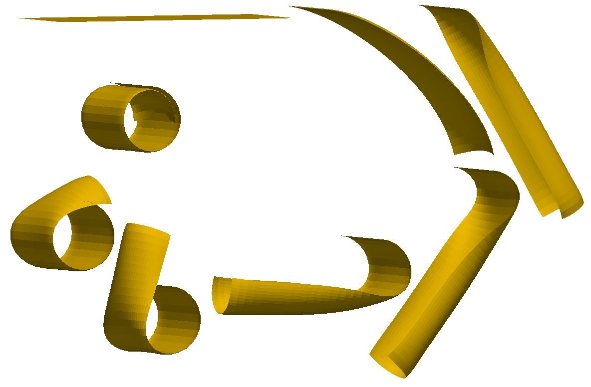
Figure 3. Pseudo-evolution (clockwise) towards the equilibrium of a clamped rectangular plate with spontaneous curvature $Z=-I_{2}$. The bilayer plate is depicted (clockwise) for 0.0, 0.1, 2.4, 60.0, 100.0, 130.0, 135.0, 207.3 times $10^{3}$ iterations of Algorithm 2. The bilayer plate reaches a cylindrical shape asymptotically (limit of discrete gradient flow). This is an absolute minimizer.

6.2. Relaxation Process

We consider the clamped plate $\omega$ described in Section 6.1 for different spontaneous curvatures $Z$ as well as different discretization parameters $h,\tau$. The subiterations stopping tolerance for Algorithm 3 is $\delta_{\text{stop}}=10^{-3}$. We examine the relaxation process towards equilibrium for two different spontaneous curvatures, namely $Z=-I_{2},\,-5I_{2}$. According to [20], the absolute energy minimizers are cylinders of height 4 (length of the clamped side) and of radius $1$ and $1/5$ (reciprocal of the eigenvalues of $Z$) with an energy of $20$ and $500$, respectively.

Table 1 documents the influence of meshsize $h$ and pseudo-timestep $\tau$ on the equilibrium shape and corresponding energy. The cases $Z=-I_{2}$ and $Z=-5I_{2}$ are strikingly different. For $Z=-I_{2}$ the equilibrium shape is a cylinder (absolute minimizer) provided $\tau\leq C_{0}h$ for a sufficiently small constant $C_{0}$; see Figure 4 (left for $\tau=0.0025$ and middle for $\tau=0.005$). For $Z=-5I_{2}$, and regardless of the size of $\tau$, the plate never reaches a cylinder but other equilibrium configurations (local minimizers) with much higher energy than $500$; see Figure 4 (right). A plausible explanation is that the relatively large spontaneous curvature in the direction of the clamped side favors bending in such a direction, thereby creating a geometric obstruction to reaching a cylindrical shape.

Table 1 also provides information about the threshold of $\tau$ needed for convergence of the sub-iterations of Algorithm 3. This value, being sensitive to $\|Z\|_{L^{\infty}(\omega)}$, is more stringent for $Z=-5I_{2}$. In fact, such iterations fail to converge for $\tau=0.02$ and $Z=-5I_{2}$, whereas for $Z=-I_{2}$ give rise to a local minimizer. This is consistent with Remark 4.3, which establishes the pessimistic thresholds $\tau_{0}=2.5\cdot 10^{-3}$ for $Z=-I_{2}$ and $\tau_{0}=10^{-4}$ for $Z=-5I_{2}$ if we consider a Poincaré constant $c_{P}=10$.

In addition, we note that the case $\tau=0.00125$ on the mesh #6 and with $Z=-I_{2}$ yields a cylindrical equilibrium shape with energy of $17.2$ (not reported in Table 1). This, in conjunction with the energies when $\tau=0.005$ on the mesh resulting from four refinements and $\tau=0.0025$ on the mesh resulting from five refinements, illustrates that $\widetilde{E}_{h}[{\bf y}_{h}^{\infty}]\to E[{\bf y}]=20$ as $h\to 0$, $h=c\tau$ and $c$ is sufficiently small to obtain cylindrical shapes. This is in accordance with Corollary 4.1.

	$Z=-I_{2}$				$Z=-5I_{2}$
	#4	#5	#6	#7	#4	#5	#6	#7
0.02	19.781n	20.351n	N/A	N/A	NoC	NoC	N/A	N/A
0.01	19.335n	20.157n	20.576n	19.590n	575.372	521.297	536.036	586.839
0.005	15.961y	16.554y	20.343n	N/A	567.886	519.599	534.365	N/A
0.0025	15.765y	16.395y	17.304y	18.062y	581.405	518.897	N/A	N/A

Table 1. Equilibrium energies $\widetilde{E}_{h}[{\bf y}_{h}^{\infty}]$ for spontaneous curvatures $Z=-I_{2},-5I_{2}$ and different meshsizes $h$ and pseudo-timesteps $\tau$. The meshes correspond to 4, 5, 6, and 7 uniform refinements of the plate $\omega=(-5,5)\times(-2,2)$. The symbol next to the energy values for $Z=-I_{2}$ indicates whether the equilibrium shape is a cylinder (y) or not (n) after the stopping test (6.1) is met. Typical equilibria are displayed in Figure 4 (left and middle, the latter corresponding to a local discrete minimizer). The numerical experiments indicate that the cylindrical shape (absolute minimizer) is reached for $Z=-I_{2}$ when $\tau$ and $h$ satisfy $\tau\leq C_{0}h$ for a sufficiently small constant $C_{0}$. This experimental condition is more restrictive than the theoretically derived condition for mere convergence of our numerical scheme. The symbol NoC for $Z=-5I_{2}$ indicates that the sub-iterations of Algorithm 3 did not converge. The cylindrical shape is never reached for $Z=-5I_{2}$; see Figure 4 (right) for a typical equilibrium configuration.

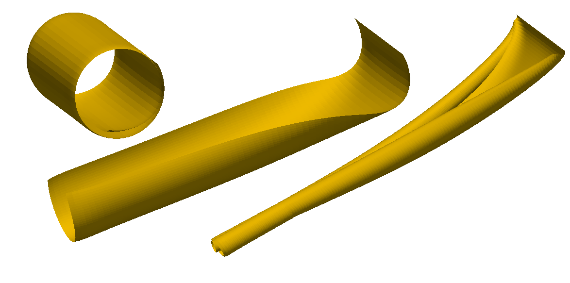
Figure 4. Equilibrium configurations of clamped rectangle plates $\omega=(-5,5)\times(-2,2)$ described in Section 6.1 for different spontaneous curvatures and numerical parameters. Left: cylinder shape when $Z=-I_{2}$, mesh refinement 6 and $\tau=0.0025$; Middle: local minimum when $Z=-I_{2}$, mesh refinement 6 and $\tau=0.005$; Right: local minimizer when $Z=-5I_{2}$, mesh refinement 7 and $\tau=0.01$. If the spontaneous curvature is $1$ or smaller, then the cylinder (absolute minimizer) is reached when the pseudo-timestep and the meshsize satisfy $\tau\leq C_{0}h$ for a sufficiently small constant $C_{0}$. For relatively large spontaneous curvatures, the curvature in the direction of the clamped side prevents the plate from bending completely in the orthogonal direction, thereby creating a geometric obstruction and leading to a (discrete) local minimizer for all numerical parameters tried.

6.3. Asymptotics

In this section, we illustrate the predicted convergence rate of $O(\tau)$ for the violation of the isometry constraint in (5.5). We consider again the clamped plate $\omega=(-5,5)\times(-2,2)$ described in Section 6.1 with a spontaneous curvature $Z=-I_{2}$. The space discretizations are subordinate to $4,5,6$ and $7$ uniform refinements of the initial partition of the plate consisting of 1 rectangle and are referred to as mesh $\#4,\#5,\#6$ and $\#7$, respectively. The sub-iterations stopping tolerance of Algorithm 3 is $\delta_{\text{stop}}=10^{-3}$. The equilibrium isometry defect is defined to be

$$ID_{h}({\bf y}_{h}^{\infty}):=\frac{\|[\nabla_{h}{\bf y}_{h}^{\infty}]^{\rotatebox[origin={c}]{180.0}{\footnotesize$\perp$}}[\nabla_{h}{\bf y}_{h}^{\infty}]-I_{2}\|_{L_{h}^{1}(\omega)}}{|\omega|}.$$

The results reported in Table 2 indicate that the predicted rate of convergence $O(\tau)$ in Proposition 5.2 is recovered numerically. This happens for both decreasing time steps $\tau$ on a fixed mesh (columns 1, 2, and 3) as well as simultaneous reduction of $h$ and $\tau$ while keeping $h\sim\tau$ (diagonal). We stress that, according to the discussion of Section 6.2, not all equilibrium configurations are cylinders but the experimentally observed linear rate applies to all of them. This is consistent with Proposition 5.2 which is not specific to absolute minimizers.

	#4	#5	#6	#7
0.02	0.0559	0.0488	N/A	N/A
0.01	0.0327	0.0283	0.0249	0.0276
0.005	0.0180	0.0155	0.0139	N/A
0.0025	0.0094	0.0081	0.0077	0.0083

Table 2. Isometry defect $ID_{h}({\bf y}_{h}^{\infty})$ for the clamped plate $\omega=(-5,5)\times(-2,2)$ at equilibrium with spontaneous curvature $Z=-I_{2}$. A sequence of time steps $\tau=0.02\times 2^{-i}$, $i=0,1,2,3$, is considered for different space resolutions. A decay rate $O(\tau)$ is observed when the space discretization remains unchanged (columns 1, 2 and 3) as well as when the meshsize is reduced to satisfy $h\sim\tau$ (diagonal). Notice that the isometry defect for a fixed time step is little affected by the space resolution (rows 2 and 4).

For an experimental convergence test for the deformations we choose $\omega=(0,2\pi)^{2}$, define

$$Z=-\left(\begin{array}[]{cc}1&0\\ 0&.5\end{array}\right),$$

and consider clamped boundary conditions on the left side $\partial_{D}\omega=\{x=0\}\times[0,2\pi]$. An exact solution is given by

$${\bf y}(x,y)=\big{(}\sin(x),y,1-\cos(x)\big{)}.$$

Table 3 shows the scaled $L^{2}$ and $H^{1}$ errors for the stationary configurations computed with Algorithms 2 and 3; norms were computed with a one-point Gaussian quadrature rule on every element. The stopping criterion for the fixed-point iteration is $\delta_{\rm stop}=10^{-4}$. The underlying meshes correspond to $\ell=3,4,5,6$ refinements of our coarse mesh so that $h_{\ell}=2\pi 2^{-\ell}$. We choose a step size proportional to the mesh size, i.e., we set $\tau_{\ell}=2^{-\ell}/25$ for $\ell=3,4,5,6$. The obtained errors indicate a nearly linear experimental convergence rate.

	#3	#4	#5	#6
$\|{\bf e}_{h}\|/|\omega|^{1/2}$	0.8250	0.4273	0.2310	0.1220
$\|\nabla{\bf e}_{h}\|/|\omega|^{1/2}$	0.6723	0.3622	0.2002	0.1077

Table 3. Scaled approximation errors ${\bf e}_{h}={\bf y}-{\bf y}_{h}^{\infty}$ in an experimental convergence test with exact solution ${\bf y}$ given by a cylinder of radius 1. The approximations ${\bf y}_{h}^{\infty}$ are obtained with Algorithms 2 and 3 from a flat initial configuration and timestep sizes proportional to meshsizes. The numbers indicate a nearly linear experimental convergence rate.

6.4. Effect of Aspect Ratio and Spontaneous Curvature

This section investigates numerically the influence of (i) the spontaneous curvature (i.e. difference in material properties between the two plates) and (ii) the plates aspect ratio. The numerical parameters in Algorithm 3 are $\tau=0.005$, $\delta_{\text{stop}}=10^{-4}$, and the partition corresponds to $5$ uniform refinements of the initial plate.

We consider plates $\omega:=(-L,L)\times(-2,2)$ with different lengths $L>0$ and define the aspect ratio to be $\rho:=L/2$. The plates are clamped on the side $\partial_{D}\omega=\{x=-L\}\times[-2,2]$. It turns out that the tendency to bend in the clamped direction (accentuated for relatively large spontaneous curvatures in the clamped direction according to Section 6.3) is attenuated for small aspect ratios. We illustrate this in Figure 5, which displays almost equilibrium configurations for $\rho=5/2,3/2,1,1/2$ and spontaneous curvatures $Z=-rI_{2}$ with $r=1,{\color[rgb]{0,0,0}3},5$. For large spontaneous curvatures, Algorithm 2 did not always reach geometric equilibrium before the stopping test (6.1) was met. In addition, some pseudo-evolutions lead to severe folding and exhibit self-intersections, in which case they are no longer representative from the physics standpoint.

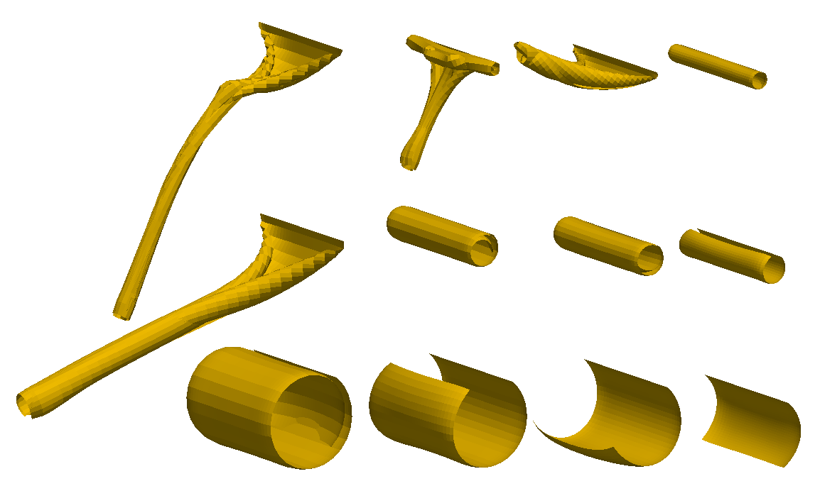
Figure 5. Equilibrium shapes of bilayer plates for several aspect-ratios $\rho$ (from left to right $\rho=5/2,3/2,1,1/2$) and spontaneous curvatures $Z=-rI_{2}$ (from top to bottom $r=5,3,1$). Decreasing the aspect ratio restores the ability for the plate to fold into a cylindrical shape for larger spontaneous curvatures. For instance, this is the case for plates with parameters $r=3$ and $\rho=3/2$ or $r=5$ and $\rho=1/2$. Notice, however, that small regions around the free corners have not completely relaxed to equilibrium. This effect is due to the violation of the isometry constraint and reduced upon decreasing the discretization parameters as well as the stopping criteria. The numbers below each stationary configuration are the corresponding approximate energies. For comparison, the energies of corresponding plates with principal curvatures of $\frac{1}{r}$ and $0$ are given between parenthesis.

6.5. Boundary Conditions and Shapes

We consider now different boundary conditions and plate shapes. We intend to examine the robustness of our numerical scheme in different situations and investigate plate shapes which are not studied in [20] and for which we do not know the absolute minimizers.

Boundary conditions: We start with the plate $\omega=(-3,3)\times(-2,2)$ clamped in a neighborhood of the bottom left corner, namely $\partial_{D}\omega=\{x=-3\}\times(-2,0)\cup(-3,0)\times\{y=-2\}$. We impose the spontaneous curvature $Z=-I_{2}$, choose the numerical parameters $\tau=0.005$, $\delta_{\text{stop}}=10^{-4}$ in Algorithm 3, and use a partition of $\omega$ with 5 uniform refinements. Several intermediate shapes of the discrete gradient flow are depicted in Figure 6. The equilibrium configuration consists of a flat and a cylindrical part separated by a free boundary that connects points on the boundary at which boundary conditions change.

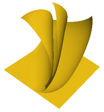
Figure 6. Different snapshots of the deformed corner-clamped plate with spontaneous curvature $Z=-I_{2}$. The equilibrium shape has energy $11.616$ and is not a cylinder. It is worth comparing with the side-clamped plate discussed in Section 6.4, which leads to a cylinder of smaller approximate energy $9.81$.

Shapes: We now consider the I-shaped and the O-shaped plates depicted in Figure 7. The finite element meshes contain $7168$ and $8192$ quasi-uniform rectangles respectively. We set $Z=-5I_{2}$, $\tau=0.005$ and $\delta_{\text{stop}}=10^{-3}$. Relaxation toward numerical equilibrium shapes, which are not cylinders, is depicted for both plates in Figure 8. We stress that for the I-shaped plate the curvature in the clamped direction dominates the other, thereby leading to a cigar shape that opens up at the bottom to accomodate the boundary condition. In contrast, the O-shaped plate is more rigid to bending and develops dog-ears at the free corners which prevent further bending.

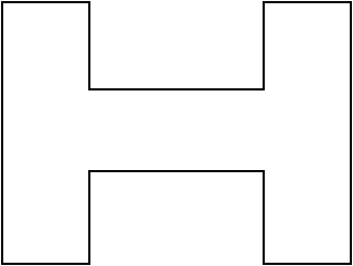
Figure 7. Geometry of the I-shaped and O-shaped plates: the numbers indicate the length of the sides. In both cases, the clamped edge is the far left vertical edge.

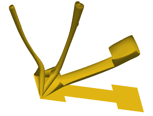
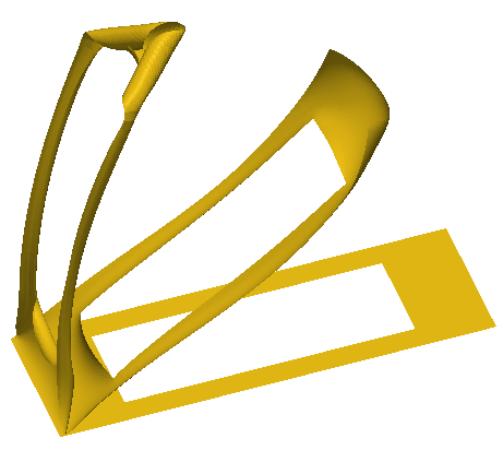
Figure 8. Different snapshots of the deformed I-shaped plate (left) and O-shaped plate (right). The corresponding stationary energies with spontaneous curvatures $Z=-5I_{2}$ are 404.57 and 314.152 respectively or about $12.448$ and $14.137$ relative to the plate areas. For comparison, the numerical stationary energy of a plate $\omega=(-5,5)\times(-2,2)$ under the same boundary condition and spontaneous curvature is $519.6$ or $12.99$ once divided by the plate area (see Figure 5). It turns out that compared to the full plate, the stationary numerical energy per unit area is smaller for the I-shaped plate and greater for the O-shaped plate.

6.6. Anisotropic Spontaneous Curvature

We now turn our attention to anisotropic spontaneous curvatures, namely to matrices $Z$ with different eigenvalues. In the first two examples the eigenvectors are aligned with the coordinate axis, but not in the third example. The spontaneous curvature is given by either

(6.2) $${Z=\left(\begin{array}[]{cc}-5&0\\ 0&-a\end{array}\right),\qquad Z=\left(\begin{array}[]{cc}-3&2\\ 2&-3\end{array}\right),}$$

with $a=1$ or $-5$. The plate is $\omega=(-2,2)\times(-3,3)$ and the numerical parameters in Algorithm 3 are $\tau=0.005,\delta_{\text{stop}}=10^{-3}$.

Dominant curvature: With $a=1$ being the curvature in the clamped direction, we notice a rather minimal bending effect in such a direction. The plate pseudo-evolutions are displayed in Figure 9 which shows an almost perfect rolling to a cylinder of energy $42.09$.

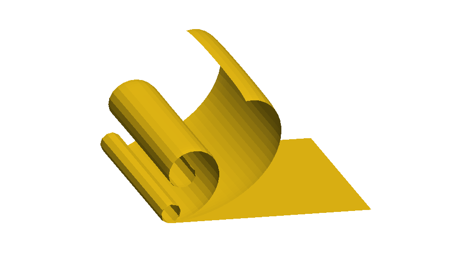
Figure 9. Deformation of a plate with anisotropic curvature given by (6.2) with $a=1$. The spontaneous curvature is $1$ in the clamped direction, its effect being barely noticeable, whereas it is $5$ in the orthogonal direction. The equilibrium shape is a cylinder (absolute minimizer) with an energy of $42.09$. Compare with the case $a=5$, presented in Section 6.4, for which the cylindrical shape is not achieved before the stopping test (6.1) is met.

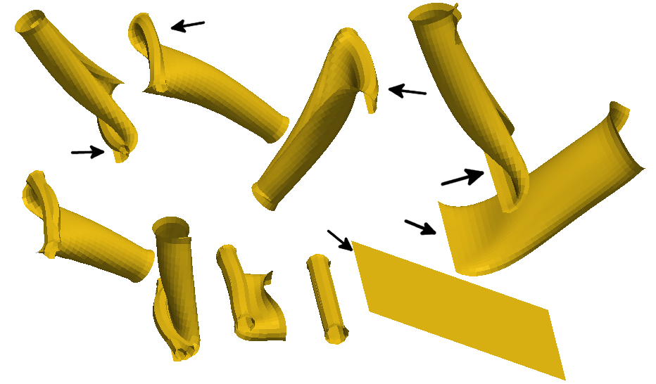
Figure 10. Deformation of a plate with anisotropic curvature given by (6.2) with $a=-5$. The spontaneous curvatures are $-5$ in the clamped direction and $5$ in the perpendicular direction, which eventually dominates the former and leads to a cylindical shape after three full rotations. Snapshots are displayed counterclockwise, starting from the bottom right, for 0.0, 0.3, 2.0, 4.0, 6.0, 10.0, 15.0, 18.0, 25.0, 172.0 times $10^{3}$ iterations of Algorithm 2. The arrows indicate the clamped side.

Curvatures with opposite signs: We take $a=-5$ to be the curvature in the clamped direction. This choice models the tendency of the plate to bend equally in opposite directions along the coordinate axes (principal directions). This is noticeable in the second and third snapshots in Figure 10, the latter also exhibiting self-crossing of the free corners. After three complete rotations, the plate relaxes to a cylindrical shape (absolute minimizer). Surprisingly, a cylindrical shape is reached before the stopping test (6.1) is met, unlike the case $a=5$ (see first row - second column in Figure 5).

Corkscrew shape: We consider now the second anisotropic spontaneous curvature $Z$ in (6.2), which has eigenpairs

$$\mu_{1}=5\quad{\bf e}_{1}=[1,-1]^{T},\qquad\mu_{2}=1\quad{\bf e}_{2}=[1,1]^{T}.$$

This means that we still have principal curvatures $5$ and $1$ but with principal directions ${\bf e}_{1}$ and ${\bf e}_{2}$ forming the angle $\pi/4$ with the coordinate axes. The deformation of this plate towards its equilibrium shape is displayed in Figure 11. The plate exhibits a corkscrew shape before self-intersecting and continuing its deformation to a conic shape. In fact, a cylindrical shape is not reached before the stationarity test (6.1) is met. We emphasize that this is not in contradiction with [20], where scalar spontaneous curvatures are considered, and shed some light on equilibrium configurations when the two principal spontaneous curvature directions are not parallel and orthogonal to the clamped side. Notice, however, that the equilibrium energy obtained is $61.31$, which is larger than the cylindrical shape obtained when the principal direction aligned with the coordinate axes (see Figure 9).

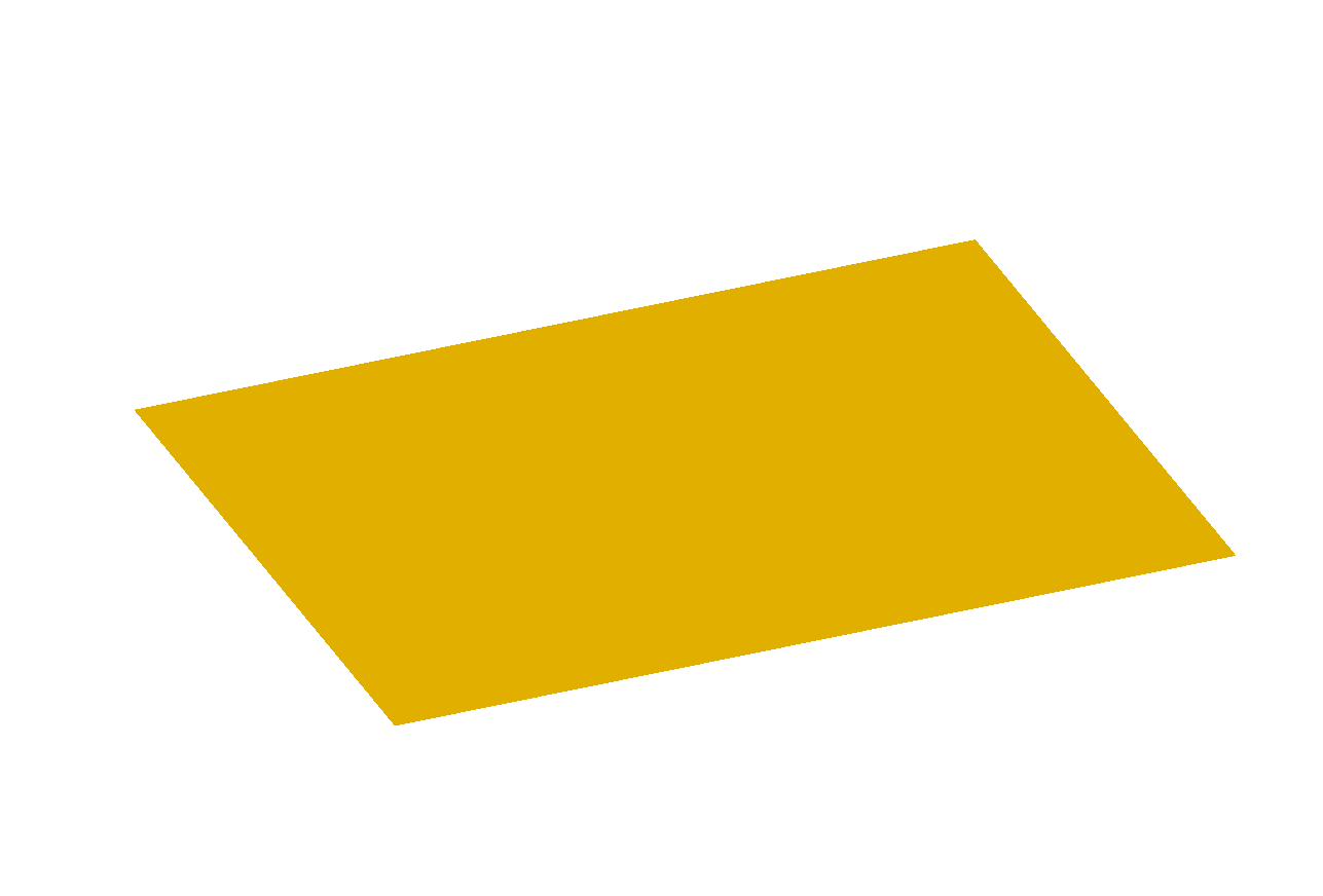
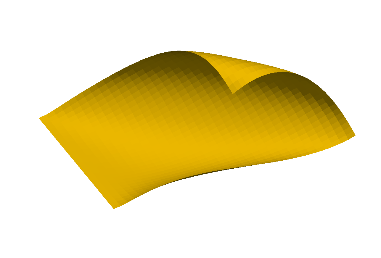
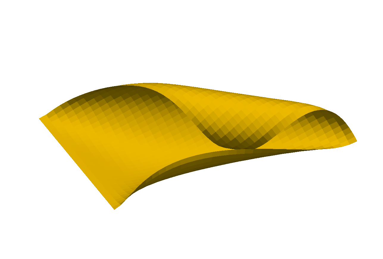
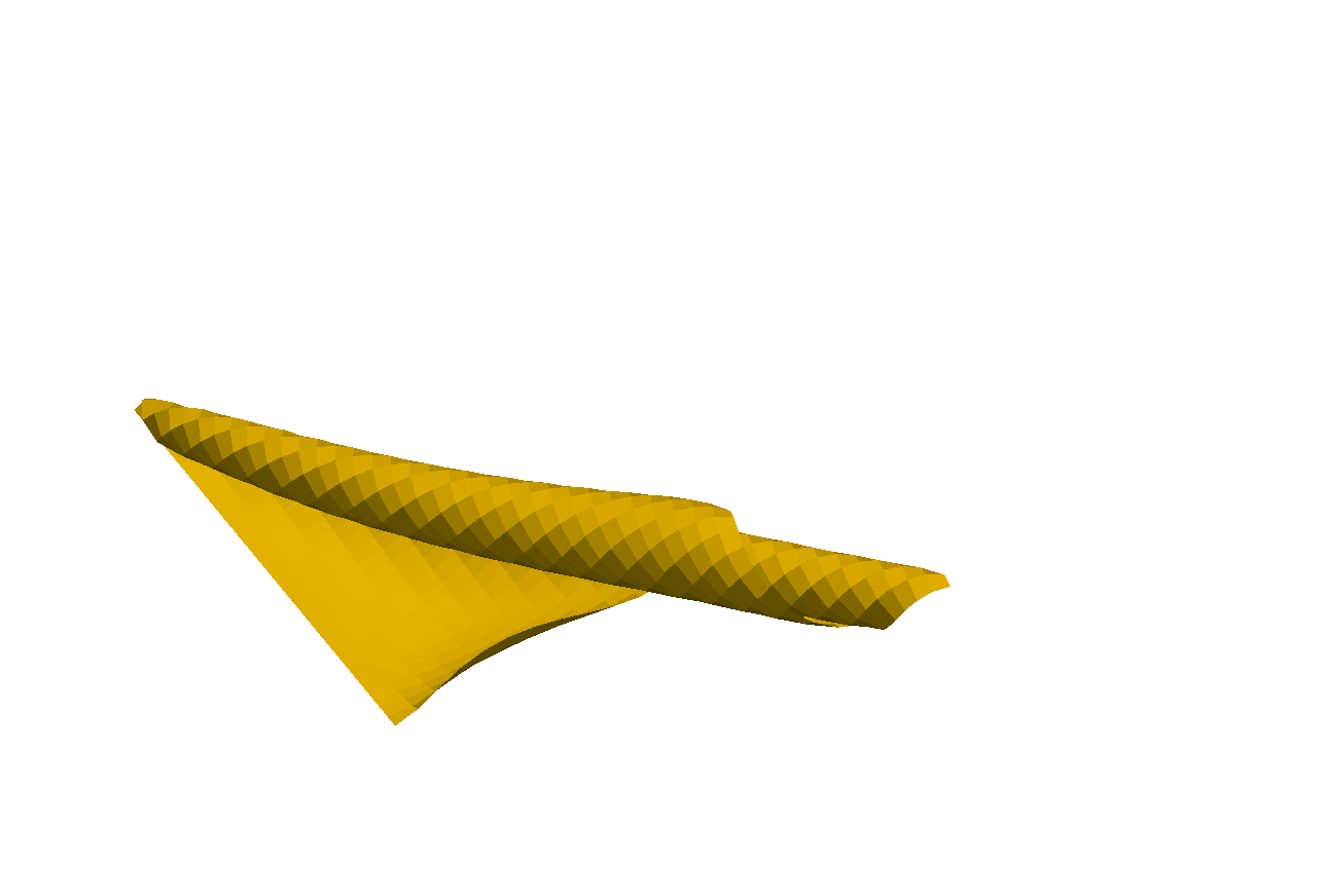
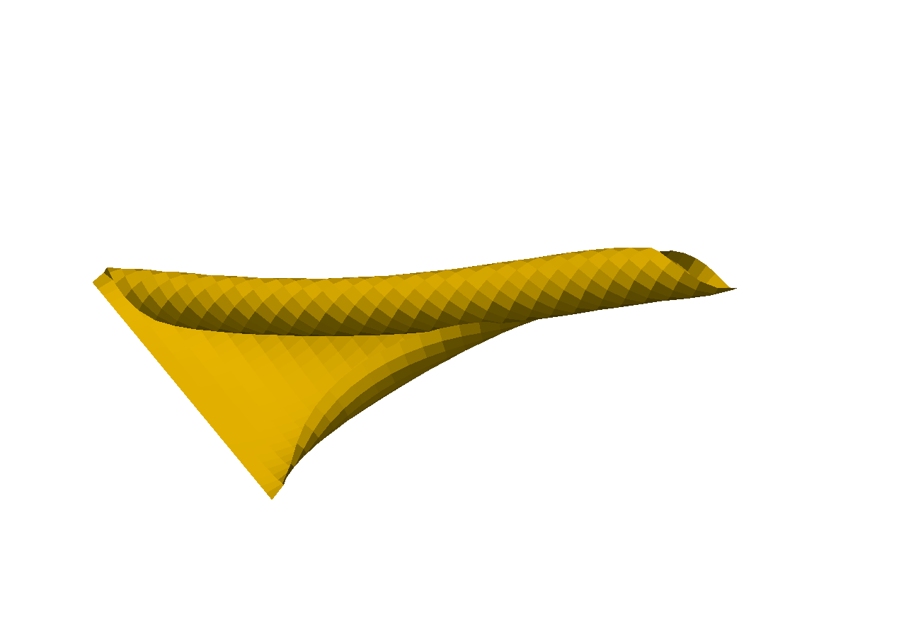
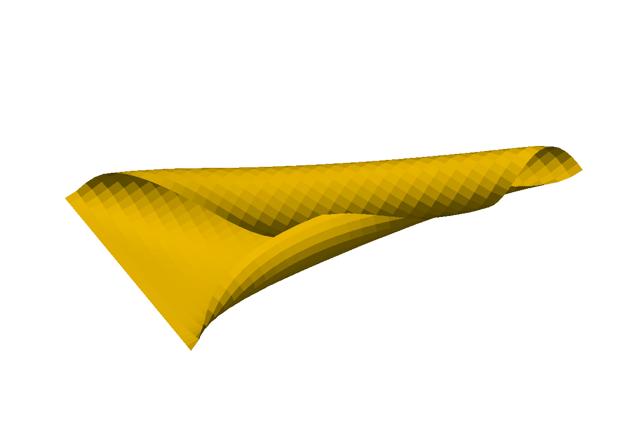
Figure 11. Deformation of a plate with the second anisotropic curvature $Z$ in (6.2). The principal curvatures are $5$ and $1$ but the principal directions form an angle $\pi/4$ with the coordinate axes. The snapshots are displayed clockwise starting at the top left, for 0.0, 0.1, 0.4, 1.9, 3.0, 324.0 times $10^{3}$ iterations of Algorithm 2. The plate adopts a corkscrew shape before self-intersecting.

6.7. Energy Decay and Time Scales

One critical aspect missing in this study is the design of (pseudo)-time adaptive algorithms able to cope with the disparate time scales inherent to the underlying energies. To illustrate this point, we plot in Figure 12 the energy decay of the clamped plate $\omega$ of Section 6.1 for spontaneous curvatures $Z=-I_{2}$ and $Z=-5I_{2}$. Both energies exhibit a rapid decay at the very beginning of the deformation and very slow decay at the end. The numerical parameters of Algorithm 3 used for these simulations are $\tau=0.005$, $\delta_{\text{stop}}=10^{-4}$ and the finite element partition corresponds to 5 uniform refinements of the original plate.

Figure 12. Energy decay versus pseudo-time for $Z=-rI_{2}$ with $r=1$ and $r=5$. The cylindrical shape is reached when $r=1$ after 207,000 pseudo-timesteps (total of 210.469 solves accounting for the sub iterations). When $r=5$, the equilibrium shape is reached faster after 86.600 pseudo-timesteps (total of 129.682 solves accounting for the sub iterations). However, the equilibrium reached is not a cylinder as already pointed out in Sections 6.2 and 6.4; see for instance Figure 4. The energy decays fast at the very beginning of the relaxation process in both cases. In addition when $r=1$, a second rapid decay arises with the unfolding in the clamped direction; see iteration 130,000 in Figure 3 (6th snapshot).

Acknowledgements. We are indebted to S. Conti who suggested a reduced model leading to that of Section 2. We are also thankful to E. Smela who stimulated our curiosity to study folding patterns of bilayer plates via several laboratory experiments and discussions. Finally, we express our gratitude to W. Bangerth for participating in several discussions regarding the implementation of the Kirchhoff quadrilaterals with deal.II [2].

References

[1]Alben, S., Balakrisnan, B., and Smela, E.Edge effects determine the direction of bilayer bending.
Nano Letters 11, 6 (2011), 2280–2285.
PMID: 21528897.
[2]Bangerth, W., Hartmann, R., and Kanschat, G.deal.II—a general-purpose object-oriented finite element library.
ACM Trans. Math. Software 33, 4 (2007), Art. 24, 27.
[3]Bartels, S.Approximation of large bending isometries with discrete Kirchhoff
triangles.
SIAM J. Numer. Anal. 51, 1 (2013), 516–525.
[4]Bartels, S.Numerical methods for nonlinear partial differential equations,
vol. 47 of Springer Series in Computational Mathematics.
Springer, 2015.
[5]Bassik, N., Abebe, B., Laflin, K., and Gracias, D.Photolithographically patterned smart hydrogel based bilayer
actuators.
Polymer 51 (2010), 6093???6098.
[6]Batoz, J.-L., Bathe, K.-J., and Ho, L.-W.A study of three-node triangular plate bending elements.
International Journal for Numerical Methods in Engineering 15,
12 (1980), 1771–1812.
[7]Batoz, J.-L., and Tahar, M. B.Evaluation of a new quadrilateral thin plate bending element.
International Journal for Numerical Methods in Engineering 18,
11 (1982), 1655–1677.
[8]Braess, D.Finite elements, third ed.
Cambridge University Press, Cambridge, 2007.
Theory, fast solvers, and applications in elasticity theory,
Translated from the German by Larry L. Schumaker.
[9]Braides, A.Local minimization, variational evolution and
-convergence, vol. 2094 of Lecture Notes in Mathematics.
Springer, 2014.
[10]Brenner, S. C., and Scott, L. R.The mathematical theory of finite element methods, third ed.,
vol. 15 of Texts in Applied Mathematics.
Springer, New York, 2008.
[11]Ciarlet, P. G.Mathematical elasticity. Vol. II, vol. 27 of Studies
in Mathematics and its Applications.
North-Holland Publishing Co., Amsterdam, 1997.
Theory of plates.
[12]Dal Maso, G.An introduction to -convergence.
Progress in Nonlinear Differential Equations and their Applications,
8. Birkhäuser Boston, Inc., Boston, MA, 1993.
[13]Davis, T. A.UMFPACK Version 5.2 Quick Start Guide, 2007.
[14]Friesecke, G., James, R. D., and Müller, S.A theorem on geometric rigidity and the derivation of nonlinear plate
theory from three-dimensional elasticity.
Comm. Pure Appl. Math. 55, 11 (2002), 1461–1506.
[15]Friesecke, G., James, R. D., and Müller, S.A hierarchy of plate models derived from nonlinear elasticity by
-convergence.
Arch. Ration. Mech. Anal. 180, 2 (2006), 183–236.
[16]Henderson, A., Ahrens, J., and Law, C.The ParaView Guide, kitware inc. ed., 2004.
[17]Hornung, P.Approximation of flat isometric immersions by smooth
ones.
Arch. Ration. Mech. Anal. 199, 3 (2011), 1015–1067.
[18]Jager, E., Smela, E., and Inganäs, O.Microfabricating conjugated polymer actuators.
Science 290 (2000), 1540???1545.
[19]Kuo, J.-N., Lee, G.-B., Pan, W.-F., and Lee, H.-L.Shape and thermal effects of metal films on stress-induced bending of
micromachined bilayer cantilever.
Japanese Journal of Applied Physics 44, 5R (2005), 3180.
[20]Schmidt, B.Minimal energy configurations of strained multi-layers.
Calc. Var. Partial Differential Equations 30, 4 (2007),
477–497.
[21]Schmidt, B.Plate theory for stressed heterogeneous multilayers of finite bending
energy.
J. Math. Pures Appl. (9) 88, 1 (2007), 107–122.
[22]Schmidt, O., and Eberl, K.Thin solid films roll up into nanotubes.
Nature 410 (2001), 168.
[23]Smela, E., Inganös, O., and Lundström, I.Controlled folding of micrometer-size structures.
Science 268, 5218 (1995), 1735–1738.
[24]Smela, E., Inganös, O., Pei, Q., and Lundström, I.Electrochemical muscles: Micromachining fingers and corkscrews.
Advanced Materials 5, 9 (1993), 630–632.