Quantum theory as a description of robust experiments: Application to Stern-Gerlach and Einstein-Podolsky-Rosen-Bohm experiments

Abstract

We propose and develop the thesis that the quantum theoretical description of experiments emerges from the desire to organize experimental data such that the description of the system under scrutiny and the one used to acquire the data are separated as much as possible. Application to the Stern-Gerlach and Einstein-Podolsky-Rosen-Bohm experiments are shown to support this thesis. General principles of logical inference which have been shown to lead to the Schrödinger and Pauli equation and the probabilistic descriptions of the Stern-Gerlach and Einstein-Podolsky-Rosen-Bohm experiments, are used to demonstrate that the condition for the separation procedure to yield the quantum theoretical description is intimately related to the assumptions that the observed events are independent and that the data generated by these experiments is robust with respect to small changes of the conditions under which the experiment is carried out.

1 Introduction

As quantum theory has proven remarkably powerful to describe many very different experiments in (sub)-atomic, molecular and condensed matter physics, quantum optics and so on, it is of interest to search for explanations that go beyond “that is because of the way it is”. Recently, several papers [1, 2, 3] suggest that such an explanation can be given. Some of the most basic elements of quantum theory, such as the Schrödinger equation, have been derived [1, 2, 3] by taking the mathematical framework of logical inference (LI) [4, 5, 6, 7, 8] as a basis for establishing a bridge between the data gathered through experiments and their description in terms of (mathematical) concepts. These papers are not concerned with the various interpretations of quantum theory [9, 10, 11, 12] but employ a mathematically precise formalism that expresses what most people would consider to be rational reasoning. The key concept is the notion of the plausibility that a proposition is true [4, 5, 6, 7, 8].

The basic premise of the LI approach [1, 2, 3] is that scientific theories are created through cognitive processes in the human brain, based on discrete events which are observed in every-day life and in laboratory experiments combined with the logical and/or cause-and-effect relations between those events that we, humans, uncover. Because of this premise, the LI approach does not depend on assumptions such as that the observed events are signatures of an underlying objective reality – which may or may not be mathematical in nature, that all things physical are information-theoretic in origin, that the universe is participatory etc.

The rules of LI are not bound by “laws of physics”. LI applies to situations where there may or may not be causal relations between the events [6, 8]. Although extracting cause-and-effect relationships from empirical evidence is a highly non-trivial problem, rational reasoning about these relations should comply with the rules of LI. However, in general, the latter cannot be used to establish cause-and-effect relationships themselves [8, 13, 14]. A derivation of a quantum theoretical description from LI principles does not prohibit the construction of cause-and-effect mechanisms that create the impression that these mechanisms produce data that can be described by quantum theory [15]. In fact, there is a substantial body of work demonstrating that it is indeed possible to build simulation models which reproduce, on an event-by-event basis, the results of interference/entanglement/uncertainty experiments with single photons/neutrons [16, 17, 18, 19, 20].

In the LI approach it is not necessary to assume that the observed events are “generated” according to some (quantum) laws. These laws naturally emerge from inference based on available data. There is no need to postulate “wavefunctions”, “wavefunction collapse”, “observables”, “quantization rules”, “Born’s rule”, “wave-particle duality” etc. and there is no “quantum measurement problem” [21]. For a particle in a (electromagnetic) potential, the solution of the inference problem takes the form of a set of non-linear equations and the Schrödinger and Pauli equation appear as a result of transforming this set into a set of linear equations which are much more convenient for further analysis [1, 2, 3].

The mathematical framework of LI [4, 5, 6, 7, 8] applied to basic problems such as the idealized Stern-Gerlach (SG) and Einstein-Podolsky-Rosen-Bohm (EPRB) experiments also yield the probability distributions that we know from quantum physics [2]. However, unlike in the case of the particle in a potential where the Schrödinger and Pauli equation appear as a result of transforming a set of non-linear equations into a set of linear equations, for the SG and EPRB experiment Ref. [2] did not explicitly derive the wavefunction (density matrix) description but was content by showing that the robust solution of the inference problem yields the expressions of the probabilities that are known from quantum theory [2]. In this paper, we fill this void by demonstrating, using the SG and EPRB experiment as concrete examples, how the mathematical structure of quantum theory naturally emerges from the desire to organize experimental data such that it separates as much as possible, the description of the system under scrutiny from the description of the probe used to acquire the data.

The idea that the mathematical structure of quantum theory has application to cognitive science, psychology, genetics, economics, finances, and game theory is discussed in great depth by Khrennikov [22]. Building on the “wavefunction postulate”, Khrennikov shows how to construct contextual probabilistic models of natural, biological, psychological, social, economical or financial phenomena [22]. In particular, Born’s rule appears by representing probabilistic data in terms of complex probability amplitudes [22]. The route taken in the present paper is complementary and more along the line of thinking explored in Ref. [23].

A general, characteristic feature of scientific reasoning is that it strives to reduce the complexity of the description of the whole by separating the description of data into several independent parts. The separation of variables when solving differential equations, the Fourier analysis of a signal, a principal component analysis of a correlation matrix of data, the normal mode description of the vibrations in a harmonic solid, are just a few of the vast set of instances where this division is used to great advantage. In the present paper, we start by considering different ways of organizing observed data and scrutinize the conditions for which the data can be represented such that the description of the various components of the experimental setup can be separated as much as possible. We show that the wavefunction description appears as the result of such a separation procedure. It automatically follows that the wavefunction (or density matrix) description is less general than the one in terms of conditional probabilities in the sense that the former can only describe situations in which the separation procedure can actually be carried out.

The paper is structured as follows. Section 2 starts with the analysis of data produced by an idealized SG experiment. We show how compression of data and subsequent reorganization offers the possibility to separate the description of the source and the magnet in this particular case, leading to the quantum theoretical description in terms of a wavefunction of a spin-1/2 system. Then, we briefly recapitulate how the LI approach directly leads to the probabilities for observing the events and show how the results of quantum theory emerge without invoking any of its postulates. In Section 3, we apply the same logic to the EPRB thought experiment and demonstrate how the singlet state emerges by rearranging the data such that separation becomes possible. Although this derivation does not add anything new to the ongoing discussions about locality, realism, etc. in relation to the violation of Bell-like inequalities [24, 25, 26, 27, 28, 29, 30, 31, 32, 33, 34, 35, 36, 37, 38], it does de-mystify the “origin” and “nature” of quantum entanglement.

2 Idealized Stern-Gerlach experiment

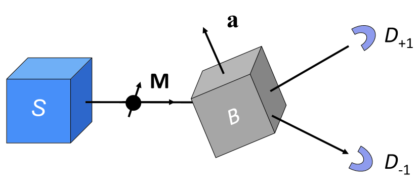
Figure 1: (Color online) Diagram of the SG experiment. The source $S$, activated at times labeled by $i=1,2,\ldots,N$, sends a particle carrying a magnetic moment $\mathbf{M}$ to the magnet $B$ with its (inhomogeneous) magnetic field along the direction $\mathbf{a}$. Depending on the relative directions of $\mathbf{a}$ and $\mathbf{M}$, the particle is detected with 100% certainty by either $D_{+1}$ or $D_{-1}$.

In the idealized SG experiment, a schematic of which is shown in Fig. 1, there are two different outcomes which we label by the variable $x$ taking the values $+1$ or $-1$. We imagine that the experiment is repeated $N$ times, yielding the data set

$${\cal D} = \big{\{}x_{1},\ldots,x_{N}|x_{i}=\pm 1\;,i=1,\ldots,N\big{\}}.$$ (1)

Assuming that the observed $x_{i}$ are independent events (uncorrelated in time), the data is completely characterized by the counts $N(+1|\mathbf{a},\mathbf{M},Z)$ of outcomes with $x=+1$ and $N(-1|\mathbf{a},\mathbf{M},Z)$ of outcomes with $x=-1$ where $N=N(+1|\mathbf{a},\mathbf{M},Z)+N(-1|\mathbf{a},\mathbf{M},Z)$. Here and in the following, we use the notation “$|a,b,\ldots)$” to indicate that the data is collected under the ${\it fixed}$ conditions $a,b,\ldots$. In the case at hand, $\mathbf{a}$, $\mathbf{M}$, and $Z$ represent, respectively, a unit vector specifying the direction of the SG magnet, a unit vector representing the direction of the magnetic moments of the incoming particles, and all other fixed conditions which are important to the actual experiment but are not of immediate interest. Assuming independent $x_{i}$’s, the average reads

$$\langle x\rangle = \sum_{x=\pm 1}xf(x|\mathbf{a},\mathbf{M},Z)\quad,\quad f(x|\mathbf{a},\mathbf{M},Z)\equiv N(x|\mathbf{a},\mathbf{M},Z)/N,$$ (2)

where $f(x|\mathbf{a},\mathbf{M},Z)$ denotes the (empirical) frequency of observing the event $x$ and completely characterizes the outcomes of an idealized SG experiment of $N$ events. As $f(x|\mathbf{a},\mathbf{M},Z)$ is a function of the two-valued variable $x$, it can be written as

$$f(x|\mathbf{a},\mathbf{M},Z) = \frac{1+xE(\mathbf{a},\mathbf{M},Z)}{2},$$ (3)

where $E(\mathbf{a},\mathbf{M},Z)=\langle x\rangle$. Assuming that the observed counts do not depend on the orientation of the chosen reference frame, $E(\mathbf{a},\mathbf{M},Z)$ can only depend on $\mathbf{a}\cdot\mathbf{M}$ (by construction $|\mathbf{a}|=1$ and $|\mathbf{M}|=1$). Hence, we must have $f(x|\mathbf{a},\mathbf{M},Z)=f(x|\mathbf{a}\cdot\mathbf{M},Z)$.

2.1 Separation procedure

It is obvious from Eq. (2) that the description in terms of $x$ and $f(x|\mathbf{a},\mathbf{M},Z)$ does not readily allow for the separation that we envisage. Therefore, it is necessary to consider rewritings of Eq. (2) that lend themselves to such a separation.

Let us organize data of observations and frequencies in vectors $\mathbf{x}=(+1,-1)^{T}$ and $\mathbf{f}=(f(+1|\mathbf{a},\mathbf{M},Z),f(-1|\mathbf{a},\mathbf{M},Z))^{T}$, respectively. Then, we have

$$\langle x\rangle = \mathbf{x}^{T}\cdot\mathbf{f}=\mathbf{Tr\;}\mathbf{x}^{T}\mathbf{f}=\mathbf{Tr\;}\mathbf{f}\mathbf{x}^{T},$$ (4)

where $\mathbf{f}\mathbf{x}^{T}$ is a $2\times 2$ matrix and $\mathbf{Tr}\;A$ denotes the trace of the matrix $A$.

The key to the separation procedure is to note that any rewriting of $\mathbf{x}$ and $\mathbf{f}$ in terms of vectors, matrices, …, $\widetilde{\mathbf{x}}$ and $\widetilde{\mathbf{f}}$ such that $\mathbf{Tr\;}\widetilde{\mathbf{f}}=1$ and $\mathbf{Tr\;}\widetilde{\mathbf{f}}\widetilde{\mathbf{x}}=\langle x\rangle$ hold may be useful. With this in mind, we consider the rearrangement of the data into $2\times 2$ (diagonal, hermitian) matrices $X$ and $F$ with elements $X(x,x^{\prime})=x\delta_{x,x^{\prime}}$ and $F(x,x^{\prime})=f(x|\mathbf{a},\mathbf{M},Z)\delta_{x,x^{\prime}}$, respectively. Then, Eq. (4) can be written as

$$\langle x\rangle = \mathbf{Tr}\;FX=\mathbf{Tr}\;\widehat{\rho}\widehat{X},$$ (5)

where $\widehat{\rho}$ and $\widehat{X}$ can be any pair of $2\times 2$ matrices that satisfies Eq. (5). As Eq. (5) is just a formal rewriting of Eq. (4) it can, by itself, not bring anything new. Clearly, in the original representation of the data Eq. (2), separation is impossible (as it is implicitly assumed that $f(x|\mathbf{a},\mathbf{M},Z)$ does indeed depend on $\mathbf{a}$, $\mathbf{M}$, and $Z$). However, the flexibility offered by representation Eq. (5) allows us to perform the separation, as we now show.

From linear algebra, we know that any hermitian $2\times 2$ matrix can be written as a linear combination of four hermitian $2\times 2$ matrices. These four matrices may be chosen such that they are orthonormal with respect to the inner product defined by $(A,B)=\mathbf{Tr}\;A^{\dagger}B$. Using the Pauli-spin matrices $\bm{\sigma}=(\sigma^{x},\sigma^{y},\sigma^{z})$ and the unit matrix 11 as the orthonormal basis set for the vector space of $2\times 2$ matrices, we may write (without loss of generality)

$$\widehat{\rho}=\frac{\rho_{0}\leavevmode\hbox{\small 1\normalsize\kern-3.30002pt1}+\bm{\rho}\cdot\bm{\sigma}}{2}\quad,\quad\widehat{X}=u_{0}\leavevmode\hbox{\small 1\normalsize\kern-3.30002pt1}+\mathbf{u}\cdot\bm{\sigma}.$$ (6)

where $\rho_{0}$, $\bm{\rho}=(\rho_{x},\rho_{y},\rho_{z})$, $u_{0}$, and $\mathbf{u}=(u_{x},u_{y},u_{z})$ are real-valued objects. Using $(\mathbf{a}\cdot\bm{\sigma})\;(\mathbf{b}\cdot\bm{\sigma})=\mathbf{a}\cdot\mathbf{b}+i(\mathbf{a}\times\mathbf{b})\cdot\bm{\sigma}$ we find

$$2\widehat{\rho}\widehat{X}=u_{0}\rho_{0}\leavevmode\hbox{\small 1\normalsize\kern-3.30002pt1}+u_{0}\bm{\rho}\cdot\bm{\sigma}+\rho_{0}\mathbf{u}\cdot\bm{\sigma}+\bm{\rho}\cdot\mathbf{u}\leavevmode\hbox{\small 1\normalsize\kern-3.30002pt1}+i(\bm{\rho}\times\mathbf{u})\cdot\bm{\sigma}.$$ (7)

Making use of $\mathbf{Tr}\;\leavevmode\hbox{\small 1\normalsize\kern-3.30002pt1}=2$ and $\mathbf{Tr}\;\bm{\sigma}=0$ we find

$$\mathbf{Tr}\;\widehat{\rho}=\rho_{0}\quad,\quad\mathbf{Tr}\;\widehat{\rho}\widehat{X}=\rho_{0}u_{0}+\bm{\rho}\cdot\mathbf{u}.$$ (8)

Note that unlike $FX$, the matrix Eq. (7) is not hermitian. Obviously, useful alternative representations of the data should not change the description of the data, that is we should impose the constraints $\mathbf{Tr}\;F=\mathbf{Tr}\;\widehat{\rho}=1$ and $\mathbf{Tr}\;FX=\mathbf{Tr}\;\widehat{\rho}\widehat{X}$. Hence, from Eqs. (5) and (8) it follows that

$$\langle x\rangle = u_{0}+\bm{\rho}\cdot\mathbf{u},$$ (9)

suggesting that the desired separation can be realized by requiring that $u_{0}=u_{0}(\mathbf{a},Z)$, $u_{x}=u_{x}(\mathbf{a},Z)$, $u_{y}=u_{y}(\mathbf{a},Z)$, $u_{z}=u_{z}(\mathbf{a},Z)$, $\rho_{x}=\rho_{x}(\mathbf{M},Z)$, $\rho_{y}=\rho_{y}(\mathbf{M},Z)$, and $\rho_{z}=\rho_{z}(\mathbf{M},Z)$ (recall that $Z$ is considered to represent all fixed conditions which are important to the actual experiment but are not of immediate interest). Assuming that the observed counts do not depend on the orientation of the reference frame (see earlier), $\langle x\rangle$ is a function of $\mathbf{a}\cdot\mathbf{M}$ only. This requirement enforces $\bm{\rho}=\mathbf{M}$, and $\mathbf{u}=\mathbf{a}$. Hence, we have

$$\langle x\rangle = u_{0}+\mathbf{M}\cdot\mathbf{a}.$$ (10)

As $|\langle x\rangle|\leq 1$ it follows from Eq. (10) that $-1\leq u_{0}+\mathbf{M}\cdot\mathbf{a}\leq 1$. As the unit vector $\mathbf{a}$ can take any value on the unit sphere, we find that $u_{0}\leq 0$ and $0\geq u_{0}$ for $\mathbf{a}=\mathbf{M}$ and $\mathbf{a}=-\mathbf{M}$, respectively, hence $u_{0}=0$. Note that we have tactically written $\bm{\rho}=\mathbf{M}$, and $\mathbf{u}=\mathbf{a}$ but it is clear that at this point, we could equally well have made the choice $\bm{\rho}=\mathbf{a}$, and $\mathbf{u}=\mathbf{M}$. However, the latter choice leads to inconsistencies when we consider for instance an experiment in which we place several SG magnets in succession or consider the EPRB experiment (see Section 3).

We may therefore conclude that the desire to represent the data Eq. (1) such that the description of the whole experiment is separated into a description of the “source” ($\mathbf{M}$) and a description of the “measurement device” ($\mathbf{a}$) leads to the unique representation in terms of $2\times 2$ matrices

$$\widehat{\rho}=(\leavevmode\hbox{\small 1\normalsize\kern-3.30002pt1}+\mathbf{M}\cdot\bm{\sigma})/2\quad,\quad\widehat{X}=\mathbf{a}\cdot\bm{\sigma},$$ (11)

conditional on the assumptions that the individual outcomes of a SG experiment are independent and that the frequency distribution of these outcomes does not depend on the orientation of the reference frame.

From Eq. (11) it follows immediately that $\widehat{\rho}^{2}=\widehat{\rho}$, that is $\widehat{\rho}$ is a projection. This implies that we can write [39]

$$\widehat{\rho}=|\Psi\rangle\langle\Psi|\quad,\quad|\Psi\rangle=a_{\uparrow}|\uparrow\rangle+a_{\downarrow}|\downarrow\rangle.$$ (12)

where the vector $|\Psi\rangle$ is expressed in the basis of the eigenstates ($|\uparrow\rangle$,$|\downarrow\rangle$) of the $\sigma^{z}$ matrix. Therefore, we may conclude that in the case of the SG experiment, changing the representation of the data in combination with the desire to separate as much as possible the description of the source and measurement devices automatically enforces the Hilbert space structure that is a characteristic signature of quantum theory.

Starting from Eq. (11) we can construct a mixed state [39] by multiplying Eq. (11) with $w(\mathbf{M})d\mathbf{M}$ and integrating over $\mathbf{M}$, $w(\mathbf{M})$ being the probability density of $\mathbf{M}$. This changes Eq. (11) into

$$\widehat{\rho}=(\leavevmode\hbox{\small 1\normalsize\kern-3.30002pt1}+\langle\mathbf{M}\rangle\cdot\bm{\sigma})/2\quad,\quad\widehat{X}=\mathbf{a}\cdot\bm{\sigma},$$ (13)

where $\langle\mathbf{M}\rangle=\int\mathbf{M}\;w(\mathbf{M})d\mathbf{M}$. Then $\widehat{\rho}^{2}\not=\widehat{\rho}$ if $|\langle\mathbf{M}\rangle|<1$. Therefore, under the conditions stated, the separation procedure yields the more general mixed-state description of a spin-1/2 object. Applying the same reasoning to generalize the “unseparated” description, we have

$$\langle x\rangle=\int\frac{1+xE(\mathbf{a}\cdot\mathbf{M},Z)}{2}w(\mathbf{M})d\mathbf{M}=\frac{1+x\langle E(\mathbf{a}\cdot\mathbf{M},Z)\rangle}{2},$$ (14)

where $\langle E(\mathbf{a}\cdot\mathbf{M},Z)\rangle=\int E(\mathbf{a}\cdot\mathbf{M},Z)w(\mathbf{M})d\mathbf{M}$. In general, $\langle E(\mathbf{a}\cdot\langle\mathbf{M}\rangle,Z)\rangle\not=E(\mathbf{a}\cdot\langle\mathbf{M}\rangle,Z)$. Hence, even before we attempt to separate the descriptions, it is clear that Eq. (14) can describe experimental data that cannot be represented by Eq. (13). Moreover, there is nothing that forbids an experiment to yield for instance $E(\mathbf{a}\cdot\langle\mathbf{M}\rangle),Z)=(\mathbf{a}\cdot\langle\mathbf{M}\rangle)^{2}$ (we certainly can generate such data using a digital computer, a physical device on which we carry out experiments) but the data produced by such an experiment cannot be represented by Eq. (11). In other words, the class of conceivable SG experiments is significantly larger than the class of experiments that allows for the separation, that is this class is (much) larger than the class of SG experiments describable by quantum theory.

Summarizing: we have derived the quantum theoretical description of the idealized SG experiment from the desire to separate the representation of the observed data into a description of the object under study, its properties being represented by the density matrix $\widehat{\rho}=\widehat{\rho}(\mathbf{M})$ and a description of the measurement device, its properties being represented by $\widehat{X}=\mathbf{a}\cdot\bm{\sigma}$. Although the relation to quantum theory is obvious, our derivation does not invoke any of the postulates of quantum theory but merely exploits different representations of the recorded two-valued data, see Eq. (1).

The fact that the separation procedures leads, in such simple manner, to the quantum theoretical description Eq. (13) of the idealized SG experiment provokes to question “what is so special about the case in which the separation procedure can be carried out?” The answer, as we show in the next subsection, is related to the notion of robust experiments [1, 2, 3].

2.2 Logical-inference treatment

For the reader’s convenience, we briefly recapitulate the LI treatment of the idealized SG experiment depicted in Fig. 1 [2]. The key concept in a LI treatment is the plausibility, denoted by $P(A|B)$, an intermediate mental construct that serves to carry out inductive logic, that is rational reasoning, in a mathematically well-defined manner [6, 8]. In general, the plausibility $P(A|B)$ expresses the degree of believe of an individual that proposition $A$ is true, given that proposition $B$ is true. However, we explicitly exclude applications of this kind because they do not comply with our main goal, namely to describe phenomena in a manner independent of individual subjective judgment [40]. Therefore, we will refer to “inference-probability” or “i-prob” for short to differentiate between the “objective” and “subjective” mode of application of LI. A previous paper [2] gives detailed arguments for distinguishing between plausibility, inference-probability, and Kolmogorov probability. For the present paper, it suffices when the reader does not think of i-prob’s as frequencies.

The first step in the LI treatment is to assign to an individual event, an i-prob $P(x|\mathbf{a}\cdot\mathbf{M},Z)$ to observe an event $x=\pm 1$ where $Z$ represents all the conditions under which the experiment is performed, with exception of the directions $\mathbf{a}$ and $\mathbf{M}$ of the magnet and of the magnetic moment of the particle, respectively. It is assumed that the conditions represented by $Z$ are fixed and identical for all experiments. It is expedient to write $P(x|\mathbf{a}\cdot\mathbf{M},Z)$ as

$$P(x|\mathbf{a}\cdot\mathbf{M},Z)=P(x|\theta,Z)=\frac{1+xE(\theta)}{2}\quad,\quad E(\theta)=E(\mathbf{a}\cdot\mathbf{M},Z)=\sum_{x=\pm 1}xP(x|\theta,Z),$$ (15)

where $\cos\theta=\mathbf{a}\cdot\mathbf{M}$. As already mentioned, an essential assumption is that there is no relation between the actual values of $x_{n}$ and $x_{n^{\prime}}$ if $n\not=n^{\prime}$. With this assumption, repeated application of the product rule yields

$$P(x_{1},\ldots,x_{N}|\mathbf{a}\cdot\mathbf{M},Z) = \prod_{i=1}^{N}P(x_{i}|\theta,Z).$$ (16)

Although the data set Eq. (1) may be expected to change from run to run, the average Eq. (2) should exhibit some kind of robustness with respect to small changes of $\theta$. Otherwise the average would vary erratically with $\theta$ and we would discard these “irreproducible” results. Obviously, the expected robustness with respect to small variations of the conditions under which the experiment is carried out should be reflected in the expression for the i-prob to observe the data (within the usual statistical fluctuations).

Let us assume that for a fixed value of $\theta$, an experimental run of $N$ events yields $n_{x}$ events of the type $\{x\}$ where $n_{+1}+n_{-1}=N$. The number of different data sets yielding the same values of $n_{+1}$ and $n_{-1}$ is $N!/(n_{+1})!(n_{-1})!$. The i-prob that events of the type $\{x\}$ occur $n_{x}$ times is given by $\prod_{x\pm 1}P(x|\theta,Z)^{n_{x}}$. Therefore, the i-prob to observe the compound event $\{n_{+1},n_{-1}\}$ is given by

$$P(n_{+1},n_{-1}|\theta,N,Z)=N!\prod_{x=\pm 1}\frac{P(x|\theta,Z)^{n_{x}}}{n_{x}!}.$$ (17)

If the outcome of the experiment is indeed described by the i-prob Eq. (17) and the experiment is supposed to yield reproducible, robust results, small changes of $\theta$ should not have a drastic effect on the outcome. So let us ask ourselves how the i-prob would change if the experiment is carried out with $\theta+\epsilon$ ($\epsilon$ small) instead of with $\theta$ by reformulating this question as an hypothesis test.

Let $H_{0}$ and $H_{1}$ be the hypothesis that the data $\{n_{+1},n_{-1}\}$ is observed if the angle between the unit vector $\mathbf{a}$ is $\theta$ and $\theta+\epsilon$, respectively. The evidence $\mathrm{Ev}$ of hypothesis $H_{1}$, relative to hypothesis $H_{0}$, is defined by [6, 8]

$$\mathrm{Ev}=\ln\frac{P(n_{+1},n_{-1}|\theta+\epsilon,N,Z)}{P(n_{+1},n_{-1}|\theta,N,Z)},$$ (18)

where the logarithm serves to facilitate the algebraic manipulations. If $H_{1}$ is more (less) plausible than $H_{0}$ then $\mathrm{Ev}>0$ ($\mathrm{Ev}<0$).

The absolute value of the evidence, $|\mathrm{Ev}|$ is a measure for the robustness of the description (the sign of $\mathrm{Ev}$ is arbitrary, hence irrelevant). The problem of determining the most robust description of the experimental data may now be formulated as follows: search for the i-prob’s $P(n_{+1},n_{-1}|\theta,N,Z)$ which minimize $|\mathrm{Ev}|$ for all possible $\epsilon$ ($\epsilon$ small) and for all possible $\theta$. The condition “for all possible $\epsilon$ and $\theta$” renders the minimization problem an instance of a robust optimization problem [41]. Obviously, the robust optimization problem has a trivial solution, namely $P(n_{+1},n_{-1}|\theta,N,Z)$ independent of $\theta$. For the case at hand, such $P(n_{+1},n_{-1}|\theta,N,Z)$’s can only describe experiments for which $\{n_{+1},n_{-1}\}$ show no dependence on $\theta$. As experiments which produce results that do not change with the conditions seem fairly pointless, we explicitly exclude solutions for the i-probs that are constant with respect to the conditions. It is not difficult to show [2] that our concept of a robust experiment implies that the i-prob’s which describe such experiment can be found by minimizing $|\mathrm{Ev}|$, subject to the constraints that (C1) $\epsilon$ is small but arbitrary, (C2) not all i-prob’s are independent of $\theta$, and (C3) $|\mathrm{Ev}|$ is independent of $\theta$. The same notion of a robust experiment is the basis for deriving the Schrödinger and Pauli equation and the probabilistic description of the EPRB experiment [1, 2, 3].

Omitting terms of ${\cal O}(\epsilon^{3})$, minimizing $|\mathrm{Ev}|$ while taking into account the constraints (C2) and (C3) amounts to finding the i-prob’s $P(x|\theta,Z)$ which minimize [2]

$$I_{F}=\sum_{x\pm 1}\frac{1}{P(x|\theta,Z)}\left(\frac{\partial P(x|\theta,Z)}{\partial\theta}\right)^{2},$$ (19)

subject to the constraint that $\partial P(x|\theta,Z)/\partial\theta\not=0$. The r.h.s. of Eq. (19) is the Fisher information for the problem at hand. Because of the constraint (C3), it should not depend on $\theta$. In the course of deriving Eq. (19), our criterion of robustness enforces the intuitively obvious assignment $P(x|\theta,Z)=n_{x}/N$, which removes the “subjective” character of the initial assignment [2].

Using Eq. (15), we can rewrite Eq. (19) as

$$I_{F}=\frac{1}{1-E^{2}(\theta)}\left(\frac{\partial E(\theta)}{\partial\theta}\right)^{2},$$ (20)

which is readily integrated to yield $E(\theta)=\cos\left(\theta\sqrt{I_{F}}+\phi\right)$ where $\phi$ is an integration constant. As $E(\theta)$ is a periodic function of $\theta$ we must have $\sqrt{I_{F}}=K$ where $K$ is an integer and hence

$$E(\theta)=\cos\left(K\theta+\phi\right).$$ (21)

Because of constraint (C2) we exclude the case $K=I_{F}=0$ from further consideration because it describes an experiment in which the frequency distribution of the observed data does not depend on $\theta$. Therefore, the physically relevant, nontrivial solution with minimum Fisher information corresponds to $K=1$. Furthermore, as $E(\theta)$ is a function of $\mathbf{a}\cdot\mathbf{M}=\cos\theta$ only, we must have $\phi=0,\pi$.

$$P(x|\mathbf{a}\cdot\mathbf{M},Z)=P(x|\theta,Z)=\frac{1\pm x\mathbf{a}\cdot\mathbf{M}}{2},$$ (22)

in agreement with the expressions of the quantum theoretical expression for the probability to deflect the particle in one of the two distinct directions labeled by $x=\pm 1$ [39]. The $\pm$ sign in Eq. (22) reflects the fact that the mapping between $x=\pm 1$ and the two different directions is only determined up to a sign.

Comparing Eq. (22) with the quantum theoretical expression (which is exactly the same) demonstrates that Born’s rule, one of the postulates of quantum theory, appears as a consequence of LI applied to robust experiments, a result which not only holds for the SG but also for the EPRB experiment, the Schrödinger and Pauli equation as well [2, 3]. In the LI approach, Eq. (22) is not postulated but follows from the assumption that the (thought) experiment that is being performed yields the most reproducible results, revealing the conditions for an experiment to produce data which is described by quantum theory. This answers the question “what is so special about the case in which the separation procedure can be carried out and under which conditions can quantum theory be used to describe the statistical experiment?”

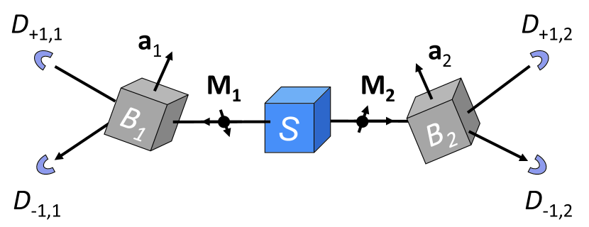
Figure 2: (Color online) Diagram of the EPRB thought experiment. The source $S$, activated at times labeled by $i=1,2,\ldots,N$, sends a particle with magnetic moment, represented by the unit vector $\mathbf{M_{1}}$, to the Stern-Gerlach magnet $B_{1}$ and another particle with magnetic moment, represented by the unit vector $\mathbf{M_{2}}$, to the Stern-Gerlach magnet $B_{2}$. The orientations of the magnets, represented by unit vectors $\mathbf{a_{1}}$ and $\mathbf{a_{2}}$, affect the deflection of the particles by the magnets. Each particle going to the left (right) is detected with 100% certainty by either $D_{+1,1}$ or $D_{-1,1}$ ($D_{+1,2}$ or $D_{-1,2}$).

3 Einstein-Podolsky-Rosen-Bohm thought experiment

In this section we repeat the analysis of Section 2 for Bohm’s version of the Einstein-Podolsky-Rosen thought experiment [42, 43]. The layout and description of the EPRB thought experiment is given in Fig. 2. The result of a run of the experiment for fixed $\mathbf{a}_{1}$ and $\mathbf{a}_{2}$ is a data set of pairs

$${\cal D} = \{(x_{1},y_{1}),\ldots,(x_{N},y_{N})|;x_{i}=\pm 1,y_{i}=\pm 1,\;i=1,\ldots,N\},$$ (23)

where $N$ is the total number of pairs emitted by the source. From the data set Eq. (23), we compute the numbers of coincidences

$$n_{xy}=\sum_{i=1}^{N}\delta_{x,x_{i}}\delta_{y,y_{i}}\quad,\quad x,y=\pm 1,$$ (24)

the averages

$$\langle x\rangle=\frac{1}{N}\sum_{i=1}^{N}x_{i}=\frac{n_{+1,+1}+n_{+1,-1}-n_{-1,+1}-n_{-1,-1}}{n_{+1,+1}+n_{+1,-1}+n_{-1,+1}+n_{-1,-1}}\quad,\quad\langle y\rangle=\frac{1}{N}\sum_{i=1}^{N}y_{i}=\frac{n_{+1,+1}+n_{-1,+1}-n_{+1,-1}-n_{-1,-1}}{n_{+1,+1}+n_{+1,-1}+n_{-1,+1}+n_{-1,-1}},$$ (25)

and the correlation

$$\langle xy\rangle = \frac{1}{N}\sum_{i=1}^{N}x_{i}y_{i}=\frac{n_{+1,+1}+n_{-1,-1}-n_{-1,+1}-n_{+1,-1}}{n_{+1,+1}+n_{+1,-1}+n_{-1,+1}+n_{-1,-1}}.$$ (26)

As in the case of the SG experiment, we assume that outcomes with different index $i$ are independent. In this case, the order in which the pairs appear from the source is irrelevant and we can compress/represent the content of the data set into/by the four numbers $n_{xy}$ for $x,y=\pm 1$. In other words, the frequencies

$$f(x,y|\mathbf{a}_{1},\mathbf{a}_{2},\mathbf{M}_{1},\mathbf{M}_{2},Z) = \frac{n_{xy}}{N}=\frac{1+x\langle x\rangle+y\langle y\rangle+xy\langle xy\rangle}{4},$$ (27)

provide a complete characterization of the data set Eq. (23) in terms of the three numbers $\langle x\rangle$, $\langle y\rangle$ and $\langle xy\rangle$.

Instead of continuing with the most general case it is, for pedagogical reasons, expedient to limit the discussion to the case which is relevant for the EPRB thought experiment. A first characteristic of the EPRB thought experiment is that the events $x_{i}$ and $y_{i}$ appear random and equally likely. This implies that $\langle x\rangle=\langle y\rangle=0$. A second characteristic is that the correlation $\langle xy\rangle$ does not depends on the orientation of the reference frame. This implies that $\langle xy\rangle$ must be a function of $\mathbf{a}_{1}\cdot\mathbf{a}_{2}$ only. Therefore, in this special but important case, Eq. (27) takes the form

$$f(x,y|\mathbf{a}_{1}\cdot\mathbf{a}_{2},Z) = \frac{n_{xy}}{N}=\frac{1+xyE(\mathbf{a}_{1}\cdot\mathbf{a}_{2},Z)}{4}=\frac{1+xyE(\theta,Z)}{4},$$ (28)

where $\cos\theta=\mathbf{a}_{1}\cdot\mathbf{a}_{2}$. As in the case of the SG experiment, on the basis of Eq. (28), there is no way to separate the description of the source emitting the particles from the description of the measurement process. In the subsection that follows, we demonstrate how the quantum theoretical description of the EPRB thought experiment naturally appears by separating the description of the data into source and measurement parts. In essence, we repeat the steps of Section 2.1 except that we have four ($x,y=\pm 1$) instead of two ($x=\pm 1$) possibilities to consider.

3.1 Separation procedure

In essence, the following is a straightforward extension of the procedure outlined in Section 2.1. We start by writing the observations $xy=(+1,-1,+1,-1)$ and $(f(+1,+1|\theta,Z)$, $f(-1,+1|\theta,Z)$, $f(+1,-1|\theta,Z)$, $f(-1,-1|\theta,Z))$ as $4\times 4$ matrices $X$ and $F$ with elements $X([x,y],[x^{\prime},y^{\prime}])=x\delta_{x,x^{\prime}}\delta_{y,y^{\prime}}$ and $Y([x,y],[x^{\prime},y^{\prime}])=y\delta_{x,x^{\prime}}\delta_{y,y^{\prime}}$ and $F([x,y],[x^{\prime},y^{\prime}])=f(xy|\mathbf{a},\mathbf{M},Z)\delta_{x,x^{\prime}}\delta_{y,y^{\prime}}$, respectively. Here we use the notation $[x,y]=(1-x)/2+(1-y)$ to indicate that the pairs $(x,y)$ and $(x^{\prime},y^{\prime})$ specify the row, respectively the column index (running from 0 to 3) of the matrices $X$ and $F$. We require that

$$\mathbf{Tr}\widehat{\rho}=1\quad,\quad\mathbf{Tr}\widehat{\rho}\widehat{X}=\langle x\rangle\quad,\quad\mathbf{Tr}\widehat{\rho}\widehat{Y}=\langle y\rangle\quad,\quad\mathbf{Tr}\widehat{\rho}\widehat{X}\widehat{Y}=\langle xy\rangle.$$ (29)

where instead of the $2\times 2$ matrices in the SG case, we now look for $4\times 4$ matrices $\widehat{\rho}$, $\widehat{X}$, and $\widehat{Y}$ which satisfy Eq. (29) but allow for the desired separation. From linear algebra we know that any hermitian $4\times 4$ matrix can be written as a linear combination of sixteen hermitian $4\times 4$ matrices. These sixteen matrices may be chosen such that they are orthonormal with respect to the inner product defined by $(A,B)=\mathbf{Tr\;}A^{\dagger}B$. Using the direct product of the Pauli-spin matrices $\bm{\sigma}_{j}=(\sigma^{x}_{j},\sigma^{y}_{j},\sigma^{z}_{j})$ for $j=1,2$ and the unit matrix 11 as the orthonormal basis set for the vector space of $4\times 4$ matrices, we may write (without loss of generality)

$$\widehat{\rho} = \rho_{0}\leavevmode\hbox{\small 1\normalsize\kern-3.30002pt1}+\bm{\rho}_{1}\cdot\bm{\sigma}_{1}\otimes\leavevmode\hbox{\small 1\normalsize\kern-3.30002pt1}_{2}+\leavevmode\hbox{\small 1\normalsize\kern-3.30002pt1}_{1}\otimes\bm{\rho}_{2}\cdot\bm{\sigma}_{2}+\bm{\sigma}_{1}\cdot\bm{\rho}_{12}\cdot\bm{\sigma}_{2}.$$ (30)

where the number $\rho_{0}$, the vectors $\bm{\rho}_{j}$, and the matrix $\bm{\rho}_{12}$ are all real-valued. As each of the two sides of the EPRB experiment contains a SG magnet, consistency with the separated description of the SG experiment demands that we choose

$$\widehat{X}=\mathbf{a}_{1}\cdot\bm{\sigma}_{1}\otimes\leavevmode\hbox{\small 1\normalsize\kern-3.30002pt1}_{2}\quad,\quad\widehat{Y}=\leavevmode\hbox{\small 1\normalsize\kern-3.30002pt1}_{1}\otimes\mathbf{a}_{2}\cdot\bm{\sigma}_{2}.$$ (31)

We find the explicit expression of $\widehat{\rho}$ by requiring that Eq. (29) holds. Focussing on the case of the EPRB experiment for which $\langle x\rangle=\langle y\rangle=0$ and $\langle xy\rangle=-\mathbf{a}_{1}\cdot\mathbf{a}_{2}$, it readily follows that $\rho_{0}=1/4$, $\bm{\rho}_{1}=\bm{\rho}_{2}=0$ and that $\widehat{\rho}$ takes the form

$$\widehat{\rho} = \frac{\leavevmode\hbox{\small 1\normalsize\kern-3.30002pt1}-\sigma_{1}\cdot\sigma_{2}}{4}.$$ (32)

It is not difficult to verify that ${\widehat{\rho}}^{2}={\widehat{\rho}}$, hence, in quantum parlance, Eq. (32) is the density matrix of a pure quantum state [39]. Computing the matrix elements of ${\widehat{\rho}}$ in the spin-up, spin-down basis of both spins we find

$$\widehat{\rho} = \left(\frac{|\uparrow\downarrow\rangle-|\downarrow\uparrow\rangle}{\sqrt{2}}\right)\left(\frac{\langle\uparrow\downarrow|-\langle\downarrow\uparrow|}{\sqrt{2}}\right),$$ (33)

and

$$\langle xy\rangle = \mathbf{Tr\;}\widehat{\rho}\widehat{X}\widehat{Y}=\mathbf{Tr\;}\widehat{\rho}\mathbf{a}_{1}\cdot\bm{\sigma}_{1}\mathbf{a}_{2}\cdot\bm{\sigma}_{2}=-\mathbf{a}_{1}\cdot\mathbf{a}_{2},$$ (34)

which we recognize as the quantum theoretical description of two spin-1/2 objects in the singlet state.

In other words, we have shown that rewriting the data gathered in an ideal EPRB thought experiment in a manner that allows for the envisaged separation naturally leads, without invoking postulates of quantum theory, to the quantum theoretical problem of two $S=1/2$ spins in the singlet state.

As in the case of the ideal SG experiment, the separated representation Eq. (31) and Eq. (32) puts a severe restriction on the kind of data that we can describe, again provoking to question “what is so special about the case in which the separation procedure can be carried out?” In the next subsection, we answer this question in terms of a LI treatment of robust EPRB experiments [2].

3.2 Logical-inference treatment

A detailed account of the LI treatment of the EPRB thought experiment can be found in Ref. [2]. Moreover, as the LI treatment of the EPRB thought experiment is, in essence, the same as the one of the idealized SG experiment given in Section 2.2, we limit the presentation to a discussion of the assumptions and the results.

1. The i-prob to observe a pair $\{x,y\}$ is denoted by $P(x,y|\mathbf{a}_{1},\mathbf{a}_{2},Z)$ where $Z$ represents all the conditions under which the experiment is performed, with exception of the directions $\mathbf{a}_{1}$ and $\mathbf{a}_{2}$ of the magnets $B_{1}$ and $B_{2}$, respectively. It is assumed that the conditions represented by $Z$ are fixed and identical for all experiments. Note that we have omitted the (in)dependence on $M_{1}$ and $M_{2}$ because in the case at hand, it is redundant [2].

2. For simplicity, it is assumed that there is no relation between the actual values of the pairs $\{x_{n},y_{n}\}$ and $\{x_{n^{\prime}},y_{n^{\prime}}\}$ if $n\not=n^{\prime}$, meaning that each repetition of the experiment represents an identical event of which the outcome is logically independent of any other such event. Invoking the product rule, the logical consequence of this assumption is that

   $$P(x_{1},y_{1},\ldots,x_{N},y_{N}|\mathbf{a}_{1},\mathbf{a}_{2},Z) = \prod_{i=1}^{N}P(x_{i},y_{i}|\mathbf{a}_{1},\mathbf{a}_{2},Z),$$ (35)

   meaning that the i-prob $P(x_{1},y_{1},\ldots,x_{N},y_{N}|\mathbf{a}_{1},\mathbf{a}_{2},Z)$ to observe the compound event $\left\{\{x_{1},y_{1}\},\ldots,\{x_{N},y_{N}\}\right\}$ is completely determined by the i-prob $P(x,y|\mathbf{a}_{1},\mathbf{a}_{2},Z)$ to observe the pair $\{x,y\}$.

3. It is assumed that the i-prob $P(x,y|\mathbf{a}_{1},\mathbf{a}_{2},Z)$ to observe a pair $\{x,y\}$ does not change if we apply the same rotation to both magnets $B_{1}$ and $B_{2}$. Expressing this invariance with respect to rotations of the coordinate system (Euclidean space and Cartesian coordinates are used throughout this paper) in terms of i-probs requires that $P(x,y|\mathbf{a}_{1},\mathbf{a}_{2},Z)=P(x,y|{\cal R}\mathbf{a}_{1},{\cal R}\mathbf{a}_{2},Z)$ where ${\cal R}$ denotes an arbitrary rotation in three-dimensional space which is applied to both magnets $B_{1}$ and $B_{2}$. As a function of the vectors $\mathbf{a}_{1}$ and $\mathbf{a}_{2}$, the functional equation $P(x,y|\mathbf{a}_{1},\mathbf{a}_{2},Z)=P(x,y|{\cal R}\mathbf{a}_{1},{\cal R}\mathbf{a}_{2},Z)$ can only be satisfied for all $\mathbf{a}_{1}$, $\mathbf{a}_{2}$ and rotations ${\cal R}$ if $P(x,y|\mathbf{a}_{1},\mathbf{a}_{2},Z)$ is a function of the inner product $\mathbf{a}_{1}\cdot\mathbf{a}_{2}$ only. Therefore, we must have

   $$P(x,y|\mathbf{a}_{1},\mathbf{a}_{2},Z)=P(x,y|\mathbf{a}_{1}\cdot\mathbf{a}_{2},Z)=P(x,y|\theta,Z),$$ (36)

   where $\theta=\arccos(\mathbf{a}_{1}\cdot\mathbf{a}_{2})$ denotes the angle between the unit vectors $\mathbf{a}_{1}$ and $\mathbf{a}_{2}$. For any integer value of $K$, $\theta+2\pi K$ represents the same physical arrangement of the magnets $M_{1}$ and $M_{2}$.

4. From the LI rules, it follows that the i-prob to observe $x$, irrespective of the observed value of $y$ is given by

   $$P(x|\mathbf{a}_{1},\mathbf{a}_{2},Z)=\sum_{y=\pm 1}P(x,y|\mathbf{a}_{1},\mathbf{a}_{2},Z).$$ (37)

   The assumption that observing $x=+1$ is as likely as observing $x=-1$, independent of the observed value of $y$, implies that we must have $P(x=+1|\mathbf{a}_{1},\mathbf{a}_{2},Z)=P(x=-1|\mathbf{a}_{1},\mathbf{a}_{2},Z)$ which, in view of the fact that $P(x=+1|\mathbf{a}_{1},\mathbf{a}_{2},Z)+P(x=-1|\mathbf{a}_{1},\mathbf{a}_{2},Z)=1$ implies that $P(x=+1|\mathbf{a}_{1},\mathbf{a}_{2},Z)=P(x=-1|\mathbf{a}_{1},\mathbf{a}_{2},Z)=1/2$. Applying the same reasoning to the assumption that, independent of the observed values of $x$, observing $y=+1$ is as likely as observing $y=-1$ yields $P(y|\mathbf{a}_{1},\mathbf{a}_{2},Z)=P(x=+1,y|\mathbf{a}_{1},\mathbf{a}_{2},Z)+P(x=-1,y|\mathbf{a}_{1},\mathbf{a}_{2},Z)=1/2$.

Note that we did not assign any prior i-prob nor did we make any reference to concepts such as the singlet-state. Although the symmetry properties which have been assumed are reminiscent of those of the singlet state, this is deceptive: without altering the assumptions that are expressed in (3) and (4), the LI approach yields the correlations for the triplet states as well [2].

Adopting the same reasoning as in Section 2.2, it follows directly from assumptions (1–4) that the i-prob to observe a pair $\{x,y\}$ takes the form [2]

$$P(x,y|\theta,Z)=\frac{1+xyE_{12}(\theta)}{4},$$ (38)

where $E_{12}(\theta)=E_{12}(\mathbf{a}_{1},\mathbf{a}_{2},Z)$ is a periodic function of $\theta$. Minimization of the corresponding expression of $|\mathrm{Ev}|$ while taking into account the constraints (C2) and (C3) (see Section 2.2) is tantamount to finding the i-prob’s $P(x,y|\theta,Z)$ which minimize [2]

$$I_{F}=\sum_{x,y=\pm 1}\frac{1}{P(x,y|\theta,Z)}\left(\frac{\partial P(x,y|\theta,Z)}{\partial\theta}\right)^{2},$$ (39)

subject to the constraint that $\partial P(x,y|\theta,Z)/\partial\theta\not=0$ for some pairs $(x,y)$. The r.h.s. of Eq. (39) is the Fisher information for the problem at hand and because of constraint (C3), does not depend on $\theta$. Using Eq. (38), we can rewrite Eq. (39) as

$$I_{F}=\frac{1}{1-E_{12}^{2}(\theta)}\left(\frac{\partial E_{12}(\theta)}{\partial\theta}\right)^{2},$$ (40)

which is readily integrated to yield $E_{12}(\theta)=\cos\left(\theta\sqrt{I_{F}}+\phi\right)$ where $\phi$ is an integration constant. As $E_{12}(\theta)$ is a periodic function of $\theta$ we must have $\sqrt{I_{F}}=K$ where $K$ is an integer and hence

$$E_{12}(\theta)=\cos\left(K\theta+\phi\right).$$ (41)

Because of constraint (C2) we exclude the case $K=I_{F}=0$ from further consideration because it describes an experiment in which the frequency distribution of the observed data does not depend on $\theta$. Therefore, the physically relevant, nontrivial solution with minimum Fisher information corresponds to $K=1$. Furthermore, as $E_{12}(\theta)$ is a function of $\mathbf{a}_{1}\cdot\mathbf{a}_{2}=\cos\theta$ only, we must have $\phi=0,\pi$, reflecting an ambiguity in the definition of the direction of $B_{1}$ relative to the direction of $B_{2}$.

Choosing the solution with $\phi=\pi$, the two-particle i-prob reads

$$P(x,y|\mathbf{a}_{1},\mathbf{a}_{2},Z)=\frac{1+xy\mathbf{a}_{1}\cdot\mathbf{a}_{2}}{4}\quad,\quad\sum_{x,y=\pm 1}xyP(x,y|\mathbf{a}_{1},\mathbf{a}_{2},Z)=\langle xy\rangle=-\mathbf{a}_{1}\cdot\mathbf{a}_{2},$$ (42)

in agreement with the expression for the correlation of two $S=1/2$ particles in the singlet state [43, 39]. We may therefore conclude that without making reference to concepts of quantum theory, the LI treatment of the robust EPPB experiment directly yields the probabilistic description that we know from quantum theory. This demonstrates that the data produced by EPRB experiments can be described, in a more general manner, without invoking the notion of quantum entanglement.

3.3 Discussion

In Section 3.1 we apply the separating procedure to the EPRB thought experiment and demonstrate how the quantum theoretical description in terms of the singlet state emerges from a simple rearrangement of the representation of the data.

Section 3.2 shows that the application of the criterion of robust, reproducible experiments [2] to the EPRB thought experiment depicted in Fig. 2 amounts to minimizing the Fisher information Eq. (40) for this specific problem. The result of this calculation is Eq. (42), the probability distribution that is characteristic for two spin-1/2 objects in the singlet state. Needless to say, the derivation that led to Eq. (42) did not require invoking concepts of quantum theory. Only rational reasoning strictly complying with the rules of LI and some elementary facts about the experiment were used.

It is most remarkable that the quantum theoretical description of a system in the singlet state emerges by simply requiring that (i) everything which is known about the source is uncertain, except that it emits two signals, (ii) the magnets $B_{1}$ and $B_{2}$ transform the received signal into two-valued signals, and that (iii) the i-prob describing the frequencies of the pair of events $(x,y)$ does not depend on the orientation of the reference frame [2]. We emphasize that Sections 3.1 and 3.2 address different ways of representing frequencies of two-valued data obtained in robust experiments and have no bearing on the issue non-locality as such.

In spite of the widely spread claims that real EPRB experiments have proven quantum theory correct, it is a fact that none of the three different experiments for which data has been made available [44, 45, 46] survives the confrontation with the 5-standard-deviation-criterion hypothesis test that the data complies with the quantum theoretical description Eq. (42) [47]. It seems that for the time being, only computer experiments are able to generate data that are not in conflict with the quantum theoretical description of the EPRB thought experiment [47].

4 Relation to previous work

4.1 Subject-object separation

The general issue of separating subject and object or more specifically, the limitations on the separation of the phenomenon under scrutiny from the process of gathering data about it have played an important role in the development of quantum physics [48, 40, 49, 50]. In this context, the typical signatures of quantum physics appear as result of the impossibility to gather data about the (atomic) objects without significantly disturbing their behavior. While this viewpoint is implicit in the LI derivation of equations such as the Schrödinger equation [1, 2, 3], in our view, the separation procedure discussed in the present paper does not really address this issue. The separation procedure explores alternatives for representing data sets and selects the quantum theoretical description as the representation in which the various parts of the experiment that may affect the data production process appear as independent entities, in sharp contrast with the original representation of the data set in terms of frequencies. On the other hand, there is a relation between the notion of “complementarity” advocated by N. Bohr [48, 40, 49, 50] and the separation procedure discussed in the present paper.

For simplicity, we discuss this issue using the SG experiment as an example but without modification, the arguments carry over to the EPRB experiment as well. Suppose that we want to describe the outcomes of two SG experiments with two different settings $\mathbf{a}\not=\mathbf{b}$. Obviously, in practice we cannot perform the experiment with $\mathbf{a}$ and $\mathbf{b}$ at the same time: the two conditions are mutually exclusive. On the level of the description in terms of the frequency Eq. (3), we require the specification of two numbers $E(\mathbf{a},\mathbf{M},Z)$ and $E(\mathbf{b},\mathbf{M},Z)$. In general, there is no principle, in fact no reason at all, that would enforce a relation between these two numbers: a full characterization of the experiment in terms of classical concepts (the directions $\mathbf{a}$ and $\mathbf{M}$) would require data of $E(\mathbf{a},\mathbf{M},Z)$ for all $\mathbf{a}$ (for simplicity we assume that $\mathbf{M}$ is fixed). But once we require that the separation procedure can be carried out, the matrix calculus that is characteristic of quantum theory emerges and the resulting formalism in terms of non-commuting matrices allows for one common description of all possible mutually exclusive experiments. Apparently, the conditions for which Bohr’s statement[48] “an adequate tool for a complementary way of description is offered precisely by the quantum-mechanical formalism which represents a purely symbolic scheme permitting only predictions, on lines of the correspondence principle, as to results obtainable under conditions specified by means of classical concepts” holds correspond to those for which the separation procedure can be carried out.

4.2 Gleason-Bush theorem

The Gleason-Bush theorem [51, 52] assumes that there is a (finite) Hilbert space, with “events” being defined to be closed subspaces of this Hilbert space. One then considers the algebra of these “events” and defines a map (a kind of “probability”) on this algebra, mapping events to real numbers. The theorem then says that this map must have the structure $\langle\mathbf{v}|\rho|\mathbf{v}\rangle$ where $\mathbf{v}$ represents one of the “events” and $\rho$ is a density matrix. The key point is that the algebra dictates the structure of the map (i.e. Born’s rule). Based on these considerations, Pitowsky suggests that the Hilbert space formalism of quantum mechanics is a new theory of probability [53] and continues to state that “The quantum structure is in this sense much more constrained than the classical formalism. The structure of the phase space of a classical system does not greatly restrict the type of probability measures that can be defined on it. The probability measures which are actually used in classical statistical mechanics are introduced mostly by fiat or, in any case, are very hard to justify.” This line of thinking is orthogonal to the one adopted in the present paper in which events are not restricted to be “closed subspaces of some Hilbert space”. By way of concrete examples, the present paper shows that the Hilbert space formalism emerges from the desire to separate the description into various parts and that the quantum theoretical description is indeed a constrained form of probability theory.

5 Summary

In Section 2.1, the quantum theoretical description of the idealized SG experiment is shown to derive by separating the representation of the observed data into a description of the object under study and a description of the measurement device. Section 2.2 shows that the class of experimental outcomes which can be described by quantum theory are special in the sense that they are the results of a robust Stern-Gerlach experiment [2].

Section 3.1 demonstrates that the quantum theoretical description of the Einstein-Podolsky-Rosen-Bohm thought experiment naturally emerges by separating the representation of the observed data into a description of the object under study and a description of the measurement device. As the logical-inference derivation of Section 3.2 yields the same expressions, it also follows that the class of experiments which quantum theory can describe is smaller than the one which allows a description in terms of conditional probabilities.

The answer to the question “what is so special about the case in which the separation procedure can be carried out and under which conditions can quantum theory be used to describe the statistical experiment?” is the same for both the Stern-Gerlach and Einstein-Podolsky-Rosen-Bohm thought experiment, namely that the experimental data which quantum theory can describe are special in the sense that they are the result of a robust experiment [2]. Once we accept as a principle, the idea of separation in the sense explained in Section 2.1, the representation of the data in terms of quantum theoretical constructs is completely determined by the rules of linear algebra, i.e. by mathematics alone.

Although logical-inference applied to a different class of robust experiments as those discussed in the present paper lead to the Schrödinger and Pauli equation [1, 2, 3], in the current formulation there is nothing to separate: there is only a data set of clicks of detectors and the no control over the unknown position of the particle [2, 3]. Extending the application of the separation procedure to these more complicated cases is left for future research.

References

- [1] H. De Raedt, M. I. Katsnelson, and K. Michielsen, “Quantum theory as the most robust description of reproducible experiments: application to a rigid linear rotator,” Proc. SPIE 8832, pp. 883212–1–11, 2013.
- [2] H. De Raedt, M. I. Katsnelson, and K. Michielsen, “Quantum theory as the most robust description of reproducible experiments,” Ann. Phys. 347, pp. 45 – 73, 2014.
- [3] H. De Raedt, M. I. Katsnelson, H. C. Donker, and K. Michielsen, “Quantum theory as a description of robust experiments: derivation of the Pauli equation,” Ann. Phys. 359, pp. 166 – 186, 2015.
- [4] R. T. Cox, “Probability, Frequency and Reasonable Expectation,” Am. J. Phys. 14, pp. 1 – 13, 1946.
- [5] R. T. Cox, The Algebra of Probable Inference, Johns Hopkins University Press, Baltimore, 1961.
- [6] M. Tribus, Rational Descriptions, Decisions and Designs, Expira Press, Stockholm, 1999.
- [7] C. R. Smith and G. Erickson, “From Rationality and consistency to Bayesian probability,” in Maximum Entropy and Bayesian Methods, J. Skilling, ed., pp. 29 – 44, Kluwer Academic Publishers, (Dordrecht), 1989.
- [8] E. T. Jaynes, Probability Theory: The Logic of Science, Cambridge University Press, Cambridge, 2003.
- [9] A. Y. Khrennikov, Contextual Approach to Quantum Formalism, Springer, Berlin, 2009.
- [10] D. Home, Conceptual Foundations of Quantum Physics, Plenum Press, New York, 1997.
- [11] L. E. Ballentine, “Interpretations of Probability and Quantum Theory,” in Foundations of Probability and Physics, A. Khrennikov, ed., pp. 71 – 84, World Scientific, (Singapore), 2001.
- [12] R. B. Griffiths, Consistent Quantum Theory, Cambridge University Press, Cambridge, 2002.
- [13] J. Pearl, Causality: models, reasoning, and inference, Cambridge University Press, Cambridge, 2000.
- [14] A. Plotnitsky, ““Dark Materials to Create More Worlds”: On Causality in Classical Physics, Quantum Physics, and Nanophysics,” J. Comput. Theor. Nanosci. 8, pp. 983 – 997, 2011.
- [15] K. De Raedt, H. De Raedt, and K. Michielsen, “Deterministic event-based simulation of quantum interference,” Comp. Phys. Comm. 171, pp. 19 – 39, 2005.
- [16] K. Michielsen, F. Jin, and H. De Raedt, “Event-based corpuscular model for quantum optics experiments,” J. Comput. Theor. Nanosci. 8, pp. 1052 – 1080, 2011.
- [17] H. De Raedt and K. Michielsen, “Event-by-event simulation of quantum phenomena,” Ann. Phys. (Berlin) 524, pp. 393 – 410, 2012.
- [18] H. De Raedt, F. Jin, and K. Michielsen, “Event-based simulation of neutron interferometry experiments,” Quantum Matter 1, pp. 1 – 21, 2012.
- [19] H. De Raedt and K. Michielsen, “Discrete-event simulation of uncertainty in single-neutron experiments,” Frontiers in Physics 2(14), 2014.
- [20] K. Michielsen and H. De Raedt, “Event-based simulation of quantum physics experiments,” Int. J.. Mod. Phys. C 25, p. 01430003, 2014.
- [21] A. E. Allahverdyan, R. Balian, and T. M. Nieuwenhuizen, “Understanding quantum measurement from the solution of dynamical models,” Phys. Rep. 525, pp. 1 – 166, 2013.
- [22] A. Khrennikov, Ubiquitous Quantum Structure: From Psychology to Finance, Springer Berlin Heidelberg, 2010.
- [23] J. P. Ralston, “Emergent mechanics, quantum and un-quantum,” Proc. SPIE 8832, pp. 88320W1–25, 2013.
- [24] L. de la Peña, A. M. Cetto, and T. A. Brody, “On hidden-variable theories and Bell’s inequality,” Lett. Nuovo Cim. 5, pp. 177 – 181, 1972.
- [25] A. Fine, “On the completeness of quantum theory,” Synthese 29, pp. 257 – 289, 1974.
- [26] T. Brody, The Philosphy Behind Physics, Springer, Berlin, 1993.
- [27] M. Kupczyński, “On some tests of completeness of quantum mechanics,” Phys. Lett. A 116, pp. 417 – 419, 1986.
- [28] E. T. Jaynes, “Clearing up mysteries - The original goal,” in Maximum Entropy and Bayesian Methods, J. Skilling, ed., 36, pp. 1 – 27, Kluwer Academic Publishers, (Dordrecht), 1989.
- [29] L. Sica, “Bell’s inequalities I: An explanation for their experimental violation,” Opt. Comm. 170, pp. 55 – 60, 1999.
- [30] K. Hess and W. Philipp, “Bell’s theorem and the problem of decidability between the views of Einstein and Bohr,” Proc. Natl. Acad. Sci. USA 98, pp. 14228 – 14233, 2001.
- [31] K. Hess and W. Philipp, “Bell’s theorem: Critique of proofs with and without inequalities,” AIP Conf. Proc. 750, pp. 150 – 157, 2005.
- [32] A. F. Kracklauer, “Bell’s inequalities and EPR-B experiments: Are they disjoint?,” AIP Conf. Proc. 750, pp. 219 – 227, 2005.
- [33] E. Santos, “Bell’s theorem and the experiments: Increasing empirical support to local realism?,” Stud. Hist. Phil. Mod. Phys. 36, pp. 544 – 565, 2005.
- [34] T. M. Nieuwenhuizen, “Where Bell went wrong,” AIP Conf. Proc. 1101, pp. 127 – 133, 2009.
- [35] K. Hess, K. Michielsen, and H. De Raedt, “Possible experience: from Boole to Bell,” Europhys. Lett. 87, p. 60007, 2009.
- [36] T. M. Nieuwenhuizen, “Is the contextuality loophole fatal for the derivation of Bell inequalities?,” Found. Phys. 41, pp. 580 – 591, 2011.
- [37] H. De Raedt, K. Hess, and K. Michielsen, “Extended Boole-Bell inequalities applicable to quantum theory,” J. Comput. Theor. Nanosci. 8, pp. 1011 – 1039, 2011.
- [38] K. Hess, Einstein Was Right!, Pan Stanford Publishing, Singapore, 2015.
- [39] L. E. Ballentine, Quantum Mechanics: A Modern Development, World Scientific, Singapore, 2003.
- [40] N. Bohr, “XV. The Unity of Human Knowledge,” in Complementarity Beyond Physics (1928 –1962), D. Favrholdt, ed., Niels Bohr Collected Works 10, pp. 155 – 160, Elsevier, Amsterdam, 1999.
- [41] “For additional information see.” .
- [42] A. Einstein, A. Podolsky, and N. Rosen, “Can quantum-mechanical description of physical reality be considered complete?,” Phys. Rev. 47, pp. 777 – 780, 1935.
- [43] D. Bohm, Quantum Theory, Prentice-Hall, New York, 1951.
- [44] G. Weihs, Ein Experiment zum Test der Bellschen Ungleichung unter Einsteinscher Lokalität. PhD thesis, University of Vienna, 2000. .
- [45] Y. Shih, An Introduction to Quantum Optics: Photon and Biphoton Physics, CRC Press, Boca Raton, 2011.
- [46] A. Vistnes and G. Adenier, “There may be more to entangled photon experiments than we have appreciated so far,” AIP Conf. Proc. 1508, pp. 326 – 333, 2012.
- [47] H. De Raedt, F. Jin, and K. Michielsen, “Data analysis of Einstein-Podolsky-Rosen-Bohm laboratory experiments,” Proc. SPIE 8832, pp. 88321N1–11, 2013.
- [48] N. Bohr, “Discussion with Einstein on epistemological problems in atomic physics,” in A. Einstein. Autobiographical Notes. A Centennial Edition., P. A. Schilpp, ed., Open Court, (La Salle, Illinois), 1979.
- [49] A. Plotnitsky, ”Epistemology and Probability: Bohr, Heisenberg, Schrödinger, and the Nature of Quantum-Theoretical Thinking”, Springer, Berlin, 2010.
- [50] A. Plotnitsky, Niels Bohr and Complementarity: An introduction, Springer, Berlin, 2013.
- [51] A. Gleason, “Measures on the closed subspaces of a Hilbert space,” J. Math. Mech. 6, p. 887, 1957.
- [52] P. Busch, “Quantum states and generalized observables: A simple proof of Gleason’s theorem,” Phys. Rev. Lett. 91, p. 120403, 2003.
- [53] I. Pitowsky, “Quantum mechanics as a theory of probability,” in Physical Theory and its Interpretation, W. Demopoulos and I. Pitowsky, eds., The Western Ontario Series in Philosophy of Science 72, pp. 213–240, Springer Netherlands, 2006.