Numerical Solution of the Robin Problem of Laplace Equations with a Feynman-Kac Formula and Reflecting Brownian Motions

Abstract

In this paper, we present numerical methods to implement the probabilistic representation of third kind (Robin) boundary problem for the Laplace equations. The solution is based on a Feynman-Kac formula for the Robin problem which employs the standard reflecting Brownian motion (SRBM) and its boundary local time arising from the Skorohod problem. By simulating SRBM paths through Brownian motion using Walk on Spheres (WOS) method, approximation of the boundary local time is obtained and the Feynman-Kac formula is calculated by evaluating the average of all path integrals over the boundary under a measure defined through the local time. Numerical results demonstrate the accuracy and efficiency of the proposed method for finding a local solution of the Laplace equations with Robin boundary conditions.

,

1 Introduction

Partial differential equations (PDEs) have been widely used to describe a variety of phenomena such as electrostatics, electrodynamics, fluid flow or quantum mechanics. Traditionally, finite difference, finite element and boundary element methods are the mainstream numerical approaches to solve the PDEs. Recently, using the Feynman-Kac formula [5][6][7] which connects solutions of differential equations of diffusion and heat flow and random processes of Brownian motions, numerical methods based on random walks or Monte Carlo diffusions have been explored for solving parabolic and elliptic PDEs [11][25].

The Feynman-Kac formula represents the solutions of parabolic and elliptic PDEs as the expectation functionals of stochastic processes (specifically Brownian motions), and conversely, the probabilistic properties of diffusion processes can be obtained through investigating related PDEs characterized by corresponding generators [22]. The formula involves the path integrals of the diffusion process starting from an arbitrarily prescribed location, and this enables us to find a local numerical solution without constructing space and time meshes as in traditional deterministic numerical methods mentioned above, which incur expensive costs in high dimensions. In many applications it is also of practical importance and necessity to seek a local solution of PDEs at some interested points. If the sample paths of a diffusion process are simulated, then by computing the average of path integrals we can obtain approximations to the exact solutions of the PDEs. For second order elliptic PDEs with Dirichlet and Neumann boundaries, the average of path integrals is reduced to the average of boundary integrals under certain measure where the detailed trajectories of the diffusion process have no effect on the averages except the hitting locations on the boundaries.

Simulations of diffusion paths can be done by random walks methods [3][8] [11] [13] either on lattice or in continuum space. In some cases such as for the Poisson equation, the Feynman-Kac formula has a pathwise integral requiring the detailed trajectory of each path. Moreover, one may need to adopt random walks on a discrete lattice in order to incorporate inhomogeneous source terms. As for the continuum space approach, the Walk on Spheres (WOS) method is preferred where the path of diffusion process within the domain does not appear in the Feynman-Kac formula. For both approaches, the geometry of the boundaries need special care for accurate results [14]. In our previous work on Laplace equation with Neumann boundary conditions [4], we proposed a numerical method to simulate the standard reflecting Brownian motion (SRBM) path using WOS and obtained the boundary local time of the SRBM. As a result, a local numerical solution of the PDE is achieved by using the Feynman-Kac formula. Other literatures [9][10][13][14] have also explored similar problems. Especially, in [13] schemes based on the WOS, Euler schemes and kinetic approximations are proposed to treat inhomogeneous Neumann problems. It turns out that the pointwise resolution is much harder due to the choice of the truncation of time. However, the local time was not handled explicitly in [13]. On the other hand, Monte Carlo simulations were discussed in [14] where the positive part of the boundary needs to be identified first. In this paper, following [4] we continue the use of SRBM to solve Robin boundary problems for the Laplace operator, which has many applications in heat transfer and impedance tomograph. Our goal again is to obtain a local approximation to the exact solution of the Robin problem.

The rest of paper is organized as follows. Firstly, the Skorohod problem is introduced in section 2, where both the concepts of standard reflecting Brownian motion and boundary local time will be reviewed briefly. This lays the foundation for the underlying diffusion process of the Robin boundary problem and the sampling of the diffusion paths. Secondly, an overview of the Feynamn-Kac formula is given in section 3. Thirdly, the probabilistic representation of the solution for the Robin boundary value problem proposed in [2][12] is discussed in section 4, and we will see the relation between the Neumann and Robin problems and gain a new perspective. Section 5 presents the numerical approaches and test results. Finally, conclusions and future work are given in section 6.

2 Skorohod problem, SRBM and boundary local time

Assume that $\displaystyle D$ is a domain with a $\displaystyle C^{1}$ boundary in $\displaystyle R^{3}$. The generalized Skorohod problem is stated as follows:

Definition 1

Let $\displaystyle f\in C([0,\infty),R^{3})$, a continuous function from $\displaystyle[0,\infty]$ to $\displaystyle R^{3}$. A pair $\displaystyle(\xi_{t},L_{t})$ is a solution to the Skorohod equation $\displaystyle S(f;D)$ if

1. $\displaystyle\xi$ is continuous in $\displaystyle\bar{D}$;

2. $\displaystyle L(t)$ is a nondecreasing function which increases only when $\displaystyle\xi\in\partial D$, namely,

   $$L(t)=\int_{0}^{t}I_{\partial D}(\xi(s))L(ds);$$ (2.1)

3. The Skorohod equation holds:

   $$S(f;D):\qquad\ \xi(t)=f(t)-\frac{1}{2}\int_{0}^{t}n(\xi(s))L(ds),$$ (2.2)

   where $\displaystyle n(x)$ denotes the outward unit normal vector at $\displaystyle x\in\partial D$.

The Skorohod problem was first studied in [1] by A.V. Skorohod in addressing the construction of paths for diffusion processes with boundaries, which results from the instantaneous reflection behavior of the processes at the boundaries. Skorohod presented the result in one dimension in the form of an Ito integral and Hsu [12] later extended the concept to $\displaystyle d$-dimensions ($\displaystyle d\geq 2$).

In the simple case that $\displaystyle D=[0,\infty)$, the solution to the Skorohod problem uniquely exists and can be explicitly given by

$$\centering\xi(t)=\left\{\begin{aligned} &f(t),&if\ t\leq\tau;\\ &f(t)-\inf_{\tau\leq s\leq t}f(s),&if\ t>\tau;\\ \end{aligned}\right.\@add@centering$$ (2.3)

where $\displaystyle\tau=\inf\left\{t>0:f(t)<0\right\}$. In general, solvability of the Skorohod problem is closely related to the smoothness of the domain $\displaystyle D$. For higher dimensions, the existence of (2.2) is guranteed for $\displaystyle C^{1}$ domains while uniqueness can be acheived for a $\displaystyle C^{2}$ domain by assuming the convexity for the domain [15]. Later, it was shown by Lions and Sznitman [16] that the constraints on $\displaystyle D$ can be relaxed to some locally convex properties.

Next we introduce the concept of SRBM and boundary local time which play important roles in solving Robin boundary problem by probabilistic approaches.

Suppose that $\displaystyle f(t)$ is a standard Brownian motion (SBM) starting at $\displaystyle x\in\bar{D}$ and $\displaystyle(X_{t},L_{t})$ is the solution to the Skorohod problem $\displaystyle S(f;D)$, then $\displaystyle X_{t}$ will be the standard reflecting Brownian motion (SRBM) on $\displaystyle D$ starting at $\displaystyle x$. Because the transition probability density of the SRBM satisfies the same parabolic differential equation as that by a BM, a sample path of the SRBM can be simulated simply as that of  the BM within the domain. However, the zero Neumann boundary condition for the density of SRBM implies that the path be pushed back at the boundary along the inward normal direction whenever it attempts to cross the latter. The full construction of a SRBM from a SBM can be found in our previous work [4].

The boundary local time $\displaystyle L_{t}$ is not an independent process but associated with SRBM $\displaystyle X_{t}$ and defined by

$$L(t)\equiv\lim_{\epsilon\rightarrow 0}\frac{\int_{0}^{t}I_{D_{\epsilon}}(X_{s})ds}{\epsilon},$$ (2.4)

where $\displaystyle D_{\epsilon}$ is a strip region of width $\displaystyle\epsilon$ containing $\displaystyle\partial D$ and $\displaystyle D_{\epsilon}\subset\overline{D}$. Here $\displaystyle L_{t}$ is called the local time of $\displaystyle X_{t}$, a notion invented by P. Lévy [23]. This limit exists both in $\displaystyle L^{2}$ and $\displaystyle P^{x}$-$\displaystyle a.s$. for any $\displaystyle x\in\overline{D}$.

It is obvious that $\displaystyle L_{t}$ measures the amount of time that the standard reflecting Brownian motion $\displaystyle X_{t}$ spends in a vanishing neighborhood of the boundary within the time period $\displaystyle[0,t]$. Besides, it is the unique continuous nondecreasing process that appears in the Skorohod equation. An interesting part of (2.4) is that the set $\displaystyle\left\{t\in R_{+}:X_{t}\in\partial D\right\}$ has a zero Lebesgue measure while the sojourn time of the set is nontrivial [23]. This concept is not just a mathematical one but also has physical relevance in understanding the “crossover exponent” associated with “renewal rate” in modern renewal theory [17].

In [12], an alternative explicit form of the local time was found,

$$L(t)=\sqrt{\frac{\pi}{2}}\int_{0}^{t}I_{\partial D}(X_{s})\sqrt{ds},$$ (2.5)

where the the right-hand side of (2.5) is understood as the limit of

$$\sum_{i=1}^{n-1}\smash{\displaystyle\max_{s\in\Delta_{i}}I_{\partial D}(X_{s})\sqrt{|\Delta_{i}|}},\quad\smash{\displaystyle\max_{i}}|\Delta_{i}|\rightarrow 0,$$ (2.6)

where $\displaystyle\Delta=\{\Delta_{i}\}$ is a partition of the interval $\displaystyle[0,t]$ and each $\displaystyle\Delta_{i}$ is an element in $\displaystyle\Delta$. (2.4) and (2.5) provide us different ways to approximate local time and in [4], it was found that (2.4) yields better approximations in Neumann problem than (2.5). Therefore, in this paper, we will also choose (2.4) as the approach to estimate the local time here.

3 A Feynman-Kac formula

The Feynman-Kac formula named after Richard Feynman and Mark Kac, establishes a link between PDEs and stochastic processes. It first arose in the potential theory for Schödinger equations, leading to a profound reformulation of the quantum mechanics by the means of path integrals. Later, the formula also finds its applications in mathematical finance, where the probabilistic and the PDE representations in derivative pricing are connected.

Let us first look at the Dirichlet problems. Given a domain $\displaystyle D\subset R^{d}$ with a boundary $\displaystyle\partial D$,

$$\left\{\begin{aligned} Lu(x)-c(x)u(x)&=f(x),\ x\in D\\ u(x)&=\phi(x),\ x\in\partial D\\ \end{aligned}\right.,$$ (3.1)

where the operator $\displaystyle L=-\frac{1}{2}\sum_{i,j=1}^{d}a_{ij}(x)\frac{\partial^{2}}{\partial x^{i}\partial x^{j}}-\sum_{i=1}^{d}b_{i}(x)\frac{\partial}{\partial x^{i}}$ and both the coefficients in $\displaystyle L$ and $\displaystyle c(x)$ are Lipschitz continuous and bounded.

The Feynman-Kac formula in this case [18] represents the solution to (3.1) in terms of an Ito diffusion process $\displaystyle X_{t}(\omega),$

$$u(x)=E^{x}[\int_{0}^{\tau_{D}}f(X_{t})exp\left\{\int_{0}^{t}c(X_{s})ds\right\}dt]+E^{x}[\phi(X_{\tau_{D}})exp\left\{\int_{0}^{\tau_{D}}c(X_{s})ds\right\}],$$ (3.2)

with $\displaystyle\tau_{D}=\inf\{t:X_{t}\in\partial D\}$ and $\displaystyle X_{t}(\omega)$ is defined by

$$dX_{t}=b(X_{t})dt+\alpha(X_{t})dB_{t},$$ (3.3)

where $\displaystyle B_{t}$ is the Brownian motion and $\displaystyle[a_{ij}]=\frac{1}{2}\alpha(x)\alpha^{T}(x),[b_{ij}]=b$.

The expectation $\displaystyle E^{x}$ is an integration with respect to a measure $\displaystyle P_{x}$ taken over all sample paths $\displaystyle X_{t=0}(\omega)=x$, thus (3.2) is a representation of a solution of Dirichlet problem in the form of functional integral. Moreover, (3.2) is obtained by killing process $\displaystyle X_{t}$ at a stopping time $\displaystyle\tau_{D}$ at which $\displaystyle X_{t}$ will be absorbed on the boundary. If $\displaystyle c(x)\geq 0$, then the function $\displaystyle c(x)$ can be interpreted as the killing rate [22]. It should be pointed out that (3.2) is equivalent to the formulation of weak solution and it is a classical solution as well if some smoothness conditions are satisfied.

The Feynman-Kac formula above offers a method for solving certain PDEs by simulating random paths of a stochastic process. Conversely, an important class of expectations of random processes can be computed by deterministic methods. For the Neumann boundary condition, a similar formula was derived by Hsu [12] for the Poisson equation, which is in the form of a functional integral based on the boundary local time introduced in section 2. In this case, though the Feynman-Kac formula remains in a similar form, it should be understood as a path integral over the stochastic process $\displaystyle L_{t}$ associated with the standard reflecting Brownian motion.

4 Robin boundary value problem

We focus on Robin boundary value problem for the time-independent Schrödinger equation.

$$\centering\left\{\begin{aligned} \frac{1}{2}\Delta u+qu&=0,\quad in\ D;\\ \frac{\partial u}{\partial n}-cu&=f,\quad on\ \partial D.\\ \end{aligned}\right.\@add@centering$$ (4.1)

A generalization of the Feynman-Kac formula of section 3 in [2] gives a probablistic solution of (4.1) as follows,

$$u(x)=E^{x}\left\{\int_{0}^{\infty}e_{q}(t)\hat{e}_{c}(t)f(X_{t})dL_{t}\right\},$$ (4.2)

where $\displaystyle X_{t}$ is a SRBM starting at $\displaystyle x$. The term Feynman-Kac functional $\displaystyle e_{q}(t),$ also appeared in the Neumann problem [12], is defined as

$$e_{q}(t)=\exp\left[\int_{0}^{t}q(X_{s})\,ds\right],$$ (4.3)

and a second functional is introduced for the Robin boundary problem, for $\displaystyle c\in\Sigma_{d}(\partial D)$

$$\hat{e}_{c}(t)=exp\left[\int_{0}^{t}c(X_{s})dL_{s}\right].$$ (4.4)

Using these two functionals, we have,

$$u(x)=E^{x}\left\{\int_{0}^{\infty}exp\left[\int_{0}^{t}\left(q(X_{s})ds+c(X_{s})dL_{s}\right)\right]f(X_{t})dL_{t}\right\}.$$ (4.5)

Recalling the definition of the local time in (2.4), we have the following approximation

$$L(t)\approx\frac{1}{\epsilon}\int_{0}^{t}I_{D_{\epsilon}}(X_{s})ds,$$ (4.6)

thus,

$$dL(s)\approx\frac{1}{\epsilon}I_{D_{\epsilon}}(X_{s})ds.$$ (4.7)

Therefore, (4.5) can be modified as

$$u(x)\approx E^{x}\left\{\int_{0}^{\infty}exp\left[\int_{0}^{t}\left(q(X_{s})+\frac{1}{\epsilon}c(X_{s})I_{D_{\epsilon}}(X_{s})\right)ds\right]f(X_{t})dL_{t}\right\},$$ (4.8)

It can also be shown that as $\displaystyle\epsilon$ goes to zero, (4.8) converges to (4.5) uniformly on $\displaystyle\bar{D}$.

As (4.8) resembles the Feyman-Kac formula for the Neumann problem with a modified $\displaystyle q(x)$ [4], it indicates a connection between the Robin and the Neumann problems, namely, we may introduce

$$q_{\epsilon}(x)=q(x)+\frac{1}{\epsilon}c(x)I_{D_{\epsilon}}(x),$$ (4.9)

then, the Robin boundary problem (4.1) can be viewed as a limiting case ($\displaystyle\epsilon\rightarrow 0$) of Neumann problems

$$\centering\left\{\begin{aligned} \frac{1}{2}\Delta u+q_{\epsilon}u&=0,\quad in\ D;\\ \frac{\partial u}{\partial n}&=f,\quad on\ \partial D.\\ \end{aligned}\right.\@add@centering$$ (4.10)

5 Numerical approach and results

In the present work, we only consider the case of the Laplace equation where $\displaystyle q=0$ in (4.10). From (4.5),

$$u(x)=E^{x}\left\{\int_{0}^{\infty}e^{\int_{0}^{t}c(X_{t})dL_{t}}f(X_{t})dL_{t}\right\},$$ (5.1)

where $\displaystyle X_{t}$ represents the standard reflecting Brownian motion. For the sake of computer simulation, the time period is truncated into $\displaystyle[0,T]$ to produce an approximation for $\displaystyle u(x)$, i.e.,

$$\tilde{u}(x)=E^{x}\left\{\int_{0}^{T}e^{\int_{0}^{t}c(X_{t})dL_{t}}f(X_{t})dL_{t}\right\}.$$ (5.2)

Next we will give a general description on the realization of SRBM paths and the calculation of the corresponding local time, as implemented in [4]. A SRBM path can be constructed by pulling back a BM path back onto the boundary whenever it runs out of the domain. Specifically, a SRBM path behaves exactly the same way as a BM which is simulated by the WOS method.

5.1 Simulating SRBM by the method of Walk on Spheres (WOS)

• Method of WOS for Brownian paths

Random walk on spheres (WOS) method was first proposed by Müller [7], which can solve the Dirichlet problem for the Laplace operator efficiently [8][10] .

To illustrate the WOS method for the Dirichlet problem (3.1), let us consider the Laplace equation again where $\displaystyle f=0,a_{ij}=\delta_{ij}$ and $\displaystyle b_{i}=0$ in (3.1) and the Itô diffusion is then simply the standard Brownian motion with no drift. The solution to the Laplace equation can be rewritten in terms of a measure $\displaystyle\mu_{D}^{x}$ defined on the boundary $\displaystyle\partial D$,

$$u(x)=E^{x}(\phi(X_{\tau_{D}}))=\int_{\partial D}\phi(y)d\mu_{D}^{x},$$ (5.3)

where $\displaystyle\mu_{D}^{x}$ is the harmonic measure defined by

$$\mu_{D}^{x}(F)=P^{x}\left\{X_{\tau_{D}}\in F\right\},F\subset\partial D,x\in D.$$ (5.4)

It can be shown easily that the harmonic measure is related to the Green’s function $\displaystyle g(y,x)$ for the domain with a homogeneous boundary condition [20], i.e.,

$$\left\{\begin{aligned} -\Delta g(x,y)&=\delta(x-y),\ &x\in D,\\ g(x,y)&=0,\ &x\in\partial D\\ \end{aligned}\right.,$$ (5.5)

as follows

$$p(\mathbf{x},\mathbf{y})=-\frac{\partial g(x,y)}{\partial n_{y}}.$$ (5.6)

If the starting point $\displaystyle x$ of a Brownian motion is at the center of a ball, the probability of the BM exiting a portion of the boundary of the ball will be proportional to the portion’s area. Therefore, sampling a Brownian path by drawing balls within the domain can significantly reduce the path sampling time. To be specific, given a starting point $\displaystyle x$ inside the domain $\displaystyle D$, we simply draw a ball of largest possible radius fully contained in $\displaystyle D$ and then the next location of the Brownian path on the surface of the ball can be sampled, using a uniform distribution on the sphere, say at $\displaystyle x_{1}$. Treat $\displaystyle x_{1}$ as the new starting point, draw a second ball fully contained in $\displaystyle D$, make a jump from $\displaystyle x_{1}$ to $\displaystyle x_{2}$ on the surface of the second ball as before. Repeat this procedure until the path hits a absorption $\displaystyle\epsilon$-shell of the domain (see Fig. 2) [5]. When this happens, we assume that the path has hit the boundary $\displaystyle\partial D$ (see Fig. 1(a) for an illustration).

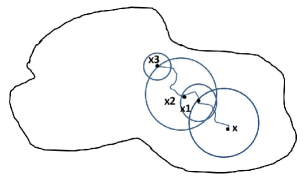
(a) WOS within the domain

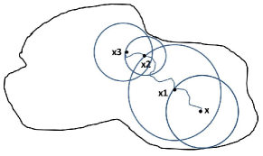
(b) WOS (with a maximal step size for each jump) within the domain

Figure 1: Walk on Spheres method

Now we can define an estimator of (3.2) with $\displaystyle c=0$ by

$$u(x)\approx\frac{1}{N}\sum_{i=1}^{N}u(x_{i}),$$ (5.7)

where $\displaystyle N$ is the number of Brownian paths sampled and $\displaystyle x_{i}$ is the first hitting point of each path on the boundary. To speed up the WOS process, maximum possible size of the sphere for each step would allow faster first hitting on the boundary.

• 
  

  WOS and RBM

For the reflecting boundary, we will construct a strip region around the boundary (see Fig. 2) and allow the process $\displaystyle X_{t}$ to move according to the law of BM continuously. Before the path enters the strip region, the radius of WOS is chosen to be of a maximum possible size less than the distance to the boundary. Once the particle is in the strip region, the radius of the WOS sphere is fixed at a constant $\displaystyle\Delta x$ (or $\displaystyle 2\Delta x$, see Fig. 3). With this approach, according to the definition (2.4), the local time may be interpreted as

$$dL(t)\approx\frac{\int_{t_{j-1}}^{t_{j}}I_{D_{\epsilon}}(X_{s})ds}{\epsilon},$$ (5.8)

which is

$$dL(t)\approx\frac{\int_{t_{j-1}}^{t_{j}}I_{D_{\epsilon}}(X_{s})ds}{\epsilon}=(n_{t_{j}}-n_{t_{j-1}})\frac{(\Delta x)^{2}}{3\epsilon},$$ (5.9)

given a prefixed constant $\displaystyle\Delta x$ in the strip region and $\displaystyle n_{t_{j}}$ be the cumulative steps that path stays within the $\displaystyle\epsilon$-region from the begining until time $\displaystyle t_{j}$ (see Remark below for definition). Notice that only those steps where the path of $\displaystyle X_{t}$ remains in the $\displaystyle\epsilon$-region will contribute to $\displaystyle n_{t_{j}}$ because the SRBM may lie out of the $\displaystyle\epsilon$-region at other steps. More details can be found in [4], where the same construction is applied for the Neumann boundary value problem. One may refer to Fig. 3 for an illustration of the behavior of path near the boundary.

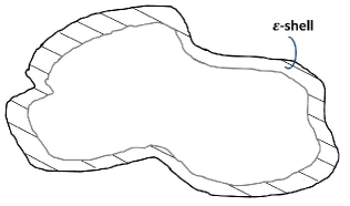
Figure 2: A $\displaystyle\epsilon$-region for a bounded domain in $\displaystyle R^{3}$

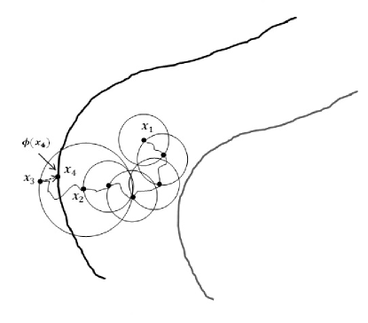
Figure 3: WOS in the $\displaystyle\epsilon$-region. At point $\displaystyle x_{1}$, BM path first hits the $\displaystyle\epsilon$-region. By WOS with a prefixed radius $\displaystyle\Delta x$, the path continues moving subsequently to $\displaystyle x_{2}$ where the distance to the boundary is less than $\displaystyle\Delta x$. Enlarge the radius to $\displaystyle 2\Delta x$, the path then have a probability to run out of the domain to $\displaystyle x_{3}$. Pull back to the closest point $\displaystyle x_{4}$ on the boundary, record $\displaystyle\phi(x_{4})$ and continue WOS-sampling starting at $\displaystyle x_{4}$.

Remark 2

Occupation time of SRBM $\displaystyle X_{t}$ in the numerator of (5.8) was calculated in terms of that of BM sampled by the walks on spheres. Notice here that within the $\displaystyle\epsilon$-region, the radius of the WOS may be $\displaystyle\Delta x$ or $\displaystyle 2\Delta x$, which implies that the corresponding elapsed time of one step for local time could be $\displaystyle(\Delta x)^{2}/3$ or $\displaystyle(2\Delta x)^{2}/3$. The latter is four times bigger than the former. But if we absorb the factor $\displaystyle 4$ into $\displaystyle n_{t}$, $\displaystyle(\ref{eq43})$ still holds. In practical implementation, we treat $\displaystyle n_{t}$ as a vector of entries of increasing value, the increment of each component of $\displaystyle n_{t}$ over the previous one after each step of WOS will be 0, 1 or 4, corresponding to the scenarios that $\displaystyle X_{t}$ is out of the $\displaystyle\epsilon$-region, in the $\displaystyle\epsilon$-region while sampled on the sphere of a radius $\displaystyle\Delta x$, or in the $\displaystyle\epsilon$-region while sampled on the sphere of a radius $\displaystyle 2\Delta x$, respectively.

Robin boundaries represent a general form of an insulating boundary condition for convection-diffusion equations where $\displaystyle c(x)$ stands for the positive diffusive coefficients. For our numerical test, we will consider two cases: a positive constant $\displaystyle c$ and a positive function $\displaystyle c(x)$.

5.2 Numerical Tests

The numerical approximations obtained are compared to the true solutions on a selected circle and a line segment, respectively, for the following three test domains in $\displaystyle R^{3}$:

1. A cube centered at the origin with a length 2;

2. A sphere centered at the origin with a radius 1;

3. An ellipsoid centered at the origin with axial lengths [3, 2, 1].

The location of the circle is given by

$$\{(x,y,z)^{T}=(r\cos\theta_{1}\sin\theta_{2},r\sin\theta_{1}\sin\theta_{2},r\cos\theta_{2})^{T}\}$$ (5.10)

with $\displaystyle r=0.6$, $\displaystyle\theta_{1}=0:k\cdot 2\pi/30:2\pi$, $\displaystyle\theta_{2}=\pi/4$ with $\displaystyle k=1,...,15$. While the line segment is defined with endpoints $\displaystyle(0.4,0.4,0.6)^{T}$ and $\displaystyle(0.1,0,0)^{T}$. Fifteen uniformly spaced points on the line are selected to monitor the accuracy of the numerical solutions.

Finally, we set the true solution of the Robin boundary problem (4.1) to be

$$u(x)=\sin 3x\sin 4y\ e^{5z}+5.$$ (5.11)

5.2.1 Constant $\displaystyle c(x)$

Example 1  $\displaystyle c(X_{t})=1$

In this case, (5.1) is reduced to

$$u(x)=E^{x}\{\int_{0}^{\infty}e^{\int_{0}^{t}dL_{t}}f(X_{t})dL_{t}\},$$ (5.12)

which is equivalent to

$$u(x)=E^{x}\{\int_{0}^{\infty}e^{L_{t}-L_{0}}f(X_{t})dL_{t}\}$$ (5.13)

or

$$u(x)=E^{x}\{\int_{0}^{\infty}e^{L_{t}}f(X_{t})dL_{t}\},$$ (5.14)

for a starting point $\displaystyle x$ belonging to the interior of the solution domain.

We will truncate the time interval to $\displaystyle[0,T]$, an approximation to (5.14) will be

$$\tilde{u}(x)=E^{x}\{\int_{0}^{T}e^{L_{t}}f(X_{t})dL_{t}\}.$$ (5.15)

Using the fact that

$$dL_{t}\approx(n_{t}-n_{t-1})\frac{(\Delta x)^{2}}{3\epsilon},$$ (5.16)

we can rewrite (5.15) as

$$\tilde{u}(x)=E^{x}\{\int_{0}^{T}e^{n_{t}\frac{(\Delta x)^{2}}{3\epsilon}}f(X_{t})(n_{t}-n_{t-1})\frac{(\Delta x)^{2}}{3\epsilon}\}.$$ (5.17)

Next identifying the time interval with the length of sample path NP, we have

$$\tilde{u}(x)=E^{x}\left\{\sum_{j^{\prime}=0}^{NP}e^{n_{t_{j}}\frac{(\Delta x)^{2}}{3\epsilon}}f(X_{t_{j}})(n_{t_{j}}-n_{t_{j-1}})\frac{(\Delta x)^{2}}{3\epsilon}\right\},$$ (5.18)

where $\displaystyle j^{\prime}$ denotes each step of the path and $\displaystyle j$ denotes the steps where the path hits the boundary.

At each step along a path we first evaluate

$$e^{n_{t_{j}}\frac{(\Delta x)^{2}}{3\epsilon}}f(X_{t_{j}})(n_{t_{j}}-n_{t_{j-1}})\frac{(\Delta x)^{2}}{3\epsilon},$$

if $\displaystyle X_{t_{j}}$ hits the boundary, we then compute $\displaystyle f(X_{t_{j}})(n_{t_{j}}-n_{t_{j-1}})\frac{(\Delta x)^{2}}{3\epsilon}$, followed by multiplying it by $\displaystyle e^{n_{t_{j}}\frac{(\Delta x)^{2}}{3\epsilon}}$, which uses the cumulative time of $\displaystyle L_{t_{j}}$ from $\displaystyle t=0$ to $\displaystyle t_{j}$. Finally, the expectation is done via the average over $\displaystyle N$ sample paths.

The simulation results of a cubic domain are presented in Fig. 4 and 5. The two figures show the convergency of the approximations as the length of path increases from $\displaystyle 1.35e4$ to $\displaystyle 1.43e4$ and $\displaystyle 1.6e4$ to $\displaystyle 1.7e4$ over the circle and the line segment, respectively. Some deviations are seen at the tail in Figure 4(a) and among the middle points in Figure 4(b). Meanwwhile, for the spherical and ellipsoid domains (Figure 6 and 7), the approximations are better and the errors are relatively smaller especially over the line segments, which are below 3% in Figure 6(b) and Figure 7(b).

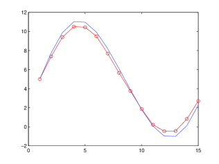
(a) $\displaystyle\epsilon$ = 3$\displaystyle\Delta x$, Err = 9.59%, NP=1.35e4, $\displaystyle\Delta x$=5e-4

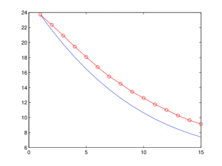
(b) $\displaystyle\epsilon$ = 4$\displaystyle\Delta x$, Err =8.84%, NP=1.6e4, $\displaystyle\Delta x$=5e-4

Figure 4: Cubic domain: number of paths $\displaystyle N=2e5$ and $\displaystyle c(X_{t})=1$. (Left - circle; right - line segement)

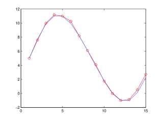
(a) $\displaystyle\epsilon$ = 3$\displaystyle\Delta x$, Err = 5.50%, NP=1.43e4, $\displaystyle\Delta x$=5e-4

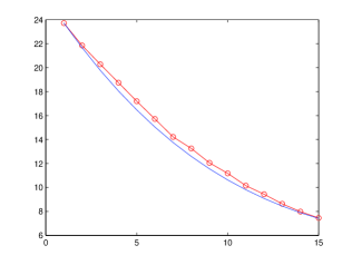
(b) $\displaystyle\epsilon$ = 4$\displaystyle\Delta x$, Err = 6.49%, NP=1.7e4, $\displaystyle\Delta x$=5e-4

Figure 5: Cubic domain: number of paths $\displaystyle N=2e5$ and $\displaystyle c(X_{t})=1$. (Left - circle; right - line segement)

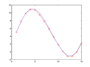
(a) $\displaystyle\epsilon$ = 3$\displaystyle\Delta x$, Err = 3.96%, NP=6e3, $\displaystyle\Delta x$=5e-4

(b) $\displaystyle\epsilon$ = 3$\displaystyle\Delta x$, Err = 1.24%, NP=5.5e3, $\displaystyle\Delta x$=5e-4

Figure 6: Spherical domain: number of paths $\displaystyle N=2e5$ and $\displaystyle c(X_{t})=1$. (Left - circle; right - line segement)

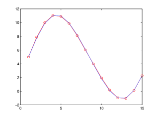
(a) $\displaystyle\epsilon$ = 3$\displaystyle\Delta x$, Err = 2.42 %, NP= 4.5e3, $\displaystyle\Delta x$=5e-4

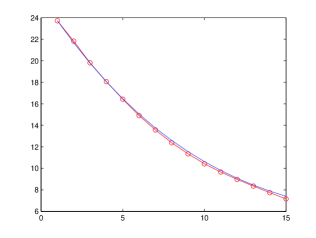
(b) $\displaystyle\epsilon$ = 3$\displaystyle\Delta x$, Err = 2.44%, NP=4.5e3, $\displaystyle\Delta x$=5e-4

Figure 7: Ellipsoid domain: number of paths $\displaystyle N=2e5$ and $\displaystyle c(X_{t})=1$. (Left - circle; right - line segement)

5.2.2 Variable c(x)

Example 2 $\displaystyle c(X_{t})=|x|$, $\displaystyle x$ is the first component of $\displaystyle X_{t}$ on the boundary. Similar to Example 1, we have

$$u(x)=E^{x}\left\{\int_{0}^{\infty}e^{\int_{0}^{t}c(X_{s})dL_{s}}f(X_{t})dL_{t}\right\}.$$ (5.19)

It can be seen that $\displaystyle c(X_{s})dL_{s}$ and $\displaystyle f(X_{t})dL_{t}$ have the same form, so we can handle $\displaystyle c(X_{s})dL_{s}$ exactly the same way as $\displaystyle f(X_{t})dL_{t}$. Then, we have

$$u(x)=E^{x}\left\{\sum_{j^{\prime}=0}^{NP}e^{\sum_{k=0}^{j}c(X_{t_{k}})(n_{t_{k}}-n_{t_{k-1}})\frac{h^{2}}{3\epsilon}}f(X_{t_{j}})(n_{t_{j}}-n_{t_{j-1}})\frac{h^{2}}{3\epsilon}\right\}.$$ (5.20)

Notice that the term

$$e^{\sum_{k=0}^{j}c(X_{t_{k}})(n_{t_{k}}-n_{t_{k-1}})\frac{h^{2}}{3\epsilon}}$$ (5.21)

cumulates all the information of $\displaystyle c(X_{t})$ with respect to the local time from the beginning to the current time. If $\displaystyle c(X_{t})=|x|$, then

$$u(x)=E^{x}\left\{\sum_{j^{\prime}=0}^{NP}e^{\sum_{k=0}^{j}|x_{t_{k}}|(n_{t_{k}}-n_{t_{k-1}})\frac{h^{2}}{3\epsilon}}f(X_{t_{j}})(n_{t_{j}}-n_{t_{j-1}})\frac{h^{2}}{3\epsilon}\right\},$$ (5.22)

where $\displaystyle j^{\prime}$ denote each step for the path and $\displaystyle j$ denotes the steps where the path hits the boundary.

Numerical results are shown in Figure 8-10 for a cubic, a spherical and an ellipsoid domain, respectively with some adjustment in $\displaystyle\Delta x$ and $\displaystyle NP$. Here we still have similar results for cube with errors around 6.5%. For the sphere, we change $\displaystyle\Delta x$ to $\displaystyle 4e-4$ and there are deviation around the middle in Figure 9(a) which may explain the overall error only 6.74% while it performs well over the line segment in Figure 9(b) with a smaller error of 3.1%. For the ellipsoid, the results are similar as in Example 1 and maintain an error below 4%.

(a) $\displaystyle\epsilon$ = 3$\displaystyle\Delta x$, Err = 6.35%, NP=1.6e4, $\displaystyle\Delta x$=5e-4

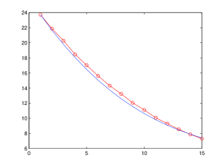
(b) $\displaystyle\epsilon$ = 3$\displaystyle\Delta x$, Err = 6.66%, NP=1.48e4, $\displaystyle\Delta x$=5e-4

Figure 8: Cubic domain: number of paths $\displaystyle N=2e5$ and $\displaystyle c(X_{t})=|x|$. (Left - circle; right - line segement)

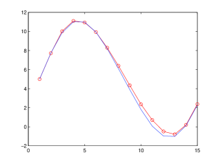
(a) $\displaystyle\epsilon$ = 3$\displaystyle\Delta x$, Err = 6.74%, NP=6.5e3, $\displaystyle\Delta x$=4e-4

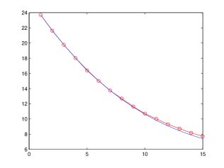
(b) $\displaystyle\epsilon$ = 3$\displaystyle\Delta x$, Err = 3.10%, NP=6e3, $\displaystyle\Delta x$=4e-4

Figure 9: Spherical domain: number of paths $\displaystyle N=2e5$ and $\displaystyle c(X_{t})=|x|$. (Left - circle; right - line segement)

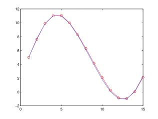
(a) $\displaystyle\epsilon$ = 3$\displaystyle\Delta x$, Err = 3.76 %, NP= 5e3, $\displaystyle\Delta x$=4e-4

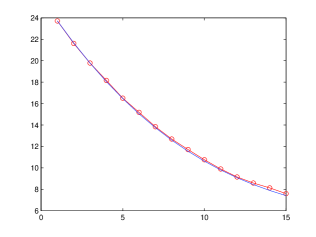
(b) $\displaystyle\epsilon$ = 3$\displaystyle\Delta x$, Err = 1.93%, NP=5e3, $\displaystyle\Delta x$=4e-4

Figure 10: Ellipsoid domain: number of paths $\displaystyle N=2e5$ and $\displaystyle c(X_{t})=|x|$. (Left - circle; right - line segement)

6 Conclusions and future work

This paper presents a Monte Carlo simulation method to solve the third boundary problems associated with Laplace equations. The idea of simulating sample paths of SRBM by the WOS within the strip region shows its efficiency and accuracy in estimating local time and evaluating Feynman-Kac formula. It should be noted that the cases that $\displaystyle q\neq 0$ needs further work due to the unknown exit time out of the sphere at each step. For the Poisson equation, the contribution of the source term might be computed as a conditional integral [19]. Moreover, the proper truncation of time period is unknown, though it is proven that the variance of the approximation increases linearly of $\displaystyle T$ [13].

For future work, more flexible domains with local convexity will be considered as it relates to the calculations of electrical properties such as the conductivity of composite materials where the particle shapes plays an important role [21].

References

- [1] A.V. Skorokhod, Stochastic equations for diffusion processes in a bounded region, Theory of Probability & Its Applications 6.3 (1961), 264-274.
- [2] V.G. Papanicolaou, The probabilistic solution of the third boundary value problem for second order elliptic equations, Probab. Th. Rel. Fields 87 (1990), 27-77.
- [3] C. Yan, W. Cai and X. Zeng, A parallel method for solving Laplace equations with Dirichlet data using local boundary integral equations and random walks, SIAM J. Scientific Computing, Vol. 35, No. 4, B868- B889, 2013.
- [4] Y. Zhou, W. Cai and (Elton) P. Hsu, Local Time of Reflecting Brownian Motion and Probabilistic Representation of the Neumann Problem, Preprint, 2015.
- [5] R.P. Feynman, Space-time approach to nonrelativistic quantum mechanics, Rev. Mod. Phys. 20 (1948), 367-387.
- [6] Kac, M., On distributions of certain Wiener functionals, Trans. Am. Math. Soc. 65 (1949): 1-13.
- [7] Kac, M., On some connections between probability theory and differential and integral equations, in: Proc. 2nd Berkeley Symp. Math. Stat. and Prob. 65 (1951): 189-215.
- [8] I. Binder and M. Braverman, The rate of convergence of the walk of sphere algorithm, Geometric and Functional Analysis, Vol. 22, 558-587, 2012.
- [9] J.-P. Morillon, Numerical solutions of linear mixed boundary value problems using stochastic representations, Int. J. Numer. Meth. Engng., Vol. 40, 387-405, 1997.
- [10] J.E. Souza de Cursi, Numerical methods for linear boundary value problems based on Feynman-Kac representations, Mathematics and computers in simulation, Vol. 36, No. 1, 1-16, 1994.
- [11] A. Lejay and S. Maire, New Monte Carlo schemes for simulating diffusions in discontinuous media, Journal of computational and applied mathematics 245 (2013): 97-116.
- [12] (Elton) P. Hsu, Reflecting Brownian motion, boundary local time and the Neumann problem, Dissertation Abstracts International Part B: Science and Engineering[DISS. ABST. INT. PT. B- SCI. ENG.], Vol. 45, No. 6, 1984.
- [13] S. Maire and E. Tanré, Monte Carlo approximations of the Neumann problem, Monte Carlo Methods and Applications 19.3 (2013): 201-236.
- [14] K. K. Sabelfeld and N. A. Simonov, Random walks on boundary for solving PDEs, Walter de Gruyter, 1994.
- [15] H. Tanaka, Stochastic differential equations with reflecting boundary condition in convex regions, Hiroshima Mathematical Journal 9.1 (1979), 163-177.
- [16] P.L. Lions and A.S. Sznitman, Stochastic differential equations with reflecting boundary conditions, Communications on Pure and Applied Mathematics 37.4 (1984), 511-537.
- [17] J.F. Douglas, Integral equation approach to condensed matter relaxation, Journal of Physics: Condensed Matter 11.10A (1999), A329.
- [18] M. Freidlin, Functional Integration and Partial Differential Equations, Princeton University Press, 1985.
- [19] C.O. Hwang, M. Mascagni, and J. A. Given, A Feynman-Kac path-integral implementation for Poisson’s equation using an h-conditioned Green’s function, Mathematics and computers in simulation 62.3 (2003), 347-355.
- [20] K. L. Chung, Green, Brown, and Probability and Brownian Motion on the Line, World Scientific Pub Co Inc, 2002.
- [21] D.J. Audus, A.M. Hassan, E.J. Garboczi and J.F. Douglas, Interplay of particle shape and suspension properties: a study of cube-like particles, Soft matter 11.17 (2015), 3360-3366.
- [22] B. Øksendal, Stochastic differential equations, Springer Berlin Heidelberg, 2003.
- [23] I. Karatzas and S. E. Shreve, Brownian motion and stochastic calculus, Springer-Verlag New York Inc., 1988.
- [24] M.E. Müller, Some continuous Monte Carlo methods for the Dirichlet problem, The Annals of Mathematical Statistics, Vol. 27, No. 3, 569-589, 1956.
- [25] K. Burdzy, Z. Chen and J. Sylvester, The heat equation and reflected Brownian motion in time-dependent domains, The Annuals of Probability 32. 1B (2004), 775-804.