On the Asymptotic Efficiency of Approximate Bayesian Computation Estimators

Abstract

Many statistical applications involve models for which it is difficult to evaluate the likelihood, but from which it is relatively easy to sample. Approximate Bayesian computation is a likelihood-free method for implementing Bayesian inference in such cases. We present results on the asymptotic variance of estimators obtained using approximate Bayesian computation in a large-data limit. Our key assumption is that the data are summarized by a fixed-dimensional summary statistic that obeys a central limit theorem. We prove asymptotic normality of the mean of the approximate Bayesian computation posterior. This result also shows that, in terms of asymptotic variance, we should use a summary statistic that is the same dimension as the parameter vector, $p$; and that any summary statistic of higher dimension can be reduced, through a linear transformation, to dimension $p$ in a way that can only reduce the asymptotic variance of the posterior mean. We look at how the Monte Carlo error of an importance sampling algorithm that samples from the approximate Bayesian computation posterior affects the accuracy of estimators. We give conditions on the importance sampling proposal distribution such that the variance of the estimator will be the same order as that of the maximum likelihood estimator based on the summary statistics used. This suggests an iterative importance sampling algorithm, which we evaluate empirically on a stochastic volatility model.

1 Introduction

Many statistical applications involve inference about models that are easy to simulate from, but for which it is difficult, or impossible, to calculate likelihoods. In such situations it is possible to use the fact we can simulate from the model to enable us to perform inference. There is a wide class of such likelihood-free methods of inference including indirect inference Gouriéroux & Ronchetti (1993); Heggland & Frigessi (2004), the bootstrap filter Gordon et al. (1993), simulated methods of moments Duffie & Singleton (1993), and synthetic likelihood Wood (2010).

We consider a Bayesian version of these methods, termed approximate Bayesian computation. This involves defining an approximation to the posterior distribution in such a way that it is possible to sample from this approximate posterior using only the ability to sample from the model. Arguably the first approximate Bayesian computation method was that of Pritchard et al. (1999), and these methods have been popular within population genetics Beaumont et al. (2002), ecology Beaumont (2010) and systems biology Toni et al. (2009). More recently, there have been applications to areas including stereology Bortot et al. (2007), finance Peters et al. (2011) and cosmology Ishida et al. (2015).

Let $K({}{x})$ be a density kernel, scaled, without loss of generality, so that $\max_{{}{x}}K({}{x})=1$. Further, let $\varepsilon>0$ be a bandwidth. Denote the data by ${}{Y}_{\rm obs}=(y_{\rm obs,1},\ldots,y_{\rm obs,n})$. Assume we have chosen a finite-dimensional summary statistic ${}{s}_{n}({}{Y})$, and denote ${}{s}_{\rm obs}={}{s}_{n}({}{Y}_{\rm obs})$. If we model the data as a draw from a parametric density, $f_{n}({}{y}\mid{}{\theta})$, and assume prior, $\pi({}{\theta})$, then we define the approximate Bayesian computation posterior as

$$\pi_{\rm ABC}({}{\theta}\mid{}{s}_{\rm obs},\varepsilon)\propto\pi({}{\theta})\int f_{n}({}{s}_{\rm obs}+\varepsilon{}{v}\mid{}{\theta})K({}{v})\,d{}{v},$$ (1)

where $f_{n}({}{s}\mid{}{\theta})$ is the density for the summary statistic implied by $f_{n}({}{y}\mid{}{\theta})$. Let $f_{\rm ABC}({}{s}_{\rm obs}\mid{}{\theta},\varepsilon)=\int f_{n}({}{s}_{\rm obs}+\varepsilon{}{v}\mid{}{\theta})K({}{v})\,d{}{v}$. This framework encompasses most implementations of approximate Bayesian computation. In particular, the use of the uniform kernel corresponds to the popular rejection-based rule Beaumont et al. (2002).

The idea is that $f_{\rm ABC}({}{s}_{\rm obs}\mid{}{\theta},\varepsilon)$ is an approximation of the likelihood. The approximate Bayesian computation posterior, which is proportional to the prior multiplied by this likelihood approximation, is an approximation of the true posterior. The likelihood approximation can be interpreted as a measure of how close, on average, the summary, ${}{s}_{n}$, simulated from the model is to the summary for the observed data, ${}{s}_{\rm obs}$. The choices of kernel and bandwidth determine the definition of closeness.

By defining the approximate posterior in this way, we can simulate samples from it using standard Monte Carlo methods. One approach, that we will focus on later, uses importance sampling. Let $K_{\varepsilon}({}{x})=K({}{x}/\varepsilon)$. Given a proposal density, $q_{n}({}{\theta})$, a bandwidth, $\varepsilon$, and a Monte Carlo sample size, $N$, an importance sampler would proceed as in Algorithm 1. The set of accepted parameters and their associated weights provides a Monte Carlo approximation to $\pi_{\rm ABC}$. If we set $q_{n}({}{\theta})=\pi({}{\theta})$ then this is just a rejection sampler. In practice sequential importance sampling methods are often used to learn a good proposal distribution Beaumont et al. (2009).

Importance and rejection sampling approximate Bayesian computation

1. Simulate ${}{\theta}_{1},\ldots,{}{\theta}_{N}\sim q_{n}({}{\theta})$;

2. For each $i=1,\ldots,N$, simulate ${}{Y}^{(i)}=\{y_{1}^{(i)},\ldots,y_{n}^{(i)}\}\sim f_{n}(y\mid{}{\theta}_{i})$;

3. For each $i=1,\ldots,N$, accept ${}{\theta}_{i}$ with probability $K_{\varepsilon}\{{}{s}_{n}^{(i)}-{}{s}_{\rm obs}\}$, where ${}{s}_{n}^{(i)}={}{s}_{n}\{{}{Y}^{(i)}\}$;

and define the associated weight as $w_{i}=\pi({}{\theta}_{i})/q_{n}({}{\theta}_{i})$.

There are three choices in implementing approximate Bayesian computation: the choice of summary statistic, the choice of bandwidth, and the Monte Carlo algorithm. For importance sampling, the last of these involves specifying the Monte Carlo sample size, $N$, and the proposal density, $q_{n}({}{\theta})$. These, roughly, relate to three sources of approximation. To see this, note that as $\varepsilon\rightarrow 0$ we would expect (1) to converge to the posterior given ${}{s}_{\rm obs}$ Fearnhead & Prangle (2012). Thus the choice of summary statistic governs the approximation, or loss of information, between using the full posterior distribution and using the posterior given the summary. The value $\varepsilon$ then affects how close the approximate Bayesian computation posterior is to the posterior given the summary. Finally there is Monte Carlo error from approximating the approximate Bayesian computation posterior with a Monte Carlo sample. The Monte Carlo error is not only affected by the Monte Carlo algorithm, but also by the choices of summary statistic and bandwidth, which together affect the probability of acceptance in step 3 of Algorithm 1. Having a higher-dimensional summary statistic, or a smaller value of $\varepsilon$, will tend to reduce this acceptance probability and hence increase the Monte Carlo error.

This work studies the interaction between the three sources of error, when the summary statistics obey a central limit theorem for large $n$. We are interested in the efficiency of approximate Baysian computation, where by efficiency we mean that an estimator obtained from running Algorithm 1 has the same rate of convergence as the maximum likelihood estimator for the parameter given the summary statistic. In particular, this work is motivated by the question of whether approximate Bayesian computation can be efficient as $n\rightarrow\infty$ if we have a fixed Monte Carlo sample size. Intuitively this appears unlikely. For efficiency we will need $\varepsilon\rightarrow 0$ as $n\rightarrow\infty$, and this corresponds to an increasingly strict condition for acceptance. Thus we may imagine that the acceptance probability will necessarily tend to zero as $n$ increases, and we will need an increasing Monte Carlo sample size to compensate for this.

However our results show that Algorithm 1 can be efficient if we choose proposal distribution, with a suitable scale and location and appropriately heavy tails. If we use such a proposal distribution and have a summary statistic of the same dimension as the parameter vector, then the posterior mean of approximate Bayesian computation is asymptotically unbiased with a variance that is $1+O(1/N)$ times that of the estimator maximising the likelihood of the summary statistic. This is similar to asymptotic results for indirect inference Gouriéroux & Ronchetti (1993); Heggland & Frigessi (2004). Our results also lend theoretical support to methods that choose the bandwidth indirectly by specifying the proportion of samples that are accepted, as this leads to a bandwidth which is of the optimal order in $n$.

We first prove a Bernstein-von Mises type theorem for the posterior mean of approximate Bayesian computation. This is a non-standard convergence result, as it is based on the partial information contained in the summary statistics. For related convergence results see Clarke & Ghosh (1995) and Yuan & Clarke (2004), though these do not consider the case when the dimension of the summary statistic is larger than that of the parameter. Dealing with this case introduces extra challenges.

Our convergence result for the posterior mean of approximate Bayesian computation has practically important consequences. It shows that any $d$-dimensional summary with $d>p$ can be projected to a $p$-dimensional summary statistic without any loss of information. Furthermore it shows that using a summary statistic of dimension $d>p$ can lead to an increased bias, so the asymptotic variance can be reduced if the optimal $p$-dimensional projected summary is used instead. If a $d$-dimensional summary is used, with $d>p$, it suggests choosing the variance of the kernel to match the variance of the summary statistics.

This paper adds to a growing literature on the theoretical properties of approximate Bayesian computation. Initial results focussed on comparing the bias of approximate Bayesian computation to the Monte Carlo error, and how these depend on the choice of $\varepsilon$. The convergence rate of the bias is shown to be $O(\varepsilon^{2})$ in various settings (e.g., Barber et al., 2015). This can then be used to consider how the choice of $\varepsilon$ should depend on the Monte Carlo sample size so as to balance bias and Monte Carlo variability Blum (2010); Barber et al. (2015); Biau et al. (2015). There has also been work on consistency of approximate Bayesian computation estimators. Marin et al. (2014) consider consistency when performing model choice and Frazier et al. (2016) consider consistency for parameter estimation. The latter work, which appeared after the first version of this paper, includes a result on the asymptotic normality of the posterior mean similar to our Theorem 3.1, albeit under different conditions, and also gives results on the asymptotic form of the posterior obtained using approximate Bayesian computation. This shows that for many implementations of approximate Bayesian computation, the posterior will over-estimate the uncertainty in the parameter estimate that it gives.

Finally, a number of papers have looked at the choice of summary statistics (e.g., Wegmann et al., 2009; Blum, 2010; Prangle et al., 2014). Our Theorem 3.1 gives insight into this. As mentioned above, this result shows that, in terms of minimising the asymptotic variance, we should use a summary statistic of the same dimension as the number of parameters. In particular it supports the suggestion in Fearnhead & Prangle (2012) of having one summary per parameter, with that summary approximating the maximum likelihood estimator for that parameter.

2 Notation and Set-up

Denote the data by ${}{Y}_{\rm obs}=(y_{{\rm obs},1},\ldots,$ $y_{{\rm obs},n})$, where $n$ is the sample size, and each observation, $y_{{\rm obs},i}$, can be of arbitrary dimension. We make no assumption directly on the data, but make assumptions on the distribution of the summary statistics. We consider the asymptotics as $n\rightarrow\infty$, and denote the density of ${}{Y}_{\rm obs}$ by $f_{n}({}{y}\mid{}{\theta})$, where ${}{\theta}\in\mathcal{P}\subset\mathbb{R}^{p}$. We let ${}{\theta}_{0}$ denote the true parameter value, and $\pi({}{\theta})$ its prior distribution. For a set $A$, let $A^{c}$ be its complement with respect to the whole space.

We assume that ${}{\theta}_{0}$ is in the interior of the parameter space, and that the prior is differentiable in a neighbourhood of the true parameter: There exists some $\delta_{0}>0$, such that $\mathcal{P}_{0}=\{{}{\theta}:|{}{\theta}-{}{\theta}_{0}|<\delta_{0}\}\subset\mathcal{P}$, $\pi({}{\theta})\in C^{1}(\mathcal{P}_{0})$ and $\pi({}{\theta}_{0})>0$.

To implement approximate Bayesian computation we will use a $d$-dimensional summary statistic, ${}{s}_{n}({}{Y})\in\mathbb{R}^{d}$; such as a vector of sample means of appropriately chosen functions. We assume that ${}{s}_{n}({}{Y})$ has a density function, which depends on $n$, and we denote this by $f_{n}({}{s}\mid{}{\theta})$. We will use the shorthand ${}{S}_{n}$ to denote the random variable with density $f_{n}({}{s}\mid{}{\theta})$. In approximate Bayesian computation we use a kernel, $K({}{x})$, with $\max_{{}{x}}K({}{x})=1$, and a bandwidth $\varepsilon>0$. As we vary $n$ we will often wish to vary $\varepsilon$, and in these situations we denote the bandwidth by $\varepsilon_{n}$. For Algorithm 1 we require a proposal distribution, $q_{n}({}{\theta})$, and allow this to depend on $n$. We assume the following conditions on the kernel, which are satisfied by all commonly-used kernels, The kernel satisfies (i) $\int{}{v}K({}{v})\,d{}{v}=0$; (ii) $\int\prod_{k=1}^{l}v_{i_{k}}K({}{v})\,d{}{v}<\infty$ for any coordinates $(v_{i_{1}},\ldots,v_{i_{l}})$ of ${}{v}$ and $l\leq p+6$; (iii) $K({}{v})\propto\overline{K}(\|{}{v}\|_{\Lambda}^{2})$ where $\|{}{v}\|_{\Lambda}^{2}={}{v}^{T}\Lambda{}{v}$ and $\Lambda$ is a positive-definite matrix, and $K({}{v})$ is a decreasing function of $\|{}{v}\|_{\Lambda}$; (iv) $K({}{v})=O(e^{-c_{1}\|{}{v}\|_{\Lambda}^{\alpha_{1}}})$ for some $\alpha_{1}>0$ and $c_{1}>0$ as $\|{}{v}\|_{\Lambda}\rightarrow\infty$.

For a real function $g({}{x})$ denote its $k$th partial derivative at ${}{x}={}{x}_{0}$ by $D_{x_{k}}g({}{x}_{0})$, the gradient function by $D_{{}{x}}g({}{x}_{0})$ and the Hessian matrix by $H_{{}{x}}g({}{x}_{0})$. To simplify notation, $D_{\theta_{k}}$, $D_{{}{\theta}}$ and $H_{{}{\theta}}$ are written as $D_{k}$, $D$ and $H$ respectively. For a series $x_{n}$ we use the notation that for large enough $n$, $x_{n}=\Theta(a_{n})$ if there exist constants $m$ and $M$ such that $0<m<|x_{n}/a_{n}|<M<\infty$, and $x_{n}=\Omega(a_{n})$ if $|x_{n}/a_{n}|\rightarrow\infty$. For two square matrices $A$ and $B$, we say $A\leq B$ if $B-A$ is semi-positive definite, and $A<B$ if $B-A$ is positive definite.

Our theory will focus on estimates of some function, ${}{h}(\theta)$, of $\theta$, which satisfies differentiability and moment conditions that will control the remainder terms in a Taylor-expansions. The $k$th coordinate of ${}{h}({}{\theta})$, $h_{k}({}{\theta})$, satisfies (i) $h_{k}({}{\theta})\in C^{1}(\mathcal{P}_{0})$; (ii) $D_{k}h({}{\theta}_{0})\neq 0$; and (iii) $\int h_{k}({}{\theta})^{2}\pi({}{\theta})\,d{}{\theta}<\infty$.

The asymptotic results presuppose a central limit theorem for the summary statistic. There exists a sequence $a_{n}$, with $a_{n}\rightarrow\infty$ as $n\rightarrow\infty$, a $d$-dimensional vector ${}{s}({}{\theta})$ and a $d\times d$ matrix $A({}{\theta})$, such that for all ${}{\theta}\in\mathcal{P}_{0}$,

$$a_{n}\{{}{S}_{n}-{}{s}({}{\theta})\}\rightarrow N\{0,A({}{\theta})\},~{}~{}\mbox{$n\rightarrow\infty$},$$

with convergence in distribution. We also assume that $s_{\rm obs}\rightarrow s(\theta_{0})$ in probability. Furthermore, (i) ${}{s}({}{\theta})\in C^{1}(\mathcal{P}_{0})$ and $A({}{\theta})\in C^{1}(\mathcal{P}_{0})$, and $A({}{\theta})$ is positive definite for ${}{\theta}\in\mathcal{P}_{0}$; (ii) for any $\delta>0$ there exists a $\delta^{\prime}>0$ such that $\|s(\theta)-s(\theta_{0})\|>\delta^{\prime}$ for all $\theta$ satisfying $\|\theta-\theta_{0}\|>\delta$; (iii) $I({}{\theta})=D{}{s}({}{\theta})^{T}A^{-1}({}{\theta})D{}{s}({}{\theta})$ has full rank at ${}{\theta}={}{\theta}_{0}$.

Under Condition 2, $a_{n}$ is the rate of convergence in the central limit theorem. If the data are independent and identically distributed, and the summaries are sample means of functions of the data or of quantiles, then $a_{n}=n^{1/2}$. In most applications the data will be dependent, but if summaries are sample means Wood (2010), quantiles Peters et al. (2011); Allingham et al. (2009); Blum & François (2010) or linear combinations thereof Fearnhead & Prangle (2012) then a central limit theorem will often still hold, though $a_{n}$ may increase more slowly than $n^{1/2}$.

Part (ii) of Condition 2 is required for the true parameter to be identifiable given only the summary of data. The asymptotic variance of the summary-based maximum likelihood estimator for ${}{\theta}$ is $I^{-1}({}{\theta}_{0})/a_{n}^{2}$. Condition (iii) ensures that this variance is valid at the true parameter.

We next require a condition that controls the difference between $f_{n}({}{s}\mid{}{\theta})$ and its limiting distribution for ${}{\theta}\in\mathcal{P}_{0}$. Let $N({}{x};{}{\mu},\Sigma)$ be the normal density at ${}{x}$ with mean ${}{\mu}$ and variance $\Sigma$. Define $\widetilde{f}_{n}({}{s}\mid{}{\theta})=N\{{}{s};{}{s}({}{\theta}),A({}{\theta})/a_{n}^{2}\}$ and the standardized random variable $W_{n}({}{s})=a_{n}A({}{\theta})^{-1/2}\{{}{s}-{}{s}({}{\theta})\}$. Let $\widetilde{f}_{W_{n}}({}{w}\mid{}{\theta})$ and $f_{W_{n}}({}{w}\mid{}{\theta})$ be the density of $W_{n}({}{s})$ when ${}{s}\sim\widetilde{f}_{n}({}{s}\mid{}{\theta})$ and $f_{n}({}{s}\mid{}{\theta})$ respectively. The condition below requires that the difference between $f_{W_{n}}({}{w}\mid{}{\theta})$ and its Edgeworth expansion $\widetilde{f}_{W_{n}}({}{w}\mid{}{\theta})$ is $o(a_{n}^{-2/5})$ and can be bounded by a density with exponentially decreasing tails. This is weaker than the standard requirement, $o(a_{n}^{-1})$, for the remainder in the Edgeworth expansion.

There exists $\alpha_{n}$ satisfying $\alpha_{n}/a_{n}^{2/5}\rightarrow\infty$ and a density $r_{\rm max}({}{w})$ satisfying Condition 2 (ii)-(iii) where $K({}{v})$ is replaced with $r_{\rm max}({}{w})$, such that $\sup_{{}{\theta}\in\mathcal{P}_{0}}\alpha_{n}|f_{W_{n}}({}{w}\mid{}{\theta})-\widetilde{f}_{W_{n}}({}{w}\mid{}{\theta})|\leq c_{3}r_{\rm max}({}{w})$ for some positive constant $c_{3}$.

The following condition further assumes that $f_{n}(s\mid\theta)$ has exponentially decreasing tails with rate uniform in the support of $\pi(\theta)$.

The following statements hold: (i) $r_{\rm max}(w)$ satisfies Condition 2 (iv); and (ii) $\sup_{\theta\in\mathcal{P}_{0}^{c}}f_{W_{n}}(w\mid\theta)=O(e^{-c_{2}\|w\|^{\alpha_{2}}})$ as $\|w\|\rightarrow\infty$ for some positive constants $c_{2}$ and $\alpha_{2}$, and $A(\theta)$ is bounded in $\mathcal{P}$.

3 Posterior mean asymptotics

We first ignore any Monte Carlo error, and focus on the ideal estimator of true posterior mean from approximate Bayesian computation. This is the posterior mean, ${}{h}_{\rm ABC}$, where

$${}{h}_{\rm ABC}={E}_{\pi_{\rm ABC}}\{{}{h}({}{\theta})\mid{}{s}_{\rm obs}\}=\int{}{h}({}{\theta})\pi_{\rm ABC}({}{\theta}\mid{}{s}_{\rm obs},\varepsilon_{n}).$$

This estimator depends on $\varepsilon_{n}$, but we suppress this from the notation. As an approximation to the true posterior mean, ${E}\{{}{h}({}{\theta})\mid{}{Y}_{\rm obs}\}$, ${}{h}_{\rm ABC}$ contains errors from the choice of the bandwidth $\varepsilon_{n}$ and summary statistic ${}{s}_{\rm obs}$.

To understand the effect of these two sources of error, we derive results for the asymptotic distributions of ${}{h}_{\rm ABC}$ and the likelihood-based estimators, including the summary-based maximum likelihood estimator and the summary-based posterior mean, where we consider randomness solely due to the randomness of the data. Let $T_{{\rm obs}}=a_{n}A(\theta_{0})^{-1/2}\{s_{\rm obs}-s(\theta_{0})\}$.

Theorem 3.1.

Assume Conditions 2–2.

• Let $\hat{{{}{\theta}}}_{{}_{\mbox{\scriptsize\rm MLES}}}=\mbox{argmax}_{{}{\theta}\in\mathcal{P}}\log f_{n}({}{s}_{\rm obs}\mid{}{\theta})$. For ${}{h}_{{}{s}}={}{h}(\hat{{{}{\theta}}}_{{}_{\mbox{\scriptsize\rm MLES}}})$ or ${E}\{{}{h}({}{\theta})\mid{}{s}_{\rm obs}\}$,

  $$a_{n}\{{}{h}_{{}{s}}-{}{h}({}{\theta}_{0})\}\rightarrow N\{0,D{}{h}({}{\theta}_{0})^{T}I^{-1}({}{\theta}_{0})D{}{h}({}{\theta}_{0})\},~{}~{}n\rightarrow\infty,$$

  with convergence in distribution.

• Define $c_{\infty}=\lim_{n\rightarrow\infty}a_{n}\varepsilon_{n}$. Let $Z$ be the weak limit of $T_{\rm obs}$, which has a standard normal distribution, and $R(c_{\infty},Z)$ be a random vector with mean zero that is defined in the Supplementary Material. If $\varepsilon_{n}=o(a_{n}^{-3/5})$, then

  $$a_{n}\{h_{{\rm ABC}}-h(\theta_{0})\}\rightarrow Dh(\theta_{0})^{T}\{I(\theta_{0})^{-1/2}Z+R(c_{\infty},Z)\},~{}~{}n\rightarrow\infty,$$

  with convergence in distribution. If either (i) $\varepsilon_{n}=o(a_{n}^{-1})$; (ii) $d=p$; or (iii) the covariance matrix of $K(v)$ is proportional to $A(\theta_{0})$; then $R(c_{\infty},Z)=0$. For other cases, the variance of $I(\theta_{0})^{-1/2}Z+R(c_{\infty},Z)$ is no less than $I^{-1}(\theta_{0})$.

Theorem 3.1 (i) shows the validity of posterior inference based on the summary statistics. Regardless of the sufficiency and dimension of ${}{s}_{\rm obs}$, the posterior mean based on the summary statistics is consistent and asymptotically normal with the same variance as the summary-based maximum likelihood estimator.

Denote the bias of approximate Bayesian computation, ${}{h}_{\rm ABC}-{E}\{{}{h}({}{\theta})\mid{}{s}_{\rm obs}\}$, by $\mbox{bias}_{\rm ABC}$. The choice of bandwidth impacts the size of the bias. Theorem 3.1 (ii) indicates two regimes for the bandwidth for which the posterior mean of approximate Bayesian computation has good properties.

The first case is when $\varepsilon_{n}$ is $o(1/a_{n})$. For this regime the posterior mean of approximate Bayesian computation always has the same asymptotic distribution as that of the true posterior given the summaries. The other case is when $\varepsilon_{n}$ is $o(a_{n}^{-3/5})$ but not $o(n^{-1})$. We obtain the same asymptotic distribution if either $d=p$ or we choose the kernel variance to be proportional to the variance of the summary statistics. In general for this regime of $\varepsilon_{n}$, ${}{h}_{\rm ABC}$ will be less efficient than the summary-based maximum likelihood estimator.

When $d>p$, Theorem 3.1 (ii) shows that $\mbox{bias}_{\rm ABC}$ is non-negligible and can increase the asymptotic variance. This is because the leading term of $\mbox{bias}_{\rm ABC}$ is proportional to the average of ${}{v}={}{s}-{}{s}_{\rm obs}$, the difference between the simulated and observed summary statistics. If $d>p$, the marginal density of ${}{v}$ is generally asymmetric, and thus is no longer guaranteed to have a mean of zero. One way to ensure that there is no increase in the asymptotic variance is to choose the variance of the kernel to be proportional to the variance of the summary statistics.

The loss of efficiency we observe in Theorem 3.1 (ii) for $d>p$ gives an advantage for choosing a summary statistic with $d=p$. The following proposition shows that for any summary statistic of dimension $d>p$ we can find a new $p$-dimensional summary statistic without any loss of information. The proof of the proposition is trivial and hence omitted.

Proposition 3.2.

Assume the conditions of Theorem 3.1. If $d>p$, define $C=D{}{s}({}{\theta}_{0})^{T}A({}{\theta}_{0})^{-1}$. The $p$-dimensional summary statistic $C{}{S}_{n}$ has the same information matrix, $I({}{\theta})$, as ${}{S}_{n}$. Therefore the asymptotic variance of ${}{h}_{\rm ABC}$ based on $C{}{s}_{\rm obs}$ is smaller than or equal to that based on ${}{s}_{\rm obs}$.

Theorem 3.1 leads to following natural definition.

Definition 3.3.

Assume that the conditions of Theorem 3.1 hold. Then the asymptotic variance of ${}{h}_{\rm ABC}$ is

$$\textsc{AV}_{{}{h}_{\rm ABC}}=\frac{1}{a_{n}^{2}}D{}{h}({}{\theta}_{0})^{T}I_{\rm ABC}^{-1}({}{\theta}_{0})D{}{h}({}{\theta}_{0}).$$

4 Asymptotic Properties of Rejection and Importance Sampling Algorithm

4.1 Asymptotic Monte Carlo Error

We now consider the Monte Carlo error involved in estimating ${}{h}_{\rm ABC}$. Here we fix the data and consider solely the stochasticity of the Monte Carlo algorithm. We focus on Algorithm 1. Remember that $N$ is the Monte Carlo sample size. For $i=1,\ldots,N$, ${}{\theta}_{i}$ is the proposed parameter value and $w_{i}$ is its importance sampling weight. Let $\phi_{i}$ be the indicator that is 1 if and only if $\theta_{i}$ is accepted in step 3 of Algorithm 1 and let $N_{\rm acc}=\sum_{i=1}^{N}\phi_{i}$ be the number of accepted parameter.

Provided $N_{\rm acc}\geq 1$ we can estimate ${}{h}_{\rm ABC}$ from the output of Algorithm 1 with

$$\widehat{{}{h}}=\sum_{i=1}^{N}{}{h}({}{\theta}_{i})w_{i}\phi_{i}\Big{/}\sum_{i=1}^{N}w_{i}\phi_{i}.$$

Define the acceptance probability

$$p_{{\rm acc},q}=\int q({}{\theta})\int f_{n}({}{s}\mid{}{\theta})K_{\varepsilon}({}{s}-{}{s}_{\rm obs})\mbox{d}{}{s}\mbox{d}{}{\theta},$$

and the density of the accepted parameter

$$q_{\rm ABC}({}{\theta}\mid{}{s}_{\rm obs},\varepsilon)=\frac{q_{n}({}{\theta})f_{\rm ABC}({}{s}_{\rm obs}\mid{}{\theta},\varepsilon)}{\int q_{n}({}{\theta})f_{\rm ABC}({}{s}_{\rm obs}\mid{}{\theta},\varepsilon)\,d\theta}.$$

Finally, define

$$\Sigma_{{\rm IS},n}=E_{\pi_{\rm ABC}}\left\{({}{h}({}{\theta})-{}{h}_{\rm ABC})^{2}\frac{\pi_{\rm ABC}({}{\theta}\mid{}{s}_{\rm obs},\varepsilon_{n})}{q_{\rm ABC}({}{\theta}\mid{}{s}_{\rm obs},\varepsilon_{n})}\right\},$$

$$\Sigma_{{\rm ABC},n}=p_{{\rm acc},q_{n}}^{-1}\Sigma_{{\rm IS},n},$$ (2)

where $\Sigma_{{\rm IS},n}$ is the importance sampling variance with $\pi_{\rm ABC}$ as the target density and $q_{\rm ABC}$ as the proposal density. Note that $p_{{\rm acc},q_{n}}$ and $\Sigma_{{\rm IS},n}$, and hence $\Sigma_{{\rm ABC},n}$, depend on ${}{s}_{\rm obs}$.

Standard results give the following asymptotic distribution of $\widehat{{}{h}}$.

Proposition 4.1.

For a given $n$ and ${}{s}_{\rm obs}$, if ${}{h}_{\rm ABC}$ and $\Sigma_{{\rm ABC},n}$ are finite, then

$${N}^{1/2}(\widehat{{}{h}}-{}{h}_{\rm ABC})\rightarrow N(0,\Sigma_{{\rm ABC},n}),$$

in distribution as $N\rightarrow\infty$.

This proposition motivates the following definition.

Definition 4.2.

For a given $n$ and ${}{s}_{\rm obs}$, assume that the conditions of Proposition 4.1 hold. Then the asymptotic Monte Carlo variance of $\widehat{{}{h}}$ is

$$\textsc{MCV}_{\widehat{{}{h}}}=\frac{1}{N}\Sigma_{{\rm ABC},n}.$$

4.2 Asymptotic efficiency

We have defined the asymptotic variance as $n\rightarrow\infty$ of ${}{h}_{\rm ABC}$, and the asymptotic Monte Carlo variance, as $N\rightarrow\infty$ of $\widehat{{}{h}}$. The error of ${}{h}_{\rm ABC}$ when estimating ${}{h}({}{\theta}_{0})$ and the Monte Carlo error of $\widehat{{}{h}}$ when estimating ${}{h}_{\rm ABC}$ are independent, which suggests the following definition.

Definition 4.3.

Assume the conditions of Theorem 3.1, and that ${}{h}_{\rm ABC}$ and $\Sigma_{{\rm ABC},n}$ are bounded in probability for any $n$. Then the asymptotic variance of $\widehat{{}{h}}$ is

$$\textsc{AV}_{\widehat{{}{h}}}=\frac{1}{a_{n}^{2}}{}{h}({}{\theta}_{0})^{T}I_{\rm ABC}^{-1}({}{\theta}_{0})D{}{h}({}{\theta}_{0})+\frac{1}{N}\Sigma_{{\rm ABC},n}.$$

We can interpret the asymptotic variance of $\widehat{{}{h}}$ as a first-order approximation to the variance of our Monte Carlo estimator for both large $n$ and $N$. We wish to investigate the properties of this asymptotic variance, for large but fixed $N$, as $n\rightarrow\infty$. The asymptotic variance itself depends on $n$, and we would hope it would tend to zero as $n$ increases. Thus we will study the ratio of $\textsc{AV}_{\widehat{{}{h}}}$ to $\textsc{AV}_{\mbox{\scriptsize\rm MLES}}$, where, by Theorem 3.1, the latter is $a_{n}^{-2}{}{h}({}{\theta}_{0})^{T}I^{-1}({}{\theta}_{0})D{}{h}({}{\theta}_{0})$. This ratio measures the efficiency of our Monte Carlo estimator relative to the maximum likelihood estimator based on the summaries; it quantifies the loss of efficiency from using a non-zero bandwidth and a finite Monte Carlo sample size.

We will consider how this ratio depends on the choice of $\varepsilon_{n}$ and $q_{n}({}{\theta})$. Thus we introduce the following definition:

Definition 4.4.

For a choice of $\varepsilon_{n}$ and $q_{n}({}{\theta})$, we define the asymptotic efficiency of $\widehat{{}{h}}$ as

$$\textsc{AE}_{\widehat{{}{h}}}=\lim_{n\rightarrow\infty}\frac{\textsc{AV}_{\mbox{\scriptsize\rm MLES}}}{\textsc{AV}_{\widehat{{}{h}}}}.$$

If this limiting value is zero, we say that $\widehat{{}{h}}$ is asymptotically inefficient.

We will investigate the asymptotic efficiency of $\widehat{{}{h}}$ under the assumption of Theorem 3.1 that $\varepsilon_{n}=o(a_{n}^{-3/5})$. We shall see that the convergence rate of the importance sampling variance $\Sigma_{{\rm IS},n}$ depends on how large $\varepsilon_{n}$ is relative to $a_{n}$, and so we further define $a_{n,\varepsilon}=a_{n}$ if $\lim_{n\rightarrow\infty}a_{n}\varepsilon_{n}<\infty$ and $a_{n,\varepsilon}=\varepsilon_{n}^{-1}$ otherwise.

If our proposal distribution in Algorithm 1 is either the prior or the posterior, then the estimator is asymptotically inefficient.

Theorem 4.5.

Assume the conditions of Theorem 3.1.

• If $q_{n}({}{\theta})=\pi({}{\theta})$, then $p_{{\rm acc},q_{n}}=\Theta_{p}(\varepsilon_{n}^{d}a_{n,\varepsilon}^{d-p})$ and $\Sigma_{{\rm IS},n}=\Theta_{p}(a_{n,\varepsilon}^{-2})$.

• If $q_{n}({}{\theta})=\pi_{\rm ABC}({}{\theta}\mid{}{s}_{\rm obs},\varepsilon_{n})$, then $p_{{\rm acc},q_{n}}=\Theta_{p}(\varepsilon_{n}^{d}a_{n,\varepsilon}^{d})$ and $\Sigma_{{\rm IS},n}=\Theta_{p}(a_{n,\varepsilon}^{p})$.

In both cases $\widehat{{}{h}}$ is asymptotically inefficient.

The result in part (ii) shows a difference from standard importance sampling settings, where using the target distribution as the proposal leads to an estimator with no Monte Carlo error.

The estimator $\widehat{{}{h}}$ is asymptotically inefficient because the Monte Carlo variance decays more slowly than $1/a_{n}^{2}$ as $n\rightarrow\infty$. However this is caused by different factors in each case.

To see this, consider the acceptance probability of a value of $\theta$ and corresponding summary ${}{s}_{n}$ simulated in one iteration of Algorithm 1. This acceptance probability depends on

$$\frac{{}{s}_{n}-{}{s}_{\rm obs}}{\varepsilon_{n}}=\frac{1}{\varepsilon_{n}}\left[\{{}{s}_{n}-{}{s}({}{\theta})\}+\{{}{s}({}{\theta})-{}{s}({}{\theta}_{0})\}+\{{}{s}({}{\theta}_{0})-{}{s}_{\rm obs}\}\right],$$ (3)

where ${}{s}({}{\theta})$, defined in Condition 2, is the limiting value of ${}{s}_{n}$ as $n\rightarrow\infty$ if data is sampled from the model for parameter value $\theta$. By Condition 2, the first and third bracketed terms within the square brackets on the right-hand side are $O_{p}(a_{n}^{-1})$. If we sample $\theta$ from the prior the middle term is $O_{p}(1)$, and thus (3) will blow up as $\varepsilon_{n}$ goes to zero. Hence $p_{{\rm acc},\pi}$ goes to zero as $\varepsilon_{n}$ goes to zero, which causes the estimate to be inefficient. If we sample from the posterior, then by Theorem 3.1 we expect the middle term to also be $O_{p}(a_{n}^{-1})$. Hence (3) is well behaved as $n\rightarrow\infty$, and $p_{{\rm acc},\pi}$ is bounded away from zero, provided either $\varepsilon_{n}=\Theta(a_{n}^{-1})$ or $\varepsilon_{n}=\Omega(a_{n}^{-1})$.

However, if we use $\pi_{\rm ABC}({}{\theta}\mid{}{s}_{\rm obs},\varepsilon_{n})$ as a proposal distribution, the estimates are still inefficient due to an increasing variance of the importance weights: as $n$ increases the proposal distribution is more and more concentrated around ${}{\theta}_{0}$, while $\pi$ does not change.

4.3 Efficient Proposal Distributions

Consider proposing the parameter value from a location-scale family. That is our proposal is of the form $\sigma_{n}\Sigma^{1/2}{}{X}+\mu_{n}$, where ${}{X}\sim q(\cdot)$, $E({}{X})=0$ and $\mbox{var}({}{X})=I_{p}$. This defines a general form of proposal density, where the center, $\mu_{n}$, the scale rate, $\sigma_{n}$, the scale matrix, $\Sigma$ and the base density, $q(\cdot)$, all need to be specified. We will give conditions under which such a proposal density results in estimators that are efficient.

Our results are based on an expansion of $\pi_{\rm ABC}({}{\theta}\mid{}{s}_{\rm obs},\varepsilon_{n})$. Consider the rescaled random variables ${}{t}=a_{n,\varepsilon}({}{\theta}-{}{\theta}_{0})$ and ${}{v}=\varepsilon_{n}^{-1}({}{s}-{}{s}_{\rm obs})$. Recall that ${}{T}_{\rm obs}=a_{n}A({}{\theta}_{0})^{-1/2}\{{}{s}_{\rm obs}-{}{s}({}{\theta}_{0})\}$. Define an unnormalised joint density of ${}{t}$ and ${}{v}$ as

$$g_{n}({}{t},{}{v};\tau)=\begin{cases}\begin{array}[]{c}N\Big{[}\{D{}{s}({}{\theta}_{0})+\tau\}{}{t};a_{n}\varepsilon_{n}{}{v}+A({}{\theta}_{0})^{1/2}{}{T}_{\rm obs},A({}{\theta}_{0})\Big{]}K({}{v}),\ \mbox{ }a_{n}\varepsilon_{n}\rightarrow c<\infty,\\ N\Big{[}\{D{}{s}({}{\theta}_{0})+\tau\}{}{t};{}{v}+\frac{1}{a_{n}\varepsilon_{n}}A({}{\theta}_{0})^{1/2}{}{T}_{\rm obs},\frac{1}{a_{n}^{2}\varepsilon_{n}^{2}}A({}{\theta}_{0})\Big{]}K({}{v}),\ \mbox{ }a_{n}\varepsilon_{n}\rightarrow\infty,\end{array}\end{cases}$$

and further define $g_{n}({}{t};\tau)=\int g_{n}({}{t},{}{v};\tau)\,d{}{v}$. For large $n$, and for the rescaled variable ${}{t}$, the leading term of $\pi_{\rm ABC}$ is then proportional to $g_{n}({}{t};0)$. For both limits of $a_{n}\varepsilon_{n}$, $g_{n}({}{t};\tau)$ is a continuous mixture of normal densities with the kernel density determining the mixture weights.

Our main theorem requires conditions on the proposal density. First, that $\sigma_{n}=a_{n,\varepsilon}^{-1}$ and that $c_{\mu}=\sigma_{n}^{-1}({}{\mu}_{n}-{}{\theta}_{0})$ is $O_{p}(1)$. This ensures that under the scaling of $t$, as $n\rightarrow\infty$, the proposal is not increasingly over-dispersed compared to the target density, and the acceptance probability can be bounded away from zero. Second, that the proposal distribution is sufficiently heavy-tailed: There exist positive constants $m_{1}$ and $m_{2}$ satisfying $m_{1}^{2}I_{p}<Ds(\theta_{0})^{T}Ds(\theta_{0})$ and $m_{2}I_{d}<A(\theta_{0})$, $\alpha\in(0,1)$, $\gamma\in(0,1)$ and $c\in(0,\infty)$, such that for any $\lambda>0$,

$$\sup_{t\in\mathbb{R}^{p}}\frac{N(t;0,m_{1}^{-2}m_{2}^{-2}\gamma^{-1})}{q\{\Sigma^{-1/2}(t-c)\}}<\infty,\ \sup_{t\in\mathbb{R}^{p}}\frac{\overline{K}^{\alpha}(\|\lambda t\|^{2})}{q\{\Sigma^{-1/2}(t-c)\}}<\infty,\ \sup_{t\in\mathbb{R}^{p}}\frac{\overline{r}_{\rm max}(\|m_{1}m_{2}{\gamma}^{1/2}t\|^{2})}{q\{\Sigma^{-1/2}(t-c)\}}<\infty,$$

where $\overline{r}_{\rm max}(\cdot)$ satisfies $r_{\rm max}(v)=\overline{r}_{\rm max}(\|v\|_{\Lambda}^{2})$, and for any random series $c_{n}$ in $\mathbb{R}^{p}$ satisfying $c_{n}=O_{p}(1)$,

$$\sup_{t\in\mathbb{R}^{p}}\frac{q(t)}{q(t+c_{n})}=O_{p}(1).$$

If we choose $\varepsilon_{n}=\Theta(a_{n}^{-1})$, the Monte Carlo importance sampling variance for the accepted parameter values is $\Theta(a_{n}^{-2})$, and has the same order as the variance of summary-based maximum likelihood estimator.

Theorem 4.6.

Assume the conditions of Theorem 3.1. If the proposal density $q_{n}({}{\theta})$ is

$$\beta\pi({}{\theta})+(1-\beta)\frac{1}{\sigma_{n}^{p}|\Sigma|^{1/2}}q\{\sigma_{n}^{-1}\Sigma^{-1/2}({}{\theta}-{}{\mu}_{n})\},$$

where $\beta\in(0,1)$, $q(\cdot)$ and $\Sigma$ satisfy Condition 4.3, $\sigma_{n}=a_{n,\varepsilon}^{-1}$ and $c_{\mu}$ is $O_{p}(1)$, then $p_{{\rm acc},q_{n}}=\Theta_{p}(\varepsilon_{n}^{d}a_{n,\varepsilon}^{d})$ and $\Sigma_{{\rm IS},n}=O_{p}(a_{n,\varepsilon}^{-2})$. Then if $\varepsilon_{n}=\Theta(a_{n}^{-1})$, $\textsc{AE}_{\widehat{{}{h}}}=\Theta_{p}(1)$.

Furthermore, if $d=p$, $\textsc{AE}_{\widehat{{}{h}}}=1-K/(N+K)$ for some constant $K$.

The mixture with $\pi({}{\theta})$ here is to control the importance weight in the tail area Hesterberg (1995). It is not clear whether this is needed in practice, or is just a consequence of the approach taken in the proof.

Theorem 4.6 shows that with a good proposal distribution, if the acceptance probability is bounded away from zero as $n$ increases, the threshold $\varepsilon_{n}$ will have the preferred rate $\Theta(a_{n}^{-1})$. This supports using the acceptance rate to choose the threshold based on aiming for an appropriate proportion of acceptances Del Moral et al. (2012); Biau et al. (2015).

In practice, $\sigma_{n}$ and $\mu_{n}$ need to be adaptive to the observations since they depend on $n$. For $q(\cdot)$ and $\Sigma$, the following proposition gives a practical suggestion that satisfies Condition 4.3. Let $T(\cdot;\gamma)$ be the multivariate $t$ density with degree of freedom $\gamma$. The following result says that it is theoretically valid to choose any $\Sigma$ if a $t$ distribution is chosen as the base density.

Proposition 4.7.

Condition 4.3 is satisfied for $q(\theta)=T({}{\theta};\gamma)$ with any $\gamma>0$ and any $\Sigma$.

Proof 4.8.

The first part of Condition 4.3 follows as the $t$-density is heavy tailed relative to the normal density, $\overline{K}(\cdot)$ and $\overline{r}_{\rm max}(\cdot)$. The second part can be verified easily.

4.4 Iterative Importance Sampling

Taken together, Theorem 4.6 and Proposition 4.7 suggest proposing from the mixture of $\pi({}{\theta})$ and a $t$ distribution with the scale matrix and center approximating those of $\pi_{\rm ABC}({}{\theta})$. We suggest the following iterative procedure, similar in spirit to that of Beaumont et al. (2009).

Iterative importance sampling approximate Bayesian computation

Input a mixture weight $\beta$, a sequence of acceptance rates $\{p_{k}\}$, and a location-scale family. Set $q_{1}({}{\theta})=\pi({}{\theta})$.

For $k=1,\ldots,K$:

1. Run Algorithm 1 with simulation size $N_{0}$, proposal density $\beta\pi({}{\theta})+(1-\beta)q_{k}({}{\theta})$ and

acceptance rate $p_{k}$, and record the bandwidth $\varepsilon_{k}$.

2. If $\varepsilon_{k-1}-\varepsilon_{k}$ is smaller than some positive threshold, stop. Otherwise, let $\mu_{k+1}$ and $\Sigma_{k+1}$

be the empirical mean and variance matrix of the weighted sample from step 1, and let

$q_{k+1}({}{\theta})$ be the density with centre $\mu_{k+1}$ and variance matrix $2\Sigma_{k+1}$.

3. If $q_{k}({}{\theta})$ is close to $q_{k+1}({}{\theta})$ or $K=K_{\rm max}$, stop. Otherwise, return to step $1$.

After the iteration stops at the $K$_th step, run Algorithm 1 with the proposal density $\beta\pi({}{\theta})+(1-\beta)q_{K+1}({}{\theta})$, $N-KN_{0}$ simulations and $p_{K+1}$.

In this algorithm, $N$ is the number of simulations allowed by the computing budget, $N_{0}<N$ and $\{p_{k}\}$ is a sequence of acceptance rates, which we use to choose the bandwidth. The maximum value $K_{\rm max}$ of $K$ is set such that $K_{\rm max}N_{0}=N/2$. The rule for choosing the new proposal distribution is based on approximating the mean and variance of the density proportional to $\pi(\theta)f_{\rm ABC}({}{s}_{\rm obs}\mid\theta,\varepsilon)^{1/2}$, which is optimal (Fearnhead & Prangle, 2012). It can be shown that these two moments are approximately equal to the mean and twice the variance of $\pi_{\rm ABC}({}{\theta})$ respectively. For the mixture weight, $\beta$, we suggest a small value, and use $0.05$ in the simulation study below.

5 Numerical Examples

5.1 Gaussian Likelihood with Sample Quantiles

This examples illustrates the results in Section 3 with an analytically tractable problem. Assume the observations ${}{Y}_{\rm obs}=(y_{1},\ldots,y_{n})$ follow the univariate normal distribution $N(\mu,\sigma)$ with true parameter values $(1,2^{1/2})$. Consider estimating the unknown parameter $(\mu,\sigma)$ with the uniform prior in the region $[-10,10]\times[0,10]$ using Algorithm 1. The summary statistic is $(e^{\widehat{q}_{\alpha_{1}}/2},\ldots,e^{\widehat{q}_{\alpha_{d}}/2})$ where $\widehat{q}_{\alpha}$ is the sample quantile of ${}{Y}_{\rm obs}$ for probability $\alpha$.

The results for data size $n=10^{5}$ are presented. Smaller sizes from $10^{2}$ to $10^{4}$ show similar patterns. The probabilities $\alpha_{1},\ldots,\alpha_{d}$ for calculating quantiles are selected with equal intervals in $(0,1)$, and $d=2,9$ and $19$ were tested. In order to investigate the Monte Carlo error-free performance, $N$ is chosen to be large enough that the Monte Carlo errors were negligible. We compare the performances of the ABC estimator $\widehat{\theta}$, the maximum likelihood estimator based on the summary statistics and the maximum likelihood estimator based on the full dataset. Since the dimension reduction matrix $C$ in Proposition 3.2 can be obtained analytically, the performance of $\widehat{\theta}$ using the original $d$-dimension summary is compared with that using the $2$-dimension summary. The results of mean square error are presented in Figure 1.

The phenomena implied by Theorem 3.1 and Proposition 3.2 can be seen in this example, together with the limitations of these results. First, ${E}\{{}{h}({}{\theta})\mid{}{s}_{\rm obs}\}$, equivalent to $\widehat{\theta}$ with small enough $\varepsilon$, and the maximum likelihood estimator based on the same summaries, have similar accuracy. Second, when $\varepsilon$ is small, the mean square error of $\widehat{\theta}$ equals that of the maximum likelihood estimator based on the summary. When $\varepsilon$ becomes larger, for $d>2$ the mean square error increases more quickly than for $d=2$. This corresponds to the impact of the additional bias when $d>p$.

For all cases, the two-dimensional summary obtained by projecting the original $d$ summaries is, for small $\varepsilon$, as accurate as the maximum likelihood estimator given the original $d$ summaries. This indicates that the lower-dimensional summary contains the same information as the original one. For larger $\varepsilon$, the performance of the reduced-dimension summaries is not stable, and is in fact worse than the original summaries for estimating $\mu$. This deterioration is caused by the bias of $\widehat{\theta}$, which for larger $\varepsilon$, is dominated by higher order terms in $\varepsilon$ which could be ignored in our asymptotic results.

Figure 1: Illustration of results in Section 3. Mean square errors of point estimates for $200$ data sets are reported. Point estimates compared include $\theta_{\rm ABC}$ using the original summary statistic (solid) and the transformed summary statistic (dashed), the dimension of which is reduced to $2$ according to Proposition 3.2, the maximum likelihood estimates based on the original summary statistic (dotted) and the full data set (dash-dotted).

5.2 Stochastic Volatility with AR(1) Dynamics

We consider a stochastic volatility model from Sandmann & Koopman (1998) for the de-meaned returns of a portfolio. Denote this return for the $t$th time-period as $y_{t}$. Then

$$x_{t}=\phi x_{t-1}+\eta_{t},\ \eta_{t}\sim N(0,\sigma_{\eta}^{2});~{}~{}y_{t}=\overline{\sigma}e^{{x_{t}}/{2}}\xi_{n},\ \xi_{t}\sim N(0,1),$$

where $\eta_{t}$ and $\xi_{t}$ are independent, and $x_{t}$ is a latent state that quantifies the level of volatility for time-period $t$. By the transformation $y_{t}^{*}=\log y_{t}^{2}$ and $\xi_{t}^{*}=\log\xi_{t}^{2}$, the observation equation in the state-space model can be transformed to

$$y_{n}^{*}=2\log\overline{\sigma}+x_{n}+\xi_{n}^{*},\ \exp(\xi_{n}^{*})\sim\chi_{1}^{2},$$ (4)

which is linear and non-Gaussian.

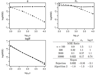
Figure 2: Comparisons of rejection (solid) and iterative importance sampling (dashed) versions of approximate Bayesian computation. For each $n$, the logarithm of the average mean square error across $100$ datasets is reported. For each dataset, the Monte Carlo sample size is $40000$. Ratios of mean square errors of the two methods are given in the table, and smaller values indicate better performance of iterative importance sampling. For each polyline in the plots, a line is fitted and the slope is reported in the table. Smaller values indicate faster decrease of the mean square error.

Approximate Bayesian computation can be used to obtain an off-line estimator for the unknown parameters of this model. Here we illustrate the effectiveness of iteratively choosing the importance proposal for large $n$ by comparing with rejection sampling. In the iterative algorithm, a $t$ distribution with 5 degrees of freedom is used to construct $q_{k}$.

Consider estimating the parameter $(\phi,\sigma_{\eta},\log\overline{\sigma})$ under a uniform prior in the region $[0,1)\times[0.1,3]\times[-10,-1]$. The setting with the true parameter $(\phi,\sigma_{\eta},\log\overline{\sigma})=(0.9,0.675,-4.1)$ is studied. We use a three-dimensional summary statistic that stores the mean, variance and lag-one autocovariance of the transformed data. If there were no noise in the state equation for $\xi_{n}^{*}$, then this would be a sufficient statistic of ${}{Y}^{*}$, and hence is a natural choice for the summary statistic. The uniform kernel is used in the accept-reject step.

We evaluate rejection sampling and iterative importance sampling methods on data of length $n=100,500,2000$ and $10000$; and use $N=40000$ Monte Carlo simulations. For iterative importance sampling, the sequence $\{p_{k}\}$ has the first five values decreasing linearly from $5\%$ to $1\%$, and later values being $1\%$. We further set $N_{0}=2000$, and $K_{\rm max}=10$. For the rejection sampler acceptance probabilities of both $5\%$ and $1\%$ were tried and $5\%$ was chosen as it gave better performance. The simulation results are shown in Figure 2.

For all parameters, iterative importance sampling shows increasing advantage over rejection sampling as $n$ increases. For larger $n$, the iterative procedure obtains a center for proposals closer to the true parameter and a bandwidth that is smaller than those used for rejection sampling. These contribute to the more accurate estimators. It is easy to estimate $\log\bar{\sigma}$, since the expected summary statistic $\widetilde{E}({}{Y}^{*})$ is roughly linear in $\log\bar{\sigma}$. Thus iterative importance sampling has less of an advantage over rejection sampling when estimating this parameter.

6 Discussion

Our results suggest one can obtain efficient estimates using Approximate Bayesian Computation with a fixed Monte Carlo sample size as $n$ increases. Thus the computational complexity of approximate Bayesian computation will just be the complexity of simulating a sample of size $n$ from the underlying model.

Our results on the Monte Carlo accuracy of approximate Bayesian computation considered the importance sampling implementation given in Algorithm 1. If we do not use the uniform kernel, then there is a simple improvement on this algorithm, that absorbs the accept-reject probability within the importance sampling weight. A simple Rao–Blackwellisation argument then shows that this leads to a reduction in Monte Carlo variance, so our positive results about the scaling of approximate Bayesian computation with $n$ will also immediately apply to this implementation.

Similar positive Monte Carlo results are likely to apply to Markov chain Monte Carlo implementations of approximate Bayesian computation. A Markov chain Monte Carlo version will be efficient provided the acceptance probability does not degenerate to zero as $n$ increases. However at stationarity, it will propose parameter values from a distribution close to the approximate Bayesian computation posterior density, and Theorems 4.5 and 4.6 suggest that for such a proposal distribution the acceptance probability will be bounded away from zero.

Whilst our theoretical results suggest that point estimates based on approximate Bayesian computation have good properties, they do not suggest that the approximate Bayesian computation posterior is a good approximation to the true posterior. In fact, Frazier et al. (2016) show it will over-estimate uncertainty if $\varepsilon_{n}=O(a_{n}^{-1})$. However, Li & Fearnhead (2018) show that using regression methods Beaumont et al. (2002) to post-process approximate Bayesian computation output can lead to both efficient point estimation and accurate quantification of uncertainty.

Supplementary Material

7 Proof of Results from Section 3

7.1 Overview and Notation

We first give an overview of the proof to Theorem 3.1. The convergence of the maximum likelihood estimator based on the summary follows almost immediately from Creel & Kristensen (2013). The minor extensions we used are summarized in Lemmas 7.1 and 7.2 below.

The main challenge with Theorem 3.1 are the results about the posterior mean of approximate Bayesian computation. For the convergence of posterior means of approximate Bayesian computation we need to consider convergence of integrals over the parameter space, $\mathbbm{R}^{p}$. We will divide $\mathbbm{R}^{p}$ into $B_{\delta}=\{\theta:\|\theta-\theta_{0}\|<\delta\}$ and $B_{\delta}^{c}$ for some $\delta<\delta_{0}$, and introduce the notation $\pi(h)=\int h(\theta)\pi(\theta)f_{\rm ABC}(s_{{\rm obs}}\mid\theta)\,d\theta$. The posterior mean of approximate Bayesian computation is $h_{\rm ABC}=\pi(h)/\pi(1)$. We can write $\pi(h)$, say, as $\pi(h)=\pi_{B_{\delta}}(h)+\pi_{B_{\delta}^{c}}(h)$, where

$$\pi_{B_{\delta}}(h)=\int_{B_{\delta}}h(\theta)\pi(\theta)f_{\rm ABC}(s_{{\rm obs}}\mid\theta)\,d\theta,\quad\pi_{B_{\delta}^{c}}(h)=\int_{B_{\delta}^{c}}h(\theta)\pi(\theta)f_{\rm ABC}(s_{{\rm obs}}\mid\theta)\,d\theta.$$

As $n\rightarrow\infty$ the posterior distribution of approximate Bayesian computation concentrates around $\theta_{0}$. The first step of our proof is to show that, as a result, the contribution that comes from integrating over $B_{\delta}^{c}$ can be ignored. Hence we need consider only $\pi_{B_{\delta}}(h)/\pi_{B_{\delta}}(1)$.

Second, we perform a Taylor expansion of $h(\theta)$ around $\theta_{0}$. Let $Dh(\theta)$ and $Hh(\theta)$ denote the vector of first derivatives and the matrix of second derivatives of $h(\theta)$ respectively. Then

$$h(\theta)=h(\theta_{0})+Dh(\theta_{0})^{T}(\theta-\theta_{0})+\frac{1}{2}(\theta-\theta_{0})^{T}Hh(\theta_{*})(\theta-\theta_{0}),$$

for some $\theta_{*}$, that depends on $\theta$ and that satisfies $||\theta_{*}-\theta_{0}||<||\theta-\theta_{0}||$. We plug this into $\pi_{B_{\delta}}(h)$, but re-express the integrals in term of the rescaled random vector

$$t(\theta)=a_{n,\varepsilon}(\theta-\theta_{0}),$$

and let $t(B_{\delta})$ be the set $\{\phi:\phi=t(\theta)\text{ for some }\theta\in B_{\delta}\}$. This gives

$$\frac{\pi_{B_{\delta}}(h)}{\pi_{B_{\delta}}(1)}=h(\theta_{0})+a_{n,\varepsilon}^{-1}Dh(\theta_{0})^{T}\frac{\pi_{B_{\delta}}(t)}{\pi_{B_{\delta}}(1)}+\frac{1}{2}a_{n,\varepsilon}^{-2}\frac{\pi_{B_{\delta}}\{t^{T}Hh(\theta_{t})t\}}{\pi_{B_{\delta}}(1)},$$ (5)

where we write $t$ for $t(\theta)$, and $\theta_{t}$ is the value $\theta_{*}$ from remainder term in the Taylor expansion for $h(\theta)$. We use the notation $\theta_{t}$ to emphasize its dependence on $t$, and note that $\theta_{t}$ belongs to $B_{\delta}$.

Let $\widetilde{f}_{\rm ABC}(s_{{\rm obs}}\mid\theta)=\int\widetilde{f}_{n}(s_{{\rm obs}}+\varepsilon_{n}v\mid\theta)K(v)\,dv$, which is the likelihood approximation that we get if we replace the true likelihood by its Gaussian limit, and define $\widetilde{\pi}_{B_{\delta}}(h)=\int_{B_{\delta}}h(\theta)\pi(\theta)\widetilde{f}_{\rm ABC}(s_{{\rm obs}}\mid\theta)\,d\theta$. Our third step is to re-write (5) as

$$\frac{\pi_{B_{\delta}}(h)}{\pi_{B_{\delta}}(1)} = h(\theta_{0})+a_{n,\varepsilon}^{-1}Dh(\theta_{0})^{T}\frac{\widetilde{\pi}_{B_{\delta}}(t)}{\widetilde{\pi}_{B_{\delta}}(1)}+a_{n,\varepsilon}^{-1}Dh(\theta_{0})^{T}\left\{\frac{\widetilde{\pi}_{B_{\delta}}(t)}{\widetilde{\pi}_{B_{\delta}}(1)}-\frac{\pi_{B_{\delta}}(t)}{\pi_{B_{\delta}}(1)}\right\}$$

$$+\frac{1}{2}a_{n,\varepsilon}^{-2}\frac{\pi_{B_{\delta}}\{t^{T}Hh(\theta_{t})t\}}{\pi_{B_{\delta}}(1)}.$$

We bound the size of the last two terms, so that asymptotically $h_{\rm ABC}$ behaves as

$$h(\theta_{0})+a_{n,\varepsilon}^{-1}Dh(\theta_{0})^{T}\frac{\widetilde{\pi}_{B_{\delta}}(t)}{\widetilde{\pi}_{B_{\delta}}(1)}.$$

If we introduce the density $g_{n}(t,v)$, defined as $g_{n}(t,v,\tau)$ in Section 4.3 of the main text but with $\tau=0$, so

$$g_{n}(t,v)\propto\begin{cases}\begin{array}[]{c}N\Big{\{}Ds(\theta_{0})t;a_{n}\varepsilon_{n}v+A(\theta_{0})^{1/2}T_{\rm obs},A(\theta_{0})\Big{\}}K(v),\quad a_{n}\varepsilon_{n}\rightarrow c<\infty,\\ N\Big{\{}Ds(\theta_{0})t;v+\frac{1}{a_{n}\varepsilon_{n}}A(\theta_{0})^{1/2}T_{\rm obs},\frac{1}{a_{n}^{2}\varepsilon_{n}^{2}}A(\theta_{0})\Big{\}}K(v),\quad a_{n}\varepsilon_{n}\rightarrow\infty,\end{array}\end{cases}$$

then we can show that

$$\frac{\widetilde{\pi}_{B_{\delta}}(t)}{\widetilde{\pi}_{B_{\delta}}(1)}\approx\frac{\int_{t(B_{\delta})}\int_{\mathbb{R}^{d}}tg_{n}(t,v)\,dtdv}{\int_{t(B_{\delta})}\int_{\mathbb{R}^{d}}g_{n}(t,v)\,dtdv},$$

with a remainder that can be ignored. Putting this together, we get that asymptotically $h_{\rm ABC}$ is

$$h(\theta_{0})+a_{n,\varepsilon}^{-1}Dh(\theta_{0})^{T}\frac{\int_{t(B_{\delta})}\int_{\mathbb{R}^{d}}tg_{n}(t,v)\,dtdv}{\int_{t(B_{\delta})}\int_{\mathbb{R}^{d}}g_{n}(t,v)\,dtdv},$$

and the proof finishes by calculating the form of this.

A recurring theme in the proofs for the bounds on the various remainders is the need to bound expectations of polynomials of either the rescaled parameter $t$, or a rescaled difference in the summary statistic from $s_{{\rm obs}}$, or both. Later we will present a lemma, stated in terms of a general polynomial, that is used repeatedly to obtain the bounds we need.

To define this we need to introduce a set of suitable polynomials. For any integer $l$ and vector $x$, if a scalar function of $x$ has the expression $\sum_{i=0}^{l}\alpha_{i}(x,n)^{T}x^{i}$, where for each $i$, $x^{i}$ denotes the vector with all monomials of $x$ with degree $i$ as elements and $\alpha_{i}(x,n)$ is a vector of functions of $x$ and $n$, we denote it by $P_{l}(x)$. Let $\mathbb{P}_{l,x}$ be the set

$$\{P_{l}(x):\text{for all }i\leq l,\ \text{as }n\rightarrow\infty,\ \alpha_{i}(x,n)=O_{p}(1)\text{ holds uniformly in }x\}$$

To simplify the notations, for two vectors $x_{1}$ and $x_{2}$, $P_{l}\{(x_{1}^{T},x_{2}^{T})^{T}\}$ and $\mathbb{P}_{l,(x_{1}^{T},x_{2}^{T})^{T}}$ are written as $P_{l}(x_{1},x_{2})$ and $\mathbb{P}_{l,(x_{1},x_{2})}$. Where the specific form of the polynomial does not matter, and we only use the fact that it lies in $\mathbb{P}_{l,x}$, we will often simplify expressions by writing it as $P_{l}(x)$.

7.2 Proof of Theorem 3.1

For the maximum likelihood estimator based on the summary, Creel & Kristensen (2013) gives the central limit theorem for $\hat{\theta}_{\mbox{\scriptsize\rm MLES}}$ when $a_{n}={n}^{1/2}$ and $\mathcal{P}$ is compact. According to the proof in Creel & Kristensen (2013), extending the result to the general $a_{n}$ is straightforward. Additionally, we give the extension for general $\mathcal{P}$.

Lemma 7.1.

Assume Conditions 2,2-2. Then $a_{n}(\hat{\theta}_{\mbox{\scriptsize\rm MLES}}-\theta_{0})\rightarrow N\{0,I^{-1}(\theta_{0})\}$ in distribution as $n\rightarrow\infty$.

Given Condition 2, by Lemma 7.1 and the delta method Lehmann (2004), the convergence of the maximum likelihood estimator for general $h(\theta)$ holds as follows.

Lemma 7.2.

Assume the conditions of Lemma 7.1 and Condition 2. Then $a_{n}\{h(\hat{\theta}_{\mbox{\scriptsize\rm MLES}})-h(\theta_{0})\}\rightarrow N\{0,Dh(\theta_{0})^{T}I^{-1}(\theta_{0})Dh(\theta_{0})\}$ in distribution as $n\rightarrow\infty$.

The following lemmas are used for the result about the posterior mean of approximate Bayesian computation, proofs of these are given in Section 7.3. Our first lemma is used to justify ignoring integrals over ${B_{\delta}^{c}}$.

Lemma 7.3.

Assume Conditions 2, 2–2. Then for any $\delta<\delta_{0},$ $\pi_{B_{\delta}^{c}}(h)=O_{p}(e^{-a_{n,\varepsilon}^{\alpha_{\delta}}c_{\delta}})$ for some positive constants $c_{\delta}$ and $\alpha_{\delta}$ depending on $\delta$.

The following lemma is used to calculate the form of

$$\frac{\int_{t(B_{\delta})}\int_{\mathbb{R}^{d}}tg_{n}(t,v)\,dtdv}{\int_{t(B_{\delta})}\int_{\mathbb{R}^{d}}g_{n}(t,v)\,dtdv},$$

which is the leading term for $\{h_{\rm ABC}-h(\theta_{0})\}$.

Lemma 7.4.

Assume Condition 2. Let $c$ be a constant vector, $\{k_{n}\}$ be a series converging to $k_{\infty}\in(0,\infty]$ and $\{b_{n}^{\prime}\}$ be a series converging to a non-negative constant. Let $b_{n}=\mathbbm{1}_{\{k_{\infty}=\infty\}}+b_{n}^{\prime}\mathbbm{1}_{\{k_{\infty}<\infty\}}$. Then for any $d\times p$ constant matrix $A$ and any $d\times d$ constant matrix $B$,

$$\int_{\mathbb{R}^{p}}\int_{\mathbb{R}^{d}}t\frac{N(At;B_{n}v+\frac{1}{k_{n}}c,\frac{1}{k_{n}^{2}}I_{d})K(v)}{\int_{\mathbb{R}^{p}}\int_{\mathbb{R}^{d}}N(At;B_{n}v+\frac{1}{k_{n}}c,\frac{1}{k_{n}^{2}}I_{d})K(v)\,dtdv}\,dtdv=\frac{1}{k_{n}}\left\{(A^{T}A)^{-1}A^{T}c+R(A,B_{n},k_{n},c)\right\},$$

where $B_{n}=b_{n}B$, the expression of $R(c;A,B_{n},k_{n})$ is stated in the proof. Specifically, $R(A,B_{n},k_{n},c)=o(1)$ when $B_{n}=o(1)$ and $O(1)$ otherwise.

Our final two lemmas are used to bound the remainder terms in the expansion for $h_{\rm ABC}$ we presented in Section 7.1.

Lemma 7.5.

Assume Conditions 2, 2 and 2 hold. If $\varepsilon_{n}=o({a_{n}}^{-1/2})$, there exists a $\delta<\delta_{0}$ such that

$$\widetilde{\pi}_{B_{\delta}}(1)=a_{n,\varepsilon}^{d-p}\Big{\{}\pi(\theta_{0})\int_{t(B_{\delta})}\int_{\mathbb{R}^{d}}g_{n}(t,v)\,dvdt+O_{p}(a_{n,\varepsilon}^{-1})+O_{p}(a_{n}^{2}\varepsilon_{n}^{4})\Big{\}},$$

$$\int_{t(B_{\delta})}\int_{\mathbb{R}^{d}}g_{n}(t,v)\,dtdv=\Theta_{p}(1),$$

$$\frac{\widetilde{\pi}_{B_{\delta}}(t)}{\widetilde{\pi}_{B_{\delta}}(1)}=\frac{\int_{t(B_{\delta})}\int_{\mathbb{R}^{d}}tg_{n}(t,v)\,dtdv}{\int_{t(B_{\delta})}\int_{\mathbb{R}^{d}}g_{n}(t,v)\,dtdv}+O_{p}(a_{n,\varepsilon}^{-1})+O_{p}(a_{n}^{2}\varepsilon_{n}^{4}),$$ (6)

and $\widetilde{\pi}_{B_{\delta}}\{P_{2}(t)\}/\widetilde{\pi}_{B_{\delta}}(1)=O_{p}(1)$ for any $P_{2}(t)\in\mathbb{P}_{2,t}$.

Lemma 7.6.

Assume the conditions of Lemma 7.5 and Conditions 2 and 2. Then if $\varepsilon_{n}=o({a_{n}}^{-1/2})$, there exists a $\delta<\delta_{0}$ such that

$$\frac{\pi_{B_{\delta}}(h)}{\pi_{B_{\delta}}(1)}=h(\theta_{0})+a_{n,\varepsilon}^{-1}Dh(\theta_{0})^{T}\left\{\frac{\widetilde{\pi}_{B_{\delta}}(t)}{\widetilde{\pi}_{B_{\delta}}(1)}+O_{p}(\alpha_{n}^{-1})\right\}+\frac{1}{2}a_{n,\varepsilon}^{-2}\left[\frac{\widetilde{\pi}_{B_{\delta}}\{t^{T}Hh(\theta_{t})t\}}{\widetilde{\pi}_{B_{\delta}}(1)}+O_{p}(\alpha_{n}^{-1})\right],$$ (7)

Now we are ready to prove Theorem 3.1.

Proof 7.7 (of Theorem 3.1).

The convergence of the maximum likelihood estimator based on the summary is given by Lemma 7.1 and Lemma 7.2.

We now focus on the convergence for the posterior mean of approximate Bayesian computation. The convergence of the posterior mean given the summaries follows from a similar, but simpler, argument and is omitted.

We can bound $t^{T}H(\theta_{t})t$ for $\theta$ in $B_{\delta}$ by the quadratic $t^{T}H_{max}t$, where $H_{max}$ is an upper bound on $H(\theta_{t})$ for $\theta_{t}$ in $B_{\delta}$. This means that

$$\widetilde{\pi}_{B_{\delta}}\{t^{T}Hh(\theta_{t})t\}=O(1).$$

Together with Lemmas 7.3, 7.5 and 7.6, we then have the expansion

$$h_{\rm ABC}=h(\theta_{0})+a_{n,\varepsilon}^{-1}Dh(\theta_{0})^{T}\left\{\frac{\int_{t(B_{\delta})\times\mathbb{R}^{d}}tg_{n}(t,v)\,dtdv}{\int_{t(B_{\delta})\times\mathbb{R}^{d}}g_{n}(t,v)\,dtdv}+O_{p}(a_{n,\varepsilon}^{-1})+O_{p}(a_{n}^{2}\varepsilon_{n}^{4})+O_{p}(\alpha_{n}^{-1})\right\}.$$

The analytical form of the integral in the above expansion, which we will denote by $E_{g_{n}}(t)$, can be obtained by applying Lemma 7.4 with $A=A(\theta_{0})^{-1/2}DS(\theta_{0})$, $c=T_{{\rm obs}}$,

$$B_{n}=\begin{cases}a_{n}\varepsilon_{n}A(\theta_{0})^{-1/2},&c_{\varepsilon}<\infty,\\ A(\theta_{0})^{-1/2},&c_{\varepsilon}=\infty,\end{cases}\quad k_{n}=\begin{cases}1,&c_{\varepsilon}<\infty,\\ a_{n}\varepsilon_{n},&c_{\varepsilon}=\infty.\end{cases}$$

It can be seen that $E_{g_{n}}(t)$ is $\Theta_{p}(k_{n}^{-1})$, and the remainder term, $O_{p}(a_{n,\varepsilon}^{-1})+O_{p}(a_{n}^{2}\varepsilon_{n}^{4})+O_{p}(\alpha_{n}^{-1})$, is $o_{p}(1)$ as $\varepsilon_{n}=o(a_{n}^{-3/5})$ and $\alpha_{n}^{-1}=o(a_{n}^{-2/5})$. Then since $a_{n,\varepsilon}^{-1}k_{n}^{-1}=a_{n}^{-1}$, we have

$$a_{n}\{h_{\rm ABC}-h(\theta_{0})\}$$

$$= Dh(\theta_{0})^{T}\Big{[}\Big{\{}Ds(\theta_{0})^{T}A(\theta_{0})^{-1}Ds(\theta_{0})\Big{\}}^{-1}Ds(\theta_{0})^{T}A(\theta_{0})^{-1/2}T_{{\rm obs}}+R_{n}(a_{n}\varepsilon_{n},T_{\rm obs})\Big{]}+o_{p}(1),$$ (8)

where $R_{n}(a_{n}\varepsilon_{n},T_{\rm obs})$ is $Dh(\theta_{0})^{T}R(A,B_{n},k_{n},c)$ with $R(A,B_{n},k_{n},c)$ defined in Lemma 7.4. We can interpret $R_{n}(a_{n}\varepsilon_{n},T_{\rm obs})$ as the extra variation brought by $\varepsilon_{n}$: $a_{n}[h_{\rm ABC}-{E}\{h(\theta)\mid s_{{\rm obs}}\}]$.

By the delta method, the first term in the right hand side of (8) converges to $I(\theta_{0})^{-1/2}Z$. For the second term, since $A(A^{T}A)^{-1}A^{T}$ is a projection matrix, by eigen decompositition

$$I-A(A^{T}A)^{-1}A^{T}=U\left(\begin{array}[]{cc}0&0\\ 0&I_{d-p}\end{array}\right)U^{T},\ (A^{T}A)^{-1/2}A^{T}=\left(\begin{array}[]{cc}I_{p}&0\\ 0&0\end{array}\right)U^{T},$$

where $U$ is an orthogonal matrix. For a vector $x$, let $x_{k_{1}:k_{2}}$ be the $(k_{2}-k_{1}+1)$-dimension vector containing the $k_{1}$th–$k_{2}$th coordinates of $x$. Let $v^{\prime}=U^{T}A(\theta_{0})^{-1/2}v$, and $T_{{\rm obs}}^{\prime}=U^{T}T_{{\rm obs}}$. Then $R_{n}(a_{n}\varepsilon_{n},T_{\rm obs})$ can be written as

$$R_{n}(a_{n}\varepsilon_{n},T_{\rm obs})$$

$$= Dh(\theta_{0})^{T}(A^{T}A)^{-1/2}a_{n}\varepsilon_{n}\frac{\int v_{1:p}^{\prime}N\{v_{(p+1):d}^{\prime};-\frac{1}{a_{n}\varepsilon_{n}}T_{{\rm obs},(p+1):d}^{\prime},\frac{1}{a_{n}^{2}\varepsilon_{n}^{2}}I_{d-p}\}K\{A(\theta_{0})^{1/2}Uv^{\prime}\}\,dv^{\prime}}{\int N\{v_{(p+1):d}^{\prime};-\frac{1}{a_{n}\varepsilon_{n}}T_{{\rm obs},(p+1):d}^{\prime},\frac{1}{a_{n}^{2}\varepsilon_{n}^{2}}I_{d-p}\}K\{A(\theta_{0})^{1/2}Uv^{\prime}\}\,dv^{\prime}}.$$ (9)

Denote the weak limit of $R_{n}(a_{n}\varepsilon_{n},T_{\rm obs})$ as $R(c_{\varepsilon},Z)$. When $d=p$, obviously $R_{n}(a_{n}\varepsilon_{n},T_{\rm obs})=0$ and therefore $R(c_{\varepsilon},Z)=0$. When $d>p$, if $\varepsilon_{n}=o(1/a_{n})$, $R_{n}(a_{n}\varepsilon_{n},T_{\rm obs})=o_{p}(1)$ by Lemma 7.4 and therefore $R(c_{\varepsilon},Z)=0$. When the covariance matrix of $K(\cdot)$ is $c^{2}A(\theta_{0})$, for constant $c>0$, $K(v)\propto\overline{K}\{c\|A(\theta_{0})^{-1/2}v\|^{2}\}$. Then $K\{A(\theta_{0})^{1/2}Uv^{\prime}\}$ in (9) can be replaced by $\overline{K}(c\|v^{\prime}\|^{2})$ and for fixed $v_{(p+1):d}^{\prime}$, the integrand in the numerator, as a function of $v_{1:p}^{\prime}$, is symmetric around zero. Therefore $R_{n}(a_{n}\varepsilon_{n},T_{\rm obs})=0$ and $R(c_{\varepsilon},Z)=0$.

Otherwise, $R_{n}(a_{n}\varepsilon_{n},z)$ is not necessarily zero. Since for any $n$, $R_{n}(a_{n}\varepsilon_{n},z)$ as a function of $z$ is symmetric around $0$, $R(c_{\varepsilon},z)$ is also symmetric and $R(c_{\varepsilon},Z)$ has mean zero. Since $I^{-1}(\theta_{0})$ is the Cramer-Rao lower bound, $\mbox{var}\{I(\theta_{0})^{-1/2}Z+R(c_{\varepsilon},Z)\}\geq I^{-1}(\theta_{0})$.

For (i), the asymptotic normality holds for $h(\hat{{\theta}})$ by Lemma 7.2.

7.3 Proof of Lemmas

Here we give the proofs of lemmas from Section 7.2.

Proof 7.8 (of Lemma 7.3).

It is sufficient to show that for any $\delta$, $\sup_{\theta\in B_{\delta}^{c}}f_{\rm ABC}(s_{{\rm obs}}\mid\theta)=O_{p}(e^{-a_{n,\varepsilon}^{\alpha_{\delta}}c_{\delta}})$. By dividing $\mathbb{R}^{d}$ into $\{v:\|\varepsilon_{n}v\|\leq\delta^{\prime}/3\}$ and its complement, we have

$$\sup_{\theta\in B_{\delta}^{c}}f_{\rm ABC}(s_{{\rm obs}}\mid\theta)=\sup_{\theta\in B_{\delta}^{c}}\int_{\mathbb{R}^{d}}f_{n}(s_{{\rm obs}}+\varepsilon_{n}v\mid\theta)K(v)\,dv$$

$$\leq \sup_{\theta\in B_{\delta}^{c}\backslash\mathcal{P}_{0}^{c}}\left\{\sup_{\|s-s_{{\rm obs}}\|\leq\delta^{\prime}/3}f_{n}(s\mid\theta)\right\}+\sup_{\theta\in\mathcal{P}_{0}^{c}}\left\{\sup_{\|s-s_{{\rm obs}}\|\leq\delta^{\prime}/3}f_{n}(s\mid\theta)\right\}+\bar{K}(\lambda_{\min}(\Lambda)\varepsilon_{n}^{-1}\delta^{\prime}/3)\varepsilon_{n}^{-d},$$

where $\lambda_{\min}(\Lambda)$ is positive. In the above, as $n\rightarrow\infty$, the third term is exponentially decreasing by Conditions 2(iv). For the second term, by Condition 2, with probability $1$,

$$\|s-s(\theta)\| =\|\{s(\theta_{0})-s(\theta)\}+\{s_{\rm obs}-s(\theta_{0})\}+\varepsilon_{n}v\|$$

$$\geq\delta^{\prime}-\delta^{\prime}/3-\delta^{\prime}/3=\delta^{\prime}/3.$$

Recall that $W_{n}(s)=a_{n}A(\theta)^{-1/2}\{s-s(\theta)\}$. Then by Condition 2, the second term is exponentially decreasing. For the first term, when $\theta\in B_{\delta}^{c}\backslash\mathcal{P}_{0}^{c}$ and $\|s-s_{{\rm obs}}\|\leq\delta^{\prime}/3$, $\|W_{n}(s)\|\geq a_{n}\delta^{\prime}r$ for some constant $r$. By Condition 2 and 2, $f_{W_{n}}(w\mid\theta)$ is bounded by the sum of a normal density and $\alpha_{n}^{-1}r_{{\rm max}}(w)$, which are both exponentially decreasing, so $\sup_{\theta\in B_{\delta}^{c}\backslash\mathcal{P}_{0}^{c}}\sup_{\|s-s_{{\rm obs}}\|\leq\delta^{\prime}/3}f_{n}(s\mid\theta)$ is also exponentially decreasing. Finally, the sum of all the above is $O(e^{-a_{n,\varepsilon}^{\alpha_{\delta}}c_{\delta}})$ by noting that $a_{n,\varepsilon}\leq\min(\varepsilon_{n}^{-1},a_{n})$.

The following additional lemma will be used repeatedly to bound error terms that appear in Lemmas 7.5 and 7.6.

Lemma 7.9.

Assume Condition 2. For $t\in\mathbb{R}^{p}$ and $v\in\mathbb{R}^{d}$, let $\{A_{n}(t)\}$ be a series of $d\times p$ matrix functions, $\{C_{n}(t)\}$ be a series of $d\times d$ matrix functions, $Q$ be a positive definite matrix and $g_{1}(v)$ and $g_{2}(v)$ be probability densities in $\mathbb{R}^{d}$. Let $c$ be a random vector, $\{k_{n}\}$ be a series converging to $k_{\infty}\in(0,\infty]$ and $\{b_{n}^{\prime}\}$ be a series converging to a non-negative constant. Let $b_{n}=\mathbbm{1}_{\{k_{\infty}=\infty\}}+b_{n}^{\prime}\mathbbm{1}_{\{k_{\infty}<\infty\}}$. If

(i) $g_{1}(v)$ and $g_{2}(v)$ are bounded in $\mathbb{R}^{d}$;

(ii) $g_{1}(v)$ and $g_{2}(v)$ depend on $v$ only through $\|v\|$ and are decreasing functions of $\|v\|$;

(iii) there exists an integer $l$ such that $\int\prod_{k=1}^{l+p}v_{i_{k}}g_{j}(v)\,dv<\infty$, $j=1,2$, for any coordinates $(v_{i_{1}},\cdots,v_{i_{l}})$ of $v$;

(iv) there exists a positive constant $m$ such that for any $t\in\mathbb{R}^{p}$ and $n$, $\lambda_{{\rm min}}\{A_{n}(t)\}$ and $\lambda_{{\rm min}}\{C_{n}(t)\}$ are greater than $m$;

then for any $P_{l}(t,v)\in\mathbb{P}_{l,(t,v)}$,

$$\int_{\mathbb{R}^{p}}\int_{\mathbb{R}^{d}}P_{l}(t,v)k_{n}^{d}g_{1}[k_{n}C_{n}(t)\{A_{n}(t)t-b_{n}v-k_{n}^{-1}c\}]g_{2}(Qv)\,dvdt =O_{p}(1),$$

$$\int_{\mathbb{R}^{p}}\int_{\mathbb{R}^{d}}k_{n}^{d}g_{1}[k_{n}C_{n}(t)\{A_{n}(t)t-b_{n}v-k_{n}^{-1}c\}]g_{2}(Qv)\,dvdt =\Theta_{p}(1).$$

Proof 7.10.

For simplicity, here $\int$ denotes the integration over the whole Euclidean space. According to (ii), $g_{1}(v)$ can be written as $\bar{g}_{1}(\|v\|)$. When $k_{\infty}<\infty$, assume $k_{n}=1$ without loss of generality. For any $P_{l}(t,v)\in\mathbb{P}_{l,(t,v)}$, by Cauchy–Schwarz inequality, there exists a $P_{l}(\|t\|,\|v\|)\in\mathbb{P}_{l,(\|t\|,\|v\|)}$ with coefficient functions taking positive values such that $|P_{l}(t,v)|$ is bounded by $P_{l}(\|t\|,\|v\|)$ almost surely. Therefore for the first equality, it is sufficient to consider the equality where $P_{l}(t,v)$ is replaced by $P_{l}(\|t\|,\|v\|)$ and the coefficient functions of $P_{l}(\|t\|,\|v\|)$ are positive almost surely. For each $n$, divide $\mathbb{R}^{p}$ into $V=\{t:\|A_{n}(t)t\|/2\geq\|b_{n}^{\prime}v+c\|\}$ and $V^{c}$. In $V$, $\|C_{n}(t)\{A_{n}(t)t-b_{n}^{\prime}v-c\}\|\geq m^{2}\|t\|/2$; in $V^{c}$, $\|t\|\leq 2m^{-1}\|b_{n}^{\prime}v+c\|$. With probability tending to $1$,

$$\int P_{l}(\|t\|,\|v\|)g_{1}[C_{n}(t)\{A_{n}(t)t-b_{n}^{\prime}v-c\}]g_{2}(Qv)\,dvdt\leq$$

$$\int P_{l}(\|t\|,\|v\|)\bar{g}_{1}(m^{2}\|t\|/2)g_{2}(Qv)\,dvdt+\sup_{v\in\mathbb{R}^{d}}g_{1}(v)\int\int_{V^{c}}dt\,P_{l}(2m^{-1}\|b_{n}^{\prime}v+c\|,\|v\|)g_{2}(Qv)\,dv.$$

In the above, $\int_{V^{c}}\,dt$ is the volume of $V^{c}$ in $\mathbb{R}^{p}$ and is proportional to $\|b_{n}^{\prime}v+c\|^{p}$. By (iii), the right hand side of the above inequality is $O_{p}(1)$.

When $k_{\infty}=\infty$, let $v^{*}=k_{n}\{A(t)t-v-k_{n}^{-1}c\}$. Then for any $P_{l}(t,v)\in\mathbb{P}_{l,(t,v)}$, with probability $1$,

$$\left|\int P_{l}(t,v)k_{n}^{d}g_{1}[k_{n}C_{n}(t)\{A(t)t-v-k_{n}^{-1}c\}]g_{2}(Qv)\,dvdt\right|$$

$$= \left|\int P_{l}(t,v^{*})g_{2}[Q\{A(t)t-k_{n}^{-1}v^{*}-k_{n}^{-1}c\}]g_{1}(C_{n}(t)v^{*})\,dv^{*}dt\right|,$$

$$\leq \int P_{l}(\|t\|,\|v^{*}\|)g_{2}[Q\{A(t)t-k_{n}^{-1}v^{*}-k_{n}^{-1}c\}]\overline{g}_{1}(m\|v^{*}\|)\,dv^{*}dt$$

for some $P_{l}(t,v^{*})\in\mathbb{P}_{l,(t,v^{*})}$ and $P_{l}(\|t\|,\|v^{*}\|)\in\mathbb{P}_{l,(\|t\|,\|v^{*}\|)}$. The right hand side of the above inequality is similar to the integral when $k_{\infty}<\infty$ with $g_{1}(\cdot)$ and $g_{2}(\cdot)$ replaced by $g_{2}(\cdot)$ and $\overline{g}_{1}(\cdot)$ respectively. Therefore it is $O_{p}(1)$ by the same reasoning.

For $P_{l}(t,v)=1$, by considering only the integral in a compact region, it is easy to see the target integral is larger than $0$. Therefore the lemma holds.

Proof 7.11 (of Lemma 7.4).

Let $P=A^{T}A$. By matrix algebra,

$$N\Big{(}At;B_{n}v+\frac{1}{k_{n}}c,\frac{1}{k_{n}^{2}}I_{d}\Big{)}K(v)=N\Big{\{}t;P^{-1}A^{T}\left(B_{n}v+\frac{1}{k_{n}}c\right),\frac{1}{k_{n}^{2}}P^{-1}\Big{\}}r(v;A,B_{n,}k_{n},c),$$

where

$$r(v;A,B_{n,}k_{n},c) =\frac{k_{n}^{d-p}}{(2\pi)^{(d-p)/2}}\exp\Big{\{}-\frac{k_{n}^{2}}{2}\left(B_{n}v+\frac{c}{k_{n}}\right)^{T}(I-AP^{-1}A^{T})\left(B_{n}v+\frac{c}{k_{n}}\right)\Big{\}}K(v).$$

Then the target integral can be expanded as

$$\int t\frac{N(At;B_{n}v+\frac{1}{k_{n}}c,\frac{1}{k_{n}^{2}}I_{d})K(v)}{\int N(At;B_{n}v+\frac{1}{k_{n}}c,\frac{1}{k_{n}^{2}}I_{d})K(v)\,dtdv}\,dtdv =\int P^{-1}A^{T}\left(\frac{1}{k_{n}}c+B_{n}v\right)\frac{r(v;A,B_{n,}k_{n},c)}{\int r(v;A,B_{n,}k_{n},c)\,dv}\,dv$$

$$=\frac{1}{k_{n}}\left\{(A^{T}A)^{-1}A^{T}c+R(A,B_{n},k_{n},c)\right\},$$

where

$$R(A,B_{n},k_{n},c)=(A^{T}A)^{-1}A^{T}B_{n}\int k_{n}v\frac{r(v;A,B_{n,}k_{n},c)}{\int r(v;A,B_{n,}k_{n},c)\,dv}\,dv.$$

The remainder term $R(A,B_{n},k_{n},c)$ depends on the mean of the probability density proportional to $r(v;A,B_{n,}k_{n},c)$ in the directions of $(A^{T}A)^{-1}A^{T}B$. If $B_{n}$ does not degenerate to $0$ as $n\rightarrow\infty$, then in the directions orthogonal to those of $(I-A(A^{T}A)^{-1}A^{T})^{1/2}B$, $r(v;A,B_{n,}k_{n},c)$ is symmetric around $0$; in the directions of $(I-A(A^{T}A)^{-1}A^{T})^{1/2}B$, $r(v;A,B_{n,}k_{n},c)$ is a product of a normal density whose mean is $O(1/k_{n})$ and a rescaled $K(v)$, which is symmetric around $0$, so its mean value is $O(1/k_{n})$. Therefore when the spaces expanded by $(A^{T}A)^{-1}A^{T}B$ and $\{I-A(A^{T}A)^{-1}A^{T}\}B$ are orthogonal, $R(A,B_{n},k_{n},c)=0$; when it is not the case, $R(A,B_{n},k_{n},c)=O(1)$.

If $B_{n}=o(1)$ as $n\rightarrow\infty$, which implies $k_{n}\rightarrow c\in(0,\infty)$, it is easy to see that $\int k_{n}vr(v;A,B_{n,}k_{n},c)\,dv/\int r(v;A,B_{n,}k_{n},c)\,dv$ is upper bounded as $n\rightarrow\infty$ and hence $R(A,B_{n},k_{n},c)$ is $o(1)$.

In the following lemmas, to deal with the case where $K(x)=\bar{K}(||x||_{\Lambda})$ with $\Lambda$ not the identity, we use the property that such a $K(x)$ can be bounded above by a function that depends only on $||x||$. We refer to this bound as $K(\cdot)$ rescaled to have identity covariance matrix.

Proof 7.12 (of Lemma 7.5).

First consider $\widetilde{\pi}_{B_{\delta}}(1)$. With the transformation $t=t(\theta)$,

$$\widetilde{\pi}_{B_{\delta}}(1) =a_{n,\varepsilon}^{-p}\int_{t(B_{\delta})}\int_{\mathbb{R}^{d}}\pi(\theta_{0}+a_{n,\varepsilon}^{-1}t)\widetilde{f}_{n}(s_{{\rm obs}}+\varepsilon_{n}v\mid\theta_{0}+a_{n,\varepsilon}^{-1}t)K(v)\,dvdt.$$ (10)

We can obtain an expansion of $\widetilde{\pi}_{B_{\delta}}(1)$ by expanding $\widetilde{f}_{n}(s_{{\rm obs}}+\varepsilon_{n}v\mid\theta_{0}+a_{n,\varepsilon}^{-1}t)K(v)$ as follows. The expansion needs to be discussed separately for two cases, depending on whether the limit of $a_{n}\varepsilon_{n}$ is finite or infinite.

When $a_{n}\varepsilon_{n}\rightarrow c_{\varepsilon}<\infty$, $a_{n,\varepsilon}=a_{n}$. We apply a Taylor expansion to $s(\theta_{0}+a_{n}^{-1}t)$ and $A(\theta_{0}+a_{n}^{-1}t)^{-1/2}$ and have

$$\widetilde{f}_{n}(s_{{\rm obs}}+\varepsilon_{n}v\mid\theta_{0}+a_{n}^{-1}t)=\frac{a_{n}^{d}}{|A(\theta_{0}+a_{n}^{-1}t)|^{1/2}}$$

$$\times N\left(\Big{\{}A(\theta_{0})^{-1/2}+a_{n}^{-1}r_{A}(t,\epsilon_{2})\Big{\}}\Big{[}A(\theta_{0})^{1/2}T_{\rm obs}+a_{n}\varepsilon_{n}v-\{Ds(\theta_{0})+a_{n}^{-1}r_{s}(t,\epsilon_{1})\}t\Big{]};0,I_{d}\right),$$ (11)

where $r_{s}(t,\epsilon_{1})$ is the $d\times p$ matrix whose $i$th row is $t^{T}Hs_{i}\{\theta_{0}+\epsilon_{1}(t)\}$, $r_{A}(t,\epsilon_{2})$ is the $d\times d$ matrix $\sum_{k=1}^{p}\frac{d}{d\theta_{k}}A\{\theta_{0}+\epsilon_{2}(t)\}^{-1/2}t_{k}$, and $\epsilon_{1}(t)$ and $\epsilon_{2}(t)$ are from the remainder terms of the Taylor expansions and satisfy $\|\epsilon_{1}(t)\|\leq\delta$ and $\|\epsilon_{2}(t)\|\leq\delta$. For a $d\times d$ matrix $\tau_{2}$, let $g_{n}(t,v;\tau_{1},\tau_{2})$ be the function $g_{n}(t,v;\tau_{1})$, defined in Section 4.3 of the main text, with $A(\theta_{0})$ replaced by $\{A(\theta_{0})^{-1/2}+\tau_{2}\}^{-2}$. Applying a Taylor expansion to the normal density in (11), we have

$$\widetilde{f}_{n}(s_{{\rm obs}}+\varepsilon_{n}v\mid\theta_{0}+a_{n}^{-1}t)K(v)$$

$$= \frac{a_{n}^{d}|A(\theta_{0})|^{1/2}}{|A(\theta_{0}+a_{n}^{-1}t)|^{1/2}}\Big{[}g_{n}(t,v)+a_{n}^{-1}P_{3}(t,v)g_{n}\{t,v;e_{n1}r_{s}(t,\epsilon_{1}),e_{n1}r_{A}(t,\epsilon_{2})\}\Big{]},$$ (12)

where $P_{3}(t,v)$ is the function

$$\frac{1}{2|A(\theta_{0})^{-1/2}+r_{2}(a_{n}^{-1}t)|}$$

$$\times \left.\frac{d}{dx}\left\|\left\{A(\theta_{0})^{-1/2}+xr_{A}(t,\epsilon_{2})\right\}\left[A(\theta_{0})^{1/2}T_{\rm obs}+a_{n}\varepsilon_{n}v-\{Ds(\theta_{0})+xr_{s}(t,\epsilon_{1})\}t\right]\right\|^{2}\right|_{x=e_{n1}},$$

and $e_{n1}$ is from the remainder term of Taylor expansion and satisfies $|e_{n1}|\leq a_{n}^{-1}$ . Since $\|e_{n1}t\|\leq\delta$ and $r_{s}(t,\epsilon_{1})$ and $r_{A}(t,\epsilon_{2})$ belong $\mathbb{P}_{1,t}$, this $P_{3}(t,v)$ belongs to $\mathbb{P}_{3,(t,v)}$. Furthermore, since $r_{s}(t,\epsilon_{1})$ and $r_{A}(t,\epsilon_{2})$ have no constant term, for any small $\sigma$, $e_{n1}r_{s}(t,\epsilon_{1})$ and $e_{n1}r_{A}(t,\epsilon_{2})$ can be bounded by $\sigma I_{d}$ and $\sigma I_{p}$ uniformly in $n$ and $t$, if $\delta$ is small enough.

When $a_{n}\varepsilon_{n}\rightarrow\infty$, $a_{n,\varepsilon}=\varepsilon_{n}^{-1}$. Let $v^{*}(v)=A(\theta_{0})^{1/2}T_{{\rm obs}}+a_{n}\varepsilon_{n}v-a_{n}\varepsilon_{n}Ds(\theta_{0})t$. Under the transformation $v^{*}=v^{*}(v)$, the expansion of $\widetilde{f}_{n}(s_{{\rm obs}}+\varepsilon_{n}v\mid\theta_{0}+\varepsilon_{n}t)$ obtained by applying a Taylor expansion to $s(\theta_{0}+\varepsilon_{n}t)$ and $A(\theta_{0}+\varepsilon_{n}t)^{-1/2}$ is

$$\widetilde{f}_{n}(s_{{\rm obs}}+\varepsilon_{n}v\mid\theta_{0}+\varepsilon_{n}t)$$

$$= \frac{a_{n}^{d}}{|A(\theta_{0}+a_{n}^{-1}t)|^{1/2}}N\left[\Big{\{}A(\theta_{0})^{-1/2}+a_{n}\varepsilon_{n}^{2}\frac{r_{A}(t,\epsilon_{4})}{a_{n}\varepsilon_{n}}\Big{\}}\Big{\{}v^{*}-a_{n}\varepsilon_{n}^{2}r_{s}(t,\epsilon_{3})t\Big{\}};0,I_{d}\right],$$

where $\epsilon_{3}(t)$ and $\epsilon_{4}(t)$ are from the remainder terms of the Taylor expansion and satisfy $\|\epsilon_{3}(t)\|\leq\delta$ and $\|\epsilon_{4}(t)\|\leq\delta$. Let $g_{n}^{*}(t,v^{*};\tau_{1},\tau_{2})$ be the function

$$g_{n}^{*}(t,v^{*};\tau_{1},\tau_{2})$$

$$= N\left[v^{*};a_{n}\varepsilon_{n}\tau_{1}t,\{A(\theta_{0})^{-1/2}+\tau_{2}\}^{-2}\right]K\left\{Ds(\theta_{0})t+\frac{1}{a_{n}\varepsilon_{n}}v^{*}-\frac{1}{a_{n}\varepsilon_{n}}A(\theta_{0})^{1/2}T_{\rm obs}\right\},$$

so that $(a_{n}\varepsilon_{n})^{d}g_{n}^{*}(t,v^{*};\tau_{1},\tau_{2})$ is $g_{n}(t,v;\tau_{1},\tau_{2})$ with transformed variable $v^{*}=v^{*}(v)$, and $g_{n}^{*}(t,v^{*})=g_{n}^{*}(t,v^{*};0,0)$. Denote a $k_{1}\times k_{2}$ matrix with element being $P_{l}(t)$ by $P_{l}^{(k_{1}\times k_{2})}(t)$. Then by applying a Taylor expansion to the normal density in the expansion above,

$$\widetilde{f}_{n}(s_{{\rm obs}}+\varepsilon_{n}v\mid\theta_{0}+\varepsilon_{n}t)K(v)$$

$$= \frac{\varepsilon_{n}^{-d}|A(\theta_{0})|^{1/2}}{|A(\theta_{0}+\varepsilon_{n}t)|^{1/2}}\Big{[}g_{n}^{*}(t,v^{*})+a_{n}\varepsilon_{n}^{2}\left\{P_{2}^{(d\times 1)}(t)v^{*}+\frac{1}{a_{n}\varepsilon_{n}}v^{*T}P_{1}^{(d\times d)}(t)v^{*}\right\}g_{n}^{*}(t,v^{*})$$

$$+(a_{n}\varepsilon_{n}^{2})^{2}P_{4}(t,v^{*})g_{n}^{*}\{t,v^{*};e_{n2}r_{s}(t,\epsilon_{3}),e_{n2}r_{A}(t,\epsilon_{4})\}\Big{]}(a_{n}\varepsilon_{n})^{d},$$ (13)

where $P_{2}^{(d\times 1)}(t)$ is the function $t^{T}r_{s}(t,\epsilon_{3})^{T}A(\theta_{0})^{-1/2}/2$, $P_{1}^{(d\times d)}(t)$ is the function $-A(\theta_{0})^{-1/2}r_{A}(t,\epsilon_{4})$, $e_{n2}=e_{n2}^{\prime}/(a_{n}\varepsilon_{n})$, $e_{n2}^{\prime}$ is from the remainder term of the Taylor expansion and satisfies $|e_{n2}^{\prime}|\leq a_{n}\varepsilon_{n}^{2}$, and $P_{4}(t,v^{*})$ is a linear combination of $\{d\rho(w)/dw\}^{2}$ and $d^{2}\rho(w)/dw^{2}$ at $w=e_{n2}^{\prime}$ with $\rho(w)$ being the function

$$\Big{\|}\Big{\{}A(\theta_{0})^{-1/2}+w\frac{r_{A}(t,\epsilon_{4})}{a_{n}\varepsilon_{n}}\Big{\}}\Big{\{}v^{*}-wr_{s}(t,\epsilon_{3})t\Big{\}}\Big{\|}^{2}.$$

Obviously elements of $P_{2}^{(d\times 1)}(t)$ and $P_{1}^{(d\times d)}(t)$ belong to $\mathbb{P}_{2,t}$ and $\mathbb{P}_{1,t}$ respectively. Since $\|e_{n2}t\|\leq\delta$, the function $P_{4}(t,v^{*})$ belongs to $\mathbb{P}_{4,(t,v^{*})}$ and, similar to before, $e_{n2}r_{s}(t,\epsilon_{3})$ and $e_{n2}r_{A}(t,\epsilon_{4})$ can be bounded by $\sigma I_{d}$ and $\sigma I_{p}$ uniformly in $n$ and $t$ for any small $\sigma$, if $\delta$ is small enough.

For $\pi(\theta_{0}+a_{n,\varepsilon}^{-1}t)$ in the integral of $\widetilde{\pi}_{B_{\delta}}(1)$ in (10), a Taylor expansion gives that

$$\frac{\pi(\theta_{0}+a_{n,\varepsilon}^{-1}t)}{|A(\theta_{0}+a_{n,\varepsilon}^{-1}t)|^{1/2}} =\frac{\pi(\theta_{0})}{|A(\theta_{0})|^{1/2}}+a_{n,\varepsilon}^{-1}D_{\theta}\frac{\pi\{\theta_{0}+\epsilon_{5}(t)\}}{|A\{\theta_{0}+\epsilon_{5}(t)\}|^{1/2}}t,\quad|\epsilon_{5}(t)|\leq\delta.$$ (14)

As mentioned before, $\delta$ can be selected such that $Ds(\theta_{0})+e_{n1}r_{s}(t,\epsilon_{1})$ and $Ds(\theta_{0})+e_{n2}r_{s}(t,\epsilon_{3})$ are lower bounded by $m_{1}I_{p}$ and $A(\theta_{0})^{-1/2}+e_{n1}r_{A}(t,\epsilon_{2})$ and $A(\theta_{0})^{-1/2}+e_{n2}r_{A}(t,\epsilon_{4})$ are lowered bounded by $m_{2}I_{d}$ for some positive constant $m_{1}$ and $m_{2}$. We choose $\delta$ satisfying these and, since $\|a_{n,\varepsilon}^{-1}t\|\leq\delta$, this means $\pi(\theta_{0}+a_{n,\varepsilon}^{-1}t)/|A(\theta_{0}+a_{n,\varepsilon}^{-1}t)|^{1/2}$ is bounded uniformly in $t$ and $n$.

By plugging (12)–(14) into (10), it can be seen that the leading term of $\widetilde{\pi}_{B_{\delta}}(1)$ is $a_{n,\varepsilon}^{d-p}\pi(\theta_{0})\int_{t(B_{\delta})\times\mathbb{R}^{d}}g_{n}(t,v)\,dtdv$. The remainder terms are given in the following,

$$a_{n,\varepsilon}^{p-d}\widetilde{\pi}_{B_{\delta}}(1)-\pi(\theta_{0})\int_{t(B_{\delta})\times\mathbb{R}^{d}}g_{n}(t,v)\,dtdv$$

$$= a_{n,\varepsilon}^{-1}\int_{t(B_{\delta})\times\mathbb{R}^{d}}|A(\theta_{0})|^{1/2}D\frac{\pi(\theta_{0}+\epsilon_{5})}{|A(\theta_{0}+\epsilon_{5})|^{1/2}}tg_{n}(t,v)\,dvdt$$

$$+a_{n}^{-1}\int_{t(B_{\delta})\times\mathbb{R}^{d}}P_{3}(t,v)g_{n}\{t,v;e_{n1}r_{s}(t,\epsilon_{1}),e_{n1}r_{A}(t,\epsilon_{2})\}\,dvdt\ \mathbbm{1}_{\{\lim a_{n}\varepsilon_{n}<\infty\}}$$

$$+a_{n}\varepsilon_{n}^{2}\int_{t(B_{\delta})}P_{2}^{(d\times 1)}(t)\int_{\mathbb{R}^{d}}v^{*}g_{n}^{*}(t,v^{*})\,dv^{*}dt\ \mathbbm{1}_{\{\lim a_{n}\varepsilon_{n}=\infty\}}$$

$$+\varepsilon_{n}\int_{t(B_{\delta})\times\mathbb{R}^{d}}v^{*T}P_{1}^{(d\times d)}(t)v^{*}g_{n}^{*}(t,v^{*})\,dv^{*}dt\ \mathbbm{1}_{\{\lim a_{n}\varepsilon_{n}=\infty\}}$$

$$+a_{n}^{2}\varepsilon_{n}^{4}\int_{t(B_{\delta})\times\mathbb{R}^{d}}P_{4}(t,v^{*})g_{n}^{*}\{t,v^{*};e_{n2}r_{s}(t,\epsilon_{3}),e_{n2}r_{A}(t,\epsilon_{4})\}\,dv^{*}dt\ \mathbbm{1}_{\{\lim a_{n}\varepsilon_{n}=\infty\}},$$ (15)

where $P_{3}(t,v)$, $P_{2}^{(d\times 1)}(t)$, $P_{1}^{(d\times d)}(t)$ and $P_{4}(t,v^{*})$ are products of $\pi(\theta_{0}+a_{n,\varepsilon}^{-1}t)/|A(\theta_{0}+a_{n,\varepsilon}^{-1}t)|^{1/2}$ and corresponding terms in expansions (12) and (13). In the above, there are five remainder terms. For the integrals in the first two terms, it is easy to write them in the form of the first integral in Lemma 7.9 and conditions therein are satisfied, where $g_{1}(\cdot)$ is the standard normal density and $g_{2}(\cdot)$ is $K(v)$ rescaled to have identity covariance. Then the first two terms are $O_{p}(a_{n,\varepsilon}^{-1})$ and $O_{p}(a_{n}^{-1})$. The integral in the fourth term can also be written in this form where $g_{1}(\cdot)$ is the rescaled $K(v)$ and $g_{2}(\cdot)$ is the standard normal density. The integral in the fifth term needs to use the transformation $v^{**}=v^{*}-a_{n}\varepsilon_{n}e_{n2}r_{s}(t,\epsilon_{3})t$, after which it can be written in a similar form, as $P_{5}\{t,v^{**}+a_{n}\varepsilon_{n}e_{n2}r_{s}(t,\epsilon_{3})t\}\in\mathbb{P}_{5,(t,v^{**})}$ by the expression of $P_{4}(t,v^{*})$ in (13). Thus the fourth and fifth term are $O_{p}(\varepsilon_{n})$ and $O_{p}(a_{n}^{2}\varepsilon_{n}^{4})$.

The third term is somewhat different as the center of $g_{n}^{*}(t,v^{*})$ in the direction of $v^{*}$ degenerates to zero as $n\rightarrow\infty$. Let $\psi_{k}$ be the $d$-dimension unit vector with $1$ at the $k$th coordinate. Then

$$\int_{-\infty}^{\infty}v_{k}^{*}g_{n}^{*}(t,v^{*})\,dv_{k}^{*} =\int_{0}^{\infty}v_{k}^{*}\{g_{n}^{*}(t,v^{*})-g_{n}^{*}(t,v^{*}-2v_{k}^{*}\psi_{k})\}\,dv_{k}^{*}$$

$$=\int_{0}^{\infty}v_{k}^{*}N\{v^{*};0,A(\theta_{0})\}[K\{v(v^{*})\}-K\{v(v^{*}-2v_{k}^{*}\psi_{k})\}]\,dv_{k}^{*},$$

which by a Taylor expansion is bounded by $(a_{n}\varepsilon_{n})^{-1}c$ for some constant $c$. Hence the third term is $O_{p}(\varepsilon_{n})$. Combining the orders of all remainder terms, the expansion of $\widetilde{\pi}_{B_{\delta}}(1)$ in the lemma holds.

For any $P_{2}(t)\in\mathbb{P}_{2,t}$, $\widetilde{\pi}_{B_{\delta}}\{P_{2}(t)\}$ can be expanded similarly to $\widetilde{\pi}_{B_{\delta}}(1)$ in (15), simply by multplying $P_{2}(t)$ into every integral in (15). This gives that

$$\widetilde{\pi}_{B_{\delta}}\{P_{2}(t)\}=a_{n,\varepsilon}^{d-p}\Big{\{}\pi(\theta_{0})\int_{t(B_{\delta})\times\mathbb{R}^{d}}P_{2}(t)g_{n}(t,v)\,dtdv+O_{p}(a_{n,\varepsilon}^{-1})+O_{p}(a_{n}^{2}\varepsilon_{n}^{4})\Big{\}}.$$

Then since $\int_{t(B_{\delta})\times\mathbb{R}^{d}}g_{n}(t,v)\,dtdv=\Theta_{p}(1)$ by the second result of Lemma 7.9, $\widetilde{\pi}_{B_{\delta}}\{P_{2}(t)\}/\widetilde{\pi}_{B_{\delta}}(1)=O_{p}(1)$ and (6) holds by taking $P_{2}(t)=t$.

Proof 7.13 (of Lemma 7.6).

Let $r_{n}(s\mid\theta)$ be the scaled remainder $\alpha_{n}\{f_{n}(s\mid\theta)-\widetilde{f}_{n}(s\mid\theta)\}$. The error of using $\widetilde{\pi}_{B_{\delta}}\{P_{l}(t)\}$ to approximate $\pi_{B_{\delta}}\{P_{l}(t)\}$ is

$$\pi_{B_{\delta}}\{P_{l}(t)\}-\widetilde{\pi}_{B_{\delta}}\{P_{l}(t)\}=\alpha_{n}^{-1}\int_{B_{\delta}}\int P_{l}\{t(\theta)\}\pi(\theta)r_{n}(s_{{\rm obs}}+\varepsilon_{n}v\mid\theta)K(v)\,dvd\theta.$$

If this approximation error satisfies

$$\frac{\pi_{B_{\delta}}\{P_{l}(t)\}-\widetilde{\pi}_{B_{\delta}}\{P_{l}(t)\}}{\widetilde{\pi}_{B_{\delta}}(1)} =O_{p}(\alpha_{n}^{-1}),$$ (16)

then, since $a_{n,\varepsilon}^{p-d}\widetilde{\pi}_{B_{\delta}}(1)=\Theta_{p}(1)$ by Lemma 7.5,

$$\pi_{B_{\delta}}(1)=\widetilde{\pi}_{B_{\delta}}(1)\{1+O_{p}(\alpha_{n}^{-1})\},\quad\frac{\pi_{B_{\delta}}\{P_{l}(t)\}}{\pi_{B_{\delta}}(1)} =\frac{\widetilde{\pi}_{B_{\delta}}\{P_{l}(t)\}}{\widetilde{\pi}_{B_{\delta}}(1)}+O_{p}(\alpha_{n}^{-1}).$$ (17)

By plugging (16) into (5),

$$\frac{\pi_{B_{\delta}}(h)}{\pi_{B_{\delta}}(1)}=h(\theta_{0})+a_{n,\varepsilon}^{-1}Dh(\theta_{0})^{T}\left\{\frac{\widetilde{\pi}_{B_{\delta}}(t)}{\widetilde{\pi}_{B_{\delta}}(1)}+O_{p}(\alpha_{n}^{-1})\right\}+\frac{1}{2}a_{n,\varepsilon}^{-2}\left[\frac{\widetilde{\pi}_{B_{\delta}}\{t^{T}Hh(\theta_{t})t\}}{\widetilde{\pi}_{B_{\delta}}(1)}+O_{p}(\alpha_{n}^{-1})\right].$$ (18)

Verification of (16) is given by the following argument. With the transformation $t=t(\theta)$ we have

$$\pi_{B_{\delta}}\{P_{l}(t)\}-\widetilde{\pi}_{B_{\delta}}\{P_{l}(t)\} =\alpha_{n}^{-1}a_{n,\varepsilon}^{-p}\int_{t(B_{\delta})}\int P_{l}(t)\pi(\theta_{0}+a_{n,\varepsilon}^{-1}t)r_{n}(s_{{\rm obs}}+\varepsilon_{n}v\mid\theta_{0}+a_{n,\varepsilon}^{-1}t)K(v)\,dvdt.$$

Let $r_{W_{n}}(w\mid\theta)=\alpha_{n}\{f_{W_{n}}(w\mid\theta)-\widetilde{f}_{W_{n}}(w\mid\theta)\}$, and we have

$$r_{n}(s\mid\theta)=a_{n}^{d}|A(\theta)|^{-1/2}r_{W_{n}}[a_{n}A(\theta)^{-1/2}\{s-s(\theta)\}\mid\theta].$$

For the value of $\delta$, we choose the smaller value of the one from Lemma 7.5 and the one such that $Ds(\theta)$ is lower bounded and $A(\theta)^{-1/2}$ is upper bounded by $MI_{d}$ in $B_{\delta}$ for some $M>0$. Since $r_{W_{n}}(w\mid\theta)$ is upper bounded by $r_{\rm max}(w)$ according to Condition 2, by applying a Taylor expansion to $s(\theta_{0}+a_{n,\varepsilon}^{-1}t)$ we have

$$|\pi_{B_{\delta}}\{P_{l}(t)\}-\widetilde{\pi}_{B_{\delta}}\{P_{l}(t)\}|\leq\alpha_{n}^{-1}a_{n,\varepsilon}^{d-p}\sup_{\theta\in B_{\delta}}|\pi(\theta)A(\theta)^{-1/2}|\int_{t(B_{\delta})}\int|P_{l}(t)|(a_{n}a_{n,\varepsilon}^{-1})^{d}$$

$$r_{{\rm max}}\Big{[}a_{n}a_{n,\varepsilon}^{-1}M\Big{\{}Ds(\theta_{0}+\epsilon_{t})t-a_{n,\varepsilon}\varepsilon_{n}v-\frac{1}{a_{n}a_{n,\varepsilon}^{-1}}A(\theta_{0})^{1/2}T_{\rm obs}\Big{\}}\Big{]}K(v)\,dvdt,$$

where $\epsilon_{t}$ is from the remainder term of the Taylor expansion and satisfies $|\epsilon_{t}|\leq\delta$. Since $\widetilde{\pi}_{B_{\delta}}(1)=\Theta_{p}(a_{n,\varepsilon}^{d-p})$ by Lemma 7.5, it is sufficient to show that the above integral is $O_{p}(1)$. This is immediate by noting that when either $\lim a_{n}\varepsilon_{n}\rightarrow\infty$ or $\lim a_{n}\varepsilon_{n}\rightarrow c_{\varepsilon}<\infty$, the above integral can be written in the form of the first integral in Lemma 7.9 and conditions therein are satisfied, where $g_{1}(\cdot)$ and $g_{2}(\cdot)$ are $r_{\rm max}(\cdot)$ and $K(\cdot)$ rescaled to have identity covariance matrix.

8 Proof of Results from Section 4

8.1 Proof of Proposition 4.1

The proof of Proposition 4.1 follows the standard asymptotic argument of importance sampling. In the following we use the convention that for a vector $x$, the matrix $xx^{T}$ is denoted by $x^{2}$.

Proof 8.1 (of Proposition 4.1).

Algorithm 1 generates independent, indentically distributed triples, $(\phi_{i},\theta_{i},s_{n}^{(i)})$, where $(\theta_{i},s_{n}^{(i)})$ is generated from $g_{n}(\theta)f(s_{n}\mid\theta)$, and, conditional on $s_{n}=s_{n}^{(i)}$, $\phi_{i}$ is generated from a Bernoulli distribution with probability $K_{\varepsilon_{n}}(s_{n}-s_{{\rm obs}})$.

Now $\hat{h}$ can be expressed as a ratio of sample means of functions of these independent, indentically distributed random variables. Thus we can use the standard delta method Lehmann (2004) for ratio statistics to show that the central limit theorem holds. Further we obtain that the limiting distribution has mean

$$\frac{E\{h(\theta_{1})w_{1}\phi_{1}\}}{E(w_{1}\phi_{1})}=\frac{E\{h(\theta_{1})w_{1}K_{\varepsilon_{n}}(s_{n}^{(1)}-s_{{\rm obs}})\}}{E\{w_{1}K_{\varepsilon_{n}}(s_{n}^{(1)}-s_{{\rm obs}})\}}=\frac{\int h(\theta)\pi(\theta)f_{n}(s_{n}\mid\theta)K_{\varepsilon_{n}}(s_{n}-s_{{\rm obs}})\,ds_{n}\,d\theta}{\int\pi(\theta)f_{n}(s_{n}\mid\theta)K_{\varepsilon_{n}}(s_{n}-s_{{\rm obs}})\,ds_{n}\,d\theta},$$

which is equal to $h_{\rm ABC}$. Its variance is

$$\frac{1}{E^{2}(w_{1}\phi_{1})}\mbox{var}\{h(\theta_{1})w_{1}\phi_{1}\}+\frac{E^{2}\{h(\theta_{1})w_{1}\phi_{1}\}}{E^{4}(w_{1}\phi_{1})}\mbox{var}(w_{1}\phi_{1})-2\frac{E\{h(\theta_{1})w_{1}\phi_{1}\}}{E^{3}(w_{1}\phi_{1})}\mbox{cov}\{h(\theta_{1})w_{1}\phi_{1},w_{1}\phi_{1}\}^{T}$$

$$= p_{{\rm acc},\pi}^{-2}\left[E\{h(\theta_{1})^{2}w_{1}^{2}\phi_{1}\}-h_{\rm ABC}^{2}p_{{\rm acc},\pi}^{2}+h_{\rm ABC}^{2}\left\{E(w_{1}^{2}\phi_{1})-p_{{\rm acc},\pi}^{2}\right\}\right.$$

$$\left.-2h_{\rm ABC}\left\{E\{h(\theta_{1})w_{1}^{2}\phi_{1}\}-h_{\rm ABC}p_{{\rm acc},\pi}^{2}\right\}^{T}\right]$$

$$= p_{{\rm acc},\pi}^{-2}E[\{h(\theta_{1})^{2}-2h_{\rm ABC}h(\theta_{1})^{T}+h_{\rm ABC}^{2}\}w_{1}^{2}K_{\varepsilon_{n}}(s_{n}^{(1)}-s_{{\rm obs}})]$$

$$= p_{{\rm acc},\pi}^{-1}E_{\pi_{\rm ABC}}\left\{(h(\theta)-h_{\rm ABC})^{2}\frac{\pi(\theta)}{q_{n}(\theta)}\right\}.$$

In the above expression we used $p_{{\rm acc},\pi}=E(w_{1}\phi_{1})$. It is easy to verify that

$$\Sigma_{{\rm ABC},n}=p_{{\rm acc},\pi}^{-1}E_{\pi_{\rm ABC}}\left\{(h(\theta)-h_{\rm ABC})^{2}\frac{\pi(\theta)}{q_{n}(\theta)}\right\},$$ (19)

as required.

8.2 Proof of Theorem 2

For simplicity, a consider one-dimensional function $h(\theta)$. For multi-dimensional functions, the extension is trivial by considering each element of $\Sigma_{{\rm IS},n}$ seperately. Denote $\{h(\theta)-h_{\rm ABC}\}^{2}$ by $G_{n}(\theta)$. In Theorem 4.5(i), $\Sigma_{{\rm IS},n}$ is just the ABC posterior variance of $h(\theta)$, and the derivation of its order is similar to that of $h_{\rm ABC}$ in Section 7 of this supplementary material. The result is stated in the following lemma.

Lemma 8.2.

Assume the conditions of Theorem 3.1. Then $\mbox{var}_{\pi_{\rm ABC}}\{h(\theta)\}=O_{p}(a_{n,\varepsilon}^{-2})$.

Proof 8.3.

Using the notation of Section 7, $\mbox{var}_{\pi_{\rm ABC}}[h(\theta)]=\pi(G_{n})/\pi(1)$. It follows immediately from Lemma 7.3 that

$$\mbox{var}_{\pi_{\rm ABC}}\{h(\theta)\}=\frac{\pi_{B_{\delta}}(G_{n})}{\pi_{B_{\delta}}(1)}\{1+o_{p}(1)\}.$$

Applying a first order Taylor expansion of $h(\theta)$ around $\theta=\theta_{0}$ gives

$$\frac{\pi_{B_{\delta}}(G_{n})}{\pi_{B_{\delta}}(1)}=G_{n}(\theta_{0})+2a_{n,\varepsilon}^{-1}\{h(\theta_{0})-h_{\rm ABC}\}\frac{\pi_{B_{\delta}}\{Dh(\theta_{t})^{T}t\}}{\pi_{B_{\delta}}(1)}+a_{n,\varepsilon}^{-2}\frac{\pi_{B_{\delta}}\{t^{T}Dh(\theta_{t})Dh(\theta_{t})^{T}t\}}{\pi_{B_{\delta}}(1)},$$ (20)

where $\theta_{t}$ is from the remainder term and belongs to $B_{\delta}$. In the above decomposition, $G_{n}(\theta_{0})$ and $a_{n,\varepsilon}^{-1}\{h(\theta_{0})-h_{\rm ABC}\}$ are $O_{p}(a_{n,\varepsilon}^{-2})$ by Theorem 3.1. Since $Dh(\theta_{t})^{T}t$ and $t^{T}Dh(\theta_{t})Dh(\theta_{t})^{T}t$ belong to $\mathbb{P}_{2,t}$, the two ratios in the above are $O_{p}(1)$ by Lemma 7.5 and Lemma 7.6.

The following lemma states that moments of $K(v)^{\gamma}$ exist for any postive constant $\gamma$.

Lemma 8.4.

Assume Condition 2. For any constant $\gamma\in(0,\infty)$ and coordinates $(v_{i_{1}},\cdots,v_{i_{l}})$ of $v$ with $l\leq p+6$, $\int\prod_{k=1}^{l}v_{i_{k}}K(v)^{\gamma}\,dv<\infty$.

Proof 8.5.

By Condition 2 (iv), for some positive constant $M$ there exists $x_{0}\in(0,\infty)$ such that when $\|v\|>x_{0}$ , $K(v)<Me^{-c_{1}\|v\|^{\alpha_{1}}}$. Then consider the integration in two regions $\{v:\|v\|\leq x_{0}\}$ and $\{v:\|v\|>x_{0}\}$ separately. In the first region, since $K(v)\leq 1$, we have

$$\int_{\|v\|\leq x_{0}}\prod_{k=1}^{l}v_{i_{k}}K(v)^{\gamma}\,dv\leq x_{0}^{l}V_{x_{0}},$$

where $V_{x_{0}}$ is the volume of the $d$-dimension sphere with radius $x_{0}$, and is finite. In the second region,

$$\int_{\|v\|>x_{0}}\prod_{k=1}^{l}v_{i_{k}}K(v)^{\gamma}\,dv\leq M\int_{\|v\|>x_{0}}\|v\|^{l}e^{-c_{1}\gamma\|v\|^{\alpha_{1}}}\,dv.$$

The right hand side of this is proportional to $\exp\{-c_{1}\gamma x_{0}^{\alpha_{1}/(l+d)}\}$ by integrating in spherical coordinates.

Proof 8.6 (of Theorem 4.5).

For (i), since $p_{{\rm acc},\pi}=\varepsilon_{n}^{d}\pi(1)$ and $\pi(1)=\Theta_{p}(a_{n,\varepsilon}^{d-p})$ by Lemmas 7.3, 7.5 and 7.6, then $p_{{\rm acc},\pi}=\Theta_{p}(\varepsilon_{n}^{d}a_{n,\varepsilon}^{d-p})$. Together with Lemma 8.2, (i) holds.

For (ii), if we can show that $p_{{\rm acc},q}=\Theta_{p}(\varepsilon_{n}^{d}a_{n,\varepsilon}^{d})$, then the order of $\Sigma_{{\rm IS},n}$ is obvious from (19) and the definition of $\Sigma_{{\rm ABC},n}$. Similar to the expansion of $\pi(1)$ from Lemma 7.3 and (17),

$$p_{{\rm acc},q} =\varepsilon_{n}^{d}\int\pi_{\rm ABC}(\theta\mid s_{{\rm obs}},\varepsilon_{n})f_{\rm ABC}(s_{{\rm obs}}\mid\theta)\,d\theta$$

$$=\varepsilon_{n}^{d}\left\{\frac{\int_{B_{\delta}}\pi(\theta)\widetilde{f}_{\rm ABC}(s_{{\rm obs}}\mid\theta)^{2}\,d\theta}{\widetilde{\pi}_{B_{\delta}}(1)}+O_{p}(\alpha_{n}^{-1})\right\}\{1+o_{p}(1)\}.$$

The integral in the above differs from $\widetilde{\pi}_{B_{\delta}}(1)$ by the square power of $\widetilde{f}_{\rm ABC}(s_{{\rm obs}}\mid\theta)$ in the integrand. We will show that this integral has order $\Theta_{p}(a_{n,\varepsilon}^{2d-p})$, from which $p_{{\rm acc},q}=\Theta_{p}(\varepsilon_{n}^{d}a_{n,\varepsilon}^{d})$ trivially holds. Let $g_{n}^{**}(t,v;\tau_{1},\tau_{2})$ be the function

$$g_{n}^{**}(t,v;\tau_{1},\tau_{2}) =N[v;0,\{A(\theta_{0})^{-1/2}+\tau_{2}\}^{-2}]K\left[\{Ds(\theta_{0})+\tau_{1}\}t+\frac{1}{a_{n}\varepsilon_{n}}v^{*}-\frac{1}{a_{n}\varepsilon_{n}}A(\theta_{0})^{1/2}T_{\rm obs}\right],$$

and $g_{n}^{**}(t,v;\tau_{1},\tau_{2})=g_{n}^{*}(t,v+a_{n}\varepsilon_{n}\tau_{1}t;\tau_{1},\tau_{2})$. Here expansions (12) and (13) of $\widetilde{f}_{n}(s_{{\rm obs}}+\varepsilon_{n}v\mid\theta_{0}+a_{n,\varepsilon}^{-1}t)K(v)$ are to be used in the form of

$$\frac{a_{n,\varepsilon}^{d}|A(\theta_{0})|^{1/2}}{|A(\theta_{0}+a_{n,\varepsilon}^{-1}t)|^{1/2}}\begin{cases}\left\{g_{n}(t,v)+a_{n}^{-1}P_{3}(t,v)g_{n,r}(t,v)\right\},\quad\lim_{n\rightarrow\infty}a_{n}\varepsilon_{n}<\infty,\\ \left\{g_{n}^{*}(t,v^{*})+a_{n}\varepsilon_{n}^{2}P_{3}(t,v^{*})g_{n}^{*}(t,v^{*})\right.\\ \left.+(a_{n}\varepsilon_{n}^{2})^{2}P_{4}(t,v^{**})g_{n,r}^{*}(t,v^{**})\right\}(a_{n}\varepsilon_{n})^{d},\quad\lim_{n\rightarrow\infty}a_{n}\varepsilon_{n}=\infty,\end{cases}$$ (21)

where $P_{3}(t,v^{*})\in\mathbb{P}_{3,(t,v^{*})}$, $g_{n,r}(t,v)=g_{n}\{t,v;e_{n1}r_{s}(t,\epsilon_{1}),e_{n1}r_{A}(t,\epsilon_{2})\}$, $g_{n,r}^{*}(t,v^{**})$ is $g_{n}^{**}\{t,v^{**};e_{n2}r_{s}(t,\epsilon_{3}),e_{n2}r_{A}(t,\epsilon_{4})\}$ and $P_{4}(t,v^{**})$ is $P_{4}(t,v^{*})$ with the transformation $v^{**}=v^{*}-a_{n}\varepsilon_{n}e_{n2}r_{s}(t,\epsilon_{3})t$, and the expansion of $\pi(\theta)/|A(\theta)|$ similar to (14) is to be used. By the expression of $P_{4}(t,v^{*})$ in (13), it can be seen that $P_{4}(t,v^{**})\in\mathbb{P}_{4,(t,v^{**})}$. Basic inequalities $(a+\varepsilon b)^{2}\leq\varepsilon a^{2}+(\varepsilon+\varepsilon^{2})b^{2}$ and $(a+\varepsilon b+\varepsilon^{2}c)^{2}\leq(\varepsilon+\varepsilon^{2})a^{2}+(\varepsilon+\varepsilon^{2}+\varepsilon^{3})b^{2}+(\varepsilon^{2}+\varepsilon^{3}+\varepsilon^{4})c^{2}$ for any real constants $a$, $b$, $c$ and $\varepsilon$, from the fact that $2ab\leq a^{2}+b^{2}$, are also to be used. Then by the above expansions and inequalities, an expansion of the target integral similar to (15) can be obtained, with the leading term $a_{n,\varepsilon}^{2d-p}\pi(\theta_{0})\int_{t(B_{\delta})}\{\int g_{n}(t,v)\,dv\}^{2}\,dt$ and remainder term with the following upper bound

$$\Big{|}a_{n,\varepsilon}^{p-2d}\int_{B_{\delta}}\pi(\theta)\widetilde{f}_{\rm ABC}(s_{{\rm obs}}\mid\theta)^{2}\,d\theta-\pi(\theta_{0})\int_{t(B_{\delta})}\Big{\{}\int g_{n}(t,v)\,dv\Big{\}}^{2}\,dt\Big{|}$$

$$\leq a_{n,\varepsilon}^{-1}\int_{t(B_{\delta})}|A(\theta_{0})|D_{\theta}\frac{\pi(\theta_{0}+\epsilon_{6})}{|A(\theta_{0}+\epsilon_{6})|}t\Big{\{}\int g_{n}(t,v)\,dv\Big{\}}^{2}\,dt$$

$$+M\int_{t(B_{\delta})}\Big{[}a_{n}^{-1}\Big{\{}\int g_{n}(t,v)\,dv\Big{\}}^{2}+(a_{n}^{-1}+a_{n}^{-2})\Big{\{}\int P_{3}(t,v)g_{n,r}(t,v)\,dv\Big{\}}^{2}\Big{]}\,dt\mathbbm{1}_{\{\lim a_{n}\varepsilon_{n}<\infty\}}$$

$$+M\int_{t(B_{\delta})}\Big{[}\{a_{n}\varepsilon_{n}^{2}+(a_{n}\varepsilon_{n}^{2})^{2}\}\Big{\{}\int g_{n}^{*}(t,v^{*})\,dv^{*}\Big{\}}^{2}$$

$$\ \ \ \ +\{a_{n}\varepsilon_{n}^{2}+(a_{n}\varepsilon_{n}^{2})^{2}+(a_{n}\varepsilon_{n}^{2})^{3}\}\Big{\{}\int P_{3}(t,v^{*})g_{n}^{*}(t,v^{*})\,dv^{*}\Big{\}}^{2}$$

$$\ \ \ \ +\{(a_{n}\varepsilon_{n}^{2})^{2}+(a_{n}\varepsilon_{n}^{2})^{3}+(a_{n}\varepsilon_{n}^{2})^{4}\}\Big{\{}\int P_{4}(t,v^{**})g_{n,r}^{*}(t,v^{**})\,dv^{**}\Big{\}}^{2}\Big{]}\,dt\mathbbm{1}_{\{\lim a_{n}\varepsilon_{n}=\infty\}},$$

where $M$ is the upper bound of $\pi(\theta)|A(\theta_{0})|/|A(\theta)|$ for $\theta\in B_{\delta}$ with $\delta$ chosen so that $M$ exists. Then if we can show that for any $P_{4}(t,v)\in\mathbb{P}_{5,(t,v)}$, $d\times p$ matrix function $r_{n1}(t)$ and $d\times d$ matrix function $r_{n2}(t)$ which can be bounded by $\sigma I_{d}$ and $\sigma I_{p}$ uniformly in $n$ and $t$ for any small $\delta$ if $\delta$ is small enough, (a)$\int_{t(B_{\delta})}\left\{\int_{\mathbb{R}^{d}}g_{n}(t,v)\,dv\right\}^{2}\,dt$ is $\Theta_{p}(1)$; (b) $\int_{t(B_{\delta})}\left[\int_{\mathbb{R}^{d}}P_{4}(t,v)g_{n}\{t,v;r_{n1}(t),r_{n2}(t)\}\,dv\right]^{2}\,dt$ is $O_{p}(1)$ when $\lim_{n\rightarrow\infty}a_{n}\varepsilon_{n}<\infty$; (c) $\int_{t(B_{\delta})}\left[\int_{\mathbb{R}^{d}}P_{4}(t,v)g_{n}^{**}\{t,v;r_{n1}(t),r_{n2}(t)\}\,dv\right]^{2}\,dt$ is $O_{p}(1)$ when $\lim_{n\rightarrow\infty}a_{n}\varepsilon_{n}=\infty$, the lemma would hold.

Here $\delta$ is selected such that $Ds(\theta_{0})+r_{n1}(t)$ is bounded bounded by $m_{1}I_{p}$ and $m_{2}I_{d}\leq A(\theta_{0})^{-1/2}+r_{n2}(t)\leq M_{2}I_{d}$, for some positive constants $m_{1}$, $m_{2}$ and $M_{2}$, uniformly in $n$ and $t$. For the purpose of bounding integrals, we can assume that $A(\theta_{0})=I_{d}$ and $r_{n2}(t)=0$ without loss of generality by the following inequality when $\lim_{n\rightarrow\infty}a_{n}\varepsilon_{n}<\infty$,

$$g_{n}\{t,v;r_{n1}(t),r_{n2}(t)\}\leq\frac{M_{2}^{d}}{(2\pi)^{d/2}}\exp\Big{[}-\frac{m_{2}^{2}}{2}\|a_{n}\varepsilon_{n}v+A(\theta_{0})^{1/2}T_{\rm obs}-\{Ds(\theta_{0})+r_{n1}(t)\}t\|^{2}\Big{]}K(v),$$

and a similar one for $g_{n}^{**}\{t,v;r_{n1}(t),r_{n2}(t)\}$.

Consider any $P_{4}(t,v)\in\mathbb{P}_{4,(t,v)}$. When $\lim_{n\rightarrow\infty}a_{n}\varepsilon_{n}<\infty$, let $E_{1}=\{v:\|a_{n}\varepsilon_{n}v\|^{2}\leq\beta_{1}\|\{Ds(\theta_{0})+r_{n1}(t)\}t-A(\theta_{0})^{1/2}T_{{\rm obs}}\|^{2}\}$ for some $\beta_{1}\in(0,1)$. Then for any $\beta_{2}\in(0,1)$ we have

$$\int_{\mathbb{R}^{d}}P_{4}(t,v)g_{n}\{t,v;r_{n1}(t),r_{n2}(t)\}\,dv$$

$$\leq \left(\int_{E_{1}}+\int_{E_{1}^{c}}\right)P_{4}(t,v)\frac{M_{2}^{d}}{(2\pi)^{d/2}}\exp\left[-\frac{m_{2}^{2}}{2}\|a_{n}\varepsilon_{n}v-\{Ds(\theta_{0})+r_{n1}(t)\}t+A(\theta_{0})^{1/2}T_{{\rm obs}}\|^{2}\right]K(v)\,dv$$

$$\leq P_{4}(t)\left(\exp\left[-\frac{m_{2}^{2}(1-\beta_{1})}{2}\|\{Ds(\theta_{0})+r_{n1}(t)\}t-A(\theta_{0})^{1/2}T_{{\rm obs}}\|^{2}\right]\right.$$

$$\left.+\overline{K}^{\beta_{2}}\left[\frac{\lambda_{{\rm min}}^{2}(\Lambda)\beta_{1}}{a_{n}^{2}\varepsilon_{n}^{2}}\|\{Ds(\theta_{0})+r_{n1}(t)\}t-A(\theta_{0})^{1/2}T_{{\rm obs}}\|^{2}\right]\right),$$ (22)

where $P_{4}(t)\in\mathbb{P}_{4,t}$ and the above inequality uses Lemma 8.4. Then using $(a+b)^{2}\leq 2(a^{2}+b^{2})$,

$$\int_{t(B_{\delta})}\left[\int_{\mathbb{R}^{d}}P_{4}(t,v)g_{n}\{t,v;r_{n1}(t),r_{n2}(t)\}\,dv\right]^{2}dt$$

$$\leq \int_{t(B_{\delta})}P_{8}(t)\exp\left[-m_{2}^{2}(1-\beta_{1})\|\{Ds(\theta_{0})+r_{n1}(t)\}t-A(\theta_{0})^{1/2}T_{{\rm obs}}\|^{2}\right]\,dt$$

$$+\int_{t(B_{\delta})}P_{8}(t)\overline{K}^{2\beta_{2}}\left[\frac{\lambda_{{\rm min}}^{2}(\Lambda)\beta_{1}}{a_{n}^{2}\varepsilon_{n}^{2}}\|\{Ds(\theta_{0})+r_{n1}(t)\}t-A(\theta_{0})^{1/2}T_{{\rm obs}}\|^{2}\right]\,dt,$$

where $P_{8}(t)\in\mathbb{P}_{8,t}$.

When $a_{n}\varepsilon_{n}\rightarrow\infty$, let $E_{2}=\{v:\|(a_{n}\varepsilon_{n})^{-1}v\|^{2}\leq\beta_{1}\|\{Ds(\theta_{0})+r_{n1}(t)\}t-(a_{n}\varepsilon_{n})^{-1}A(\theta_{0})^{1/2}T_{{\rm obs}}\|^{2}\}$ for some $\beta_{1}\in(0,1)$. Then for any $\beta_{2}\in(0,1)$ we have

$$\int_{\mathbb{R}^{d}}P_{4}(t,v)g_{n}^{**}\{t,v;r_{n1}(t),r_{n2}(t)\}\,dv$$

$$\leq \left(\int_{E_{2}}+\int_{E_{2}^{c}}\right)P_{4}(t,v)K\left[\frac{1}{a_{n}\varepsilon_{n}}v+\{Ds(\theta_{0})+r_{n1}(t)\}t-\frac{1}{a_{n}\varepsilon_{n}}A(\theta_{0})^{1/2}T_{\rm obs}\right]$$ (23)

$$\times\frac{M_{2}^{d}}{(2\pi)^{d/2}}\exp\left(-\frac{m_{2}^{2}}{2}\|v\|^{2}\right)\,dv$$

$$\leq P_{4}(t)\left(\overline{K}\left[\lambda_{{\rm min}}^{2}(\Lambda)(1-\beta_{1})\|\{Ds(\theta_{0})+r_{n1}(t)\}t-\frac{1}{a_{n}\varepsilon_{n}}A(\theta_{0})^{1/2}T_{{\rm obs}}\|^{2}\right]\right.$$

$$\left.+\exp\left[-\frac{a_{n}^{2}\varepsilon_{n}^{2}\beta_{1}m_{2}^{2}\beta_{2}}{2}\|\{Ds(\theta_{0})+r_{n1}(t)\}t-\frac{1}{a_{n}\varepsilon_{n}}A(\theta_{0})^{1/2}T_{{\rm obs}}\|^{2}\right]\right),$$ (24)

where $P_{4}(t)\in\mathbb{P}_{4,t}$. Then using $(a+b)^{2}\leq 2(a^{2}+b^{2})$,

$$\int_{t(B_{\delta})}\left[\int_{\mathbb{R}^{d}}P_{4}(t,v)g_{n}^{**}\{t,v;r_{n1}(t),r_{n2}(t)\}\,dv\right]^{2}dt$$

$$\leq \int_{t(B_{\delta})}P_{8}(t)\overline{K}^{2}\left[\frac{\lambda_{{\rm min}}^{2}(\Lambda)(1-\beta_{1})}{2}\|\{Ds(\theta_{0})+r_{n1}(t)\}t-\frac{1}{a_{n}\varepsilon_{n}}A(\theta_{0})^{1/2}T_{{\rm obs}}\|^{2}\right]\,dt$$

$$+\int_{t(B_{\delta})}P_{8}(t)\exp\left[-\frac{a_{n}^{2}\varepsilon_{n}^{2}\beta_{1}m_{2}^{2}\beta_{2}}{2}\|\{Ds(\theta_{0})+r_{n1}(t)\}t-\frac{1}{a_{n}\varepsilon_{n}}A(\theta_{0})^{1/2}T_{{\rm obs}}\|^{2}\right]\,dt$$

Applying Lemma 7.9 on these upper bounds, (b) and (c) hold.

For (a), to see that the limit of $\int_{t(B_{\delta})}\{\int_{\mathbb{R}^{d}}g_{n}(t,v)\,dv\}^{2}\,dt$ is lower bounded away from zero, just use the positivity of the limit of the integrand and Fatou’s lemma to interchange the order of limit and integral.

8.3 Proof of Theorem 3

Now let $w_{n}(\theta)$ be the importance weight $\pi(\theta)/q_{n}(\theta)$, define $\pi_{B_{\delta},{\rm IS}}(h)=\int_{B_{\delta}}h(\theta)\pi(\theta)f_{\rm ABC}(s_{{\rm obs}}\mid\theta)w_{n}(\theta)\ d\theta$ and define $\pi_{B_{\delta}^{c},{\rm IS}}(h)$ correspondingly. Then by (19), we have

$$\Sigma_{ABC,n} =p_{{\rm acc},\pi}^{-1}\frac{\pi_{B_{\delta},{\rm IS}}(G_{n})+\pi_{B_{\delta}^{c},{\rm IS}}(G_{n})}{\pi_{B_{\delta}}(1)+\pi_{B_{\delta}^{c}}(1)}.$$ (25)

Proof 8.7 ( of Theorem 4.6).

For $p_{{\rm acc},q_{n}}$, we only need to consider the case when $\beta=0$. Recall that $t(\theta)=a_{n,\varepsilon}(\theta-\theta_{0})$. By the transformation $t=t(\theta)$, since $a_{n,\varepsilon}\sigma_{n}=1$, $q_{n}(\theta)=a_{n,\varepsilon}^{p}|\Sigma|^{-1/2}q\{\Sigma^{-1/2}(t-c_{\mu})\}$. Then, similar to the expansion of $\pi(1)$ from Lemma 7.3,

$$p_{{\rm acc},q_{n}} =\varepsilon_{n}^{d}\int q_{n}(\theta)f_{\rm ABC}(s_{{\rm obs}}\mid\theta)\,d\theta$$

$$=\varepsilon_{n}^{d}|\Sigma|^{-1/2}\int_{t(B_{\delta})}q\{\Sigma^{-1/2}(t-c_{\mu})\}\widetilde{f}_{\rm ABC}(s_{{\rm obs}}\mid\theta_{0}+a_{n,\varepsilon}^{-1}t)\,dt\{1+o_{p}(1)\}.$$

The above integral differs from $\widetilde{\pi}_{B_{\delta}}(1)$ by replacing $\pi(\theta_{0}+a_{n,\varepsilon}^{-1}t)$ with the density $q\{\Sigma^{-1/2}(t-c_{\mu})\}$ which does not degenerate to a constant as $n\rightarrow\infty$. We will show that this integral has order $\Theta_{p}(1)$. Plugging in the expansion (21) of $\widetilde{f}_{\rm ABC}(s_{{\rm obs}}\mid\theta_{0}+a_{n,\varepsilon}^{-1}t)$ into $p_{{\rm acc},q_{n}}$, we can obtain an expansion similar to (15), differing in that parts from expanding $\pi(\theta_{0}+a_{n,\varepsilon}^{-1}t)/|A(\theta_{0}+a_{n,\varepsilon}^{-1}t)|^{1/2}$ are replaced by the Taylor expansion

$$\frac{q\{\Sigma^{-1/2}(t-c_{\mu})\}}{|A(\theta_{0}+a_{n,\varepsilon}^{-1}t)|^{1/2}}=q\{\Sigma^{-1/2}(t-c_{\mu})\}\left[1+a_{n,\varepsilon}^{-1}D_{\theta}\frac{1}{|A\{\theta_{0}+\epsilon_{6}(t)\}|^{1/2}}t\right],$$

where $\|\epsilon_{6}(t)\|\leq\delta$. The explicit form is ommitted here to avoid repetition. It can be seen that $p_{{\rm acc},q_{n}}=\Theta_{p}(a_{n,\varepsilon}^{d}\varepsilon_{n}^{d})$ if (a) $\int_{\mathbb{R}^{d}\times t(B_{\delta})}q\{\Sigma^{-1/2}(t-c_{\mu})\}g_{n}(t,v)\,dvdt=\Theta_{p}(1)$; (b) $\int_{\mathbb{R}^{d}\times t(B_{\delta})}P_{3}(t,v)q\{\Sigma^{-1/2}(t-c_{\mu})\}g_{n}\{t,v;r_{n1}(t),r_{n2}(t)\}\,dvdt=O_{p}(1)$ when $\lim_{n\rightarrow\infty}a_{n}\varepsilon_{n}<\infty$; and (c) $\int_{\mathbb{R}^{d}\times t(B_{\delta})}P_{3}(t,v)q\{\Sigma^{-1/2}(t-c_{\mu})\}g_{n}^{**}\{t,v;r_{n1}(t),r_{n2}(t)\}\,dvdt=O_{p}(1)$ when $\lim_{n\rightarrow\infty}a_{n}\varepsilon_{n}=\infty$, where $r_{n1}(t)$ and $r_{n2}(t)$ are defined as in the proof of Theorem 4.5. Since $q\{\Sigma^{-1/2}(t-c_{\mu})\}$ is uniformly upper bounded for $t\in\mathbb{R}^{p}$, (b) and (c) hold and the integral in (a) is $O_{p}(1)$ following the arguments for the similar cases in the proof of Theorem 4.5. By the positivity of the limit of the integrand and Fatou’s lemma, the limit of the integral in (a) is lower bounded away from $0$. Therefore $p_{{\rm acc},q_{n}}=\Theta_{p}(a_{n,\varepsilon}^{d}\varepsilon_{n}^{d})$ holds.

As $\Sigma_{{\rm IS},n}$ is equal to $p_{{\rm acc},q_{n}}\Sigma_{ABC,n}$, by (19) we have

$$\Sigma_{{\rm IS},n} =\frac{p_{{\rm acc},q_{n}}}{p_{{\rm acc},\pi}}\frac{\pi_{B_{\delta},{\rm IS}}(G_{n})+\pi_{B_{\delta}^{c},{\rm IS}}(G_{n})}{\pi_{B_{\delta}}(1)+\pi_{B_{\delta}^{c}}(1)}=\frac{p_{{\rm acc},q_{n}}}{p_{{\rm acc},\pi}}\frac{\pi_{B_{\delta},{\rm IS}}(G_{n})}{\pi_{B_{\delta}}(1)}\{1+o_{p}(1)\},$$

where the second equality holds by noting that $\omega_{n}(\theta)\leq\beta^{-1}$. Given the obtained orders of $p_{{\rm acc},q_{n}}$ and $p_{{\rm acc},\pi}$, $\Sigma_{{\rm IS},n}=O_{p}(a_{n,\varepsilon}^{-2})$ if $\pi_{B_{\delta},{\rm IS}}(G_{n})/\pi_{B_{\delta}}(1)=O_{p}(a_{n,\varepsilon}^{-p-2})$. Similar to (20), we have the following expansion

$$\frac{\pi_{B_{\delta},{\rm IS}}(G_{n})}{\pi_{B_{\delta}}(1)}=G(\theta_{0})\frac{\pi_{B_{\delta},{\rm IS}}(1)}{\pi_{B_{\delta}}(1)}$$

$$+ 2a_{n,\varepsilon}^{-1}\{h(\theta_{0})-h_{\rm ABC}\}\frac{\pi_{B_{\delta},{\rm IS}}\{Dh(\theta_{t})^{T}t\}}{\pi_{B_{\delta}}(1)}+a_{n,\varepsilon}^{-2}\frac{\pi_{B_{\delta},{\rm IS}}\{t^{T}Dh(\theta_{t})Dh(\theta_{t})^{T}t\}}{\pi_{B_{\delta}}(1)},$$

and we only need $\pi_{B_{\delta},{\rm IS}}\{P_{2}(t)\}/\pi_{B_{\delta}}(1)=O_{p}(a_{n,\varepsilon}^{-p})$ for any $P_{2}(t)\in\mathbb{P}_{2,t}$. Since $w_{n}(\theta)\leq(1-\beta)^{-1}w_{n,0}(\theta)$, where $w_{n,0}(\theta)$ is the weight when $\beta=0$, it is sufficient to consider the case $\beta=0$.

Similar to the proof of Theorem 3.1, first the normal counterpart $\widetilde{\pi}_{B_{\delta},{\rm IS}}\{P_{2}(t)\}/\widetilde{\pi}_{B_{\delta}}(1)$ of $\pi_{B_{\delta},{\rm IS}}\{P_{2}(t)\}/\pi_{B_{\delta}}(1)$, where $f_{\rm ABC}(s_{{\rm obs}}\mid\theta)$ is replaced by $\widetilde{f}_{\rm ABC}(s_{{\rm obs}}\mid\theta)$, is considered, then it is shown that their difference can be ignored. Using the transformation $t=t(\theta)$ and plugging in expansion (21) of $\widetilde{f}_{\rm ABC}(s_{{\rm obs}}\mid\theta_{0}+a_{n,\varepsilon}^{-1}t)$ into $\widetilde{\pi}_{B_{\delta},{\rm IS}}\{P_{2}(t)\}$, we obtain an expansion similar to (15), differing in that parts from expanding $\pi(\theta_{0}+a_{n,\varepsilon}^{-1}t)/|A(\theta_{0}+a_{n,\varepsilon}^{-1}t)|^{1/2}$ are replaced by the Taylor expansion

$$\frac{1}{q_{n}(\theta)}\frac{\pi(\theta_{0}+a_{n,\varepsilon}^{-1}t)^{2}}{|A(\theta_{0}+a_{n,\varepsilon}^{-1}t)|^{1/2}}$$

$$= \frac{1}{a_{n,\varepsilon}^{p}|\Sigma|^{-1/2}q\{\Sigma^{-1/2}(t-c_{\mu})\}}\left[\pi(\theta_{0})^{2}+a_{n,\varepsilon}^{-1}D_{\theta}\frac{\pi\{\theta_{0}+\epsilon_{7}(t)\}^{2}}{|A\{\theta_{0}+\epsilon_{7}(t)\}|^{1/2}}t\right],$$

where $\|\epsilon_{7}(t)\|\leq\delta$. The explicit form is omitted here to avoid repetition. Then it can be seen that if we can show that

$$(d)\ \int_{t(B_{\delta})}\frac{\int_{\mathbb{R}^{d}}P_{5}(t,v)g_{n}\{t,v;r_{n1}(t),r_{n2}(t)\}\,dv}{q\{\Sigma^{-1/2}(t-c_{\mu})\}}\,dt=O_{p}(1) \text{ when }\lim_{n\rightarrow\infty}a_{n}\varepsilon_{n}<\infty,$$

$$(e)\ \int_{t(B_{\delta})}\frac{\int_{\mathbb{R}^{d}}P_{5}(t,v)g_{n}^{**}\{t,v;r_{n1}(t),r_{n2}(t)\}\,dv}{q\{\Sigma^{-1/2}(t-c_{\mu})\}}\,dt=O_{p}(1) \text{ when }\lim_{n\rightarrow\infty}a_{n}\varepsilon_{n}=\infty,$$

where $r_{n1}(t)$ and $r_{n2}(t)$ are defined as in the proof of Theorem 4.5, $\widetilde{\pi}_{B_{\delta},{\rm IS}}\{P_{2}(t)\}=O_{p}(a_{n,\varepsilon}^{d-2p})$ and $\widetilde{\pi}_{B_{\delta},{\rm IS}}\{P_{2}(t)\}/\widetilde{\pi}_{B_{\delta}}(1)=O_{p}(a_{n,\varepsilon}^{-p})$ by Lemma 7.5. By (22) and the following equality for $d\times p$ full column-rank matrix $A$ and vector $c$,

$$\|At-c\|=\|P^{1/2}(t-P^{-1}Ac)\|^{2}+c^{T}(I-AP^{-1}A^{T})c,$$

where $P=A^{T}A$ and $P^{1/2}P^{1/2}=P$, for (d) we have

$$\frac{\int_{\mathbb{R}^{d}}P_{5}(t,v)g_{n}\{t,v;r_{n1}(t),r_{n2}(t)\}\,dv}{q\{\Sigma^{-1/2}(t-c_{\mu})\}}$$

$$\leq P_{5}(t)\frac{\exp\left\{-\frac{m_{1}^{2}m_{2}^{2}\gamma}{2}\|t-P(\theta_{0},t)T_{\rm obs}\|^{2}\right\}}{q\{\Sigma^{-1/2}(t-c_{\mu})\}}\exp\left[-\frac{m_{2}^{2}\Delta}{2}\|\{Ds(\theta_{0})+r_{n1}(t)\}t-A(\theta_{0})^{1/2}T_{\rm obs}\|^{2}\right]$$

$$+P_{5}(t)\frac{\overline{K}^{\alpha}\left\{\frac{\lambda_{{\rm min}}^{2}(\Lambda)(1-\gamma-\Delta)m_{1}^{2}}{a_{n}^{2}\varepsilon_{n}^{2}}\|t-P(\theta_{0},t)T_{\rm obs}\|^{2}\right\}}{q\{\Sigma^{-1/2}(t-c_{\mu})\}}$$

$$\times\overline{K}^{\Delta}\left[\frac{\lambda_{{\rm min}}^{2}(\Lambda)(1-\gamma-\Delta)}{a_{n}^{2}\varepsilon_{n}^{2}}\|\{Ds(\theta_{0})+r_{n1}(t)\}t-A(\theta_{0})^{1/2}T_{\rm obs}\|^{2}\right],$$

where $P(\theta_{0},t)=[\{Ds(\theta_{0})+r_{n1}(t)\}^{T}\{Ds(\theta_{0})+r_{n1}(t)\}]^{-1}\{Ds(\theta_{0})+r_{n1}(t)\}^{T}A(\theta_{0})^{1/2}$, both $P_{5}(t)$ belong to $\mathbb{P}_{5,t}$ and $\Delta$ is chosen such that $\gamma+\Delta\in(0,1)$ and $\alpha+\Delta\in(0,1)$ for $\gamma$ and $\alpha$ in Condition 4.3. Then since both ratios on the right hand side of the above inequality are $O_{p}(1)$ by Condition 4.3, by Lemma 7.9 and Lemma 8.4, (d) holds. Similarly by (24), for (e) we have

$$\frac{\int_{\mathbb{R}^{d}}P_{5}(t,v)g_{n}^{**}\{t,v;r_{n1}(t),r_{n2}(t)\}\,dv}{q\{\Sigma^{-1/2}(t-c_{\mu})\}}$$

$$\leq P_{5}(t)\frac{\exp\left\{-\frac{m_{1}^{2}m_{2}^{2}\gamma}{2}\|t-\frac{1}{a_{n}\varepsilon_{n}}P(\theta_{0},t)T_{\rm obs}\|^{2}\right\}}{q\{\Sigma^{-1/2}(t-c_{\mu})\}}$$

$$\times\exp\left[-\frac{(a_{n}^{2}\varepsilon_{n}^{2}\beta_{1}\beta_{2}-\gamma)m_{2}^{2}}{2}\|\{Ds(\theta_{0})+r_{n1}(t)\}t-A(\theta_{0})^{1/2}T_{\rm obs}\|^{2}\right]$$

$$+P_{5}(t)\frac{\overline{K}^{\alpha}\left\{\lambda_{{\rm min}}^{2}(\Lambda)(1-\beta_{1})m_{1}^{2}\|t-\frac{1}{a_{n}\varepsilon_{n}}P(\theta_{0},t)T_{\rm obs}\|^{2}\right\}}{q\{\Sigma^{-1/2}(t-c_{\mu})\}}$$

$$\times\overline{K}^{1-\alpha}\left[\lambda_{{\rm min}}^{2}(\Lambda)(1-\beta_{1})\|\{Ds(\theta_{0})+r_{n1}(t)\}t-A(\theta_{0})^{1/2}T_{\rm obs}\|^{2}\right],$$

where both $P_{5}(t)$ belong to $\mathbb{P}_{5,t}$. Thus by Condition 4.3, Lemma 7.9 and Lemma 8.4, (e) holds. Therefore $\widetilde{\pi}_{B_{\delta},{\rm IS}}\{P_{2}(t)\}/\widetilde{\pi}_{B_{\delta}}(1)=O_{p}(a_{n,\varepsilon}^{-p})$.

To show that $\pi_{B_{\delta},{\rm IS}}\{P_{2}(t)\}/\pi_{B_{\delta}}(1)=O_{p}(a_{n,\varepsilon}^{-p})$, similar to the discussion of (17), it is sufficient to show that

$$\frac{\pi_{B_{\delta},{\rm IS}}\{P_{2}(t)\}-\widetilde{\pi}_{B_{\delta},{\rm IS}}\{P_{2}(t)\}}{\widetilde{\pi}_{B_{\delta}}(1)}=O_{p}(\alpha_{n}^{-1}a_{n,\varepsilon}^{-p}).$$ (26)

With the transformation $t=t(\theta)$ we have $\pi_{B_{\delta},{\rm IS}}\{P_{2}(t)\}-\widetilde{\pi}_{B_{\delta},{\rm IS}}\{P_{2}(t)\}$ is equal to

$$\alpha_{n}^{-1}a_{n,\varepsilon}^{-2p}\int_{t(B_{\delta})}\int P_{2}(t)\pi(\theta_{0}+a_{n,\varepsilon}^{-1}t)^{2}\frac{r_{n}(s_{{\rm obs}}+\varepsilon_{n}v\mid\theta_{0}+a_{n,\varepsilon}^{-1}t)K(v)}{|\Sigma|^{-1/2}q\{\Sigma^{-1/2}(t-c_{\mu})\}}\,dvdt.$$

Then by following the arguments of the proof of Lemma 7.6, we have

$$|\pi_{B_{\delta},{\rm IS}}\{P_{2}(t)\}-\widetilde{\pi}_{B_{\delta},{\rm IS}}\{P_{2}(t)\}|\leq\alpha_{n}^{-1}a_{n,\varepsilon}^{d-2p}\sup_{\theta\in B_{\delta}}|\pi(\theta)^{2}A(\theta)^{-1/2}|$$

$$\times\int_{t(B_{\delta})}\int|P_{2}(t)|\frac{(a_{n}a_{n,\varepsilon}^{-1})^{d}r_{{\rm max}}\Big{[}a_{n}a_{n,\varepsilon}^{-1}M\Big{\{}Ds(\theta_{0}+\epsilon_{t})t-a_{n,\varepsilon}\varepsilon_{n}v-\frac{1}{a_{n}a_{n,\varepsilon}^{-1}}A(\theta_{0})^{1/2}T_{\rm obs}\Big{\}}\Big{]}K(v)}{q\{\Sigma^{-1/2}(t-c_{\mu})\}}\,dvdt.$$

The ratio above is similar to the ratio of $g_{n}\{t,v;r_{1}(t),r_{2}(t)\}/q\{\Sigma^{-1/2}(t-c_{\mu})\}$ except that the normal density is replaced by $r_{{\rm max}}(\cdot)$. Then by Condition 4.3, previous arguments for proving (iv) and (v) can be followed. Hence $\pi_{B_{\delta},{\rm IS}}\{P_{2}(t)\}-\widetilde{\pi}_{B_{\delta},{\rm IS}}\{P_{2}(t)\}=O_{p}(\alpha_{n}a_{n,\varepsilon}^{d-2p})$ and (26) holds. Therefore $\Sigma_{{\rm IS},n}=O_{p}(a_{n,\varepsilon}^{-2})$.

References

- Allingham et al. (2009) Allingham, D., King, R. A. R. & Mengersen, K. L. (2009). Bayesian estimation of quantile distributions. Statistics and Computing 19, 189–201.
- Barber et al. (2015) Barber, S., Voss, J., Webster, M. et al. (2015). The rate of convergence for approximate Bayesian computation. Electronic Journal of Statistics 9, 80–105.
- Beaumont (2010) Beaumont, M. A. (2010). Approximate Bayesian computation in evolution and ecology. Annual Review of Ecology, Evolution, and Systematics 41, 379–406.
- Beaumont et al. (2009) Beaumont, M. A., Cornuet, J.-M., Marin, J.-M. & Robert, C. P. (2009). Adaptive approximate Bayesian computation. Biometrika 96, 983–990.
- Beaumont et al. (2002) Beaumont, M. A., Zhang, W. & Balding, D. J. (2002). Approximate Bayesian computation in population genetics. Genetics 162, 2025–2035.
- Biau et al. (2015) Biau, G., Cérou, F. & Guyader, A. (2015). New insights into approximate Bayesian computation. Annales de l’Institut Henri Poincaré, Probabilités et Statistiques 51, 376–403.
- Blum (2010) Blum, M. G. (2010). Approximate Bayesian computation: a nonparametric perspective. Journal of the American Statistical Association 105, 1178–1187.
- Blum & François (2010) Blum, M. G. & François, O. (2010). Non-linear regression models for approximate Bayesian computation. Statistics and Computing 20, 63–73.
- Bortot et al. (2007) Bortot, P., Coles, S. G. & Sisson, S. A. (2007). Inference for stereological extremes. Journal of the American Statistical Association 102, 84–92.
- Clarke & Ghosh (1995) Clarke, B. & Ghosh, J. (1995). Posterior convergence given the mean. Annals of Statistics 23, 2116–2144.
- Creel & Kristensen (2013) Creel, M. & Kristensen, D. (2013). Indirect likelihood inference (revised). UFAE and IAE working papers, Unitat de Fonaments de l’Analisi Economica (UAB) and Institut d’Analisi Economica (CSIC).
- Del Moral et al. (2012) Del Moral, P., Doucet, A. & Jasra, A. (2012). An adaptive sequential Monte Carlo method for approximate Bayesian computation. Statistics and Computing 22, 1009–1020.
- Duffie & Singleton (1993) Duffie, D. & Singleton, K. J. (1993). Simulated moments estimation of Markov models of asset prices. Econometrica 61, 929–952.
- Fearnhead & Prangle (2012) Fearnhead, P. & Prangle, D. (2012). Constructing summary statistics for approximate Bayesian computation: semi-automatic approximate Bayesian computation (with discussion). Journal of the Royal Statistical Society: Series B (Statistical Methodology) 74, 419–474.
- Frazier et al. (2016) Frazier, D. T., Martin, G. M., Robert, C. P. & Rousseau, J. (2016). Asymptotic properties of approximate Bayesian computation. arXiv:1607.06903 .
- Gordon et al. (1993) Gordon, N., Salmond, D. & Smith, A. F. M. (1993). Novel approach to nonlinear/non-Gaussian Bayesian state estimation. IEEE proceedings F - Radar and Signal Processing 140, 107–113.
- Gouriéroux & Ronchetti (1993) Gouriéroux, C. & Ronchetti, E. (1993). Indirect inference. Journal of Applied Econometrics 8, s85–s118.
- Heggland & Frigessi (2004) Heggland, K. & Frigessi, A. (2004). Estimating functions in indirect inference. Journal of the Royal Statistical Society: Series B (Statistical Methodology) 66, 447–462.
- Hesterberg (1995) Hesterberg, T. (1995). Weighted average importance sampling and defensive mixture distributions. Technometrics 37, 185–194.
- Ishida et al. (2015) Ishida, E., Vitenti, S., Penna-Lima, M., Cisewski, J., de Souza, R., Trindade, A., Cameron, E. & Busti, V. (2015). COSMOABC: Likelihood-free inference via population Monte Carlo approximate Bayesian computation. Astronomy and Computing 13, 1–11.
- Lehmann (2004) Lehmann, E. L. (2004). Elements of large-sample theory. Springer Science & Business Media.
- Li & Fearnhead (2018) Li, W. & Fearnhead, P. (2018). Convergence of regression adjusted approximate Bayesian computation. Biometrika , to appear.
- Marin et al. (2014) Marin, J.-M., Pillai, N. S., Robert, C. P. & Rousseau, J. (2014). Relevant statistics for Bayesian model choice. Journal of the Royal Statistical Society: Series B (Statistical Methodology) 76, 833–859.
- Peters et al. (2011) Peters, G. W., Kannan, B., Lasscock, B., Mellen, C., Godsill, S. et al. (2011). Bayesian cointegrated vector autoregression models incorporating alpha-stable noise for inter-day price movements via approximate Bayesian computation. Bayesian Analysis 6, 755–792.
- Prangle et al. (2014) Prangle, D., Fearnhead, P., Cox, M. P., Biggs, P. J. & French, N. P. (2014). Semi-automatic selection of summary statistics for ABC model choice. Statistical Applications in Genetics and Molecular Biology 13, 67–82.
- Pritchard et al. (1999) Pritchard, J. K., Seielstad, M. T., Perez-Lezaun, A. & Feldman, M. W. (1999). Population growth of human Y chromosomes: a study of Y chromosome microsatellites. Molecular Biology and Evolution 16, 1791–1798.
- Sandmann & Koopman (1998) Sandmann, G. & Koopman, S. (1998). Estimation of stochastic volatility models via Monte Carlo maximum likelihood. Journal of Econometrics 87, 271–301.
- Toni et al. (2009) Toni, T., Welch, D., Strelkowa, N., Ipsen, A. & Stumpf, M. P. (2009). Approximate Bayesian computation scheme for parameter inference and model selection in dynamical systems. Journal of the Royal Society Interface 6, 187–202.
- Wegmann et al. (2009) Wegmann, D., Leuenberger, C. & Excoffier, L. (2009). Efficient approximate Bayesian computation coupled with Markov chain Monte Carlo without likelihood. Genetics 182, 1207–1218.
- Wood (2010) Wood, S. N. (2010). Statistical inference for noisy nonlinear ecological dynamic systems. Nature 466, 1102–1104.
- Yuan & Clarke (2004) Yuan, A. & Clarke, B. (2004). Asymptotic normality of the posterior given a statistic. Canadian Journal of Statistics 32, 119–137.