Improving Pulsar Timing Precision with Single Pulses

Abstract

The measurement error of pulse times of arrival (TOAs) in the high S/N limit is dominated by the quasi-random variation of a pulsar’s emission profile from rotation to rotation. Like measurement noise, this noise is only reduced as the square root of observing time, posing a major challenge to future pulsar timing campaigns with large aperture telescopes, e.g. the Five-hundred-metre Aperture Spherical Telescope and the Square Kilometre Array.

We propose a new method of pulsar timing that attempts to approximate the pulse-to-pulse variability with a small family of ‘basis’ pulses. If pulsar data are integrated over many rotations, this basis can be used to measure sub-pulse structure. Or, if high-time resolution data are available, the basis can be used to ‘tag’ single pulses and produce an optimal timing template. With realistic simulations, we show that these applications can dramatically reduce the effect of pulse-to-pulse variability on TOAs. Using high-time resolution data taken from the bright PSR J0835$-$4510 (Vela), we demonstrate a 25–40% improvement in TOA precision. Crucially for pulsar timing applications, we further establish that these techniques produce TOAs with gaussian residuals.

Improvements of this level halve the telescope time required to reach a desired TOA precision. Although some gains can be achieved with existing data, the greatest improvements result from the ‘tagging’ approach, which in turn requires online or posthoc analysis of single pulses, an important consideration for the design of future instrumentation.

1 Introduction

From the discovery of the very first pulsar by Hewish et al. (1968), two key features of pulsar emission were evident: (1) the extraordinary regularity of the pulse train and (2) the wide variety of the shapes and intensities of the single pulses of the train. The former admits a number of important experiments via pulsar timing. E.g., the timing of unrecycled and mildly recycled pulsars provided the first evidence of gravitational radiation (Taylor, Fowler & McCulloch, 1979) and other stringent tests of general relativity (Kramer & Wex, 2009; Ransom et al., 2014), as well as the discovery of magnetospheric reconfiguration (Kramer et al., 2006; Lyne et al., 2010; Hermsen et al., 2013). Timing millisecond pulsars (MSPs) probes physics at supra-nuclear density via neutron star mass measurements (Lattimer & Prakash, 2004; Demorest et al., 2010; Antoniadis et al., 2013) and enables searches for low frequency gravitational waves (e.g. Yardley et al., 2011; Demorest et al., 2013; Shannon et al., 2013).

The precision of timing experiments is limited by a variety of stochastic noise phenomena. The effects of propagation through the interstellar medium are strong but are largely correctable with broadband observations; see e.g. Keith et al. (2013). For truly faint pulsars, the limiting factor is the white radiometer noise added to the observed pulse profile. For most pulsars, however, the primary limit arises from ‘timing noise’, a poorly-understood collection of phenomena in which the residuals of pulse times of arrival (TOAs) show time-correlated structure, i.e. red noise. Because timing noise seems to be correlated with spin-down luminosity and other proxies for pulsar age (e.g. Hobbs, Lyne & Kramer, 2010), it most strongly affects unrecycled pulsars. However, its presence has also been detected in MSPs (Kaspi, Taylor & Ryba, 1994; Manchester et al., 2013), where it dilutes sensitivity to the correlated residuals expected to be induced by gravitational waves.

A second phenomenon—which in the literature has been called both ‘jitter noise’ (Shannon & Cordes, 2010) and ‘stochastic wide-band impulse modulated self-noise’ (SWIMS; Osłowski et al., 2011)—arises from the second fundamental property of pulsar emission, its pulse-to-pulse variability. Despite the formidable nomenclature, the phenomenon is simple: because we only record a finite number of pulses in an observation, the resulting profile is randomly distorted from the mean, biasing the measurement of phase.

Like radiometer noise, which fundamentally limits any radio experiment, jitter/SWIMS seems to primarily induce white noise in timing residuals and, for a given observation, decreases as $\propto 1/\sqrt{t}$ (Shannon, Osłowski & et al., 2014). Thus, the ratio of jitter/SWIMS to radiometer noise, $\sigma_{j}/\sigma_{r}$, depends only on the properties of the pulsar and the receiving system, and historically, the jitter/SWIMS phenomemon has only been important for the brightest pulsars. But increasingly sensitive receiver systems have brought the issue to the forefront and several studies have been published in recent years. In particular, Osłowski et al. (2011) present both an excellent overview of the phenomenon (Dear Interested Reader: run, do not walk, to print out a copy of this excellent paper) and a study of its effect on PSR J0437$-$4715, by two orders of magnitude the brightest MSP. Those authors conclude jitter/SWIMS dominates measurement uncertainty, contributing at about thrice the level of radiometer noise.

Because PSR J0437$-$4715 is so bright, it is a bellwether for future timing experiments with large aperture telescopes, e.g. FAST (the Five-hundred-metre Aperture Spherical Telescope) and the SKA (Square Kilometre Array). Many pulsars whose timing is currently limited by telescope sensitivity will be limited by jitter/SWIMS, with severe implications for high precision timing experiments (e.g. Hobbs et al., 2014). In particular, without the ability to mitigate jitter/SWIMS, the only tractable solution will be to time large numbers of MSPs at lower precision. This, in turn, places substantial pressure on the design of FAST and SKA, viz. slew time for the former and the availability of many tied subarrays for the latter.

In this work, we consider a new method for treating jitter/SWIMS based on analysis of single pulses. By approximating the pulse-to-pulse variability as arising from a finite family of pulse shapes, we attempt to estimate the particular realization of sub-pulse structure in a given observation and from this produce a more accurate TOA. We give an overview of this approach in the context of pulsar timing in §2. In the following §3, we briefly describe high-time resolution observations of the Vela pulsar (PSR J0835$-$4510) before going on to discuss the approximation of its pulse-to-pulse variabilty by construction of a template basis in §4. In §5.1 and §5.2, we discuss application of the basis method to simulated and real data collected both with and without single pulses, respectively, and demonstrate substantial improvement in TOA precision in both cases. Finally, we summarize our results and discuss their implication for and possible implementation in future timing experimets.

2 Pulsar Timing

Elementary pulsar timing comprises a series of measurements of the time of arrival of a pulse in the laboratory frame. Rather than working directly with time series, it is typical to work instead in terms of pulsar phase and to measure the phase offset, $\delta$, between an observed pulse shape, $p$, and a template pulse shape, $t$. If pulse shape and template are realized as $N_{p}$-bin vectors p and t, then the probability density function (pdf) for p is given by

$$f(\mathbf{p}\,|\,\delta,s,\mathbf{t},\mathbf{\sigma})=\prod_{i=1}^{N_{p}}\frac{1}{\sqrt{2\pi}\sigma_{i}}\exp\left[-\frac{1}{2}\left(\frac{p_{i}-s\,t_{i}(\delta)}{\sigma_{i}}\right)^{2}\right],$$ (1)

where $\sigma$ is the white radiometer noise and both data and template are baseline-subtracted. Implicit in this formulation is the assumption that pulsar emission can be well-described as amplitude-modulated noise (Rickett, 1975). Most pulsars raise the system temperature negligibly, and $\sigma$ can be taken as a constant independent of phase and estimated from the baseline variance or receiver parameters, and this is done in ‘classical’ pulsar timing. For bright pulsars, especially those we consider here, the peak intensity may exceed the system equivalent flux density, and $\sigma$ is increased by pulsar ‘self-noise’ (e.g. Kulkarni, 1989; Gwinn & Johnson, 2011), becoming dependent on phase and unknown a priori. As usual, once an observation provides a fixed realization of p, $f$ can be viewed as the likelihood function for the parameter(s), $\mathcal{L}(\delta)$, and an estimator, $\hat{\delta}$ determined via maximum likelihood. In pulsar timing, the likelihood function is typically evaluated in the Fourier domain (Taylor, 1992).

In the above formulation, the pdf $f$ is conditioned on the template t, so if our assumptions about t are wrong, $\hat{\delta}$ will be biased. In pulsar timing, t is typically taken to be the mean pulse profile obtained from a long integration, or a smoothed/analytic approximation thereof. Because t changes with each pulse, the observed profile p only approaches the mean asymptotically, with fractional error $\propto 1/\sqrt{t}$. The increased scatter—jitter/SWIMS—is a manifestation of the bias incurred by using a time-averaged template.

There are two fundamentally different paths to dealing with this uncertainty, both involving a modification of the likelihood. As presented by Osłowski et al. (2011), one approach is to treat the pulse-to-pulse variability as correlated noise. This solution is elegant as it captures both the increased variance from phase-dependent system temperature (their ‘Regime 2’) and the pulse-to-pulse variability (their ‘Regime’ 3). It comes at the cost of a more complicated likelihood, as the phase bins are no longer independent:

$$f(\mathbf{p}\,|\,\delta,s,\mathbf{t},\mathbf{\sigma})=\frac{1}{\sqrt{2\pi\det\mathbf{C}}}\exp\left[-\frac{1}{2}\mathbf{r^{T}}\cdot\mathbf{C}\cdot\mathbf{r}\right],$$ (2)

where C is the non-diagonal covariance matrix of the profile bins and r are the residuals to the template. Generally, C must be measured from the data. Osłowski et al. (2011) measured C and used a principle component analysis (PCA) to recover some of the jitter/SWIMS distortion and improve the timing precision of PSR J0437$-$4715 by about 20%. Osłowski et al. (2013) extended the method to include polarimetry and achieved a 40% improvement in precision.

The second approach, which we adopt, views the template itself as an unknown to be determined from the data. The latter remain uncorrelated, though the errors may be heteroscedastic due to self-noise. Formally, $t$ is a nuisance parameter in Hilbert space, and even approximating it as t incurs many additional degrees of freedom. Moreover, although the pulse-to-pulse variability of some pulsars has been studied in detail, it remains a poorly understood, stochastic process.

In this work, we make the simplifying assumption that a given single pulse is drawn from a finite family of $N_{b}$ pulse shapes, $\{b\}$. For an integration over many pulses, this is equivalent to expanding $t$ in a small number of basis functions:

$$t\approx\sum_{i=0}^{N_{b}}s_{i}\,b_{i},$$ (3)

where the $s_{i}$ will be determined by the number and fluxes of each pulse family.

The focus of the work below is to test this approach in two scenarios. In both cases, we have a ‘training’ set of single pulse data from which a template basis can be constructed. (We discuss one approach to basis construction in §4.) In the first scenario, all other timing observations are carried out in ‘fold mode’, in which many single pulses are coadded. This configuration is typical of pulsar timing observations. In this case, we attempt to reconstruct the single pulse information by estimating the basis components of equation 3 from the fold-mode data.

In the second scenario, we assume we have at least limited access to single pulse profiles for each timing observation. (We discuss precisely what information might be needed in §6.) In this case, we can build up an optimal profile for each observation by mapping the single pulses to our basis functions, and we find that such an optimal profile improves the timing precision even further.

To test this method, we use high time resolution observations of Vela, PSR J0835$-$4510. Vela is the brightest pulsar in the sky, and like PSR J0437$-$4715 is an excellent test case for probing the jitter/SWIMS limit on current receiver systems. We describe the observations and data reduction in §3. Both cases require a template basis, and in §4.1 and $ 5.3 we discuss two effective methods for its creation.

3 Observations

On 4 July 2012, we used the 64-m Parkes telescope and the CASPSR backend to record baseband voltage samples from the two orthogonal, linearly-polarized feeds of a receiver tuned to 2820 MHz. The 800 MHz sampling rate provided useful bandwidth of about 320 MHz after filtering. Data were recorded in 8-second blocks, and although the full observation lasted about two hours, many blocks of data were lost from the buffer due to the failure of a disk in the on-line recording system. Ultimately, we obtained about 30 minutes of data, or 21,184 pulses, in non-contiguous 8-second blocks (see Figure 1). We note that 8 seconds is substantially longer than any reported pulse-to-pulse correlations (e.g. Krishnamohan & Downs, 1983).

Using dspsr (van Straten & Bailes, 2011), we synthesized coherently dededispersed filterbanks of the Stokes parameters of each single pulse with spectral and time resolution of 512 channels and 1024 phase bins ($\sim$87 $\mu$s), respectively. We corrected the filterbanks for the complex differential gain between the two feeds and for the bandpass response using observations of a pulsed noise source, and we finally integrated the filterbanks over frequency and polarization to produce monochromatic total intensity (stokes I) profiles. The S/N of the resulting single-pulse profiles appear in Fig. 1. Vela is truly outrageously bright.

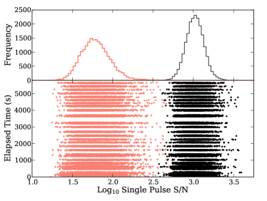
Figure 1: The S/N of our single-pulse observations. The peak S/N for a single phase bin appears to the left in salmon, while the total S/N summed over the onpulse region appears to the right in black. The bottom panel shows the time elapsed during the observation and missing intervals; the top panel shows the cumulative S/N distribution.

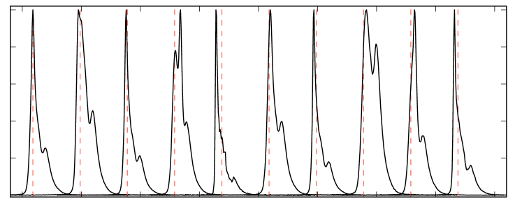
Figure 2: An example template basis. The leftmost basis function is constructed from pulses most resembling the mean, while the remainder are based on exceptional single pulses. The salmon, vertical dashed lines mark the same fiducial phase, viz. the maximum intensity in the mean profile. Several of the basis functions represent pulses with very bright sub-pulses at particular phases, while others capture unusual mixtures of components.

The precise topocentric pulsar frequency at the time of observation is unknown a priori. We measured it by extracting a TOA from each pulse and fitting a linear model. We computed the phase offset of each TOA to this linear model and then rotated the pulse profiles by this offset, equivalent to folding the data at the exact pulsar frequency. It is important that this phase alignment matches the true pulsar rotational phase with adequate precision. Because we have used more than $10^{4}$ pulses to estimate it, the phase alignment of any individual TOA will be better by a factor of 100 than the TOA measurement uncertainty. As we shall see below, this is adequate for our analysis.

We monitored the gain stability during the observation by analyzing the baseline (offpulse) noise in our single pulse profiles, dividing them into 276 (748) onpulse (offpulse) bins. The mean offpulse level drifted by about 5% over the observation, indicating the absolute gain was stable to at least this level. Indeed, it was likely more stable, as we found that the ratio of the mean to the standard deviation, which is linearly proportional to the system gain, $\kappa\equiv 4.2282(7)\times 10^{-3}$, did not vary over the observation. We thus expect S/N to be a good proxy for flux density. We note our observed $\kappa$ is also in agreement band-limited noise, viz. the radiometer relation, which predicts $\kappa=4.23\times 10^{-3}$ for 320 MHz of bandwidth.

The dual-band 10/50 cm (Granet et al., 2005) observing system we used has a system equivalent flux density (SEFD) of 25–30 Jy over the observing band, and the peak intensity of Vela reaches about 9 Jy (mean about 220 mJy). Thus, for a typical pulse, the system noise level is only increased by about 5% at peak, a negligible effect. However, peak intensity of the brightest pulses (giant micropulses, see Johnston et al., 2001) can be substantially brighter and exceed the SEFD, increasing the noise by more than 40%. We address this increased noise level further in §5.

Two important systematic effects could affect a single pulse analysis. First, broadband RFI can mimic sub-pulse structure. Such RFI is easily identified for PSR J0835$-$4510 by its lack of dispersion, and moreover is largely absent from the 10 cm band; we identified and discarded only four single pulses affected by impulsive RFI. Second, as the antenna tracks the source, the parallactic angle relative to the feed symmetry axis evolves, changing the illumination of the two feeds. Correcting such effects requires sophisticated modeling of the receiver response (e.g. van Straten, 2004, 2013). But, as the receiver is co-axial with little cross-polarization and the range of parallactic angles covered during the observation is small, we expect this effect to be minimal.

4 A ‘Pulse Shape’ Template Basis

Here, we discuss an approach for constructing a template basis based primarily on capturing the various observed pulse shapes. In §5.3, we discuss an approach based on the flux density of single pulses. In general, we expect any such a basis to only encapsulate a fraction of the true pulse-to-pulse variability. If single pulses are actually formed from random realizations of sub-pulses or ‘shots’ (Cordes, 1975; Hankins et al., 2003), there is no expectation that a family of single pulse shapes should emerge. Moreover, rare but bright pulses, such as the giant micropulses of PSR J0835$-$4510 or the true giant pulses of PSR B1937$+$21 (Cognard et al., 1996), substantially affect TOA measurements but cannot be faithfully represented by a small family of basis functions.

Nonetheless, the question is not one of perfection, but of efficacy, and below we show that a modest basis set can capture a substantial portion of single pulse variability.

4.1 Construction

An effective template basis is one that reproduces the pulse-to-pulse variation reasonably well without admitting too many degrees of freedom. In principle, for a fixed number of basis functions and a given set of single pulses, one could determine an optimal basis, i.e. one that minimizes the mean squared error between each single-pulse and the best-fitting basis function. However, this is an extremely challenging optimization problem!

Instead, we develop a basis iteratively. The initial basis comprises the mean template, and we begin by identifying the pulse least similar to the mean (see below). We then divide the single pulses into those more similar to the mean and those more similar to the outlier, and average those pulses to produce a basis with two templates. Next, we select the pulse least like either of these templates, re-classify the single pulses, produce a basis with three templates, and so on and so forth.

Generally, single pulse flux densities follow a lognormal distribution (Burke-Spolaor et al., 2012), while some pulsars displaying giant pulses and micropulses follow power law statistics, (see, e.g., Cairns, Johnston & Das, 2001; Cairns, 2004). To avoid constructing our basis from rare bright pulses, which would naturally be the strongest outliers due to their high S/N, we adopt a ‘reduced’ $\chi^{2}$,

$$\chi^{2}_{r}\equiv\sum_{i=1}^{N_{p}}(p_{i}-t_{i})^{2}/\sum_{i=1}^{N_{p}}p_{i}^{2},$$ (4)

which measures the distortion between the observed pulse shape and the template normalized to the S/N.

We note that this procedure does not necessarily converge to a unique basis. With each iteration, the basis functions are revised, and profiles ‘belonging’ to one basis function may be shuffled to others during the next classification. In practice, we find the the functions and classifications settle to a stable result after a few iterations.

To construct a mean pulse shape template, we co-added the first $10^{4}$ Vela pulses. We then applied the basis construction algorithm outlined here to the same pulses to compute template bases with varying numbers of basis functions. Templates from an example resulting basis appear in Figure 2.

4.2 Application and Efficacy

Here, we explore how well the basis encapsulates the pulse-to-pulse variability. First, we analyze the reduction in total mean squared error ($\chi^{2}$) of the set of single pulses relative to the mean template. For each pulse, we compute $\chi^{2}$ relative to either the mean template or the best-fitting basis template, and we then total the $\chi^{2}$ over all pulses. The results, shown in Fig. 3, indicate a dramatic improvement in $\chi^{2}$ with only a few basis functions. In fact, the total $\chi^{2}$ scales roughly as $N_{t}^{-1/4}$, though this relation is certainly coincidental and must steepen before $N_{t}$ becomes equal to the total number of single pulses!

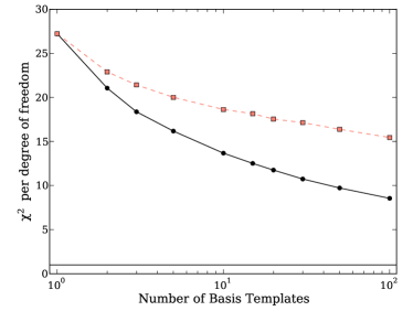
Figure 3: The total mean squared error ($\chi^{2}$), normalized by the total degrees of freedom, for the $10^{4}$ single pulses as a function of the number of functions in the template basis. The black solid line traces shows the ‘pulse shape’ basis (§4) and the $\chi^{2}$ scales approximately as $N_{t}^{-1/4}$. The salmon, dashed line shows the same trend for the ‘flux density’ basis of §5.3.

It is implicit in our definition of a single-pulse template basis that each pulse corresponds to one and only one basis function. We further make the assumption that pulses are uncorrelated. This is not true on short time-scales (a few pulses, Krishnamohan & Downs, 1983), but is a good assumption for longer intervals. (We discuss pulse-to-pulse correlation and its mitigation further in §6.) With these assumptions, it is straightforward to simulate pulse trains and compare these with observations. First, we classify the $10^{4}$ single pulses according to basis function by minimizing $\chi^{2}$. The fractions of pulses falling in each class are just the parameters of a multinomial distribution. Second, we have observed in our sample that that the distribution of pulse flux densities within each class is approximately described by a lognormal distribution. Thus, we realize $N$ simulated pulses by drawing an $N$-pulse sample from a multinomial distribution and then, for each classified pulse, drawing a flux from the appropriate lognormal distribution. An example train of 200 single pulses is shown alongside those taken from real data in Fig. 4.

Qualitatively, the simulations do a reasonable job of reproducing the observed pulse trains, though the real pulses show more stucture, particularly along the trailing edge of the peak. To quantify this, we have computed the modulation index (see Jenet, Anderson & Prince, 2001, for discussion), defined as $m=\sqrt{\sigma^{2}(\phi)-\sigma^{2}_{\mathrm{off}}}/\mu(\phi)$, i.e. the excess variance scaled to the mean intensity as a function of pulse phase. Figure 5 shows the results for single pulses: most of the modulation in the leading peak is captured, while variations are in the trailing region of the pulse in the real data are roughly twice those of the simulations. Much more interestingly, Figure 6 shows a similar factor of two deficit in simulation variability for 100-pulse sub-integrations. While some of this discrepancy results from failing to include self-noise in the simulations, the dominant effect must be pulse-to-pulse correlation, e.g. as observed by Krishnamohan & Downs (1983). On the other hand, we expect the simulations to become more faithful (approaching the single-pulse results) for longer sub-integrations.

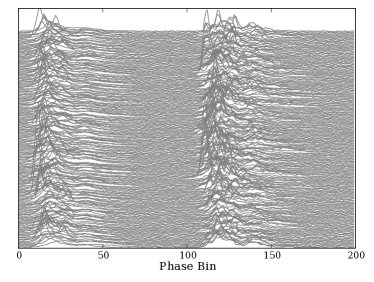
Figure 4: An example of 200 single pulses simulated as described in §4.2. Simulated pulses appear on the left, while 200 consecutive single pulses from PSR J0835$-$4510 appear to the right.

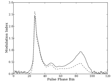
Figure 5: The phase-resolved modulation index (see main text) of the flux density of $10^{4}$ single pulses from simulations (dashed) and data (solid).

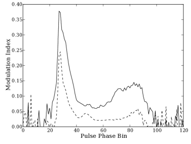
Figure 6: The phase-resolved modulation index of the flux density of 100 100-pulse sub-integrations from simulations (dashed) and data (solid).

5 Results

Here, we describe the application of three different timing algorithms and the ‘pulse shape’ basis. The first algorithm, ‘profiling’, does not require single pulse data, and we use it to introduce our analysis framework.

5.1 Applications without single pulse data – ‘P’

In the most common mode of pulsar observation, the pulsar signal time series is folded at the topocentric rotational frequency, producing a sub-integration containing many co-added single pulses. A typical integration time of 30 s records of order 100 pulses from a garden variety unrecycled pulsar. While the information contained in the single pulses is lost, we can still make inferences about the single pulse content of the sub-integration by estimating the coefficients of the basis template. Those inferences in turn can furnish improved constraints on the phase offset $\delta$. In terms of the basis function coefficients, the pdf for the sub-integration profile p becomes

$$f(\mathbf{p}\,|\,\delta,\mathbf{s},{\mathbf{b}},\mathbf{\sigma})=\prod_{i=1}^{N_{b}}\frac{1}{\sqrt{2\pi}\sigma_{i}}\exp\left[-\frac{1}{2}\left(\frac{p_{i}-(\mathbf{s}\cdot\mathbf{b})_{i}(\delta)}{\sigma_{i}}\right)^{2}\right].$$ (5)

For pulsar timing, the basis coefficients s are nuisance parameters. To maintain similarity with current pulsar timing techniques, we choose to use the profile likelihood to estimate $\delta$. That is, for each trial value of $\delta$, we determine the value of s that maximizes the likelihood, reducing the likelihood to a one-dimensional function $\mathcal{L}_{p}(\delta)$. Because s is formally positive semidefinite (no negative flux densities!), we restrict the optimization of s to positive values.

In the presentation below, we ignore the pulsar self-noise contribution and assume a constant $\sigma$. We repeated our analysis including self-noise in the model, but found negligible changes to the measurements of $\delta$ and its uncertainty. That is, for Vela, the self-noise effect is small compared to pulse-to-pulse variability. As introducing the self-noise (heteroscedasticity) substantially complicates the computation for little gain, we neglect it henceforth.

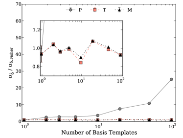
Figure 7: The precision of the phase measurement $\delta$ as a function of the complexity of the basis for three different realizations of the likelihood, using 100-pulse sub-integrations of simulated data. The grey, solid trace (‘P’) corresponds to the profile method, discussed in §5.1. The dashed salmon and dot-dashed black lines correspond to the ‘tagging’ methods discussed in §5.2, both without (‘T’) and with (‘M’) the addition of the multinomial likelihood. All results are scaled to the ideal measurement precision (see main text). The inset is as the main figure, but zoomed to show that the tagging methods perform optimally, reaching the Fisher precision. In these results, the abscissa indicates $N_{b}$ for both the simulations and the fitting, i.e. as if one had perfect knowledge of the family of single pulse variations. Finally, note that the error bars due to finite sample size are shown for the $N_{b}=1$ and suppressed for the remainder; see main text for details.

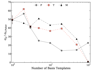
Figure 8: As Fig. 7, but the simulations use an $N_{b}=100$ basis while the abscissa indicates the $N_{b}$ used in the fits. This case corresponds to imperfect knowledge of the panoply of pulse shapes.

5.1.1 Simulations

To validate and characterize the approach under controlled but realistic conditions, we simulated pulse trains from the basis as described in §4.2 and then synthesized sub-integrations with 100, 200, and 400 pulses. These lengths, and the number of simulated sub-integrations, are chosen to match those of the data, described below.

For each sub-integration, we maximized the likelihood of equation 5 to determine the phase shift estimator $\hat{\delta}$. We then computed the standard deviation of $\hat{\delta}$ over the set of simulations and normalized it to the idealized scatter, i.e. what we would observe in the absence of jitter/SWIMS and self-noise. This uncertainty is given by the Fisher information of the mean template, which gives a lower limit for the variance for $\hat{\delta}$,

$$\sigma^{-2}_{\hat{\delta},\mathrm{Fisher}}=\sum_{i}\left(\frac{1}{\sigma_{r}}\frac{\partial t_{i}}{\partial\delta}\right)^{2},$$ (6)

where $\sigma_{r}$ is again the radiometer noise.

In our simulations, we can choose to simulate profiles with a basis with the same $N_{b}$ we use to maximize the likelihood, or we can fix it at some representative $N_{b}$. The former essentially validates the method, while the latter probes how the results change when the basis and the data disagree, as will certainly be the case for real data. Accordingly, we follow both approaches.

The results for which $N_{b}$ is the same for both simulations and fitting appear in the grey traces labelled ‘P’ in Fig. 7. Here, for clarity, we show the results for the 100-pulse sub-integrations; the 200-pulse and 400-pulse results are similar. The leftmost values, corresponding to a template basis with $N_{b}=1$, i.e. the mean template or ‘traditional’ pulsar timing, shows a scatter consistent with the Fisher limit—certainly to be expected, since simulations from a template with $N_{b}=1$ have no jitter/SWIMS. Since the set of simulations changes for each $N_{b}$, the data are uncorrelated; this will not be the case for scenarios described below. As the complexity of the simulations increases, we see the profile method slowly diverges as the degrees of freedom increase. Thus, we expect the method may ultimately break down if we attempt to fit a pulsar with very complicated pulse-to-pulse variability.

In the second set of simulations, we fix $N_{b}=100$ for a high level of pulse-to-pulse variability, and we then vary $N_{b}$ in our fits of $\hat{\delta}$. Now, the $N_{b}=1$ case shows a jitter/SWIMS level of about 50 times the radiometer limit, consistent with our observation that our simulations produce about half of the pulse-to-pulse variability of the actual data. As we increase $N_{b}$, the profile method is able to successfully reconstruct some of the single pulse variability, reducing the jitter/SWIMS level by a factor of three for $N_{b}=20$, before slowly diverging. Since we use the same set of simulations for each value of $N_{b}$ on the abscissa, these points are correlated, and the error bars should be interpreted as uncertainty on overall amplitude rather than as a measure of scatter.

Thus, we conclude that this ‘profile’ method is quite effective in removing jitter/SWIMS noise under the idealized conditions of our assumptions about single pulse variability. This approach should be especially effective for pulsars with less complicated pulse-to-pulse variability, and for those whose single pulses are too faint for effective single pulse ‘tagging’ (see below), such as MSPs.

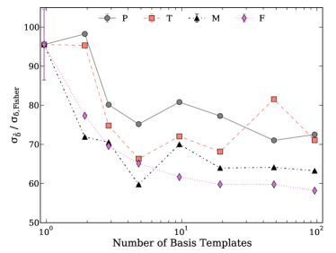
Figure 9: As Fig. 7, but for data from PSR J0835$-$4510. Additionally, the orchid, dotted trace shows the results for the flux-tagging scheme described in §5.3.

5.1.2 Data

We now apply the profile method to synthesized sub-integrations of varying lengths from the data set described above. After excising the $10^{4}$ pulses used to build the basis template and those affected by RFI, 11,182 pulses remain. Maintaining a sufficiently large sample of sub-integrations to measure the scatter of $\hat{\delta}$ imposes a limit on sub-integration length of about 400 pulses, or 36 s, typical of a fold-mode sub-integration. However, as we discuss below, we expect the results to scale to longer integrations, and perhaps to improve as correlations between single pulses become less important.

As with the simulations, for each synthesized sub-integration, we maximized $\mathcal{L}_{p}(\delta)$ to determine $\hat{\delta}$ and examined the distribution of values. The results are summarized in Fig. 9. As before, the leftmost points correspond to ‘traditional’ pulsar timing and show the jitter/SWIMS level is about 100 times the ideal limit. As with the second set of simulations, because the same data set is used for each set of basis templates, the results are correlated.

As we might expect from the failure of our basis to reproduce the lion’s share of the pulse-to-pulse variability, the reduction in scatter in moving to $N_{b}>1$ is substantially poorer than in simulations. Nonetheless, we see a gradual impovement in the level of scatter, as the basis complexity increases and captures more of the pulse-to-pulse variability, with a typical scatter reduction of about 25%. We also note that longer sub-integrations show a lower level of jitter/SWIMS relative to the ideal (which scales as $1/\sqrt{t}$) than shorter sub-integrations, suggesting that performance does indeed improve as the pulse-to-pulse correlation time-scale becomes short compared to the sub-integration length.

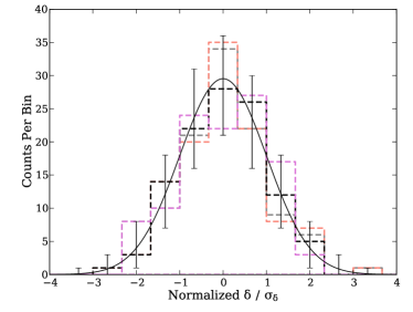
Figure 10: The distribution of the error-normalized residuals after normalization by the sample standard deviation, for all three ‘shape’ algorithms, with 100-pulse sub-integrations and $N_{b}=20$. The black trace and error bars show the expected gaussian distribution and the range covered by 90% of random realizations of identical histograms of gaussian random variables. The colors follow the convention of Fig. 7. The orchid line shows the same result for the ‘flux basis’ of §5.3.

While a reduction in the scatter of measured phase offsets clearly improves precision, an accurate estimate of the remaining noise is of vital importance for pulsar timing. Ideally, reliable error estimates can be extracted directly from the timing procedure, and we expect this could be achieved even without a perfect template basis via bootstrap methods. But minimally, all we require is that the normalized residuals follow a gaussian distribution. These normalized residuals appear in Fig. 10, showing that the estimators for $\hat{\delta}$ do indeed follow a normal distribution.

5.2 Applications with single pulse data – ‘T’ and ‘M’

Next, we consider a hybrid mode of observation—one in which we produce sub-integrations as before, but in which we also have access to single pulse data. While many avenues are available, including marginalization over template classification and Monte Carlo Markov chain methods, we opt for a simple approach that might more readily be implemented in an online pulsar data recorder. Because nearly every pulse in our data set has a high S/N, it can be uniquely associated with a single basis function. This leads to the idea of ‘pulse tagging’—each incoming single pulse is classified and its flux (scale parameter) measured; the pulse itself can then be discarded. The classifications and scales are then used to build an optimized template from the template basis, which is in turn used to measure the phase offset of the full sub-integration. A key point: we are not “using the data to fit the data”. Because we do not know the correct phase offset $\delta$ a priori, we perform classification and template construction over a range of values of $\delta$. This process is similar to constructing a profile likelihood, in which we optimize for the (discrete) profile classification parameters.

5.2.1 Simulations

As before, we test this method with simulated data. In the first ‘sanity check’ approach, we see that the approach performs flawlessly. That is, by tagging the individual pulses, we are able to construct a template for each sub-integration that entirely accounts for jitter/SWIMS, and we reach the Fisher limit for estimator uncertainty. Importantly, despite implicitly fitting for the profile class and scale of each pulse, we see no evidence for overfitting.

The second set of simulations, in which all simulated profiles are drawn from a $N_{b}=100$ template basis, are more interesting. For fits with $N_{b}\ll 100$, there is no improvement in jitter/SWIMS level. But once we reach $N_{b}=50$, jitter/SWIMS is reduced by roughly half, and as in the first set of simulations we remove jitter/SWIMS entirely once $N_{b}$ is consistent between simulation and fit. This result is readily explained. For the $N_{b}\ll 100$ cases, no template basis function maps well onto a single pulse, and tagging process will essentially build up the mean template. On the other hand, once the basis begins to encapsulate single pulses, we achieve a template that accurately records the influence of pulse-to-pulse variability.

From these results, we conclude that the single pulse tagging approach is extremely effective (entirely removing jitter/SWIMS) if the template basis is well-suited to the data.

5.2.2 Data

The results of applying this approach to our test data set appear in the salmon traces of Fig. 9. Jitter/SWIMS decreases rapidly with increasing $N_{b}$ through $N_{b}=5$, before saturating at roughly 65% of the $N_{b}=1$ level. These results are largely consistent with our understanding that the template basis should be well matched to single pulse variability. As we saw in Fig. 3, we capture most of the pulse-to-pulse variability that we can with relatively few template basis functions, and increasing $N_{b}$ beyond about 5 yields only slow gain.

Although the tagging method seems effective in simulations, there is in principle additional information we can apply to the fits that may better handle real data. E.g., very rare, bright pulses can substantially affect a TOA measurement (Osłowski et al., 2014), so they must be represented in an effective template basis. On the other, less intense pulses with morphology similar to giant pulses should not be so classified. Put another way, the pulse counts and flux densities associated with each basis are random variables, and we can add terms reflecting this to the likelihood. Substantial misclassification will then be penalized. As discussed in §4.1, we can easily determine the expected rates of pulses associated with each basis, as well as measure their flux distribution. With our neglect of pulse-to-pulse correlation, these terms enter the likelihood multiplicatively through the multinomial distribution (for the classes) and $N_{p}$ lognormal distributions (for the fluxes). Suppressing constant terms, this log likelihood is

$$\begin{split}\log\mathcal{L}=&-\frac{1}{2}\sum_{i=1}^{N_{p}}\left[p_{i}-t_{i}(\delta)\right]^{2}+\left[\frac{\log s_{i}-\mu_{b}}{\sigma_{b}}\right]^{2}+2\log s_{i}\\ &+\sum_{i=1}^{N_{b}}\left[n_{i}\log a_{i}-\log n_{i}!\right],\end{split}$$ (7)

where

$$\mathbf{t}=\sum_{i=1}^{N_{p}}s_{i}\mathbf{b}_{i},$$ (8)

$\mathbf{b}_{i}$ is the best-fit basis for the $i$th pulse, and $s_{i}$ is the corresponding best-fit flux. The $a_{i}$ are the parameters of the multinomial distribution (relative pulse frequency for each basis) and the $n_{i}$ are the number of pulses tagged into each basis.

In our data—and in any data in which jitter/SWIMS is important—the ‘$\chi^{2}$’ term in equation 7 utterly dominates the multinomial and lognormal terms, and the relative weighting must be adjusted to allow the latter data to provide constraints. There are two ‘natural’ approaches, and we find they yield similar results: (1) re-scale the $\chi^{2}$ term such that the residual $\chi^{2}$ per degree of freedom is unity or (2) re-scale the $\chi^{2}$ such that the $\chi^{2}$ term contributes equally to the total likelihood. We adopt the latter approach.

Applying these additional constraints yields a small decrease in the scatter of our sample, in some cases reducing the jitter noise by as much as 40%; see the black traces of Fig. 9.

5.3 A Flux Basis

The previous methods have all focussed on pulse shape rather than information encoded in the pulse profile normalization, i.e. its flux density. However, for PSR J0835$-$4510, there is a additionally a strong correlation between the peak intensity of a pulse and the phase at which that peak falls (Krishnamohan & Downs, 1983), and strong pulses have a large influence on TOA estimation. We thus consider here a ‘flux basis’ and investigate its performance relative to the ‘shape basis’.

We construct this basis by simply computing the peak S/N in each single pulse, dividing the pulses into bins logarithmically uniform in peak S/N, and constructing templates from the average pulse shape in each bin. To perform timing on a synthesized sub-integration, we assume as in §5.2 that we can measure single pulse properties, specifically the peak S/N in each single pulse, selecting the basis template from the matching S/N bin, and adding up the matched templates. The resulting template naturally reflects the outsized contribution of strong fluxes to a sub-integration. Note that it also establishes the additional observational requirement of stable gain/flux calibration.

The results are extremely interesting. In Figure 3, we note that the flux basis captures less of the pulse-to-pulse variability. The timing performance, however, is excellent. The results appear as the orchid-coloured trace labelled ‘F’ in Figure 9, showing a performance that is generally the best of the methods explored here, offering a robust 40% improvement over the jitter/SWIMS noise level!

The root of this discrepancy between superiour timing performance and poor pulse-shape reproduction offers some insight into the Vela’s pulse emission process. Aside from the clear flux/phase correlation, it is evident that the emission mechanism can produce pulses with similar shapes at different observed phases, which in turn may point to propagation effects as an important source of jitter/SWIMS. Whether similar effects are common in other pulsars, and how they might be explored (e.g. through polarimetry) are interesting topics for future work and we discuss them further below.

6 Summary and Future Work

We have presented a new method for pulsar timing using single-pulse based likelihood. In simulations, we showed these methods are capable of materially reducing or entirely eliminating the jitter/SWIMS noise associated with pulse-to-pulse variability. We demonstrated less dramatic but nonetheless substantial reductions in the jitter/SWIM noise of data from the bright Vela pulsar.

Our results are encouraging and motivate future work. In particular, much could be done simply be expanding the scope of the data used to build the basis function. Our ‘training set’ of pulses for Vela was limited to a mere $10^{4}$ single pulses, comparable in size to the set of pulses we could use to test the algorithms. It must necessarily have missed rare pulses, and the limited number of basis function likely forces the combination of similar but distinct pulse classes into a single template. Indeed, our simulations, in which we had perfect control over the complexity of pulse-to-pulse variability, showed that we required a basis with nearly the full complexity of the simulations to fully remove jitter/SWIMS (Figure 7).

Moreover, Vela exhibits pulse-to-pulse correlation, contrary our simplifying assumption of independent pulses. Though more complicated computationally, a ‘two-pulse’ template basis—whose members are two consecutive single pulses—is straightforward conceptually and could capture much of the observed single pulse correlation. Extension to ‘N-pulse’ bases would help even more. Both cases would require more extensive training sets. Likewise, it is straightforward to extend these methods to pulsars with periodic sub-pulse modulation, in which case the natural unit of a basis is the modulation period.

In general, it seems likely that per-pulsar tuning will be required to find the best combination of template basis and fitting method. For Vela, an optimal method must clearly take advantage of the TOA / flux density correlation. In the case of PSR J0437$-$4715, Osłowski et al. (2013) observed a correlation between the phase centroid and the pulse polarization, suggesting an optimal template basis for thise pulsar must include polarimetry. For mode changing pulsars, a separate template basis for each mode could be determined, and subsequent application of the timing algorithms would furnish both correct TOAs and an automatic classification of the pulsar modes.

While there is much future work to be done, a pressing question remains: if the current template basis can do a good job of describing single-pulse variation (Figure 3), why is the timing only modestly improved? This ultimately boils down to the still poorly understood phenomenology of single pulse variability. For pulsars whose emission truly comprises ‘shots’ of emission within a guiding envlope (Cordes, 1975), fully modelling the covariance à la Osłowski et al. (2011) is the optimal approach. Whereas pulsars which demonstrate at least some underlying pattern, in which similar single pulses appear repeatedly over time, will benefit from the recovery of additional information by the deterministic approach advocated here. Though the pulse-to-pulse correlation observed for PSR J0835$-$4510 implies at least some repetition, it may yet be that the single pulses also possess an irreducible random component. In this case, the reduction of jitter/SWIMS by 30–40% achieved here may be the best possible, and the rest that can be done is accurately estimate uncertainties. Indeed, improving the timing algorithms in the ways outlined above will provide a stringent test of the true randomness of the pulsar mechanism, and it is thus of keen interest to collect single pulses from a large set of bright pulsars for further study.

What would be required to implement this method in a practical pulsar timing programme? As we have discussed, a sina qua non is a large training set of high-quality single pulses. These can be obtained in a single dedicated session, possibly on a target-of-opportunity basis when a pulsar is unusually bright due to scintillation. Subsequent observations should record single pulses, but possibly with reduced quality. Compared to typical folded sub-integrations, full-resolution single pulse data from young (millisecond) pulsars requires about 100 (10,000) times more storage. While full-resolution data is intrinsically interesting for studying the pulsar mechanism, our method is based on fully reduced (in frequency and polarization) data, and recording such archives requires only modest additional storage. We strongly advocate such a commensal programme, as it will both enable our proposed study of jitter/SWIMS and help inform the design of future pulsar timing instrumentation.

References

- Antoniadis et al. (2013) Antoniadis J. et al., 2013, Science, 340, 448
- Burke-Spolaor et al. (2012) Burke-Spolaor S. et al., 2012, MNRAS, 423, 1351
- Cairns (2004) Cairns I. H., 2004, ApJ, 610, 948
- Cairns, Johnston & Das (2001) Cairns I. H., Johnston S., Das P., 2001, ApJ, 563, L65
- Cognard et al. (1996) Cognard I., Shrauner J. A., Taylor J. H., Thorsett S. E., 1996, ApJ, 457, L81
- Cordes (1975) Cordes J. M., 1975, PhD thesis, California Univ., San Diego.
- Demorest et al. (2013) Demorest P. B. et al., 2013, ApJ, 762, 94
- Demorest et al. (2010) Demorest P. B., Pennucci T., Ransom S. M., Roberts M. S. E., Hessels J. W. T., 2010, Nature, 467, 1081
- Granet et al. (2005) Granet C. et al., 2005, IEEE Antennas Propagation Magazine, 47, 13
- Gwinn & Johnson (2011) Gwinn C. R., Johnson M. D., 2011, ApJ, 733, 51
- Hankins et al. (2003) Hankins T. H., Kern J. S., Weatherall J. C., Eilek J. A., 2003, Nature, 422, 141
- Hermsen et al. (2013) Hermsen W. et al., 2013, Science, 339, 436
- Hewish et al. (1968) Hewish A., Bell S. J., Pilkington J. D. H., Scott P. F., Collins R. A., 1968, Nature, 217, 709
- Hobbs et al. (2014) Hobbs G., Dai S., Manchester R. N., Shannon R. M., Kerr M., Lee K. J., Xu R., 2014, ArXiv e-prints
- Hobbs, Lyne & Kramer (2010) Hobbs G., Lyne A. G., Kramer M., 2010, MNRAS, 402, 1027
- Jenet, Anderson & Prince (2001) Jenet F. A., Anderson S. B., Prince T. A., 2001, ApJ, 546, 394
- Johnston et al. (2001) Johnston S., van Straten W., Kramer M., Bailes M., 2001, ApJ, 549, L101
- Kaspi, Taylor & Ryba (1994) Kaspi V. M., Taylor J. H., Ryba M. F., 1994, ApJ, 428, 713
- Keith et al. (2013) Keith M. J. et al., 2013, MNRAS, 429, 2161
- Kramer et al. (2006) Kramer M., Lyne A. G., O’Brien J. T., Jordan C. A., Lorimer D. R., 2006, Science, 312, 549
- Kramer & Wex (2009) Kramer M., Wex N., 2009, Classical and Quantum Gravity, 26, 073001
- Krishnamohan & Downs (1983) Krishnamohan S., Downs G. S., 1983, ApJ, 265, 372
- Kulkarni (1989) Kulkarni S. R., 1989, AJ, 98, 1112
- Lattimer & Prakash (2004) Lattimer J. M., Prakash M., 2004, Science, 304, 536
- Lyne et al. (2010) Lyne A., Hobbs G., Kramer M., Stairs I., Stappers B., 2010, Science, 329, 408
- Manchester et al. (2013) Manchester R. N. et al., 2013, PASA, 30, 17
- Osłowski et al. (2014) Osłowski S., van Straten W., Bailes M., Jameson A., Hobbs G., 2014, MNRAS, 441, 3148
- Osłowski et al. (2013) Osłowski S., van Straten W., Demorest P., Bailes M., 2013, MNRAS, 430, 416
- Osłowski et al. (2011) Osłowski S., van Straten W., Hobbs G. B., Bailes M., Demorest P., 2011, MNRAS, 418, 1258
- Ransom et al. (2014) Ransom S. M. et al., 2014, Nature, 505, 520
- Rickett (1975) Rickett B. J., 1975, ApJ, 197, 185
- Shannon & Cordes (2010) Shannon R. M., Cordes J. M., 2010, ApJ, 725, 1607
- Shannon, Osłowski & et al. (2014) Shannon R. M., Osłowski, Dai S., et al., 2014, ArXiv e-prints
- Shannon et al. (2013) Shannon R. M. et al., 2013, Science, 342, 334
- Taylor (1992) Taylor J. H., 1992, Royal Society of London Philosophical Transactions Series A, 341, 117
- Taylor, Fowler & McCulloch (1979) Taylor J. H., Fowler L. A., McCulloch P. M., 1979, Nature, 277, 437
- van Straten (2004) van Straten W., 2004, ApJS, 152, 129
- van Straten (2013) van Straten W., 2013, ApJS, 204, 13
- van Straten & Bailes (2011) van Straten W., Bailes M., 2011, PASA, 28, 1
- Yardley et al. (2011) Yardley D. R. B. et al., 2011, MNRAS, 414, 1777
Acknowledgments
We are grateful to Stefan Osłowski for input on an early draft and to the anonymous referee for helpful criticism that improved the paper. The Parkes radio telescope is part of the Australia Telescope, which is funded by the Commonwealth Government for operation as a National Facility managed by CSIRO.