Efficient Quantum Compression for Ensembles of Identically Prepared Mixed States

Abstract

We present one-shot compression protocols that optimally encode ensembles of $N$ identically prepared mixed states into $O(\log N)$ qubits. In contrast to the case of pure-state ensembles, we find that the number of encoding qubits drops down discontinuously as soon as a nonzero error is tolerated and the spectrum of the states is known with sufficient precision. For qubit ensembles, this feature leads to a 25% saving of memory space. Our compression protocols can be implemented efficiently on a quantum computer.

Storing data into the smallest possible space is of crucial importance in present-day digital technology, especially when dealing with large amounts of information and with limited memory space Sagiroglu and Sinanc (2013). The need for saving space is even more pressing in the quantum domain, where storing data is an expensive task that requires sophisticated error correction techniques Julsgaard et al. (2004); Zhao et al. (2009); Biercuk et al. (2009).

For quantum data, Schumacher’s compression Schumacher (1995) and its extensions Jozsa and Schumacher (1994); Lo (1995); Horodecki (1998); Jozsa et al. (1998); Bennett et al. (2006) provide optimal ways to store information in the asymptotic limit of many identical and independent uses of the same source. However, in many situations there may be correlations from one use of the source to the next. In such situations, it is convenient to regard $N$ uses of the original source as a single use of a new source, which emits messages of length $N$. This scenario is an instance of one-shot quantum data compression Datta et al. (2013). An important example of one-shot compression is when the states emitted at $N$ subsequent moments of time are perfectly correlated, resulting in codewords of the form $\rho_{x}^{\otimes N}$ for some density matrix $\rho_{x}$ and some random parameter $x$. This situation arises when the original source is an uncharacterized preparation device, which generates the same quantum state at every use. For quantum bits (qubits), Plesch and Bužek Plesch and Bužek (2010) observed that every ensemble of identically prepared pure states can be stored without any error into $\log(N+1)$ qubits, thus allowing for an exponential saving of memory space. Recently, Rozema et al Rozema et al. (2014) brought this idea into the realm of experiment, demonstrating a prototype of one-shot compression in a photonic setup.

The possibility of implementing one-shot compression in the lab opens new questions that require one to go beyond the ideal case of pure states and no errors. First, due to the presence of noise, real-life implementations typically involve mixed states—think,  e. g.,  of quantum information processing with NMR Vandersypen and Chuang (2005), where the standard is to have thermal states at a given temperature, or, more generally, of mixed-state quantum computing Aharonov et al. (1998); Knill and Laflamme (1998); Shor and Jordan (2008); Datta et al. (2008); Lanyon et al. (2008). For mixed states, the basic principle of pure-state compression does not work: in the qubit case, for example, projecting the quantum state into the smallest subspace containing the code words does not lead to any compression if the states $\rho_{x}^{\otimes N}$ are mixed, because in that case the smallest subspace is the whole Hilbert space. As a result, it is natural to search for compression protocols that work for mixed states and to ask which protocols achieve the best compression performance. An even more important question is how the number of qubits needed to store data depends on the errors in the decoding. Tolerating a nonzero error is natural in real-life implementations, which typically suffer from noise and imperfections.

In this Letter we answer the above questions, proposing compression protocols for ensembles of identically prepared mixed states. We first analyze the zero-error scenario, showing that the storage of $N$ mixed qubits with known purity and unknown Bloch vector requires a quantum memory of at least $2\log N$ qubits. The size of the required memory is twice that of the required memory for pure states, but it is still exponentially smaller that the initial data size. The maximum compression is achieved by a protocol that does not require knowledge of the purity. We then investigate the more realistic case of protocols with an error tolerance. When the purity is known with sufficient precision, we find out that tolerating an error, no matter how small, allows one to encode the initial data into only $3/2\,\log N$ qubits, plus a small correction independent of $N$. Remarkably, the discontinuity in the error parameter takes place as soon as the prior knowledge of the purity is more precise than the knowledge that could be gained by measuring the $N$ input qubits. The existence of a discontinuity is a striking deviation from the pure-state case, for which we prove that there is no significant advantage in introducing an error tolerance. Furthermore, we show that our compression protocol can be implemented efficiently and that the compression rate is optimal under the requirements that the encoding be rotationally covariant and the decoding preserve the magnitude of the total angular momentum. These assumptions are relevant in physical situations where the mixed states are used as indicators of spatial directions Demkowicz-Dobrzański (2005); Bagan et al. (2000) and the decoding operations are limited by conservation laws Gour and Spekkens (2008); Marvian and Spekkens (2013, 2014a, 2012); Ahmadi et al. (2013); Marvian and Spekkens (2014b). All our results can be generalized to quantum systems of arbitrary finite dimension, where we quantify how the presence of degeneracy in the spectrum affects the compression rates.

Let us start from the qubit case, assuming $N$ to be even for the sake of concreteness. We denote by $\mathcal{E}:\mathcal{H}^{\otimes N}\to\mathcal{H}_{\rm enc}$ ($\mathcal{D}:\mathcal{H}_{\rm enc}\to\mathcal{H}^{\otimes N})$ the encoding (decoding) channel, where $\mathcal{H}$ is the Hilbert space of a single qubit and $\mathcal{H}_{\rm enc}$ is the Hilbert space of the encoding system. For an ensemble of identically prepared qubit states $\{\rho^{\otimes N}_{x}\,,p_{x}\}$ the average error of the compression protocol is

$$e_{N}=\sum_{x}\,p_{x}\frac{\left\|\rho^{\otimes N}_{x}-\mathcal{D}\circ\mathcal{E}\left(\rho_{x}^{\otimes N}\right)\right\|}{2}\,,$$ (1)

$\|A\|$ denoting the trace norm. We consider ensembles where all the states $\rho_{x}$ have the same purity, which is assumed to be perfectly known (this assumption will be lifted later). Let us write $\rho_{x}$ as $\rho_{\mathbf{n}}=p\,|\mathbf{n}\rangle\langle\mathbf{n}|\,+(1-p)\,|-\mathbf{n}\rangle\langle-\mathbf{n}|$, where $|\mathbf{n}\rangle$ denotes the two-dimensional pure state with Bloch vector $\mathbf{n}=(n_{x},n_{y},n_{z})$ and $p\geq 1/2$ is the maximum eigenvalue. We focus on mixed states $(p\not=1)$, excluding the trivial case $p=1/2$, in which the ensemble consists of just one state. For $p\not\in\{1,1/2\}$, we call the ensemble $\{\rho_{\mathbf{n}}^{\otimes N}\,,p_{\mathbf{n}}\}$ complete if the probability distribution $p_{\mathbf{n}}$ is dense in the unit sphere. The typical example is an ensemble of mixed states with known purity and completely unknown Bloch vector. For every complete ensemble we demonstrate a sharp contrast between two types of compression: (i) zero-error compression, wherein the decoded state is equal to the initial state, and (ii) approximate compression, wherein small errors are tolerated. In the zero-error case we have the following

Theorem 1.

The minimum number of logical qubits needed to compress a complete $N$-qubit ensemble is $\lceil 2\log(N+2)-2\rceil$. Every compression protocol that has zero error on a complete ensemble must have zero error on every ensemble of identically prepared mixed states and on every ensemble of permutationally invariant N-qubit states.

Intuitively, the reason for the exponential reduction of the number of qubits is that the states in the ensemble are invariant under permutations and, therefore, they do not carry all the information that could be encoded into $N$ qubits. This observation was anticipated by Blume-Kohout et al in the context of state discrimination and tomography Blume-Kohout et al. (2012). The key point of Theorem 1 is the optimality proof, which establishes that if a mixed-state ensemble is complete, then compressing it is as hard as compressing any arbitrary ensemble of permutationally invariant states sup .

In preparation of our analysis of approximate compression, it is instructive to look into an optimal protocol achieving zero-error compression. The starting point is the Schur-Weyl duality Fulton and Harris (1991), stating that there exists a basis in which the $N$-fold tensor action of the group $\mathsf{GL}(2)$ and the natural action of the permutation group $S_{N}$ are both block diagonal. In this basis, the Hilbert space of the $N$ qubits can be decomposed as

$$\mathcal{H}^{\otimes N}\simeq\bigoplus_{j=0}^{N/2}\left(\mathcal{R}_{j}\otimes\mathcal{M}_{j}\right),$$ (2)

where $j$ is the quantum number of the total angular momentum, $\mathcal{R}_{j}$ is a representation space, in which the group $\mathsf{GL}(2)$ acts irreducibly, and $\mathcal{M}_{j}$ is a multiplicity space, in which the group acts trivially. Now, since the state $\rho_{\mathbf{n}}^{\otimes N}$ is invariant under permutations of the $N$ qubits, one has

$$\rho_{\mathbf{n}}^{\otimes N}=\bigoplus_{j=0}^{N/2}\,q_{j,N}\,\left(\rho_{\mathbf{n},j}\otimes\frac{I_{m_{j}}}{m_{j}}\right),$$ (3)

where $q_{j,N}$ is a suitable probability distribution in $j$, $\rho_{\mathbf{n},j}$ is a quantum state on $\mathcal{R}_{j}$, $I_{m_{j}}$ is the identity on $\mathcal{M}_{j}$, and $m_{j}$ is the dimension of $\mathcal{M}_{j}$. From Eq. (3) it is obvious that all information about the input state lies in the representation spaces. Hence, $\rho_{\mathbf{n}}^{\otimes N}$ can be encoded faithfully into the state $\mathcal{E}\left(\rho_{\mathbf{n}}^{\otimes N}\right)=\bigoplus_{j}q_{j,N}\,\rho_{\mathbf{n},j}$. Such state has an exponentially smaller support, contained in the space $\mathcal{H}_{N}:=\bigoplus_{j=0}^{N/2}\mathcal{R}_{j}$, whose dimension is $\dim\mathcal{H}_{N}=\left(N/2+1\right)^{2}$. Hence, the initial state can be encoded into $\lceil\log\dim\mathcal{H}_{N}\rceil$ qubits—the amount declared in Theorem 1. A perfect decoding is achieved by the channel

$$\mathcal{D}(\rho):=\bigoplus_{j}\,\left(P_{j}\,\rho\,P_{j}\otimes\frac{I_{m_{j}}}{m_{j}}\right)\,,$$ (4)

where $P_{j}$ is the projector on the representation space $\mathcal{R}_{j}$.

Considering that qubits are a costly resource, it is worth pointing out a slight modification of the above protocol, which uses approximately $\log N$ qubits and $\log N$ classical bits. The modified protocol consists in (i) measuring the value of $j$, thus projecting $N$ qubits into the state $\rho_{\mathbf{n},j}\otimes I_{m_{j}}/m_{j}$, (ii) discarding the multiplicity part, (iii) encoding the state $\rho_{\mathbf{n},j}$ into $\lceil\log(N+1)\rceil$ qubits, and (iv) transmitting the encoded state to the receiver, along with a classical message specifying the value of $j$. Knowing the value of $j$, the receiver can append an additional system in the state $I_{m_{j}}/{m_{j}}$ and embed the state $\rho_{\mathbf{n},j}\otimes I_{m_{j}}/m_{j}$ into the right subspace.

Let us consider now the more realistic case of approximate compression. Here, the number of encoding qubits drops down discontinuously.

Theorem 2.

For every allowed error rate $\epsilon>0$ and for every complete qubit ensemble, there exists a number $N_{0}>0$ such that for any $N\geq N_{0}$ the ensemble can be encoded into $3/2\log N+\log[4(2p-1)\sqrt{\ln(2/\epsilon)}]$ qubits with error smaller than $\epsilon$.

The idea is to work out the explicit form of the probability distribution $q_{j,N}$ in Eq. (3), given by

$$q_{j,N}=\frac{2j+1}{2j_{0}} \left[B\left(N+1,p,\frac{N}{2}+j+1\right)\right.$$

$$\left.~{}-B\left(N+1,p,\frac{N}{2}-j\right)\right]$$ (5)

where $B(n,p,k)$ is the binomial distribution with $n$ trials and with probability $p$, and $j_{0}=(p-1/2)(N+1)$. For large $N$, the distribution $q_{j,N}$ is approximately the product of a linear function with the normal distribution of variance $(N+1)p(1-p)$ centered around $j_{0}$. In order to compress, we get rid of the tails: for every $\epsilon>0$, we select a set $\mathsf{S}_{\epsilon}:=\left\{j_{0}-\lfloor\sqrt{\ln(2/\epsilon)N}\rfloor,\dots,j_{0}+\lfloor\sqrt{\ln(2/\epsilon)N}\rfloor\right\}$ and we compress the state $\rho_{\mathbf{n}}^{\otimes N}$ into the encoding space $\mathcal{H}_{\rm enc}=\bigoplus_{j\in\mathsf{S}_{\epsilon}}\mathcal{R}_{j}$, by applying the quantum channel

$$\mathcal{E}(\rho):=\bigoplus_{j\in\mathsf{S}_{\epsilon}}\,\operatorname{Tr}_{\mathcal{M}_{j}}\,\left[\,\Pi_{j}\,\rho\,\Pi_{j}\,\right]+\sum_{j\not\in\mathsf{S}_{\epsilon}}\,\operatorname{Tr}\left[\Pi_{j}\,\rho\right]\,\rho_{0}\,,$$ (6)

where $\Pi_{j}$ is the projector on $\mathcal{R}_{j}\otimes\mathcal{M}_{j}$, $\operatorname{Tr}_{\mathcal{M}_{j}}$ is the partial trace over $\mathcal{M}_{j}$, and $\rho_{0}$ is a fixed state with support inside $\mathcal{H}_{\rm enc}$. The encoding space has dimension

$$\dim\mathcal{H}_{\rm enc} =\sum_{j\in\mathsf{S}_{\epsilon}}\,(2j+1)\leq\,(2j_{0}+1)\left(2\sqrt{N\ln\frac{2}{\epsilon}}+1\right)\,,$$

growing as $N^{3/2}$. The initial state can be recovered, up to error $\epsilon$, by a suitable decoding channel sup .

Theorem 2 guarantees that $N$ identical copies of a mixed state with known purity can be stored faithfully to $\epsilon$ into $3/2\log N$ qubits, plus an overhead that is doubly logarithmic in $1/\epsilon$. This result is good news for future implementations, because the overhead grows slowly with the required accuracy. For example, when $p=0.6$, $N=20$ identically prepared qubits with Bloch vectors pointing in arbitrary direction can be compressed into 8 qubits with an error smaller than $1\%$. In addition to the fully quantum version of the protocol, one can construct a hybrid version where the initial state is stored partly into qubits and partly into classical bits, as discussed in the zero-error case. In the hybrid version, the discontinuity between zero-error and approximate compression pertains to the number of classical bits needed to communicate the value of $j$, which decreases from $\log N$ to $1/2\log N$ as soon as a nonzero error is tolerated.

Our result highlights a radical difference between mixed and pure states: for mixed states, every finite error tolerance $\epsilon>0$ allows one to reduce the size of the compression space from the original $2\,\log N$ qubits to $3/2\,\log N$ qubits. Such a discontinuity does not take place for pure states: for pure states with completely unknown Bloch vector, every compression protocol with tolerance $\epsilon$ requires at least $(1-2\epsilon)\,\log N$ qubits sup .

It is worth commenting on the importance of knowing the purity. Our approximate protocol requires the purity to be perfectly known, so that one can encode only the subspaces where the quantum number $j$ is in a strip around the most likely value. If the purity is only partially known, the protocol can be adapted by broadening the size of the strip, i. e., by changing the set $\mathsf{S}_{\epsilon}$. Specifically, suppose that the eigenvalues of $\rho_{\mathbf{n}}$ are known up to an error $\Delta p=O(N^{-\gamma})$, with $\gamma\geq 1/2$. In this case, the number of encoding qubits can be reduced to $3/2\,\log N+g(\epsilon,\gamma)$ where $g$ is a function depending on $\epsilon$ and $\gamma$, but not on $N$. Hence, the discontinuity between zero-error and approximate compression persists. However, the situation is different if the eigenvalues are known with less precision: if the error in the specification of the eigenvalues scales as $N^{-\gamma}$ with $\gamma<1/2$, then the number of encoding qubits becomes $(2-\gamma)\,\log N$. Quite intriguingly, the separation between the two regimes takes place exactly when the knowledge of the eigenvalues becomes more precise than the knowledge that could be extracted through spectrum estimation Keyl and Werner (2001). Note that our protocol can be combined for free with spectrum estimation, which only requires measuring the value of $j$. However, the a posteriori knowledge of the measurement outcome cannot replace the a priori knowledge of the spectrum: indeed, finding the outcome $j$ leads to estimating the maximum eigenvalue as $\hat{p}=1/2+j/(N+1)$ Keyl and Werner (2001) and then to encoding the state $\rho_{\mathbf{n},j}$ into $\lceil\log(2j+1)\rceil$ qubits. In order to decode, the receiver needs a classical message communicating the value of $j$, which requires $\lceil\log(N/2+1)\rceil$ bits in the one-shot scenario. This leads to the same resource scaling as in the zero-error case, i. e., approximately $\log N$ qubits to send the encoded state and $\log N$ bits to communicate $j$.

The protocol of Theorem 2 is optimal within the physically relevant class of protocols constrained by covariance under rotations and by the preservation of the magnitude of the angular momentum. More precisely, we have the following sup .

Theorem 3.

Every compression protocol that encodes a complete $N$-qubit ensemble into $(3/2-\delta)\,\log N$ qubits with covariant encoding and a decoding that preserves the magnitude of the total angular momentum will necessarily have error $e\geq 1/2$ in the asymptotic limit.

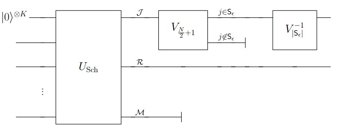
Figure 1: A quantum circuit for encoding. The Schur transform turns the initial $N$ qubits together with $K=O(\log N)$ ancillary qubits into three registers: the index register $\mathcal{J}$, the representation register $\mathcal{R}$, and the multiplicity register $\mathcal{M}$. The multiplicity register is discarded. The index register is encoded into $N/2+1$ qubits by the position embedding $V_{N/2+1}$. The qubits in positions outside $\mathsf{S}_{\epsilon}$ are discarded and the remaining qubits are reencoded into $\lceil\log|\mathsf{S}_{\epsilon}|\rceil$ qubits.

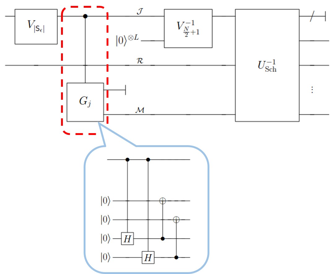
Figure 2: A quantum circuit for decoding. The first operation is the position embedding $V_{|\mathsf{S}_{\epsilon}|}$, which produces $|\mathsf{S}_{\epsilon}|$ output qubits. The $j$th of these qubits controls the generation of a maximally mixed state of rank $m_{j}$ (achieved by the controlled operation $G_{j}$, represented explicitly in the blue inset for $m_{j}=4$). The third step is the initialization of $L=N/2+1-|\mathsf{S}_{\epsilon}|$ qubits which are put in positions corresponding to values of $j$ outside $\mathsf{S}_{\epsilon}$. After a total of $N/2+1$ qubits are in place, the inverse of the position embedding is performed, followed by the inverse of the Schur transform. The output of the circuit is a state on $N$ qubits and $K=O(\log N)$ ancillas, which are finally discarded.

Let us now discuss the complexity of the compression protocol. To operate on the input state we use the Schur transform Harrow (2005); Bacon et al. (2006); Plesch and Bužek (2010), which transforms the initial $N$ qubits together with $O(\log N)$ ancillary qubits into three registers: (i) the index register, where the value of $j$ is stored into the state of $\log(N/2+1)$ qubits, (ii) the representation register, which uses $\log(N+1)$ qubits to encode the representation spaces, and (iii) the multiplicity register, where the multiplicity spaces are encoded into $O(N)$ qubits (see Fig. 1). Since the implementation of the Schur transform in a quantum circuit is approximate, we focus on approximate compression, so that the Schur transform error can be absorbed into the compression error. Let us analyze first the encoding. The first step is the approximate Schur transform, whose complexity is ${\rm poly}(N,\log 1/\epsilon^{\prime})$, $\epsilon^{\prime}$ being the approximation error Harrow (2005); Bacon et al. (2006). We set $\epsilon^{\prime}$ to be vanishing exponentially in $N$, resulting in a complexity ${\rm poly}(N)$ for the implementation of the Schur transform. After the Schur transform has been performed, the encoding circuit embeds the index register into an exponentially larger register of $N/2+1$ qubits, transforming the state $|j\rangle$ into the state where the $j$th qubit is set to $|1\rangle$ and the rest of the qubits are set to $|0\rangle$ Plesch and Bužek (2010). We refer to this transformation as position embedding and denote it by $V_{D}$, where $D$ is the dimension of the register that is being embedded (in this case $D=N/2+1$). The point of position embedding is to physically encode the value of $j$ in a form that makes it easy to check whether or not $j$ belongs to the set $S_{\epsilon}$. In fact, such a check can be equivalently implemented on a classical computer. After this step, the circuit discards the qubits in positions outside the set $S_{\epsilon}$ and transforms the remaining qubits into $\log|S_{\epsilon}|$ qubits, by applying $V^{-1}_{|S_{\epsilon}|}$. Now, the complexity of position embedding is upper bounded by $D(\log D)^{2}$ Plesch and Bužek (2010). Since $j$ ranges from 0 to $N/2$, the total complexity of the position embedding and of its inverse scales as $N(\log N)^{2}$. From the above reasoning, it is clear that the bottleneck of the encoding is the implementation of the Schur transform, which leads to an overall complexity of ${\rm poly}(N)$ for the encoding circuit. The situation is similar for the decoding, which also uses position embedding to perform operations depending on $j$ (see Fig. 2). The only new parts are the initialization of $N/2+1-|\mathsf{S}_{\epsilon}|$ qubits in the index register and the preparation of maximally mixed states of rank $m_{j}$ in the multiplicity register, which can be approximately generated with exponential precision in $O(N^{2})$ operations sup . Summing over the values of $j$ in $\mathsf{S}_{\epsilon}$, we then obtain a number of operations upper bounded by $O(N^{2})|\mathsf{S}_{\epsilon}|=O(N^{5/2})$. From the above count it is clear that the overall complexity is polynomial in $N$. In addition to the computational complexity, it is worth discussing the size of the ancillary systems needed in our compression protocol. Since the multiplicity register is discarded, the Schur transform in our protocol needs only an ancilla of $O(\log N)$ qubits Blume-Kohout et al. (2012). The position embeddings require ancillas of size $O(N)$, but, as mentioned earlier, they can be implemented on a classical computer. Hence, the total number of qubits that need to be kept coherent throughout our protocol scales only as $O(\log N)$.

Our compression protocol, presented for qubits, can be generalized to quantum systems of arbitrary dimension $d$. In this case, an ensemble of $N$ identically prepared rank-$r$ states with known spectrum can be compressed with error less than $\epsilon$ into approximately $\left(2dr-r^{2}-1\right)/2\,\log N$ qubits. In addition, one can take advantage of the presence of degeneracies and further reduce the number of qubits: every time the same eigenvalue appears in the spectrum the number of qubits is reduced by at least $1/2\log N$(see sup for the exact value). Again, the protocol can be implemented efficiently and is optimal under suitable symmetry assumptions sup .

In this Letter we showed how to efficiently store ensembles of identically prepared quantum systems into an exponentially smaller memory space. For mixed states we discovered that, whenever a nonzero error is allowed, the size of the memory is cut down in a discontinuous way, provided that the spectrum of the state is known with sufficient precision. Intriguingly, the dropoff in the memory size takes place as soon as the prior information about the eigenvalues is more than the information that could be extracted by a measurement on the input copies. Our approximate compression protocols can be implemented efficiently on a quantum computer.

Acknowledgments. We thank M. Ozols and the referees of this Letter for a number of comments that stimulated substantial improvements of the original manuscript. This work is supported by the National Natural Science Foundation of China through Grant No. 11450110096, by the Foundational Questions Institute (Grant No. FQXi-RFP3-1325), by the 1000 Youth Fellowship Program of China, and by the HKU Seed Funding for Basic Research.

Appendix A PROOF OF THEOREM 1

Here we show the optimality of our the error protocol in the main text. Specifically, we show that no zero-error protocol exists that compresses a complete ensemble of mixed states into less than $\lceil 2\log(N+2)-2\rceil$.

A.1 The zero error condition

The condition for zero-error compression requires that the average error defined as

$$e_{N}=\sum_{\mathbf{n}}\,p_{\mathbf{n}}\frac{\left\|\rho^{\otimes N}_{\mathbf{n}}-\mathcal{D}\circ\mathcal{E}\left(\rho_{\mathbf{n}}^{\otimes N}\right)\right\|}{2}=0\,\,.$$ (7)

This condition immediately implies $\|\mathcal{D}\circ\mathcal{E}(\rho_{\mathbf{n}}^{\otimes N})-\rho_{\mathbf{n}}^{\otimes N}\|=0$ for every $\mathbf{n}$ except for a zero-measure set. Since the Hermitian operator $\mathcal{D}\circ\mathcal{E}(\rho_{\mathbf{n}}^{\otimes N})-\rho_{\mathbf{n}}^{\otimes N}$ has only zero eigenvalues, it must be a null operator. Hence, the channel $\mathcal{C}:=\mathcal{D}\circ\mathcal{E}$ must fix $\rho_{\mathbf{n}}^{\otimes N}$, namely that

$$\mathcal{C}(\rho_{\mathbf{n}}^{\otimes N})=\rho_{\mathbf{n}}^{\otimes N}$$ (8)

for every $\mathbf{n}$ except for a set of zero measure. Since $p_{\mathbf{n}}$ has full support on the Bloch sphere, the above condition holds for a dense set of points on the Bloch sphere. As a result, for every Bloch vector $\mathbf{n}$ there exists a sequence $\left\{\rho_{\mathbf{n}_{k}}^{\otimes N}\right\}$ of Bloch vectors satisfying Eq. (8) such that $\lim_{k\to\infty}\mathbf{n}_{k}=\mathbf{n}$ and

$$\lim_{k\to\infty}\rho_{\mathbf{n}^{\prime}_{k}}^{\otimes N}=\rho_{\mathbf{n}}^{\otimes N}\,.$$

Consequently, we have

$$\left\|\mathcal{D}\circ\mathcal{E}(\rho_{\mathbf{n}}^{\otimes N})-\rho_{\mathbf{n}}^{\otimes N}\right\|_{1} =\left\|\mathcal{D}\circ\mathcal{E}\left(\lim_{k\to\infty}\rho_{{\mathbf{n}}^{\prime}_{k}}^{\otimes N}\right)-\lim_{k\to\infty}\rho_{{\mathbf{n}}^{\prime}_{k}}^{\otimes N}\right\|$$

$$=\left\|\lim_{k\to\infty}\left[\mathcal{D}\circ\mathcal{E}(\rho_{{\mathbf{n}}^{\prime}_{k}}^{\otimes N})-\rho_{{\mathbf{n}}^{\prime}_{k}}^{\otimes N}\right]\right\|$$

$$=0,$$

which implies that $\mathcal{C}(\rho_{\mathbf{n}}^{\otimes N})=\rho_{\mathbf{n}}^{\otimes N}$ for every vector $\mathbf{n}$ on the Bloch sphere.

A.2 The algebra associated to the fixed points of a channel

Here we develop a technique that generates fixed points of a given channel starting from an initial set of fixed points. Our technique is based on a result by Blume-Kohout et al Blume-Kohout et al. (2010) characterizes the fixed points. Specifically, Theorem 5 of Ref. Blume-Kohout et al. (2010) guarantees that one can find a decomposition of the Hilbert space as $\mathcal{H}=\bigoplus_{k}\left(\mathcal{L}_{k}\otimes\mathcal{M}_{k}\right)$, with the property that the fixed points of a given channel acting on $\mathcal{H}$ are all the operators of the form

$$A=\bigoplus_{k}\left(A^{(k)}\otimes\omega^{(k)}_{0}\right)\,,$$ (9)

where $A^{(k)}$ is an arbitrary matrix on $\mathcal{L}_{k}$ and $\omega^{(k)}_{0}$ is a fixed non-negative matrix on $\mathcal{M}_{k}$. Using this fact, we develop a technique that generates fixed points of a channel starting from an initial set of fixed points.

Proposition 1.

Let ${\rm Fix}(\mathcal{C})$ be the set of fixed points of channel $\mathcal{C}$, let $\{A_{x}\}_{x\in\mathsf{X}}\subset{\rm Fix}(\mathcal{C})$ be a subset of non-negative fixed points, and let $\mu(\operatorname{d}x)$ be a non-negative measure on $\mathsf{X}$. Then, the set of operators

$$\mathcal{A}=E^{-1/2}\,{\rm Fix}(\mathcal{C})\,E^{-1/2}\,,\qquad E:=\int\mu(\operatorname{d}x)\,\,A_{x}\,,$$

is a matrix $\ast$-algebra (i. e. a matrix algebra closed under adjoint). Moreover, one has $E^{1/2}\mathcal{A}E^{1/2}\subseteq{\mathsf{Fix}}(\mathcal{C})$.

[Notation: for a non-invertible operator $E$, we define $E^{-1}$ as the inverse on the support of $E$.]

Proof.   Writing each operator $A_{x}$ in the form (9), we obtain

$$E=\bigoplus_{k}\left(E^{(k)}\otimes\omega_{0}^{(k)}\right)\,,\qquad E^{(k)}=\int\mu(\operatorname{d}x)A_{x}^{(k)}\,.$$

Hence, for a generic fixed point $A\in{\mathsf{Fix}}(\mathcal{C})$, decomposed as in Eq. (9), we have

$$E^{-1/2}AE^{-1/2}=\bigoplus_{k}\left[\left(E^{(k)}\right)^{-1/2}A_{k}\left(E^{(k)}\right)^{-1/2}\otimes P_{k}\,,\right]$$

where $P_{k}$ is the projector on the support of $\omega_{0}^{(k)}$. Since each $A_{k}$ is a generic operator on $\mathcal{L}_{k}$, we have

$$E^{-1/2}\,{\mathsf{Fix}}(\mathcal{C})\,E^{-1/2}=\bigoplus_{k}\left[{\mathsf{B}}(\mathcal{S}_{k})\otimes P_{k}\right]\,,$$

where ${\mathsf{B}}(\mathcal{S}_{k})$ denotes the algebra of all linear operators on the subspace $\mathcal{S}_{k}=\mathsf{Supp}\left[E^{(k)}\right]$. Hence, $\mathcal{A}=E^{-1/2}\,{\mathsf{Fix}}(\mathcal{C})\,E^{-1/2}$ is an algebra and is closed under adjoint. On the other hand, we have

$$E^{1/2}\,\mathcal{A}\,E^{1/2}=\bigoplus_{k}\left[{\mathsf{B}}(\mathcal{S}_{k})\otimes M^{(k)}_{0}\right]\,,$$

meaning that every operator in $E^{1/2}\,\mathcal{A}\,E^{1/2}$ is of the form (9)—that is, it is a fixed point. ∎

A.3 The minimal algebra required by the zero error condition

Let us apply Proposition 1 to the channel $\mathcal{C}=\mathcal{D}\circ\mathcal{E}$, resulting from the concatenation of the encoding and the decoding in a generic zero-error protocol. By the zero-error condition, all the states $\rho_{\mathbf{n}}^{\otimes N}$ are fixed points. The states can be decomposed as

$$\rho_{\mathbf{n}}^{\otimes N}=\bigoplus_{j=0}^{N/2}\,q_{j,N}\,\left(\rho_{\mathbf{n},j}\otimes\frac{I_{m_{j}}}{m_{j}}\right)\,.$$ (10)

A priori, this block decomposition could be completely unrelated with the block decomposition of Eq. (9). Proving that the two decompositions coincide will be the main part of our argument.

Choosing the measure $\mu(\operatorname{d}x)$ in Proposition 1 to be the invariant measure over $\mathbf{n}$, the average operator $E$ is given by

$$E=\bigoplus_{j=0}^{N/2}\,q_{j,N}\,\left(\frac{I_{j}}{d_{j}}\otimes\frac{I_{m_{j}}}{m_{j}}\right)\,.$$

Hence, the algebra $\mathcal{A}$ defined in Proposition 1 must contain all the operators of the form

$$E^{-1/2}\,\rho_{\mathbf{n}}^{\otimes N}\,E^{-1/2}=\bigoplus_{j=0}^{N/2}\,\,\left(d_{j}\,\rho_{\mathbf{n},j}\otimes I_{m_{j}}\right)\,,$$

for every unit vector $\mathbf{n}$. Hence, $\mathcal{A}$ must contain the smallest algebra $\mathcal{A}_{\min}$ generated by the above operators. We will now characterize this algebra:

Proposition 2.

If the states in Eq. (10) are not maximally mixed, $\mathcal{A}_{\min}$ contains the matrix algebra of all operators on the symmetric subspace, corresponding to $j=N/2$ in the decomposition (10).

Proof.   Let us express the state $\rho=p|0\rangle\langle 0|+(1-p)|1\rangle\langle 1|$ as $\rho=e^{-\beta Z}/\operatorname{Tr}[e^{-\beta Z}]$, $Z=|0\rangle\langle 0|-|1\rangle\langle 1|$ for a suitable $\beta\geq 0$. By definition, for every unitary $U\in\mathsf{SU}(2)$, the algebra $\mathcal{A}_{\min}$ contains the operator

$$A_{U} :=E^{-1/2}(U\rho U^{{\dagger}})^{\otimes N}E^{-1/2}$$

$$=\bigoplus_{j=0}^{N/2}\,\frac{d_{j}}{\operatorname{Tr}\left[e^{-\beta J^{(j)}_{z}}\right]}\,\left(U^{(j)}\,e^{-\beta J^{(j)}_{z}}U^{(j){\dagger}}\otimes I_{m_{j}}\right)\,,\qquad\qquad J_{z}^{(j)}=\sum_{m=-j}^{j}\,m\,|j,m\rangle\langle j,m|$$ (11)

where $U^{(j)}$ denotes the $(2j+1)$-dimensional irreducible representation of $\mathsf{SU}(2)$. Moreover, since the algebra $\mathcal{A}_{\min}$ is closed under linear combinations, $\mathcal{A}_{\min}$ must contain the operator

$$X_{l}=\int\operatorname{d}U\,\chi_{U}^{(l)}~{}A_{U}\,,$$

where $\chi_{U}^{(l)}$ are the characters of the irreducible representations of $\mathsf{SU}(2)$ given by $\chi_{U}^{(l)}=\operatorname{Tr}[U^{(l)}]$. Let us set $l=N$. In this case, the orthogonality of $\mathsf{SU}(2)$ matrix elements eliminates all terms in the block decomposition of $\rho^{\otimes N}$, except for the term with $j=N/2$. Notice that in this case the multiplicity subspace is trivial. Hence, one has

$$X_{N} =\int\operatorname{d}U\,\chi_{U}^{(N)}\,d_{N/2}\,U^{(N/2)}\,\rho_{N/2}\,U^{(N/2){\dagger}}\qquad\qquad\rho_{N/2}=\frac{e^{-\beta J_{z}^{(N/2)}}}{\operatorname{Tr}\left[e^{-\beta J_{z}^{(N/2)}}\right]}\,.$$

The matrix elements of $X_{N}$ can be computed explicitly as

$$\left\langle\frac{N}{2},n\right|\,X_{N}\,\left|\frac{N}{2},n^{\prime}\right\rangle =\frac{d_{N/2}}{\operatorname{Tr}\left[e^{-\beta J^{(N/2)}_{z}}\right]}\,\int\operatorname{d}U\,\chi_{U}^{(N)}\,\left[\sum_{m=-N/2}^{N/2}\,e^{-\beta m}\,\left\langle\frac{N}{2},n\right|U^{(N/2)}\left|\frac{N}{2},m\right\rangle\left\langle\frac{N}{2},m\right|U^{(N/2){\dagger}}\left|\frac{N}{2},n^{\prime}\right\rangle\right]$$

$$=\delta_{n,n^{\prime}}\,(-1)^{n}\,\frac{d_{N/2}\,\left\langle\frac{N}{2},n,\frac{N}{2},-n^{\prime}|N,0\right\rangle}{d_{N}\operatorname{Tr}\left[e^{-\beta J^{(N/2)}_{z}}\right]}\,\left[\sum_{m=-N/2}^{N/2}\,(-e^{-\beta})^{m}\,\overline{\left.\left\langle\frac{N}{2},m,\frac{N}{2},-m\right|N,0\right\rangle}\right]\,$$

$$=\delta_{n,n^{\prime}}\,(-1)^{n}\,\frac{d_{N/2}\,\left\langle\frac{N}{2},n,\frac{N}{2},-n^{\prime}|N,0\right\rangle}{d_{N}\operatorname{Tr}\left[e^{-\beta J^{(N/2)}_{z}}\right]}\,\left[\sum_{m=-N/2}^{N/2}\,\,\frac{(N!)^{2}(-e^{-\beta})^{m}}{(N/2-m)!(N/2+m)!\sqrt{(2N)!}}\right]\,$$

$$=\delta_{n,n^{\prime}}\,(-1)^{n+N/2}\,\frac{d_{N/2}(N!)e^{\beta N/2}(1-e^{-\beta})^{N}\,\left\langle\frac{N}{2},n,\frac{N}{2},-n^{\prime}|N,0\right\rangle}{d_{N}\sqrt{(2N)!}\operatorname{Tr}\left[e^{-\beta J^{(N/2)}_{z}}\right]}\,,$$

$\langle j_{1},m_{1},j_{2},m_{2}|J,M\rangle$ denoting the Clebsch-Gordan coefficient. Note that the Clebsch-Gordan coefficient in the above expression is nonzero if and only if $n=n^{\prime}$. As a consequence, the operator $X_{N}$ has full support.

Now, since $\mathcal{A}_{\min}$ is an algebra, it must contain $X_{N}$ as well as the whole Abelian algebra generated by it. In particular, it must contain the projector on the support of $X_{N}$—which is nothing but $P_{N/2}$, the projector on the symmetric subspace. Moreover, it must contain all the operators of the form

$$A_{U,N/2}=P_{N/2}A_{U}P_{N/2}\propto U^{(N/2)}\,e^{-\beta J^{(N/2)}_{z}}\,U^{(N/2){\dagger}}\qquad\forall\,U\in\mathsf{SU}(2)\,.$$

Finally, for $\beta\not=0$, it is easy to see that the smallest algebra $\mathcal{A}_{\min,N/2}$ containing the above operators is the algebra $\mathsf{B}(\mathcal{R}_{N/2})$. This can be easily seen by von Neumann’s double commutant theorem: If an operator $B$ commutes with the non-degenerate Hermitian operator $A_{U,N/2}$ for every $U$, then $B$ must be proportional to the identity. Hence, the double commutant of $\mathcal{A}_{N/2}$—equal to $\mathcal{A}_{N/2}$ itself—is the whole $\mathsf{B}(\mathcal{R}_{N/2})$. In conclusion, we have the inclusion $\mathsf{B}(\mathcal{R}_{N/2})\subseteq\mathcal{A}_{\min,N/2}\subseteq\mathcal{A}_{\min}$. ∎

Proposition 3.

If the states in Eq. (10) are neither pure nor maximally mixed, then $\mathcal{A}_{\min}$ is the full algebra generated by the $N$-fold tensor representation of $\mathsf{GL}(2)$, namely

$$\mathcal{A}_{\min}=\bigoplus_{j=0}^{N/2}\,\left[\mathsf{B}(\mathcal{R}_{j})\otimes I_{m_{j}}\right]\,,$$

$\mathsf{B}(\mathcal{R}_{j})$ denoting the algebra of all linear operators on the representation space $\mathcal{R}_{j}$.

Proof.   We prove that $\mathcal{A}_{\min}$ contains the algebra $\mathsf{B}(\mathcal{R}_{j})\otimes I_{m_{j}}$ for every $j$. The proof is by induction, with $j$ starting from $N/2$ and going down to $0$. For $j=N/2$ we know that $\mathcal{A}_{\min}$ contains the algebra $\mathsf{B}(\mathcal{R}_{N/2})$ of all operators with support in the symmetric subspace. Let us assume that $\mathcal{A}_{\min}$ contains all the algebras $\mathsf{B}(\mathcal{R}_{j})\otimes I_{m_{j}}$ with $j\geq j_{*}+1$ and show that it must necessarily contain also the algebra $\mathsf{B}(\mathcal{R}_{j_{*}})\otimes I_{m_{j_{*}}}$. By construction, we know that $\mathcal{A}_{\min}$ contains all the operators $A_{U}$ of the form

$$A_{U}=\bigoplus_{j=0}^{N/2}\,\frac{d_{j}}{\operatorname{Tr}\left[e^{-\beta J^{(j)}_{z}}\right]}\,\left(U^{(j)}\,e^{-\beta J^{(j)}_{z}}U^{(j){\dagger}}\otimes I_{m_{j}}\right)\,,\qquad\qquad J_{z}^{(j)}=\sum_{m=-j}^{j}\,m\,|j,m\rangle\langle j,m|\,.$$

Since the states in Eq. (10) are not pure, all the blocks in the sum are non-zero. Moreover, the induction hypothesis implies that $\mathcal{A}_{\min}$ should also contain the operators $A_{U}^{\prime}$ of the form

$$A_{U}^{\prime}=\bigoplus_{j=0}^{j_{*}}\,\frac{d_{j}}{\operatorname{Tr}\left[e^{-\beta J^{(j)}_{z}}\right]}\,\left(U^{(j)}\,e^{-\beta J^{(j)}_{z}}U^{(j){\dagger}}\otimes I_{m_{j}}\right)\,,\qquad U\in SU(2)\,.$$

Now, we can repeat the argument used in the proof of Proposition 2: by linearity, $\mathcal{A}_{\min}$ must contain the operator

$$X_{2j_{*}} =\int\operatorname{d}U\,\chi_{U}^{(2j_{*})}~{}A^{\prime}_{U}$$

$$=\frac{d_{j_{*}}}{\operatorname{Tr}\left[e^{-\beta J^{(j_{*})}_{z}}\right]}\int\operatorname{d}U\,\chi_{U}^{(2j_{*})}~{}\,\left(U^{(j_{*})}\,e^{-\beta J^{(j_{*})}_{z}}\,U^{(j_{*}){\dagger}}\otimes I_{m_{j_{*}}}\right)\,.$$

Explicit calculation (same as in Proposition 2) shows that $X_{2j_{*}}$ has full rank. Hence, the projector on the support of $X_{2j_{*}}$ is $P_{j_{*}}=I_{j_{*}}\otimes I_{m_{j_{*}}}$. Since $\mathcal{A}_{\min}$ should contain this projector, it must also contain all operators of the form

$$A^{\prime}_{U,j_{*}} =P_{j_{*}}A^{\prime}_{U}P_{j_{*}}$$

$$\propto U^{(j_{*})}e^{-\beta J^{(j_{*})}_{z}}U^{(j_{*}){\dagger}}\otimes I_{m_{j_{*}}}\,,\qquad U\in SU(2)\,.$$

Again, using von Neumann’s double commutant theorem, it is easy to show that the smallest algebra containing all the above operators is $\mathsf{B}(\mathcal{R}_{j^{*}})\otimes I_{m_{j_{*}}}$. In conclusion we proved that $\mathcal{A}_{\min}$ must contain $\mathsf{B}(\mathcal{R}_{j^{*}})\otimes I_{m_{j_{*}}}$. By induction, this proves the inclusion

$$\mathcal{A}_{\min}\supseteq\bigoplus_{j=0}^{N/2}\,\left[\mathsf{B}(\mathcal{R}_{j})\otimes I_{m_{j}}\right]\,.$$

In the other hand, the definition of $\mathcal{A}_{\min}$ implies the opposite inclusion. Hence, one must have the equality. ∎

A.4 Zero-error compression of a complete ensemble implies zero error compression for every ensemble of permutationally invariant states

Propositions 1 and 3 imply the following

Corollary 1.

If the states (10) are neither pure nor maximally mixed, every channel $\mathcal{C}$ preserving them must preserve all permutationally invariant states.

Proof.   By Propositions 1 and 3, the channel $\mathcal{C}$ must satisfy

$${\mathsf{Fix}}(\mathcal{C})\supseteq\mathcal{A}_{\min}=\bigoplus_{j=0}^{N/2}\,\left[\mathsf{B}(\mathcal{R}_{j})\otimes I_{m_{j}}\right]\,,$$

meaning that the full algebra generated by the tensor representation of $\mathsf{GL}(2)$ is contained in the set of fixed points. ∎

We are now in position to prove Theorem 1 in the main text:

Proof of Theorem 1. Suppose that a compression protocol has zero error on a complete ensemble of mixed states. Then, Corollary 1 implies that the protocol should have zero error on all permutationally invariant states. In particular, the protocol should be able to transmit without error the following ensemble of orthogonal pure states

$$S:=\left.\left\{\rho_{j,m}=|j,m\rangle\langle j,m|\otimes\frac{I_{m_{j}}}{m_{j}},p_{j,m}=\frac{1}{D}\,\right|\,j=0,\dots,N/2\,,m=-j,\dots,j,\,D:=\sum_{j}d_{j}\right\}\,.$$

A lower bound on the dimension $d_{\rm enc}$ of the encoding space $\mathcal{H}_{\rm enc}$ is then obtained by considering the amount of classical information carried by $S$. In detail, the lower bound can be calculated using the monotonicity of Holevo’s chi quantity in quantum data processing. Holevo’s chi quantity of $S$ Holevo (1973) is defined as follows

$$\chi\left(S\right) :=H\left(\sum_{j,m}p_{j,m}\rho_{j,m}\right)-\sum_{j,m}p_{j,m}H\left(\rho_{j,m}\right)$$

with $H(\rho)$ being the von Neumann entropy of the state $\rho$. Since the chi quantity is non-increasing under quantum evolutions, in the zero-error scenario we have

$$\chi\left(S\right)=\chi\left(S_{\rm enc}\right)$$ (12)

where $S_{\rm enc}$ is the encoded ensemble $S_{\rm enc}:=\{\mathcal{E}(\rho_{j,m}),p_{j,m}\}$. On the other hand, the dimension of the encoding subspace is lower bounded by the chi quantity Horodecki (1998)

$$\log d_{\rm enc}\geq\chi\left(S_{\rm enc}\right).$$ (13)

The chi quantity for the ensemble $S$ can be computed as $\chi\left(S\right)=\log D\,.$ Combining this equality with Eqs. (12) and (13) we get

$$d_{\rm enc}\geq D=\left(\frac{N}{2}+1\right)^{2},$$

which concludes the optimality proof. The protocol showed in the main text saturates the bound. ∎

Appendix B PROOF OF THEOREM 2

As stated in the main text, we assume $p>\frac{1}{2}$, because for $p=1/2$ the ensemble is trivial, consisting only of the maximally mixed state.

We first notice that the error of the compression protocol is upper bounded as

$$e_{N} =\frac{1}{2}\,\left\|\rho_{\mathbf{n}}^{\otimes N}-\mathcal{D}\circ\mathcal{E}\left(\rho_{\mathbf{n}}^{\otimes N}\right)\right\|\,,\qquad\forall\mathbf{n}\in\mathbb{S}^{2}$$

$$=\frac{1}{2}\,\left\|\sum_{j\not\in\mathsf{S}_{\epsilon}}\,q_{j,N}\,\left[\rho_{\mathbf{n},j}\otimes\frac{I_{m_{j}}}{m_{j}}-\mathcal{D}(\rho_{0})\right]\right\|$$

$$\leq\sum_{j\not\in\mathsf{S}_{\epsilon}}q_{j,N}\,,$$ (14)

the last step following from the triangle inequality and from the fact that the trace distance of two states is upper bounded by 2. Note that the upper bound is independent of $\mathbf{n}$, meaning that the protocol works equally well for all states with the same spectrum (or equivalently, for all states with the same purity).

At this point, it is enough to prove that the upper bound vanishes in the large $N$ limit. To this purpose, we use the expression for $q_{j,N}$ [Eq. (5) in the main text] and observe that one has

$$1-e_{N}\geq \sum_{j\in\mathsf{S}_{\epsilon}}\frac{2(2j+1)}{j_{0}}B\left(N+1,p,\frac{N}{2}+j+1\right)-\sum_{j\in\mathsf{S}_{\epsilon}}\frac{2(2j+1)}{j_{0}}B\left(N+1,p,\frac{N}{2}-j\right)$$ (15)

where $j_{0}=(2p-1)(N+1)/2$. The second summand in the r.h.s. of Eq. (15) is negligible in the large $N$ limit: precisely, it can be bounded as

$$\sum_{j\in\mathsf{S}_{\epsilon}}\frac{2(2j+1)}{j_{0}}B\left(N+1,p,\frac{N}{2}-j\right) \leq \sum_{j=0}^{\frac{N}{2}}\frac{2(2j+1)}{j_{0}}B\left(N+1,p,\frac{N}{2}-j\right)$$ (16)

$$\leq \frac{1}{2p-1}\sum_{j=0}^{\frac{N}{2}}B\left(N+1,p,\frac{N}{2}-j\right)$$

$$\leq \frac{1}{2p-1}\exp\left[-\frac{2(2p-1)^{2}N^{2}}{N+1}\right]$$

having used the Hoeffding’s inequality in the last step. Hence, this term goes to zero exponentially fast with $N$,

Now, recall that we chose $\mathsf{S}_{\epsilon}$ to be the interval

$$\mathsf{S}_{\epsilon}=\left[j_{0}-1/2-\sqrt{N\ln(2/\epsilon)},j_{0}-1/2+\sqrt{N\ln(2/\epsilon)}\right].$$ (17)

Setting $j_{0}-j-1/2=x$, we then obtain

$$e_{N} \leq 1-\sum_{x=-\sqrt{N\ln(2/\epsilon)}}^{\sqrt{N\ln(2/\epsilon)}}\left(1-\frac{x}{j_{0}}\right)B\left(N+1,p,p(N+1)-x\right)+\frac{1}{2p-1}\exp\left[-\frac{2(2p-1)^{2}N^{2}}{N+1}\right]$$

$$=1-\sum_{x=-\sqrt{N\ln(2/\epsilon)}}^{\sqrt{N\ln(2/\epsilon)}}B\left(N+1,p,p(N+1)-x\right)+\frac{1}{2p-1}\exp\left[-\frac{2(2p-1)^{2}N^{2}}{N+1}\right]$$

$$\leq 2\exp\left[\frac{2N}{N+1}\ln\frac{\epsilon}{2}\right]+\frac{1}{2p-1}\exp\left[-\frac{2(2p-1)^{2}N^{2}}{N+1}\right]$$

$$\leq\epsilon^{\frac{2N}{N+1}}+\frac{1}{2p-1}\exp\left[-\frac{2(2p-1)^{2}N^{2}}{N+1}\right]$$

In the second last step we have used the Hoeffding’s inequality. Now it can be seen that the right hand side of the bound vanishes exponentially fast with $N$, and we can always find a $N_{0}$ such that $e_{N}\leq\epsilon^{3/2}<\epsilon$ for any $N>N_{0}$. The dimension of the encoded system is now

$$d_{\rm enc} = \sum_{j\in\mathsf{S}_{\epsilon}}(2j+1)$$

$$= 2(2p-1)\sqrt{N\ln(2/\epsilon)}(N+1)$$

An upper bound on the number of required qubits is given by

$$\log d_{\rm enc} =\log\left[2(2p-1)N\sqrt{N\ln\frac{2}{\epsilon}}\right]+\log\left(1+\frac{1}{N}\right)$$

$$\leq\frac{3}{2}\log N+\log\left[2(2p-1)\sqrt{\ln\frac{2}{\epsilon}}\right]+1$$

∎

Appendix C THE PURE STATE CASE: NO DISCONTINUOUS GAP BETWEEN ZERO-ERROR AND APPROXIMATE COMPRESSION

Here we prove that the type of discontinuity highlighted by our Theorems 1 and 2 is specific to mixed states. Consider the pure state ensemble $\left\{\left(|\mathbf{n}\rangle\langle\mathbf{n}|\right)^{\otimes N}\,,\operatorname{d}^{2}\mathbf{n}\right\}$, where $|\mathbf{n}\rangle$ is the pure qubit state with Bloch vector $\mathbf{n}$ and $\operatorname{d}^{2}\mathbf{n}$ is the invariant measure on the Bloch sphere. Suppose that the state $\left(|\mathbf{n}\rangle\langle\mathbf{n}|\right)^{\otimes N}$ is encoded into a state $\rho_{\mathbf{n},{\rm enc}}$ on a Hilbert space of dimension $d_{\rm enc}$. Assuming that the compression error is bounded by $\epsilon$, an argument by Horodecki Horodecki (1998) gives a lower bound on $d_{\rm enc}$. The argument is based on the following lemma, based on the Alicki-Fannes inequality

Lemma 1 (Alicki and Fannes (2004)).

Let $\{\rho_{x}\,,p_{x}\}$ be an ensemble of states and let $\{\rho_{x,{\rm enc}}\,,p_{x}\}$ be the ensemble of the encoded states. If the compression protocol has error bounded by $\epsilon$, then the following inequality holds

$$\left|\chi\left(\left\{\rho_{x}\,,p_{x}\right\}\right)-\chi\left(\left\{\rho_{x,{\rm enc}}\,,p_{x}\right\}\right)\right|\leq 2\left[\epsilon\log d_{\rm in}+\eta(\epsilon)\right],$$ (18)

where $d_{\rm in}$ is the rank of the average state $\rho=\sum_{x}\,p_{x}\rho_{x}$ and $\eta(x)=-x\ln x$.

In our case, $d_{\rm in}$ is the dimension of the symmetric subspace, namely

$$d_{\rm in}=d_{\frac{N}{2}}=N+1\,.$$ (19)

Moreover, we have

$$\chi\left(\left\{\left(|\mathbf{n}\rangle\langle\mathbf{n}|\right)^{\otimes N},\,\operatorname{d}^{2}\mathbf{n}\right\}\right)=H\left(I_{\frac{N}{2}}/d_{\frac{N}{2}}\right)=\log(N+1).$$ (20)

and, by the Holevo’s bound Holevo (1973),

$$\chi\left(\left\{\rho_{\mathbf{n},{\rm enc}}\,,\operatorname{d}^{2}\mathbf{n}\right\}\right)\leq\log d_{\rm enc}\,.$$ (21)

In our case, we have $d_{\rm in}=d_{\frac{N}{2}}=N+1$. Hence, combining Eqs. (18), (19), (20), and (21) we obtain the bound

$$\log d_{\rm enc} \geq(1-2\epsilon)\log(N+1)-2\eta(\epsilon).$$

Now, note that the r.h.s. is continuous in $\epsilon$ and tends to $\log(N+1)$ when $\epsilon$ tends to zero. The value $\log(N+1)$ is exactly the minimum number of qubits needed to encode a generic state in the symmetric subspace with zero error. Hence, as $\epsilon$ tends to zero, the number of qubits needed for approximate compression tends to the number of qubits needed for zero-error compression.

Appendix D PROOF OF THEOREM 3

Here we prove the optimality of our protocol among all compression protocols where the encoding is covariant and the decoding preserves the magnitude of the total angular momentum. Precisely, we assume that

1. the encoding space $\mathcal{H}_{\rm enc}$ supports a unitary representation of the group $\mathsf{SU}(2)$, denoted by $\{V_{g}~{}|~{}g\in\mathsf{SU}(2)\}$

2. the encoding channel satisfies the covariance condition

   $$\mathcal{E}\circ\mathcal{U}_{g}=\mathcal{V}_{g}\circ\mathcal{E}\,,\qquad\forall g\in\mathsf{SU}(2)\,,$$ (22)

   where $\mathcal{U}_{g}$ and $\mathcal{V}_{g}$ are the unitary channels defined by $\mathcal{U}_{g}(\cdot):=U_{g}\cdot U_{g}^{\dagger}$ and $\mathcal{V}_{g}=V_{g}\cdot V_{g}^{\dagger}$.

3. the decoding channel $\mathcal{D}$ preserve the magnitude of the total angular momentum, in the sense that, for every input state $\rho$, one has

   $$\operatorname{Tr}\left[\mathbf{K}^{2}\,\mathcal{D}(\rho)\right]=\operatorname{Tr}\left[\mathbf{J}^{2}\,\rho\right]\,,$$ (23)

   where $\mathbf{K}=(K_{x},K_{y},K_{z})$ are the generators of the representation $\{V_{g}\,,g\in\mathsf{SU}(2)\}$ and $\mathbf{J}=(J_{x},J_{y},J_{z})$ are the generators of the representation $\{U_{g}^{\otimes N},g\in\mathsf{SU}(2)\}$.

Under these conditions, we can prove the optimality of the protocol presented in Theorem 3 of the main text.

Proof of Theorem 3. For the purpose of this proof, it is convenient to parametrize the mixed states $\rho_{\mathbf{n}}$ as $\rho_{g}=U_{g}\rho U_{g}^{\dagger}$, where $\rho$ is a fixed state and $g$ is a generic element of $\mathsf{SU}(2)$. Let us decompose the encoding space as

$$\mathcal{H}_{\rm enc}=\bigoplus_{j}\,\left(\mathcal{R}_{j}\otimes\widetilde{\mathcal{M}}_{j}\right)\,,$$ (24)

where $j$ is the quantum number of the angular momentum, $\mathcal{R}_{j}$ is the corresponding representation space, and $\widetilde{\mathcal{M}}_{j}$ is a suitable multiplicity space. By definition, one has

$$\mathcal{H}_{\rm enc} \supseteq\mathsf{Span}\left\{\mathsf{Supp}\left[\mathcal{E}\left(\rho_{g}^{\otimes N}\right)\right],g\in\mathsf{SU}(2)\right\}$$

$$=\mathsf{Span}\left[\mathsf{Supp}\left(\Omega\right)\right]\,,\qquad\Omega:=\int\operatorname{d}g\,\mathcal{E}\left(\rho_{g}^{\otimes N}\right)\,.$$ (25)

Since $\mathcal{E}$ is covariant, the state $\Omega$ satisfies the relation $V_{g}\Omega V_{g}^{\dagger}=\Omega\,,\forall g\in\mathsf{SU}(2)$. Hence, $\Omega$ can be written in the block diagonal form

$$\Omega=\bigoplus_{j\in\mathsf{S}}\left(\frac{I_{j}}{d_{j}}\otimes\omega_{j}\right)\,,$$

where $\omega_{j}$ is a suitable state on the multiplicity space and $\mathsf{S}$ is a suitable set of values of the angular momentum number. Combining the above decomposition with Eq. (25), we obtain the bound

$$d_{\rm enc}\geq\mathsf{rank}\,\Omega\geq\sum_{j\in\mathsf{S}}\,d_{j}\,.$$ (26)

On the other hand, since the decoding preserves the magnitude of the angular momentum, one has

$$\operatorname{Tr}[\Pi_{j}\,\mathcal{D}\circ\mathcal{E}\left(\rho_{g}^{\otimes N}\right)] =\operatorname{Tr}[\widetilde{\Pi}_{j}\mathcal{E}\left(\rho_{g}^{\otimes N}\right)]\,,\qquad\forall j=0,\dots,N/2\,,\forall g\in\mathsf{SU}(2)\,,$$

where $\Pi_{j}$ is the projector on $\mathcal{R}_{j}\otimes\mathcal{M}_{j}$ while $\widetilde{\Pi}_{j}$ is the projector on $\mathcal{R}_{j}\otimes\widetilde{\mathcal{M}}_{j}$. Hence, we have

$$\sum_{j\in\mathsf{S}}\operatorname{Tr}[\Pi_{j}\mathcal{D}\circ\mathcal{E}\left(\rho_{g}^{\otimes N}\right)]=1\,,\qquad\forall g\in\mathsf{SU}(2)\,,$$ (27)

meaning that all the output states $\mathcal{D}\circ\mathcal{E}\left(\rho_{g}^{\otimes N}\right)$ are contained in the subspace $\mathcal{H}_{N}:=\bigoplus_{j\in\mathsf{S}}\left(\mathcal{R}_{j}\otimes\mathcal{M}_{j}\right)$. Hence, we have

$$e_{N} =\frac{1}{2}\left\|\rho_{g}^{\otimes N}-\ \mathcal{D}\circ\mathcal{E}\left(\rho_{g}^{\otimes N}\right)\right\|\qquad\forall g\in\mathsf{SU}(2)$$

$$\geq\frac{1}{2}\left\|P_{N}\left[\rho_{g}^{\otimes N}-\ \mathcal{D}\circ\mathcal{E}\left(\rho_{g}^{\otimes N}\right)P_{N}\right]\right\|+\frac{1}{2}\left\|(I^{\otimes N}-P_{N})\left[\rho_{g}^{\otimes N}-\ \mathcal{D}\circ\mathcal{E}\left(\rho_{g}^{\otimes N}\right)\right](I^{\otimes N}-P_{N})\right\|$$

$$=\frac{1}{2}\left\|(I^{\otimes N}-P_{N})\rho_{g}^{\otimes N}(I^{\otimes N}-P_{N})\right\|$$

$$\geq\sum_{j\not\in\mathsf{S}}\frac{q_{j,N}}{2}$$ (28)

where $P_{N}$ is the projector on $\mathcal{H}_{N}$. Now we prove that any protocol with $d_{\rm enc}=O\left(N^{3/2-\delta}\right)$, $\delta>0$, will have a non-vanishing error. Recall from the main text that the probability distribution $q_{j,N}$ can be expressed as

$$q_{j,N}=\frac{2j+1}{2j_{0}} \left[B\left(N+1,p,\frac{N}{2}+j+1\right)-B\left(N+1,p,\frac{N}{2}-j\right)\right]$$ (29)

where $B(n,p,k)$ is the binomial distribution with $n$ trials and with probability $p$ and

$$j_{0}=(p-1/2)(N+1)\,.$$

Combing Eq. (28) with Eq. (29), we have

$$e_{N} \geq\frac{1}{2}-\frac{1}{2}\sum_{j\in\mathsf{S}}\frac{2j+1}{2j_{0}}B\left(N+1,p,\frac{N}{2}+j+1\right).$$

We split the set $\mathsf{S}$ into two subsets $\mathsf{S}_{1}$ and $\mathsf{S}_{2}$, defined as

$$\mathsf{S}_{1} =\mathsf{S}\cap\left[j_{0}-\frac{\sqrt{cN}+1}{2},j_{0}+\frac{\sqrt{cN}+1}{2}\right]$$

$$\mathsf{S}_{2} =\mathsf{S}\setminus\mathsf{S}_{1}$$

where $c$ is an arbitrary constant. The error is then bounded as

$$e_{N} \geq\frac{1}{2}\left(1-s_{1}-s_{2}\right)\,\qquad s_{k}:=\sum_{j\in\mathsf{S}_{k}}\frac{2j+1}{2j_{0}}B\left(N+1,p,\frac{N}{2}+j+1\right)\,,~{}k=1,2\,.$$ (30)

We now bound $s_{1}$ and $s_{2}$. Let us start from $s_{1}$: by definition, we have

$$s_{1} \leq\frac{\max_{j\in\mathsf{S}_{1}}(2j+1)}{2j_{0}}\,\sum_{j\in\mathsf{S}_{1}}B\left(N+1,p,\frac{N}{2}+j+1\right)$$

$$=O(1)\,\sum_{j\in\mathsf{S}_{1}}B\left(N+1,p,\frac{N}{2}+j+1\right)$$

$$\leq O(1)\,|\mathsf{S}_{1}|B\left(N+1,p,\frac{N}{2}+j_{0}+1\right)$$

$$=O\left(N^{-1/2}\right)\,|\mathsf{S}_{1}|\,.$$ (31)

In turn, $\mathsf{S}_{1}$ can be bounded from the relation

$$|\mathsf{S}_{1}|\,\left(\min_{j\in\mathsf{S}_{1}}\,2j+1\right) \leq\sum_{j\in\mathsf{S}_{1}}(2j+1)$$

$$\leq d_{\rm enc}$$

$$=O\left(N^{3/2-\delta}\right)\,,$$ (32)

which implies $|\mathsf{S}_{1}|\leq O(N^{1/2-\delta})$. Inserting this relation into Eq. (31), we finally obtain

$$s_{1}\leq O\left(N^{-\delta}\right)\,.$$ (33)

Regarding $s_{2}$, we have the bound

$$s_{2} \leq\frac{N+1}{j_{0}}\left[\sum_{j\leq j_{0}-\frac{\sqrt{cN}+1}{2}}\,B\left(N+1,p,\frac{N}{2}+j+1\right)\right]$$

$$=\frac{1}{p-1/2}\left[\sum_{j\leq j_{0}-\frac{\sqrt{cN}+1}{2}}\,B\left(N+1,p,\frac{N}{2}+j+1\right)\right]$$

$$\leq\frac{e^{-c/2}}{p-1/2}\,,$$ (34)

the last inequality coming from Hoeffding’s bound.

Finally, combining the inequalities (30), (33), and (34), we obtain the lower bound

$$e_{N}\geq\frac{1}{2}\left[1-O\left(N^{-\delta}\right)-\frac{e^{-c/2}}{p-1/2}\right]\,,$$

Since the constant $c$ is arbitrary, the bound becomes $e_{N}\geq 1/2-O\left(N^{-\delta}\right)$. ∎

Appendix E UPPER BOUND ON THE COMPLEXITY OF GENERATING APPROXIMATE MAXIMALLY MIXED STATES

The decoding requires the preparation of maximally mixed states to be placed in the multiplicity register. For a given value of $j$, this is accomplished by generating a maximally entangled state of rank $m_{j}$. In the following we present a three-step protocol for this purpose.

1. Choose an integer $n=O(N)$ such that $m_{j}\in(2^{n-1},2^{n}]$. Prepare $n$ maximally entangled qubit states. The resulting the state is $\rho=[|\Phi^{+}\rangle\langle\Phi^{+}|]^{\otimes n}$, with $|\Phi^{+}\rangle=(|00\rangle+|11\rangle)/\sqrt{2}$ and lies in a space of dimension $2^{2n}$.

2. Perform the measurement in the computational basis on one qubit of each entangled pair. The measurement outcomes of the individual qubit measurements are saved in a sequence of $n$ binary digits, let us denote it by $\underline{y}$.

3. Compare the string $\underline{y}$ with the binary expression of $m_{j}$. If $\underline{y}$, as a number, is larger than $m_{j}$, the protocol fails and we have to restart by preparing again $n$ maximally entangled qubits. Otherwise, we keep the remaining qubits, which, on average, will be in a maximally entangled mixed state of rank $m_{j}$.

The last step can be seen by noting down the quantum operation $\mathcal{C}_{\rm yes}$ corresponding to the successful outcomes of the projective measurement, given by

$$\mathcal{C}_{\rm yes}(\sigma)=\sum_{y\leq m_{j}}|\underline{y}\rangle\langle\underline{y}|\sigma|\underline{y}\rangle\langle\underline{y}|\ .$$

The protocol is successful in more than half of the cases. For that reason, the probability of failure vanishes exponentially in the number of repetitions $l$ as $p_{\rm no}\leq 2^{-l}$. To ensure that the error is vanishing fast enough with the number of state copies $N$, we repeat the protocol $N$ times. Then, the complexity of the protocol is comprised of preparing the qubit states, which takes $O(N)$ steps, and from comparing the $n$ digit binary strings on a classical computer, which also takes $O(N)$ steps. By repeating the protocol $N$ times, the overall complexity yields $O(N^{2})$. It is safe to run the protocol $N$ times to assure for an exponentially vanishing error, because the complexity of the decoding is still dominated by the Schur transform.

Appendix F ZERO-ERROR COMPRESSION FOR QUANTUM SYSTEMS OF DIMENSION $d>2$

In this and the following sections, we generalize our results to quantum systems of arbitrary finite dimension $d<\infty$.

F.1 Upper bound on the number of encoding qubits

Theorem 4.

In dimension $d$, every ensemble of $N$ identically prepared mixed states of rank $r$ can be encoded without error into less than $\left(2dr-r^{2}+r-2\right)/2\,\log(N+d-1)$ qubits.

The proof is based on the Schur-Weyl duality, which allows one to decompose the $N$-copy Hilbert space as

$$\mathcal{H}^{\otimes N}\simeq\bigoplus_{\lambda\in\mathcal{Y}_{N,d}}\,\left(\mathcal{R}_{\lambda}\otimes\mathcal{M}_{\lambda}\right)\,,$$

where $\mathcal{R}_{\lambda}$ is a representation space, $\mathcal{M}_{\lambda}$ is a multiplicity space, and the sum runs over the set $\mathcal{Y}_{N,d}$ of all Young diagrams of $N$ boxes arranged in $d$ rows, parametrized as $\lambda=(\lambda_{1},\dots,\lambda_{d})$, with $\lambda_{1}\geq\lambda_{2}\geq\dots\geq\lambda_{d}$, $\sum_{i=1}^{d}\lambda_{i}=N$. We use the notations

$$d_{\lambda}=\dim\mathcal{R}_{\lambda}$$

and

$$m_{\lambda}=\dim\mathcal{M}_{\lambda}.$$

Relative to this decomposition, every state of the form $\rho^{\otimes N}$ where $\rho$ has rank $r$ can be cast into the form

$$\rho^{\otimes N}=\bigoplus_{\lambda\in\mathcal{{Y}}_{N,r}}q_{\lambda,N}\left(\rho_{\lambda}\otimes\frac{I_{m_{\lambda}}}{m_{\lambda}}\right)\,,$$

where $\rho_{\lambda}$ is a quantum state on $\mathcal{R}_{\lambda}$, $I_{m_{\lambda}}$ is the identity on $\mathcal{M}_{\lambda}$, and $q_{\lambda,N}$ is a suitable probability distribution. Note that only the Young diagrams with $r$ rows or less are present here (for this fact, see e.g. Alicki et al. (1988)).

The proof of Theorem 4 makes use of the following lemmas:

Lemma 2.

For every $\lambda\in\mathcal{{Y}}_{N,r}$, one has $d_{\lambda}\leq(N+d-1)^{(2dr-r^{2}-r)/2}$.

Proof. The dimension can be expressed as

$$d_{\lambda}=\frac{\prod_{1\leq i<j\leq d}(\lambda_{i}-\lambda_{j}-i+j)}{\prod_{k=1}^{d-1}k!}\,,$$ (35)

cf. Eq. (III.10) of Itzykson and Nauenberg (1966). Since $\lambda_{i}=0$ for $i>r$, we have the following chain of (in)equalities

$$d_{\lambda} =\frac{\prod_{1\leq i<j\leq r}(\lambda_{i}-\lambda_{j}-i+j)\,\cdot\,\prod_{1\leq i\leq r<j\leq d}(\lambda_{i}-i+j)\,\cdot\,\prod_{r<i<j\leq d}(j-i)}{\prod_{k=1}^{d-1}k!}$$

$$\leq\frac{(N+r-1)^{r\choose 2}\,\cdot\,(N+d-1)^{r(d-r)}\,\cdot\,\prod_{l=1}^{d-r-1}l!}{\prod_{k=1}^{d}k!}$$

$$\leq\frac{(N+d-1)^{(2dr-r^{2}-r)/2}}{\prod_{k=d-r}^{d-1}k!}\,.$$

∎

Lemma 3.

The total dimension of all the representation spaces corresponding to Young diagrams with no more than $r$ rows is upper bounded as

$$\sum_{\lambda\in\mathcal{{Y}}_{N,r}}\,d_{\lambda}<(N+d-1)^{\frac{2dr-r^{2}+r-2}{2}}\,.$$

Proof. By Lemma 2 one has

$$\sum_{\lambda\in\mathcal{{Y}}_{N,r}}\,d_{\lambda} \leq(N+d-1)^{\frac{2dr-r^{2}-r}{2}}\,\left|\mathcal{{Y}}_{N,r}\right|$$

$$<(N+d-1)^{\frac{2dr-r^{2}+r-2}{2}}\,,$$

having used the equality $\left|\mathcal{{Y}}_{N,r}\right|={N+r-1\choose r-1}$ Goodman and Wallach (1998) and the elementary bound ${N+r-1\choose r-1}<(N+1)^{r-1}\leq(N+d-1)^{r-1}$. ∎

Proof of Theorem 4. A zero-error compression protocol is given by the following encoding and decoding channels:

$$\mathcal{E}(\rho) =\bigoplus_{\lambda\in{\mathcal{Y}}_{N,r}}\operatorname{Tr}_{\mathcal{M}_{\lambda}}[\Pi_{\lambda}\rho\Pi_{\lambda}]$$

$$\mathcal{D}(\rho^{\prime}) =\bigoplus_{\lambda\in{\mathcal{Y}}_{N,r}}P_{\lambda}\rho^{\prime}P_{\lambda}\otimes\frac{I_{m_{\lambda}}}{m_{\lambda}}\,,$$

where $\Pi_{\lambda}$ is the projector on $\mathcal{R}_{\lambda}\otimes\mathcal{M}_{\lambda}$ and $P_{\lambda}$ is the projector on $\mathcal{R}_{\lambda}$. The encoding space is $\mathcal{H}_{\rm enc}=\bigoplus_{\lambda\in{\mathcal{Y}}_{N,r}}\mathcal{R}_{\lambda}$ and has dimension $d_{\rm enc}=\sum_{\lambda\in{\mathcal{Y}}_{N,r}}d_{\lambda}$, which we bound as

$$d_{\rm enc} =\sum_{\lambda\in{\mathcal{Y}}_{N,r}}d_{\lambda}$$

$$<(N+d-1)^{\frac{2dr-r^{2}+r-2}{2}}\,,$$

having used Lemma 3. ∎

F.2 Lower bound on the number of encoding qubits used by the zero-error protocol

Here we give a lower bound on the dimension of the encoding space in the zero-error protocol described in the proof of Theorem 4. Precisely, we have the following

Lemma 4.

The total dimension of all the representation spaces corresponding to Young diagrams with no more than $r$ rows is lower bounded as

$$\sum_{\lambda\in\mathcal{{Y}}_{N,r}}\,d_{\lambda}\geq c(r,d)\,N^{\frac{2dr-r^{2}+r-2}{2}}\,,$$ (36)

where $c$ is a suitable function.

Proof. For simplicity, we use the notation $f(N,r,d)\gtrsim g(N,r,d)$ to mean that there exists a function $c(r,d)$ such that $f(N,r,d)\geq c(r,d)g(N,r,d)$ for every $N$. If $f(N,r,d)\gtrsim g(N,r,d)$ and $g(N,r,d)\gtrsim f(N,r,d)$, then we write $f(N,r,d)\approx g(N,r,d)$. With this notation, we have

$$d_{\lambda}\gtrsim\prod_{1\leq i<j\leq d}\,(\lambda_{i}-\lambda_{j})\,,$$

having used Eq. (35). Consider the case when $N$ is a multiple of $r(r+1)/2$ and define $s=2N/r(r+1)$. Define the subset of Yang diagrams

$$\mathsf{S}_{\rm core}=\left\{\lambda\in\mathcal{Y}_{N,r}~{}|~{}\lambda_{i}\in\left[(r-i+1)s-\frac{s}{2r},(r-i+1)s+\frac{s}{2r}\right]\,,\qquad\forall i=1,\dots,r-1\right\}$$

For every diagram in $\mathsf{S}_{\rm core}$ we have the lower bound

$$d_{\lambda} \gtrsim\left[\prod_{1\leq i<j\leq r-1}\,(\lambda_{i}-\lambda_{j})\right]\,\left[\prod_{1\leq i\leq r-1}\,(\lambda_{i}-\lambda_{r})\right]\,\left[\prod_{1\leq i<r<j\leq d}\,\lambda_{i}\right]\,\left[\prod_{r<j\leq d}\,\lambda_{r}\right]$$

$$\geq\left\{\prod_{1\leq i<j\leq r}\,\left[(j-i)s-\frac{s}{r}\right]\right\}\,\left\{\prod_{1\leq i\leq r-1}\,\left[(r-i)s-\frac{s}{2}\right]\right\}\,\left\{\prod_{1\leq i\leq r<j\leq d}\,(r-i)s\right\}\,\left\{\prod_{r<j\leq d}\,\frac{s}{2}\right\}$$

$$\approx s^{\frac{2dr-r^{2}-r}{2}}$$

$$\approx N^{\frac{2dr-r^{2}-r}{2}}\,.$$ (37)

Now, the total dimension of the subspaces with Young diagrams in $\mathsf{S}_{\rm core}$ an be lower bounded as

$$\sum_{\lambda\in\mathsf{S}_{\rm core}}d_{\lambda} \gtrsim N^{\frac{2dr-r^{2}-r}{2}}\,|\mathsf{S}_{\rm core}|$$

$$=N^{\frac{2dr-r^{2}-r}{2}}\,\left(\frac{s}{r}\right)^{r-1}$$

$$\approx N^{\frac{2dr-r^{2}-r}{2}}\,N^{r-1}$$

$$=N^{\frac{2rd-r^{2}+r-2}{2}}\,.$$

Since $\mathsf{S}_{\rm core}$ is a subset of $\mathcal{Y}_{N,r}$, we obtain Eq. (36). ∎

Following the steps adopted in the $d=2$ case, it is also possible to show that the upper bound of Lemma 4 is actually an upper bound for every zero-error protocol that works for a complete ensemble of mixed states—i. e. for an ensemble of the form $\{\rho_{g}^{\otimes N}\,,p_{g}\}$ where the state $\rho_{g}$ is non-degenerate and the probability distribution $p_{g}$ is dense on $\mathsf{SU}(d)$. Essentially, the argument is based on the use of Proposition 3, which can be applied here to all the $\mathsf{SU}(2)$ subgroups of $\mathsf{SU}(d)$.

Appendix G APPROXIMATE COMPRESSION FOR QUANTUM SYSTEMS OF DIMENSION $d>2$

G.1 Compression protocol

Here we consider ensembles of $N$ identically prepared mixed states, each of them having the same spectrum. Every such ensemble can be written in the form $\{\rho_{g}^{\otimes N},p_{g}\}$, where $\rho_{g}$ is a density matrix of the form

$$\rho_{g}=U_{g}\rho_{0}U_{g}^{\dagger}\,,\qquad g\in\mathsf{SU}(d)\,,$$

$\rho_{0}$ is a rank-$r$ density matrix with non-degenerate positive eigenvalues, and $p_{g}$ is a probability distribution over the group $\mathsf{SU}(d)$. For ensembles of this form, we have the following

Theorem 5.

For every $\epsilon>0$ there exists an integer $N_{0}$ such that for every $N\geq N_{0}$ the ensemble $\{\rho_{g}^{\otimes N}\,,p_{g}\}$ can be compressed with error less than $\epsilon$ into $N_{\rm enc}$ qubits, with

$$N_{\rm enc}\leq\frac{2dr-r^{2}-1-m}{2}\log(N+d-1)+\frac{m+r-1}{2}\log\left[4d(d+1)\ln(N+1)+8\ln\left(\frac{1}{\epsilon}\right)+O\left(\frac{1}{\sqrt{N}}\right)\right]$$

and $m:=\sum_{i=1}^{r}\mu_{i}$, where $\mu_{i}$ be the cardinality of the set $\{j:\,j>i\,,p_{j}=p_{i}\}$. We notice that $m=0$ when the spectrum is non-degenerate.

The proof of the theorem is based on the Schur-Weyl decomposition

$$\rho_{g}^{\otimes N}=\bigoplus_{\lambda\in\mathcal{{Y}}_{N,r}}q_{\lambda,N}\left(U_{g}^{(\lambda)}\,\rho_{0,\lambda}\,U_{g}^{(\lambda)\,{\dagger}}\otimes\frac{I_{m_{\lambda}}}{m_{\lambda}}\right)\,,$$ (38)

where $\rho_{0,\lambda}$ is a fixed density matrix on $\mathcal{R}_{\lambda}$ and $U_{g}^{(\lambda)}$ is the irreducible representation of $\mathsf{SU}(d)$ acting on $\mathcal{R}_{\lambda}$. The key point is that the probability distribution $q_{\lambda,N}$ is concentrated on the Young diagrams such that the vector

$$p_{\lambda}:=\left(\frac{\lambda_{1}}{N},\dots,\frac{\lambda_{d}}{N}\right)$$ (39)

is close to the vector of the eigenvalues of $\rho_{0}$ O’Donnell and Wright (2015); Christandl and Mitchison (2006), listed as

$$p=(p_{1},\dots,p_{d})\,,\qquad p_{1}\geq p_{2}\geq\cdots\geq p_{r}>p_{r+1}=\cdots=p_{d}=0\,.$$ (40)

Precisely, we will use the following

Lemma 5 (O’Donnell and Wright (2015); Christandl and Mitchison (2006)).

Let $p_{\lambda}$ and $p$ be the vectors defined in Eqs. (39) and (40), respectively, and let $d(a,b):=\frac{1}{2}\sum_{i}|a_{i}-b_{i}|$ be the total variation distance between two vectors. Then, one has

$${\sf Prob}\left[\lambda:d(p_{\lambda},p)>x\right]\leq(N+1)^{d(d+1)/2}\cdot e^{-2Nx^{2}}\,,$$

with ${\sf Prob}\left[\lambda:d(p_{\lambda},p)>x\right]:=\sum_{\lambda:\,d(p_{\lambda},p)>x}\,q_{\lambda,N}$, $q_{N,\lambda}$ being the probability distribution in Eq. (38).

The idea of the proof is to discard all Young diagrams whose probability vector $p_{\lambda}$ falls outside in a ball of size $O(1/\sqrt{N})$ around the vector $p$. The dimensions of the subspaces associated to the remaining diagrams can be bounded with the following

Lemma 6.

The maximum dimension of a subspace $\mathcal{R}_{\lambda}$ satisfying $d(p_{\lambda},p)\leq x$ is upper bounded as

$$d_{\lambda}\leq(4Nx+r)^{m}\,(N+d-1)^{\frac{2dr-r(r+1)}{2}-m}\,.$$ (41)

Proof. The dimension can be bounded as

$$d_{\lambda} =\frac{\prod_{1\leq i<j\leq d}(\lambda_{i}-\lambda_{j}-i+j)}{\prod_{k=1}^{d-1}k!}$$

$$\leq\frac{\prod_{1\leq i\leq r}\left\{\left[\prod_{i<j\leq i+\mu_{i}}(\lambda_{i}-\lambda_{j}-i+j)\right]\,\left[\prod_{i+\mu_{i}<j\leq d}\,(\lambda_{i}-\lambda_{j}-i+j)\right]\right\}}{\prod_{k=1}^{d-1}k!}$$

$$\leq\frac{\prod_{1\leq i\leq r}\left\{\left[\prod_{i<j\leq i+\mu_{i}}(4Nx+\mu_{i})\right]\,\left[\prod_{i+\mu_{i}<j\leq d}\,(N+d-1)\right]\right\}}{\prod_{k=1}^{d-1}k!}$$

$$\leq\frac{\prod_{1\leq i\leq r}(4Nx+\mu_{i})^{\mu_{i}}\,(N+d-1)^{d-i-\mu_{i}}}{\prod_{k=1}^{d-1}k!}$$

$$\leq\frac{(4Nx+r)^{m}\,(N+d-1)^{\frac{2dr-r(r+1)}{2}-m}}{\prod_{k=1}^{d-1}k!}\,,$$

having used the fact that the ball $\mathsf{S}=\left\{\lambda\in\mathcal{Y}_{N,r}:\,d(p_{\lambda},p)\leq x\right\}$ is contained in the hypercube $\mathsf{S}^{\prime}=\{\lambda\in\mathcal{Y}_{N,r}:|\lambda_{i}/N-p_{i}|\leq 2x\,,\forall i=1,\dots,r-1\}$, so that, for $p_{i}=p_{j}$, $i<j$, one has $\lambda_{i}-\lambda_{j}\leq 4Nx$. ∎

Lemma 7.

The total dimension of the subspaces satisfying $d(p_{\lambda},p)\leq x$ satisfies

$$\sum_{{\lambda\in\mathcal{Y}_{N,r}:\,d(p_{\lambda},p)\leq x}}\,d_{\lambda}\leq\,(N+d-1)^{\frac{2dr-r(r+1)}{2}-m}(4Nx+r)^{m+r-1}\,.$$

Proof. Immediate from Lemma 6 and from the fact that the ball $\mathsf{S}=\left\{\lambda\in\mathcal{Y}_{N,r}:\,d(p_{\lambda},p)\leq x\right\}$ is contained in the hypercube $\mathsf{S}^{\prime}=\{\lambda\in\mathcal{Y}_{N,r}:|\lambda_{i}/N-p_{i}|\leq 2x\,,\forall i=1,\dots,r-1\}$, yielding the bound

$$|\mathsf{S}|\leq|\mathsf{S}^{\prime}|\leq(4Nx)^{r-1}\,.$$

∎

Proof of Theorem 5. To compress within an error $\epsilon$, we choose the encoding and decoding channels

$$\mathcal{E}(\rho) =\bigoplus_{\lambda\in\mathsf{S}_{\epsilon}}\operatorname{Tr}_{\mathcal{M}_{\lambda}}[\Pi_{\lambda}\rho\Pi_{\lambda}]\,\oplus\,\operatorname{Tr}\left[\rho\left(I^{\otimes N}-\Pi_{\epsilon}\right)\right]\,\rho_{\rm fail}$$

$$\mathcal{D}(\rho^{\prime}) =\bigoplus_{\lambda\in\mathsf{S}_{\epsilon}}\,\left(P_{\lambda}\rho^{\prime}P_{\lambda}\otimes\frac{I_{m_{\lambda}}}{m_{\lambda}}\right)\,,$$

with $\Pi_{\epsilon}=\bigoplus_{\lambda\in\mathsf{S}_{\epsilon}}\Pi_{\lambda}$, $\mathsf{Supp}(\rho_{\rm fail})\subseteq\mathcal{H}_{\rm enc}=\bigoplus_{\lambda\in\mathsf{S}_{\epsilon}}\,\mathcal{R}_{\lambda}$, and

$$\mathsf{S}_{\epsilon}:=\left\{\lambda\in\mathcal{{Y}}_{N,r}~{}|~{}d(p_{\lambda},p)\leq x_{\epsilon}\right\}\,,\qquad x_{\epsilon}=\sqrt{\frac{d(d+1)/2\ln(N+1)+\ln(1/\epsilon)}{2N}}\,.$$

The value of $x_{\epsilon}$ is chosen in order to bound the compression error as

$$e_{N} =\frac{1}{2}\left\|\mathcal{D}\circ\mathcal{E}\left(\rho_{g}^{\otimes N}\right)-\rho_{g}^{\otimes N}\right\|\qquad\forall g\in\mathsf{SU}(d)$$

$$\leq\frac{1}{2}\operatorname{Tr}\left[\rho\left(I^{\otimes N}-\Pi_{\epsilon}\right)\right]\,\left\|\mathcal{D}(\rho_{\rm fail})-\rho_{g,\rm fail}\right\|\,,\qquad\rho_{g,\rm fail}:=\bigoplus_{\lambda\not\in\mathsf{S}_{\epsilon}}\frac{q_{\lambda,N}}{\operatorname{Tr}\left[\rho\left(I^{\otimes N}-\Pi_{\epsilon}\right)\right]}\,\left(U_{g}^{(\lambda)}\,\rho_{0,\lambda}\,U_{g}^{(\lambda)\,{\dagger}}\otimes\frac{I_{m_{\lambda}}}{m_{\lambda}}\right)$$

$$\leq\operatorname{Tr}\left[\rho\left(I^{\otimes N}-\Pi_{\epsilon}\right)\right]$$

$$=\,\sum_{\lambda\not\in\mathsf{S}_{\epsilon}}\,q_{\lambda,N}$$

$$\leq(N+1)^{d(d+1)/2}\cdot e^{-2Nx^{2}}$$

$$=\epsilon\,,$$

the last inequality coming from Lemma 5. On the other hand, the encoding subspace has dimension

$$d_{\rm enc} =\sum_{\lambda\in\mathsf{S}_{\epsilon}}\,d_{\lambda}$$

$$\leq(N+d-1)^{dr-\frac{r(r+1)}{2}-m}(4Nx+r)^{m+r-1}$$

$$\leq(N+d-1)^{dr-\frac{r(r+1)}{2}-m}\,N^{\frac{m+r-1}{2}}\,\left[4d(d+1)\ln(N+1)+8\ln\left(\frac{1}{\epsilon}\right)+O\left(\frac{1}{\sqrt{N}}\right)\right]^{\frac{m+r-1}{2}}$$

$$\leq(N+d-1)^{\frac{2dr-r^{2}-1-m}{2}}\,\left[4d(d+1)\ln(N+1)+8\ln\left(\frac{1}{\epsilon}\right)+O\left(\frac{1}{\sqrt{N}}\right)\right]^{\frac{m+r-1}{2}}\,,$$

having used Lemma 7 and the definition of $x_{\epsilon}$. Hence, the number of encoding qubits satisfies

$$N_{\rm enc} \leq\log d_{\rm enc}$$

$$\leq\frac{2rd-r^{2}-1-m}{2}\log(N+d-1)+\frac{m+r-1}{2}\log\left[4d(d+1)\ln(N+1)+8\ln\left(\frac{1}{\epsilon}\right)+O\left(\frac{1}{\sqrt{N}}\right)\right]\,.$$

∎

G.2 Optimality proof in the presence of symmetry

Here we prove the converse of Theorem 5. Our proof is valid for protocols where the encoding is covariant and the decoding preserves the nonabelian charges Kitaev et al. (2004) identified by the Young diagrams. Precisely, we assume that

1. the encoding space $\mathcal{H}_{\rm enc}$ supports a unitary representation of the group $\mathsf{SU}(d)$, denoted by $\{V_{g}~{}|~{}g\in\mathsf{SU}(d)\}$.

2. the encoding channel satisfies the covariance condition $\mathcal{E}\circ\mathcal{U}_{g}=\mathcal{V}_{g}\circ\mathcal{E}$, $\forall g\in\mathsf{SU}(d)$.

3. the decoding channel $\mathcal{D}$ preserves the nonabelian charges associated to $\mathsf{SU}(d)$, namely, for every input state $\rho$, one has

   $$\operatorname{Tr}\left[{\Pi}_{\lambda}\,\mathcal{D}(\rho)\right]=\operatorname{Tr}\left[\widetilde{\Pi}_{\lambda}\,\rho\right]\,\qquad\forall\lambda\in\mathcal{Y}_{N,d}\,,$$ (42)

   where $\widetilde{\Pi}_{\lambda}$ is the projector on the direct sum of all the invariant subspaces of $\mathcal{H}_{\rm enc}$ with Young diagram $\lambda$.

By the same argument as in the qubit case, the error of the compression protocol satisfying the above assumption can be lower bounded as $e_{N}\geq(1/2)\sum_{\lambda\in\mathsf{S}}q_{\lambda,N}$, with $\mathsf{S}$ being a subset of $\mathcal{Y}_{N,r}$ specified by the protocol. The encoding dimension is given by $d_{\rm enc}=\sum_{\lambda\in\mathsf{S}}q_{\lambda,N}$. We have the following theorem.

Theorem 6.

Every compression protocol that encodes a complete $N$-qubit ensemble into

$$\left(\frac{2dr-r^{2}-1-m}{2}-\delta\right)\log N\,,\qquad\delta>0\,,$$

qubits with covariant encoding and a decoding that preserves the nonabelian charges will necessarily have error $e\geq 1/2$ in the asymptotic limit. Here $m:=\sum_{i=1}^{r}\mu_{i}$, where $\mu_{i}$ be the cardinality of the set $\{j:\,j>i\,,p_{j}=p_{i}\}$. We notice that $m=0$ when the spectrum is non-degenerate.

To prove the theorem, we first define the cubic lattice

$$\mathsf{H}_{\epsilon}=\left\{\lambda\in\mathcal{Y}_{N,r}~{}\left|~{}\lambda_{i}\in\left[p_{i}N-\frac{\sqrt{N^{1+\epsilon}}}{2},p_{i}N+\frac{\sqrt{N^{1+\epsilon}}}{2}\right]\,,\quad\forall~{}i=1,\dots,r-1\right\}\right.\,$$ (43)

for any constant $\epsilon\in(0,1)$. With this definition, the sum of the probability $q_{\lambda,N}$ when $\lambda\not\in\mathsf{H}_{\epsilon}$ vanishes exponentially in $N$. Precisely, we have the following lemma.

Lemma 8.

For the set $\mathsf{H}_{\epsilon}$ defined by Eq. (43), the following bound holds.

$$\sum_{\lambda\not\in\mathsf{H}_{\epsilon}}q_{\lambda,N}\leq(N+1)^{\frac{d(d+1)}{2}}e^{-\frac{N^{\epsilon}}{8}}.$$

Proof.

For any Young diagram $\lambda$ not in the set $\mathsf{H}_{\epsilon}$, there exist at least one $j$ such that $|\lambda_{j}-p_{i}N|\geq\sqrt{N^{1+\epsilon}}/2$. Thus we have

$$d(p_{\lambda},p)\geq\frac{1}{2}\left|\frac{\lambda_{j}}{N}-p_{j}\right|\geq\frac{1}{4\sqrt{N^{1-\epsilon}}}.$$

Substituting this fact into Lemma 5, we immediately get the following lemma. ∎

Now we start to bound the probability distribution $q_{\lambda,N}$ within the set $\mathsf{H}_{\epsilon}$. Notice that the exact expression of $q_{\lambda,N}$ is given as Alicki et al. (1988)

$$q_{\lambda,N}=\frac{\det\Delta}{\det\Sigma}\cdot m_{\lambda}$$ (44)

where the matrix $\Sigma$ is independent of $N$ (and thus its expression is not relevant to bounding the probability) and the matrix $\Delta$ is a rank $r$ square matrix defined as the following.

$$\Delta_{ij}=\left[\prod_{\beta=0}^{\mu_{j}-1}(\lambda_{i}+r-i-\beta)\right]p_{j}^{\lambda_{i}+r-i-\mu_{j}},$$ (45)

with $\mu_{i}$ defined in Theorem 6. Notice that we follow the convention $\prod_{i=0}^{-1}f(i)=1$. We first prove the following bound of $\det\Delta$.

Lemma 9.

For any $\lambda$ in the set $\mathsf{H}_{\epsilon}$ defined by Eq. (43), the following bound holds asymptotically for large $N$:

$$\det\Delta\lesssim N^{\frac{(1+\epsilon)m}{2}}\left(\prod_{i=1}^{r}p_{i}^{\lambda_{i}}\right)\,,\qquad m=\sum_{i=1}^{r}\mu_{i}\,.$$

Proof.

Suppose that there are $k$ distinct positive values in the spectrum, and the $i$-th biggest value has degeneracy $r_{i}$. We can then divide the set $\{1,\dots,r\}$ into $k$ subsets $\mathsf{L}_{1}\cup\dots\cup\mathsf{L}_{k}$, corresponding to the distinct eigenvalues, so that $\mathsf{L}_{i}$ is the set of indices corresponding to the $i$-th biggest eigenvalue. Recalling that $r_{j}$ is the degeneracy of the $j$-th eigenvalue, we have

$$\mathsf{L}_{i}=\left\{\sum_{j=1}^{i-1}r_{j}+1,\dots,\sum_{j=1}^{i}r_{j}\right\}.$$

Notice that, by definition, one has

$$p_{l}=p_{k}\qquad\forall\,l,k\in\mathsf{L}_{i}.$$ (46)

With the above definition, the spectrum now reads

$$\underbrace{p_{1}=\dots=p_{r_{1}}}_{\mathsf{L}_{1}}>\underbrace{p_{r_{1}+1}=\dots=p_{r_{1}+r_{2}}}_{\mathsf{L}_{2}}>\dots>\underbrace{p_{\sum_{i=1}^{k-1}r_{i}+1}=\dots=p_{r}}_{\mathsf{L}_{k}}>p_{r+1}=\dots=p_{d}=0.$$

Correspondingly, we define a subgroup $\mathsf{P}_{r}$ of the group $\mathsf{S}_{r}$, consisting of the product of permutations that act within the subsets $\{\mathsf{L}_{i}\}$. Precisely,

$$\mathsf{P}_{r}:=\left\{\sigma^{(1)}\times\sigma^{(2)}\times\cdots\times\sigma^{(k)}\,|\,\sigma^{(i)}\in\mathsf{S}_{r_{i}};i=1,\dots,k\right\}.$$

With the above definition, we divide $\det\Delta$ into two terms

$$\begin{split}\det\Delta&=t_{1}+t_{2}\\ t_{1}&=\sum_{\sigma\in\mathsf{P}_{r}}{\rm sgn}(\sigma)\left(\prod_{i=1}^{r}\Delta_{i\,\sigma_{i}}\right)\\ t_{2}&=\sum_{\sigma\not\in\mathsf{P}_{r}}{\rm sgn}(\sigma)\left(\prod_{i=1}^{r}\Delta_{i\,\sigma_{i}}\right),\end{split}$$ (47)

denoting by $\sigma_{i}$ the index that comes from applying $\sigma$ to $i$.

Let us bound $t_{1}$. By definition, $\mathsf{P}_{r}$ contains every permutation $\sigma$ such that $p_{i}=p_{\sigma_{i}}$ for every $i$. Therefore, we have

$$t_{1} =\sum_{\sigma\in\mathsf{P}_{r}}{\rm sgn}(\sigma)\left\{\prod_{i=1}^{r}\left[\prod_{\beta=0}^{\mu_{\sigma_{i}}-1}(\lambda_{i}+r-i-\beta)\right]p_{\sigma_{i}}^{\lambda_{i}+r-i-\mu_{\sigma_{i}}}\right\}$$

$$=\sum_{\sigma\in\mathsf{P}_{r}}{\rm sgn}(\sigma)\left\{\prod_{i=1}^{r}\left[\prod_{\beta=0}^{\mu_{\sigma_{i}}-1}(\lambda_{i}+r-i-\beta)\right]p_{i}^{\lambda_{i}+r-i}\right\}\left(\prod_{i=1}^{r}p_{\sigma_{i}}^{-\mu_{\sigma_{i}}}\right)$$

$$=\sum_{\sigma\in\mathsf{P}_{r}}{\rm sgn}(\sigma)\left\{\prod_{i=1}^{r}\left[\prod_{\beta=0}^{\mu_{\sigma_{i}}-1}(\lambda_{i}+r-i-\beta)\right]p_{i}^{\lambda_{i}+r-i}\right\}\left(\prod_{i=1}^{r}p_{i}^{-\mu_{i}}\right)$$

$$=\left(\prod_{i=1}^{r}p_{i}^{\lambda_{i}+r-i-\mu_{i}}\right)\sum_{\sigma\in\mathsf{P}_{r}}{\rm sgn}(\sigma)\left[\prod_{i=1}^{r}\prod_{\beta=0}^{\mu_{\sigma_{i}}-1}(\lambda_{i}+r-i-\beta)\right].$$

Since $i$ and $\sigma_{i}$ are always in the same subset $\mathsf{L}_{l}$ (for suitable $l$), we can rewrite the term $\prod_{i=1}^{r}\prod_{\beta=0}^{\mu_{\sigma_{i}}-1}(\lambda_{i}+r-i-\beta)$ as $\prod_{l=1}^{k}\prod_{i\in\mathsf{L}_{l}}\prod_{\beta=0}^{\mu_{\sigma_{i}}-1}(\lambda_{i}+r-i-\beta)$. We then have

$$t_{1} =\left(\prod_{i=1}^{r}p_{i}^{\lambda_{i}+r-i-\mu_{i}}\right)\sum_{\sigma\in\mathsf{P}_{r}}{\rm sgn}(\sigma)\left\{\prod_{l=1}^{k}\left[\prod_{i\in\mathsf{L}_{l}}\prod_{\beta=0}^{\mu_{\sigma_{i}}-1}(\lambda_{i}+r-i-\beta)\right]\right\}$$

$$=\left(\prod_{i=1}^{r}p_{i}^{\lambda_{i}+r-i-\mu_{i}}\right)\prod_{l=1}^{k}\left\{\sum_{\sigma^{(l)}\in\mathsf{S}_{r_{l}}}{\rm sgn}\left(\sigma^{(l)}\right)\left[\prod_{i\in\mathsf{L}_{l}}\prod_{\beta=0}^{\mu_{\sigma^{(l)}_{i}}-1}(\lambda_{i}+r-i-\beta)\right]\right\}$$

$$=\left(\prod_{i=1}^{r}p_{i}^{\lambda_{i}+r-i-\mu_{i}}\right)\prod_{l=1}^{k}\left\{\sum_{\sigma^{(l)}\in\mathsf{S}_{r_{l}}}{\rm sgn}\left(\sigma^{(l)}\right)\left[\prod_{i\in\mathsf{L}_{l}}\left(\Delta_{l}\right)_{i\sigma^{(l)}_{i}}\right]\right\}$$

$$=\left(\prod_{i=1}^{r}p_{i}^{\lambda_{i}+r-i-\mu_{i}}\right)\left(\prod_{l=1}^{k}~{}\det\Delta_{l}\right).$$

Here $\Delta_{l}$ is a rank $r_{l}$ square matrix defined as

$$\left(\Delta_{l}\right)_{ij}=\prod_{\beta=0}^{r_{l}-j-1}(\lambda_{i}+r-i-\beta),$$

observing that $\mu_{j}$ assumes the values $r_{l}-1,r_{l}-2,\dots,1,0$ for the indices in $\mathsf{L}_{l}$. The determinant of $\Delta_{l}$ equals to $\prod_{1\leq i<j\leq r_{l}}(\lambda_{i}-\lambda_{j}+j-i)$. Combining this with the definition of $\mathsf{H}_{\epsilon}$ (43), we have

$$t_{1} =\left[\prod_{l=1}^{k}\prod_{1\leq i<j\leq r_{l}}(\lambda_{i}-\lambda_{j}+j-i)\right]\left(\prod_{i=1}^{r}p_{i}^{\lambda_{i}+r-i-\mu_{i}}\right)$$

$$\lesssim\left[\prod_{l=1}^{k}\left(\sqrt{N^{1+\epsilon}}\right)^{\frac{r_{l}(r_{l}-1)}{2}}\right]\left(\prod_{i=1}^{r}p_{i}^{\lambda_{i}+r-i-\mu_{i}}\right)$$

$$=N^{\frac{(1+\epsilon)m}{2}}\left(\prod_{i=1}^{r}p_{i}^{\lambda_{i}+r-i-\mu_{i}}\right)$$

$$\approx N^{\frac{(1+\epsilon)m}{2}}\left(\prod_{i=1}^{r}p_{i}^{\lambda_{i}}\right).$$ (48)

The last step follows from the fact that

$$m=\sum_{i=1}^{r}\mu_{i}=\sum_{i=1}^{k}\sum_{j=1}^{r_{i}}(r_{i}-j).$$

Next, we bound the second term $t_{2}$ in Eq. (47) as

$$t_{2} \leq\sum_{\sigma\not\in\mathsf{P}_{r}}\left(\prod_{i=1}^{r}\Delta_{i\,\sigma_{i}}\right)$$

$$=\sum_{\sigma\not\in\mathsf{P}_{r}}\left\{\prod_{i=1}^{r}\left[\prod_{j=0}^{\mu_{\sigma_{i}}-1}(\lambda_{i}+r-i-j)\right]p_{\sigma_{i}}^{\lambda_{i}+r-i-\mu_{\sigma_{i}}}\right\}$$

$$\leq\sum_{\sigma\not\in\mathsf{P}_{r}}\left[\prod_{i=1}^{r}(N+r-1)^{\mu_{\sigma_{i}}}p_{\sigma_{i}}^{\lambda_{i}+r-i-\mu_{\sigma_{i}}}\right]$$

$$=(N+r-1)^{m}\sum_{\sigma\not\in\mathsf{P}_{r}}\left[\prod_{i=1}^{r}p_{\sigma_{i}}^{\lambda_{i}+r-i-\mu_{\sigma_{i}}}\right]$$

$$=(N+r-1)^{m}\sum_{\sigma\not\in\mathsf{P}_{r}}\left[\prod_{i=1}^{r}\left(\frac{p_{\sigma_{i}}}{p_{i}}\right)^{\lambda_{i}+r-j-\mu_{\sigma_{j}}}\right]\left[\prod_{j=1}^{r}p_{j}^{\lambda_{j}+r-j-\mu_{\sigma_{j}}}\right]$$

$$=(N+r-1)^{m}\sum_{\sigma\not\in\mathsf{P}_{r}}\left[\prod_{i=1}^{r}\left(\frac{p_{\sigma_{i}}}{p_{i}}\right)^{Np_{i}+O(\sqrt{N^{1+\epsilon}})}\right]\left[\prod_{j=1}^{r}p_{j}^{\lambda_{j}+r-j-\mu_{\sigma_{j}}}\right]$$

$$\approx(N+r-1)^{m}\sum_{\sigma\not\in\mathsf{P}_{r}}\exp\left[-ND(p||\sigma_{p})\right]\left[\prod_{i=1}^{r}p_{i}^{\lambda_{i}+r-i-\mu_{\sigma_{i}}}\right],$$

where $D(p||q):=\sum_{i}p_{i}\ln(p_{i}/q_{i})$ is the Kullback-Leibler divergence and $\sigma_{p}:=(\sigma_{p_{1}},\dots,\sigma_{p_{r}})$. Now, since $\sigma\not\in\mathsf{P}_{r}$, we always have $D(p||\sigma_{p})>0$. Therefore, the second term in Eq. (47) vanishes exponential in $N$. Combining this fact with Eq. (47) and Eq. (48) we get the desired bound on $\det\Delta$. ∎

Lemma 10.

For any $\lambda$ in the set $\mathsf{H}_{\epsilon}$ defined by Eq. (43), the following bound holds asymptotically for large $N$.

$$\frac{q_{\lambda,N}}{d_{\lambda}}\lesssim N^{-\frac{2dr-r^{2}-1-(1+\epsilon)m}{2}}.$$

Proof.

The dimension of $\mathcal{M}_{\lambda}$ is given by

$$m_{\lambda} =\frac{N!}{\prod_{i=1}^{d}(\lambda_{i}+d-i)!}\prod_{1\leq i<j\leq d}(\lambda_{i}-\lambda_{j}+j-i)$$

(see e. g. Alicki et al. (1988)) and can be bounded as

$$m_{\lambda} \leq\frac{1}{\lambda_{1}^{d-1}\,\lambda_{2}^{d-2}\,\dots\,\lambda_{r}^{d-r}}\,{N\choose\lambda}\prod_{1\leq i<j\leq d}(\lambda_{i}-\lambda_{j}+j-i)$$

$$\lesssim N^{-\frac{2dr-r^{2}-r}{2}}\,{N\choose\lambda}\prod_{1\leq i<j\leq d}(\lambda_{i}-\lambda_{j}+j-i)\,$$

for any $\lambda\in\mathsf{H}_{\epsilon}$. Substituting the above bound and the bound in Lemma 9 into Eq. (44), we have

$$q_{\lambda,N} \lesssim\frac{N^{\frac{(1+\epsilon)m}{2}}}{\det\Sigma}\left(\prod_{i=1}^{r}p_{i}^{\lambda_{i}}\right)\cdot N^{-\frac{2dr-r^{2}-r}{2}}\,{N\choose\lambda}\prod_{1\leq i<j\leq d}(\lambda_{i}-\lambda_{j}+j-i)$$

$$\lesssim N^{-\frac{2dr-r^{2}-r-(1+\epsilon)m}{2}}m(N,p,\lambda)\prod_{1\leq i<j\leq d}(\lambda_{i}-\lambda_{j}+j-i)$$

$$\lesssim N^{-\frac{2dr-r^{2}-1-(1+\epsilon)m}{2}}\prod_{1\leq i<j\leq d}(\lambda_{i}-\lambda_{j}+j-i)$$

which holds for any $\lambda\in\mathsf{H}_{\epsilon}$. The last inequality comes from the upper bound of the multinomial $m(N,p,\lambda)$. Finally, we get the desired bound of $q_{\lambda,N}/d_{\lambda}$ by combining the above bound with the expression of $d_{\lambda}$

$$d_{\lambda}=\frac{\prod_{1\leq i<j\leq d}(\lambda_{i}-\lambda_{j}-i+j)}{\prod_{k=1}^{d-1}k!}.$$

∎

Finally, we can bound the error of any compression protocol with an encoding set $\mathsf{S}$ and with the encoding dimension $d_{\rm enc}=O\left(N^{\frac{2dr-r^{2}-1-m}{2}-\delta}\right)$ as

$$e_{N} \geq\frac{1}{2}\sum_{\lambda\in\mathsf{S}}q_{\lambda,N}$$

$$=\frac{1}{2}\left(1-\sum_{\lambda\not\in\mathsf{S}}q_{\lambda,N}\right)$$

$$\geq\frac{1}{2}\left(1-\sum_{\lambda\not\in\mathsf{H}_{\delta/m}}q_{\lambda,N}-\sum_{\lambda\in\mathsf{H}_{\delta/m}\cap\mathsf{S}}q_{\lambda,N}\right)$$

$$\geq\frac{1}{2}\left[1-\sum_{\lambda\not\in\mathsf{H}_{\delta/m}}q_{\lambda,N}-\max_{\lambda\in\mathsf{H}_{\delta/m}}\left(\frac{q_{\lambda,N}}{d_{\lambda}}\right)\sum_{\lambda\in\mathsf{S}}d_{\lambda}\right]$$

$$\geq\frac{1}{2}\left[1-\sum_{\lambda\not\in\mathsf{H}_{\delta/m}}q_{\lambda,N}-\max_{\lambda\in\mathsf{H}_{\delta/m}}\left(\frac{q_{\lambda,N}}{d_{\lambda}}\right)\cdot d_{\rm enc}\right]$$

$$\gtrsim\frac{1}{2}\left[1-(N+1)^{\frac{d(d+1)}{2}}e^{-\frac{1}{8}N^{\frac{\delta}{m}}}-N^{-\frac{\delta}{2}}\right]$$

$$=\frac{1}{2}\left(1-N^{-\frac{\delta}{2}}\right).$$

References

• Sagirogluย andย Sinanc (2013) S.ย Sagirogluย andย D.ย Sinanc,ย inย Collaboration Technologies and Systems (CTS), 2013 International Conference onย (2013)ย pp.ย 42โ€“47.
• Julsgaardย etย al. (2004) B.ย Julsgaard, J.ย Sherson, J.ย Cirac, J.ย Fiurasek, ย andย E.ย Polzik,ย Natureย 432,ย 482 (2004).
• Zhaoย etย al. (2009) B.ย Zhao, Y.-A.ย Chen, X.-H.ย Bao, T.ย Strassel, C.-S.ย Chuu, X.-M.ย Jin, J.ย Schmiedmayer, Z.-S.ย Yuan, S.ย Chen, ย andย J.-W.ย Pan,ย Nature Physicsย 5,ย 95 (2009).
• Biercukย etย al. (2009) M.ย J.ย Biercuk, H.ย Uys, A.ย P.ย VanDevender, N.ย Shiga, W.ย M.ย Itano, ย andย J.ย J.ย Bollinger,ย Natureย 458,ย 996 (2009).
• Schumacher (1995) B.ย Schumacher,ย Physical Review Aย 51,ย 2738 (1995).
• Jozsaย andย Schumacher (1994) R.ย Jozsaย andย B.ย Schumacher,ย Journal of Modern Opticsย 41,ย 2343 (1994).
• Lo (1995) H.-K.ย Lo,ย Optics Communicationsย 119,ย 552 (1995).
• Horodecki (1998) M.ย Horodecki,ย Physical Review Aย 57,ย 3364 (1998).
• Jozsaย etย al. (1998) R.ย Jozsa, M.ย Horodecki, P.ย Horodecki, ย andย R.ย Horodecki,ย Physical Review Lettersย 81,ย 1714 (1998).
• Bennettย etย al. (2006) C.ย H.ย Bennett, A.ย W.ย Harrow, ย andย S.ย Lloyd,ย Physical Review Aย 73,ย 032336 (2006).
• Dattaย etย al. (2013) N.ย Datta, J.ย Renes, R.ย Renner, ย andย M.ย Wilde,ย Information Theory, IEEE Transactions onย 59,ย 8057 (2013).
• Pleschย andย Buลพek (2010) M.ย Pleschย andย V.ย Buลพek,ย Physical Review Aย 81,ย 032317 (2010).
• Rozemaย etย al. (2014) L.ย A.ย Rozema, D.ย H.ย Mahler, A.ย Hayat, P.ย S.ย Turner, ย andย A.ย M.ย Steinberg,ย Physical Review Lettersย 113,ย 160504 (2014).
• Vandersypenย andย Chuang (2005) L.ย Vandersypenย andย I.ย Chuang,ย Reviews of Modern Physicsย 76,ย 1037 (2005).
• Aharonovย etย al. (1998) D.ย Aharonov, A.ย Kitaev, ย andย N.ย Nisan,ย inย Proceedings of the thirtieth annual ACM symposium on Theory of computingย (ACM,ย 1998)ย pp.ย 20โ€“30.
• Knillย andย Laflamme (1998) E.ย Knillย andย R.ย Laflamme,ย Physical Review Lettersย 81,ย 5672 (1998).
• Shorย andย Jordan (2008) P.ย W.ย Shorย andย S.ย P.ย Jordan,ย Quantum Information & Computationย 8,ย 681 (2008).
• Dattaย etย al. (2008) A.ย Datta, A.ย Shaji, ย andย C.ย M.ย Caves,ย Physical Review Lettersย 100,ย 050502 (2008).
• Lanyonย etย al. (2008) B.ย Lanyon, M.ย Barbieri, M.ย Almeida, ย andย A.ย White,ย Physical Review Lettersย 101,ย 200501 (2008).
• Demkowicz-Dobrzaล„ski (2005) R.ย Demkowicz-Dobrzaล„ski,ย Physical Review Aย 71,ย 062321 (2005).
• Baganย etย al. (2000) E.ย Bagan, M.ย Baig, A.ย Brey, R.ย Muรฑoz Tapia, ย andย R.ย Tarrach,ย Physical Review Lettersย 85,ย 5230 (2000).
• Gourย andย Spekkens (2008) G.ย Gourย andย R.ย W.ย Spekkens,ย New Journal of Physicsย 10,ย 033023 (2008).
• Marvianย andย Spekkens (2013) I.ย Marvianย andย R.ย W.ย Spekkens,ย New Journal of Physicsย 15,ย 033001 (2013).
• Marvianย andย Spekkens (2014a) I.ย Marvianย andย R.ย W.ย Spekkens,ย Physical Review Aย 90,ย 062110 (2014a).
• Marvianย andย Spekkens (2012) I.ย Marvianย andย R.ย W.ย Spekkens,ย arXiv preprint arXiv:1212.3378ย  (2012).
• Ahmadiย etย al. (2013) M.ย Ahmadi, D.ย Jennings, ย andย T.ย Rudolph,ย New Journal of Physicsย 15,ย 013057 (2013).
• Marvianย andย Spekkens (2014b) I.ย Marvianย andย R.ย W.ย Spekkens,ย Nature Communicationsย 5 (2014b).
• Blume-Kohoutย etย al. (2012) R.ย Blume-Kohout, S.ย Croke, ย andย M.ย Zwolak,ย arXiv preprint arXiv:1201.6625ย  (2012).
• (29) See Supplemental Material, which includes Refs. Blume-Kohoutย etย al. (2010); Holevo (1973); Alickiย andย Fannes (2004); Alickiย etย al. (1988); Itzyksonย andย Nauenberg (1966); Goodmanย andย Wallach (1998); Oโ€™Donnellย andย Wright (2015); Christandlย andย Mitchison (2006); Kitaevย etย al. (2004), for the explicit proof.
• Fultonย andย Harris (1991) W.ย Fultonย andย J.ย Harris,ย Representation theory,ย Vol.ย 129ย (Springer Science & Business Media,ย 1991).
• Keylย andย Werner (2001) M.ย Keylย andย R.ย F.ย Werner,ย Physical Review Aย 64,ย 052311 (2001).
• Harrow (2005) A.ย W.ย Harrow,ย Ph.D. thesis (2005),ย quant-ph/0512255 .
• Baconย etย al. (2006) D.ย Bacon, I.ย Chuang, ย andย A.ย Harrow,ย Physical Review Lettersย 97,ย 170502 (2006).
• Blume-Kohoutย etย al. (2010) R.ย Blume-Kohout, H.ย K.ย Ng, D.ย Poulin, ย andย L.ย Viola,ย Physical Review Aย 82,ย 062306 (2010).
• Holevo (1973) A.ย S.ย Holevo,ย Problemy Peredachi Informatsiiย 9,ย 3 (1973).
• Alickiย andย Fannes (2004) R.ย Alickiย andย M.ย Fannes,ย Journal of Physics A: Mathematical and Generalย 37,ย L55 (2004).
• Alickiย etย al. (1988) R.ย Alicki, S.ย Rudnicki, ย andย S.ย Sadowski,ย Journal of Mathematical Physicsย 29,ย 1158 (1988).
• Itzyksonย andย Nauenberg (1966) C.ย Itzyksonย andย M.ย Nauenberg,ย Reviews of Modern Physicsย 38,ย 95 (1966).
• Goodmanย andย Wallach (1998) R.ย Goodmanย andย N.ย R.ย Wallach,ย Representations and invariants of the classical groups,ย Vol.ย 68ย (Cambridge University Press,ย 1998).
• Oโ€™Donnellย andย Wright (2015) R.ย Oโ€™Donnellย andย J.ย Wright,ย arXiv preprintย  (2015),ย arXiv 1501.05028 .
• Christandlย andย Mitchison (2006) M.ย Christandlย andย G.ย Mitchison,ย Communications in Mathematical Physicsย 261,ย 789 (2006).
• Kitaevย etย al. (2004) A.ย Kitaev, D.ย Mayers, ย andย J.ย Preskill,ย Physical Review Aย 69,ย 052326 (2004).