A convergent point integral method for isotropic elliptic equations on point cloud ††thanks: This research was supported by NSFC Grant 11201257 and 11371220.
Abstract
In this paper, we propose a numerical method to solve isotropic elliptic equations on point cloud by generalizing the point integral method. The idea of the point integral method is to approximate the differential operators by integral operators and discretize the corresponding integral equation on point cloud. The key step is to get the integral approximation. In this paper, with proper kernel function, we get an integral approximation for the elliptic operators with isotropic coefficients. Moreover, the integral approximation has been proved to keep the coercivity of the original elliptic operator. The convergence of the point integral method is also proved.
1 Introduction
Nowadays, data plays more and more important roles in science and engineering. In many problems, data is usually represented as a collection of points embedding in a high dimensional Euclidean space. Processing and analysis of the point cloud data is essential in many applications, such as machine learning [4, 11] and image processing [31, 30].
In many applications, the point cloud data lies in a manifold whose dimension is much lower than the ambient Euclidean space. The low dimensionality is an important feature we could exploit to analyze the data. One example is the low dimensional manifold model (LDMM) in image processing [30]. In this model, the original image is cutted to many overlap patches. The collection of all patches consists of a point cloud in Euclidean space. It is found that for many natural images, the patch set usually samples a low dimensional manifold which is called patch manifold. The dimension of the patch manifold is used as a regularization to processing the image. Based on differential geometry and variational method, this model is reduced to solve Laplace equation on patch set. The key point in LDMM is to solve this Laplace equation accurately and efficiently.
Beside the data analysis, solving PDEs on manifold also appears in many physical problems, such as material science [9, 17], fluid flow [19, 21], biology and biophysics [3, 18, 29, 2]. To solve PDEs on manifold, many methods have been developed, especially on 2D surfaces, including surface finite element method [16], level set method [8, 37], grid based particle method [25, 24] and closest point method [32, 28]. However, these methods need extra information besides the point cloud, for instance, meshes, level set function and closest point function. These information is not easy to obtain from point cloud when the dimension of the manifold is high.
Recently, Liang et al. proposed to discretize the differential operators on point cloud by local least square approximations of the manifold [27]. Their method can achieve high order accuracy and enjoy more flexibility since no mesh is needed. In principle, it can be applied to manifolds with arbitrary dimensions and co-dimensions with or without boundary. However, if the dimension of the manifold is high, this method may not be stable since high order polynomial is used to fit the data. Later, Lai et al. proposed local mesh method to approximate the differential operators on point cloud [23]. The main idea is to construct mesh locally around each point by using K nearest neighbors. The local mesh is easier to construct than global mesh. Based on the local mesh, it is easy to discretize differential operators and compute integrals. However, when the dimension of the manifold is high, even local mesh is not easy to construct.
The original point integral method for Laplace equation is closely related with the graph Laplacian [10, 7]. Graph Laplacian has been widely used in many problems. It is observed in [5, 22, 20, 35] that the graph Laplacian with the Gaussian weights well approximates the Laplace-Beltrami operator when the vertices of the graph are assumed to sample the underlying manifold. When there is no boundary, Belkin and Niyogi [6] showed the spectra of the graph Laplacian with Gaussian weights converges to that of Laplace-Beltrami operator. Recently, Singer and Wu [36] showed the spectral convergence of the graph Laplacian in the presence of the Neumann boundary.
Inspired by the graph Laplacian and the nonlocal diffusion, we developed the point integral method for Poisson equation on point cloud [26, 33, 34].
where is the Laplace-Beltrami operator in .
We assume that is a compact -dimensional manifold isometrically embedded in with the standard Euclidean metric and . If has boundary, the boundary, is also a smooth manifold.
Let be a local parametrization of and . For any differentiable function , define the gradient on the manifold
| (1.1) |
and for vector field on , where is the tangent space of at , the divergence is defined as
| (1.2) |
where , is the determinant of matrix and is the first fundamental form which is defined by
| (1.3) |
and is the representation of in the embedding coordinates.
The main idea of the point integral method is to approximate the Poisson equation by the following integral equation:
where is the out normal of , and are kernel functions given as follows
| (1.4) |
where is the normalizing factor. be a positive function which is integrable over . And
There is not any derivatives in the integral equation. It is easy to be discretized from point clouds using some quadrature rule. In [33, 34], we proved the convergence of the point integral method for Poisson equation with Neumann and Dirichlet boundary condition.
In the point integral method, we only need the point cloud to discretize the differential operator. This gives PIM great flexibility to fit the requirements in variety of applications. However, one limitation of the point integral method is that it only applies on Laplace-Beltrami operator. In many problems, we need to discretize other differential operators besides Laplace-Beltrami operator. In this paper, we generalize the point integral method to isotropic elliptic operators. Isotropic elliptic operators are also widely used in many problems. One example is the nonlocal total variation minimization on point cloud, in which we need to solve an optimization problem,
where is the gradient in , is the measurement operator related with the application, is the observation and
Using standard variational approach, the solution of above optimization problem can be given by solving a nonlinear elliptic equation,
where is a known function. Apparently, this equation can be solved by solving a sequence of isotropic elliptic equation iteratively.
In this paper, we consider to solve elliptic equations with isotropic coefficients on manifold ,
| (1.5) |
The coeffcients and source term are known smooth functions of spatial variables, i.e.
The elliptic condition makes that there exist generic constants such that for any ,
The key observation in this paper is the integral approximation of isotropic elliptic operators given as following
| (1.6) | ||||
where the kernel functions and are same as those in (1.4). The main advantage of this integral approximation is that there is no differential operator inside. Using this approximation, we transfer the numerical differential to numerical integral which is much easier to compute on point cloud. Based on this integral approximation, we are able to develop the point integral method to isotropic elliptic equations.
Similar integral approximation is also widely used in nonlocal diffusion and peridynamic model [12, 1, 13, 14, 38]. The integral approximation is easy to implement on point cloud, since it has no derivatives inside. Moreover, the point integral method also has very good theoretical property. It is proved that the coercivity of the original elliptic operator is partially preserved and this partial coercivity implies the convergence of the point integral method.
The rest of the paper is organized as following. In Section 2, we introduce the point integral method for isotropic elliptic operator with Neumann and Dirichlet boundary condition. The convergence analysis is given in Section 3. Several numerical examples are presented in Section 4. The conclusion remarks are made in Section 5.
2 Point Integral Method for Isotropic Elliptic Equations
In this section, we introduce a numerical method for isotropic elliptic equation on point cloud based on the integral approximation (1.6).
To simplify the notation, we introduce an integral operator,
| (2.1) |
where is the kernel function given in (1.4).
2.1 Neumann Boundary
First, we consider the Neumann problem,
| (2.4) |
Using the integral approximation (1.6), the solution of the Neumann problem (2.4) can be obtained approximately by solving an integral equation
| (2.5) |
with .
The eigenvalue problem is also solved by a generalized eigenvalue problem
| (2.6) |
2.2 Dirichlet Boundary
The Dirichlet problem is more involved in point integral method, since the normal derivative, is not known.
| (2.7) |
Here, we use the same idea as that in [26] to deal with the Dirichlet boundary.
2.2.1 Robin Approximation
The simplest way is using Robin boundary to approximate the Dirichlet boundary. More specifically, we consider the following Robin problem
| (2.8) |
where is a small parameter. It is easy to show that as , the solution of the Robin problem, (2.8), converges to the solution of the Dirichlet problem, (2.7).
For the Robin problem, the integral approximation (1.6) is applicable to give an integral equation,
| (2.9) |
Similarly, we also get an approximation of the eigenvalue problem,
| (2.10) |
2.2.2 Iterative Solver based on Augmented Lagrangian Multiplier
In the Robin approximation, the parameter has to be small to get good approximation, while the linear system becomes ill-conditioned. To alleviate this difficulty, we could use an iterative method based on the Augmented Lagrange method (ALM).
It is well known that the Dirichlet problem can be reformulated to be following constrained optimization problem:
| (2.11) | |||
Applying the ALM method to the problem (2.11), we get an iterative method, in each step, an unconstrained optimization problem is solved,
| (2.12) | |||||
Using the variational method, one can show that the solution to (2.12) is exactly the solution to the following Robin problem:
| (2.15) |
This Robin problem is solved by the integral equation. Notice that, the parameter is not necessarily small. Usually, we set . Thus, the linear system is not ill-conditioned.
2.3 Discretization
The main advantage of the integral equations is that they are easy to discretize over the point cloud since there is not any derivatives inside.
Assume we are given a set of sample points sampling the submanifold and a subset sampling the boundary of . List the points in respectively in a fixed order where , respectively where . In addition, assume we are also given two vectors where is an volume weight of in , and where is an area weight of in . In this point cloud data , the integral equation (2.5) can be disretized as
| (2.16) |
where .
The other integral equations and corresponding eigenvalue problems can be discretized consequently.
Remark 2.1.
The integral approximation (1.6) also holds if the parameter depends on , i.e.
| (2.17) | ||||
Based on above approximation, in the computation, we can choose adaptive to the distribution of the points.
3 Convergence Analysis
In this section, we analyze the convergence of the point integral method for isotropic elliptic equation. To make the theoretical analysis concise, we only consider the homogeneous Neumann boundary conditions,
| (3.3) |
The corresponding numerical scheme is
| (3.4) |
The analysis can be easily generalized to the non-homogeneous boundary conditions. The convergence of Dirichlet problem can be proved also following the similar procedure as that in [34].
3.1 Main Result
We will prove that the solution given by the point integral method converges to the exact solution as the point cloud converges to the manifold . Before giving the result of the convergence, we need to clarify the meaning of the convergence of the point cloud to the manifold .
First, we introduce an index to measure the distance between the point cloud and the manifold , which is called integral accuracy index, denoted as .
Definition 3.1 (Integral Accuracy Index).
For the point cloud which samples the manifold , the integral accuracy index is defined as
where and is the volume of the support of .
Using the definition of integrable index, we say that the point cloud converges to the manifold if . In the convergence analysis, we consider the case that is small enough.
Remark 3.1.
In some sense, is a measure of the density of the point cloud. If the point cloud is uniformly distributed on the manifold, from central limit theorem, where is the number of point in .
Remark 3.2.
To consider the non-homogeneous Neumann boundary condition or Dirichlet boundary condition, we have to also assume that , where is the point set sample the boundary and is the corresponding volume weight on the boundary .
To get the convergence, we also need some assumptions on the regularity of the submanifold and the integral kernel function .
Assumption 3.1.
-
•
Smoothness of the manifold: are both compact and smooth -dimensional submanifolds isometrically embedded in a Euclidean space .
-
•
Ellipticity: there exist generic constants , such that and .
-
•
Assumptions on the kernel function :
-
(a)
Smoothness: ;
-
(b)
Nonnegativity: for any .
-
(c)
Compact support: for ;
-
(d)
Nondegeneracy: so that for .
-
(a)
Remark 3.3.
The assumption on the kernel function is very mild. The compact support assumption can be relaxed to exponentially decay, like Gaussian kernel. In the nondegeneracy assumption, may be replaced by a positive number with . Similar assumptions on the kernel function is also used in analysis the nonlocal diffusion problem [15].
All the convergence analysis in this paper is based on above assumptions. In the statement of the theorems, above assumptions are omitted to make the statements more concise.
The other issue we have to address is that how to compute the difference between the discrete solution and the analytic solution. The solution of the discrete system (3.4) is a vector defined on while the solution of the problem (3.3) is a function defined on . To make them comparable, for any solution to the problem (3.4), we construct a function on
| (3.5) |
It is easy to verify that interpolates at the sample points , i.e., for any . The following theorem guarantees the convergence of the point integral method.
3.2 Proof of Convergence
Roughly, the proof the convergence includes two parts: estimate of the truncation error and the stability of the integral operator . Here is the integral operator in (2.1) , is the solution of the problem (3.3) and is the solution of the problem (3.4).
This strategy is standard in numerical analysis. It is well known that consistency together with stability imply convergence. On the other hand, the point integral method has some special structures both in truncation error and stability, which makes the analysis a little more involved.
First, we have following theorem regarding the stability of the operator .
Theorem 3.2.
Let solves the integral equation
where with . Then, there exist constants independent on , such that
as long as .
To use above stability result, we need estimate of and . In the analysis, we split the truncation error to two terms,
where is the solution of the integral equation
| (3.7) |
For the second term, we have following estimate.
Theorem 3.3.
The error term is a little more complicated. It has two parts, one is the interior term and the other is the boundary term. We need to estimate these two terms separately to get better estimation of the convergence rate.
Theorem 3.4.
Let be the solution of the problem (3.3) and be the solution of the corresponding integral equation (3.7). Let
| (3.10) |
and
where is the out normal vector of at , is the th component of gradient .
If , then there exists constants depending only on and , so that,
| (3.11) |
as long as .
Using the definition of the boundary term , (3.10), it is easy to check that
Based on this estimation, Theorem 3.2 and Theorem 3.4 give that
This proves the convergence, however the convergence rate is relatively low. This low rate comes from the boundary term. From interior term only, the rate is . Notice that the boundary term has a specific integral formula given in (3.10). Using this formula, we know that the boundary term concentrates in a small layer adjacent to the boundary whose width is of the order of and vanish in the interior region. Utilizing this special structure, we could get better convergence rate with the help of a stability estimate specifically for the boundary term, which is given in Theorem 3.5.
Theorem 3.5.
Let solves the integral equation
where and
Then, there exist constant independent on , such that
as long as .
3.3 Proof of Theorem 3.4
Let where and are the solution of (3.3) and (3.7) respectively. Using integration by parts, we have
| (3.12) | ||||
The main idea of the proof is the Taylor expansion,
where is the Hessian matrix of at .
Using the integration by parts, the second order term actually gives Laplace-Beltrami operator which cancel with the second term in (3.12).
In manifold, the Taylor expansion and integration by parts are more complicated. To make the whole idea rigorous, we need to introduce a special parametrization of the manifold . This parametrization is based on following proposition.
Proposition 3.1.
Assume both and are smooth and is the minimum of the reaches of and . For any point , there is a neighborhood of , so that there is a parametrization satisfying the following conditions. For any ,
-
(i)
is convex and contains at least half of the ball , i.e., where is the volume of unit ball in ;
-
(ii)
.
-
(iii)
The determinant the Jacobian of is bounded: over .
-
(iv)
For any points , .
This proposition basically says there exists a local parametrization of small distortion if satisfies certain smoothness, and moreover, the parameter domain is convex and big enough. The proof of this proposition can be found in [33] and for the sake of completeness, we give the proof in the supplementary material. Next, we introduce a special parametrization of the manifold .
Let , be the minimum of the reaches of and and . For any , denote
| (3.13) |
and we assume is small enough such that .
Since the manifold is compact, there exists a -net, , such that
and there exists a partition of , , such that and
Using Proposition 3.1, there exist a parametrization , such that
-
1.
(Convexity) and is convex.
-
2.
(Smoothness) ;
-
3.
(Locally small deformation) For any points ,
Using the partition, , for any , there exists unique , such that
| (3.14) |
Moerover, using the condition, , we have . Then and are both well defined for any .
Now, we define an auxiliary function, for any . Let
| (3.15) |
where and is the gradient operator in the parameter space, i.e.
Now we state the proof of Theorem 3.4.
Proof.
First, we split the residual in (3.12) to four terms
where
where is the th component of the gradient , is the th component of defined in (3.15). To simplify the notation, we drop the variable in the function .
Next, we will prove the theorem by estimating above four terms one by one. First, we consider . Let
we have
and
Using Newton-Leibniz formula, we get
Here, is the th component of the parameterization function and the parameterization function , is the index function given in (3.14). , . In the rest of the proof, without introducing any confusion, we always to use these short notations to save the space. In above derivation, we need the convexity property of the parameterization function to make sure all the integrals are well defined.
Using above equality and the smoothness of the parameterization functions, it is easy to show that
where we use the fact that and
Let , then for any and ,
We can assume that is small enough such that , then we have
After changing of variable, we obtain
This estimate would give us that
| (3.16) |
Now, we turn to estimate the gradient of .
where is the gradient in with respect to .
Using the same techniques in the calculation of , we get that the first term of right hand side can bounded as follows
The estimation of second term is a little involved. First, we have
Also using Newton-Leibniz formula, we have
Then the gradient of has following representation,
For , we have
which means that
| (3.17) |
For , we have
This formula tells us that
Using the same arguments as that in the calculation of , we have
| (3.18) |
Combining (3.17) and (3.18), we have
| (3.19) |
For , first, notice that
Then, we have
Thus, we get
Then, we have following bound for ,
| (3.20) | ||||
Similarly, we have
| (3.21) | ||||
is relatively easy to estimate by using the well known Gauss formula.
where .
Using the assumption that , it is easy to get that
| (3.22) | ||||
| (3.23) |
Now, we turn to bound the last term . Notice that
where is the determinant of and . Here we use the fact that
Moreover, we have
where the first equalities are due to that . Then we have
Here we use the equalities (3.3), (3.3), and the definition of div,
| (3.26) |
where is a smooth tangent vector field on and is its representation in embedding coordinates.
Hence,
Then it is easy to get that
| (3.27) | |||||
| (3.28) |
By combining (3.16),(3.19),(3.20),(3.21),(3.22),(3.23),(3.27),(3.28), we know that
| (3.29) | |||||
| (3.30) |
Using the definition of and , we obtain
Using the definition of , it is easy to check that
which implies that
| (3.31) | |||||
| (3.32) |
The theorem is proved by putting (3.29), (3.30), (3.31), (3.32) together. ∎
Remark 3.4.
Using above proof, we can also show that the error in the integral approximation (2.17) is .
3.4 Proof of Theorem 3.3
To simplify the notation, we introduce a intermediate operator defined as follows,
| (3.33) |
Let with satisfying equation (3.4) and is given in (3.5). One can verify that the following equation are satisfied,
| (3.34) |
In the proof, we need a prior estimate of which is given as following.
Theorem 3.6.
Suppose with solves the problem (3.4) and for . Then there exists a constant such that
provided and are small enough.
This theorem is an easy corollary of following theorem.
Theorem 3.7.
If the manifolds is , there exist constants independent on so that for any with and for any sufficient small and
The proof of this theorem is given in the supplementary material which is a small modification of the proof of Theorem 9.1 in [33].
We are now ready to prove Theorem 3.3.
Proof.
To simplify the notation, we denote and and denote
| (3.35) |
where with solves the problem (3.4), and . For convenience, we set
| (3.36) | |||||
| (3.37) |
and thus .
First we upper bound . For , we have
For , we have
Let
We have for some constant independent of . In addition, notice that only when is , which implies
Then we have
Combining Equation (3.4), (3.4) and Lemma 3.6,
Assembling the parts together, we have the following upper bound.
At the same time, since respectively solves equation (3.7) respectively equation (3.34), we have
The complete estimate follows from Equation (3.4) and (3.4).
The estimate of the gradient, , can be obtained similarly. ∎
3.5 Proof of Theorem 3.2
In order to prove Theorem 3.2, we need two theorems, 3.8 and 3.9. The proof of these two theorems can be obtained by making minor revision of the proof of Theorem 4.4 and 4.5 in [33], the details of the proof are put in the supplementary material.
Theorem 3.8.
For any function , there exists a constant independent on and , such that
where
and .
Theorem 3.9.
Assume both and are . There exists a constant independent on so that for any function with and for any sufficient small
Using above two theorems, Theorem 3.2 becomes an easy corollary.
3.6 Proof of Theorem 3.5
Proof.
First, we denote
where .
The key point of the proof is to show that
| (3.43) |
First, notice that
Then it is sufficient to show that
| (3.44) |
Direct calculation gives that
where and . This implies that
| (3.45) | ||||
On the other hand, using the Gauss integral formula, we have
Here is the projection operator to the tangent space on . To get the first equality, we use the fact that belongs to the tangent space on , such that and where is the out normal of at .
For the first term, we have
| (3.47) | ||||
We can also bound the second term on the right hand side of (3.6). By using the assumption that , we have
where the constant depends on the curvature of the manifold .
4 Numerical Experiments
In this section, we show several numerical examples to demonstrate the performance of the point integral method for isotropic elliptic equations. This section is separated to two parts. In the first part, on some simple 2D surfaces, the convergence of the point integral method is verified. In the second part, we consider a nonlocal total variation minimization problem, in which some isotropic elliptic equations are solved on point cloud in high dimensional space.
4.1 Examples on 2D Surfaces
In this subsection, we consider the isotropic elliptic equation on 2D surfaces
| (4.1) |
with Neumann and Dirichlet boundary conditions,
To estimate the volume weight vector from the point sets , a local mesh around each sample point is constructed, from which the weight of that point is computed. For details to estimate the volume weight, we refer to [26]. The kernel function is chosen to be Gaussian function,
The parameter is set as , where is the radius of 10 nearest neighbors of .
Example 1
In the first example, the manifold is an unit disk and an annulus in . The inner radius of the annulus is and outer radius is . The exact solution is set to be in unit disk and in the annulus, see Figure 1.
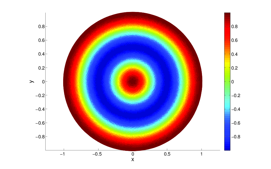 |
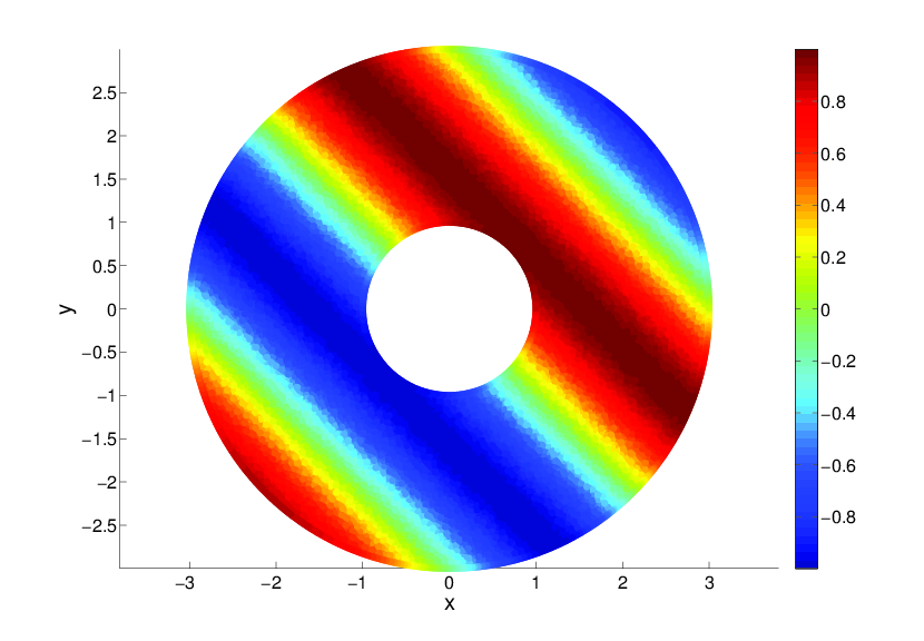 |
| (a) | (b) |
The coefficient of the equation in (4.1) is
| (4.2) |
both in the unit disk and annulus. The Neumann boundary condition is enforced in unit disk and we consider the Dirichlet boundary condition in the annulus.
Table 1 list the error of the point integral method as the number of points grows. This result clearly shows the convergence of the point integral method. The convergence rate in error is approximately .
| 684 | 2610 | 10191 | 40296 | |
|---|---|---|---|---|
| disk | 0.364597 | 0.214960 | 0.111961 | 0.056028 |
| annulus | 0.036760 | 0.012227 | 0.005557 | 0.003542 |
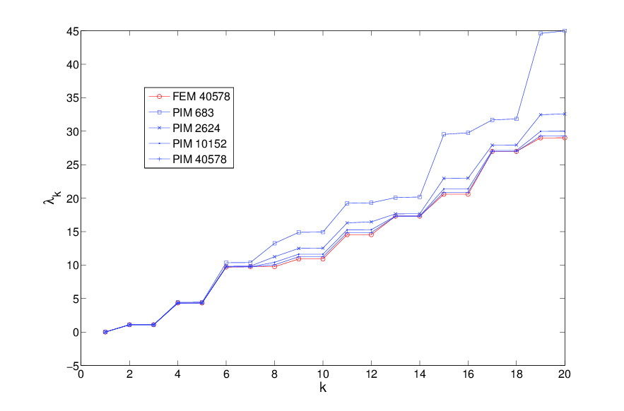
The eigenvalue problem with homogeneous Neumann boundary condition is also solved in the annulus.
and the coefficient is given in (4.2).
The first 20 eigenvalues are plotted in Figure 2. The eigenvalues given by finite element method in the finest mesh is used as the true solution. Our result shows that the eigenvalue computed in the point integral method also converge.
Example 2
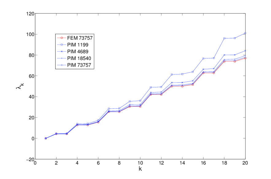
Now, we solve equation (4.1) with Neumann condition and Dirichlet condition on a curved surface in . Let be a cap on the unit sphere, whose height is and the cap angle is , as shown in Figure 3. The coefficient of the equation is also given in (4.2).
We set the ground truth to be , where is the coordinate in .
 |
The errors of the point integral method are listed in Table 2. The convergence rate for both boundary value problems are .
| 1199 | 4689 | 18540 | 73757 | |
|---|---|---|---|---|
| Neumann | 0.036779 | 0.015355 | 0.007479 | 0.003189 |
| Dirichlet | 0.007238 | 0.001921 | 0.001278 | 0.000750 |
The first 20 eigenvalues are also computed for homogeneous Neumann condition as shown in Figure 4. As the number of points increases, the eigenvalues given by PIM converge to those computed by FEM, which suggests the convergence of the point integral method.
Example 3
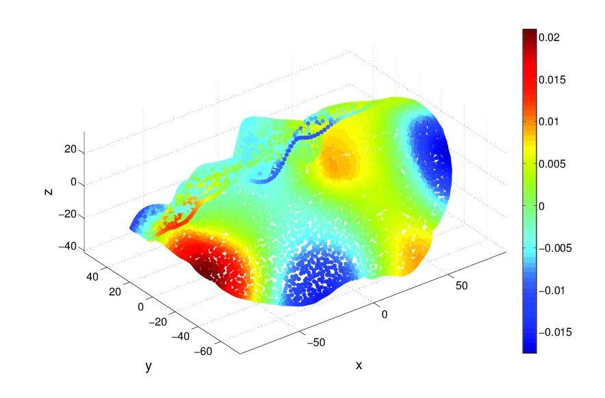
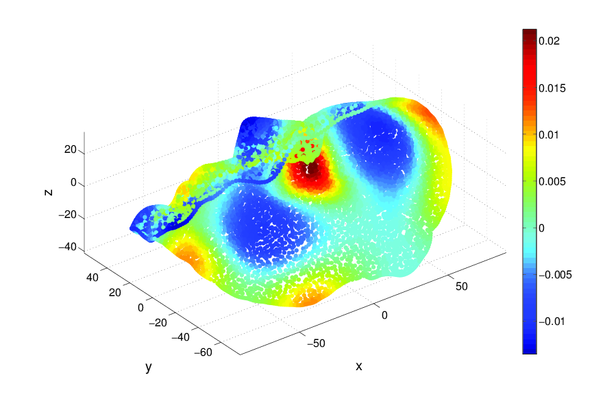
In this example, we consider a more complex surface, a human face called ”Alex”. The surface is sampled by 10597 points (Figure 5) and the analytic form of the surface is not known. The coefficient of the equation in (4.1) is
where .
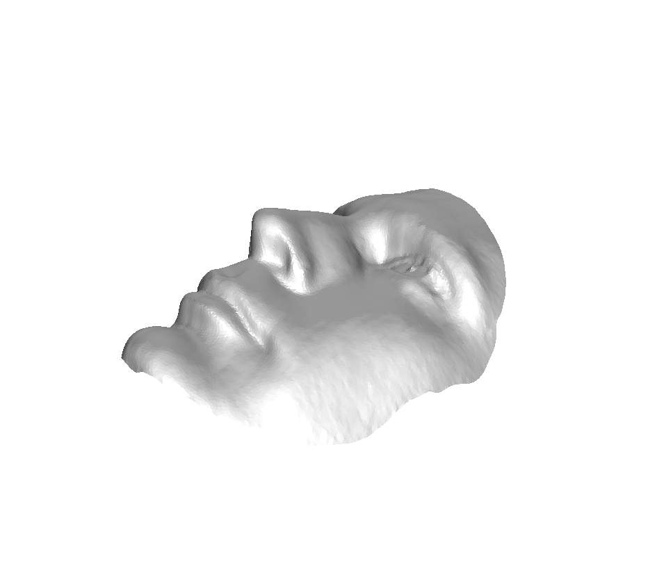 |
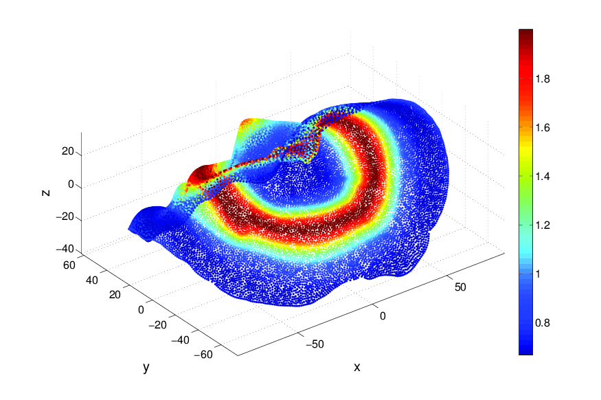 |
In this example, we solve the eigenvalue problem of the isotropic elliptic operator. Several eigenfunctions computed by the point integral method are shown in Figure 6.
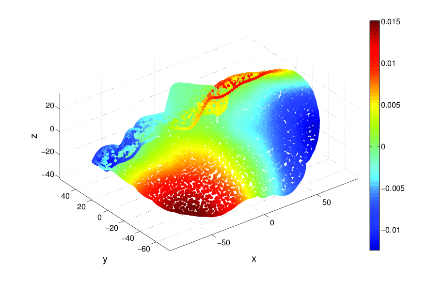 |
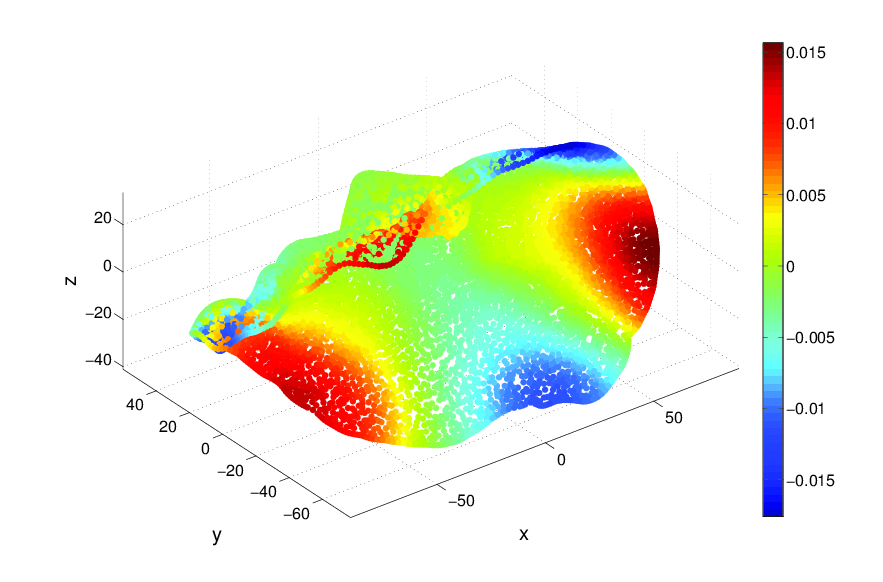 |
 |
 |
From the examples in 2D surfaces, we see that PIM solves isotropic elliptic equations with Neumann and Dirichlet boundary very well. Moreover, the convergence rate is higher than that obtained in the convergence analysis. The point integral method is applicable to point cloud in high dimensional space, not only on the 2D surfaces. Next, we will show a high dimensional example.
4.2 Nonlocal Total Variation Extension
In this example, we consider an extension on point cloud. The point cloud is constructed by using the patches of a image, which is shown in Figure 7(a). The original image is subsampled and only retain 10% of the pixels at random. The subsampled image is shown in Figure 7(b). One classical problem in image processing is to recover the image from the subsampled image. Here, rather than give an image reconstruction method, we only use this example to demonstrate the performance of the point integral method for isotropic elliptic equations.
In this example, the point cloud consists of the patches of the original image. For each pixel in the image , we extract a patch around it of size which is denoted as , where is the original image. Totally, we get patches and each patch is . The collection of all the patches give a point cloud in . Denote this point cloud as . The image is actually corresponding a function on the point cloud with , is the value of image at pixel . Corresponding to the subsampled image, the value of function is only known in the patches around the sampled pixels. The collection of all these patches is denoted as .
Recently, manifold model attracts many attentions in image processing [30]. In manifold model, the point cloud is assumed to be a sample of an underlying manifold, which is called patch manifold. The total variation is used as a regularization to reconstruct the image. The main idea is to minimize the total variation in the patch manifold, i.e.,
| (4.3) |
The variation approach tells us that the optimal solution of (4.3) is given by solving following PDE,
with the Dirichlet type boundary condition
One natural method to solve above PDE is an iterative scheme,
| (4.4) |
In each step, we need to solve an isotropic elliptic equation.
Here, the gradient is computed by using an integral approximation also.
. In the computation, to avoid degenerate of the ellipticity, we regularize the coefficient by adding a small constant in the denominator, i.e., replace by in (4.4) with . The point cloud is assumed to be uniformly distributed, so the volume weight is uniform. The kernel function is Gaussian function. In this example, we use the integral approximation (2.17) with adaptive , where is the radius of 20 nearest neighbors of .
 |
 |
| (a) | (b) |
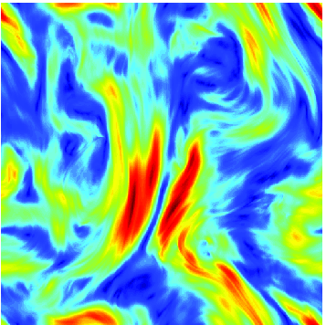
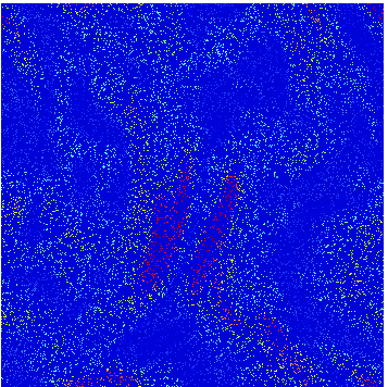
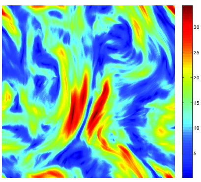
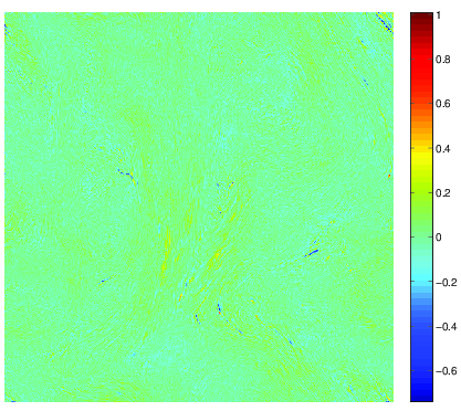
Figure 8(a) shows the image reconstructed by extension and Figure 8(b) gives the difference between the original image, Figure 7(a) and the reconstructed image Figure 8(a). As we can see, extension gives very good reconstruction. This result shows that the point integral method solve the isotropic elliptic equation very well on point cloud.
 |
 |
| (a) | (b) |
5 Conclusion
In this paper, we generalize the point integral method to solve the isotropic elliptic equation. The point integral method is very easy to implement on point cloud, since it only needs the point cloud without any extra information. Moreover, it also has very good theoretical property. The coercivity of the original elliptic operator is partially preserved in the point integral method. Based on this property, the convergence is proved.
One important implication is the spectral convergence of the point integral method on random samples. Suppose the points are obtained by sampling a manifold according to some probability distribution . In the point integral method, the eigenvalue problem
| (5.3) |
is discretized as
| (5.4) |
This discretization is closely related with the normalized graph laplacian. Based on the theoretical results in this paper, it can be proved that the spectra of (5.4) converges to the spectra of (5.3) as the number of sample points goes to infinity.
The other interesting problem is how to generalize the point integral method to anisotropic elliptic equation. On this problem, we already get some results. They are going to be reported in the subsequent paper.
References
- [1] F. Andreu, J. M. Mazon, J. D. Rossi, and J. Toledo. Nonlocal Diffusion Problems. Math. Surveys Monogr. 165, AMS, Providence, RI, 2010.
- [2] R. Barreira, C. Elliott, and A. Madzvamuse. Modelling and simulations of multi-component lipid membranes and open membranes via diffuse interface approaches. J. Math. Biol., 56:347–371, 2008.
- [3] R. Barreira, C. Elliott, and A. Madzvamuse. The surface finite element method for pattern formation on evolving biological surfaces. J. Math. Biol., 63:1095–1119, 2011.
- [4] M. Belkin and P. Niyogi. Laplacian eigenmaps for dimensionality reduction and data representation. Neural Computation, 15(6):1373–1396, 2003.
- [5] M. Belkin and P. Niyogi. Towards a theoretical foundation for laplacian-based manifold methods. In COLT, pages 486–500, 2005.
- [6] M. Belkin and P. Niyogi. Convergence of laplacian eigenmaps. preprint, short version NIPS 2008, 2008.
- [7] M. Belkin, J. Sun, and Y. Wang. Constructing laplace operator from point clouds in rd. In SODA ’09: Proceedings of the Nineteenth Annual ACM -SIAM Symposium on Discrete Algorithms, pages 1031–1040, Philadelphia, PA, USA, 2009. Society for Industrial and Applied Mathematics.
- [8] M. Bertalmio, L.-T. Cheng, S. Osher, and G. Sapiro. Variational problems and partial differential equations on implicit surfaces. Journal of Computational Physics, 174(2):759 – 780, 2001.
- [9] J. W. Cahn, P. Fife, and O. Penrose. A phase-field model for diffusion-induced grain-boundary motion. Ann. Statist., 36(2):555–586, 2008.
- [10] F. R. K. Chung. Spectral Graph Theory. American Mathematical Society, 1997.
- [11] R. R. Coifman, S. Lafon, A. B. Lee, M. Maggioni, F. Warner, and S. Zucker. Geometric diffusions as a tool for harmonic analysis and structure definition of data: Diffusion maps. In Proceedings of the National Academy of Sciences, pages 7426–7431, 2005.
- [12] Q. Du, M. Gunzburger, R. B. Lehoucq, and K. Zhou. Analysis and approximation of nonlocal diffusion problems with volume constraints. SIAM Review, 54:667–696, 2012.
- [13] Q. Du, M. Gunzburger, R. B. Lehoucq, and K. Zhou. A nonlocal vector calculus, nonlocal volume-constrained problems, and nonlocal balance laws. Math. Models Methods Appl. Sci., 23:493–540, 2013.
- [14] Q. Du, L. Ju, L. Tian, and K. Zhou. A posteriori error analysis of finite element method for linear nonlocal diffusion and peridynamic models. Math. Comp., 82:1889–1922, 2013.
- [15] Q. Du, T. Li, and X. Zhao. A convergent adaptive finite element algorithm for nonlocal diffusion and peridynamic models. SIAM J. Numer. Anal., 51:1211–1234, 2013.
- [16] G. Dziuk and C. M. Elliott. Finite element methods for surface pdes. Acta Numerica, 22:289–396, 2013.
- [17] C. Eilks and C. M. Elliott. Numerical simulation of dealloying by surface dissolution via the evolving surface finite element method. J. Comput. Phys., 227:9727–9741, 2008.
- [18] C. M. Elliott and B. Stinner. Modeling and computation of two phase geometric biomem- branes using surface finite elements. J. Comput. Phys., 229:6585–6612, 2010.
- [19] S. Ganesan and L. Tobiska. A coupled arbitrary lagrangian eulerian and lagrangian method for computation of free-surface flows with insoluble surfactants. J. Comput. Phys., 228:2859–2873, 2009.
- [20] M. Hein, J.-Y. Audibert, and U. von Luxburg. From graphs to manifolds - weak and strong pointwise consistency of graph laplacians. In Proceedings of the 18th Annual Conference on Learning Theory, COLT’05, pages 470–485, Berlin, Heidelberg, 2005. Springer-Verlag.
- [21] A. J. James and J. Lowengrub. A surfactant-conserving volume-of-fluid method for interfacial flows with insoluble surfactant. J. Comput. Phys., 201:685–722, 2004.
- [22] S. Lafon. Diffusion Maps and Geodesic Harmonics. PhD thesis, 2004.
- [23] R. Lai, J. Liang, and H. Zhao. A local mesh method for solving pdes on point clouds. Inverse Problem and Imaging, 7:737–755, 2013.
- [24] S. Leung, J. Lowengrub, and H. Zhao. A grid based particle method for solving partial differential equations on evolving surfaces and modeling high order geometrical motion. J. Comput. Phys., 230(7):2540–2561, 2011.
- [25] S. Leung and H. Zhao. A grid based particle method for moving interface problems. J. Comput. Phys., 228(8):2993–3024, 2009.
- [26] Z. Li, Z. Shi, and J. Sun. Point integral method for solving poisson-type equations on manifolds from point clouds with convergence guarantees. arXiv:1409.2623.
- [27] J. Liang and H. Zhao. Solving partial differential equations on point clouds. SIAM Journal of Scientific Computing, 35:1461–1486, 2013.
- [28] C. Macdonald and S. Ruuth. The implicit closest point method for the numerical so- lution of partial differential equations on surfaces. SIAM J. Sci. Comput., 31(6):4330–4350, 2009.
- [29] M. P. Neilson, J. A. Mackenzie, S. D. Webb, and R. H. Insall. Modelling cell movement and chemotaxis using pseudopod-based feedback. SIAM J. Sci. Comput., 33:1035–1057, 2011.
- [30] S. Osher, Z. Shi, and W. Zhu. Low dimensional manifold model for image processing. Technical report, UCLA, CAM-report 16-04.
- [31] G. Peyré. Manifold models for signals and images. Computer Vision and Image Understanding, 113:248–260, 2009.
- [32] S. Ruuth and B. Merriman. A simple embedding method for solving partial differ- ential equations on surfaces. J. Comput. Phys., 227(3):1943–1961, 2008.
- [33] Z. Shi and J. Sun. Convergence of the point integral method for the poisson equation on manifolds i: the neumann boundary. arXiv:1403.2141.
- [34] Z. Shi and J. Sun. Convergence of the point integral method for the poisson equation on manifolds ii: the dirichlet boundary. arXiv:1312.4424.
- [35] A. Singer. From graph to manifold Laplacian: The convergence rate. Applied and Computational Harmonic Analysis, 21(1):128–134, July 2006.
- [36] A. Singer and H. tieng Wu. Spectral convergence of the connection laplacian from random samples. arXiv:1306.1587.
- [37] J. Xu and H. Zhao. An eulerian formulation for solving partial differential equations along a moving interface. J. Sci. Comput., 19:573–594, 2003.
- [38] K. Zhou and Q. Du. Mathematical and numerical analysis of linear peridynamic models with nonlocal boundary conditions. SIAM J. Numer. Anal., 48:1759–1780, 2010.