On the Cauchy problem and the black solitons of a singularly perturbed Gross-Pitaevskii equation

Abstract.

We consider the one-dimensional Gross-Pitaevskii equation perturbed by a Dirac potential. Using a fine analysis of the properties of the linear propagator, we study the well-posedness of the Cauchy Problem in the energy space of functions with modulus 1 at infinity. Then we show the persistence of the stationary black soliton of the unperturbed problem as a solution. We also prove the existence of another branch of non-trivial stationary waves. Depending on the attractive or repulsive nature of the Dirac perturbation and of the type of stationary solutions, we prove orbital stability via a variational approach, or linear instability via a bifurcation argument.

1. Introduction

We consider the one-dimensional singularly perturbed Gross-Pitaevskii equation

$$iu_{t}+u_{xx}-\gamma\delta u+(1-|u|^{2})u=0,$$ (1.1)

with the boundary condition

$$|u(t,x)|\to 1,\quad\text{as}\quad|x|\to+\infty.$$ (1.2)

Here, $u:\mathbb{R}\times\mathbb{R}\to\mathbb{C}$, $\gamma\in\mathbb{R}$, $\delta$ is the Dirac distribution at $0$ and the indices denote the derivatives.

The Gross-Pitaevskii equation is a defocusing nonlinear Schrödinger equation with non-standard boundary conditions. It has numerous applications in physics, in particular in nonlinear optics or for Bose-Einstein condensates. Since we assume that $|u|\to 1$ at infinity, a rich nonlinear dynamics is possible. In particular, there exist solutions of (1.1) either stationary or propagating a fixed profile: the dark and grey solitons.

Perturbations of nonlinear Schrödinger equations with one or more Dirac distributions appear in different contexts in Physics and Mathematics.

In nonlinear optics, when polarization of light and birefringence are taken into account in the modeling of optical fibers, the resulting model is a system of coupled nonlinear Schrödinger equations, see [8]. In the study of the soliton-soliton collisions (see e.g. [25, 43]), if one of the component is very narrow, then its effect on the other via the coupling can be approximated by the Dirac distribution (see [18] and the references therein). The mathematical phenomena related to the interaction of a soliton with the Dirac perturbation have been studied in depth, first in the groundlaying work by Goodman, Holmes and Weinstein [36] and then in a series of papers by Datchev, Holmer, Marzuola and/or Zworski [24, 40, 41, 42].

Dirac distributions also naturally appear for nonlinear Schrödinger equations on graphs. The motivation comes from nanotechnology where networks of quantum wires are modeled by nonlinear Schrödinger equations on graphs with the Laplacian on the edges and Kirchoff transmission conditions at the vertices. The equation (1.1) constitutes the simplest example of a nonlinear Schrödinger equation posed on a graph consisting of only one vertex and two edges. An introduction to nonlinear Schrödinger equations on graphs is provided by Noja in [48].

The mathematical study of singularly perturbed nonlinear Schrödinger equations started only a few years ago and is currently in very active development. Several lines of investigation have been followed. One problem is to understand the effect of the perturbation on the dispersive nature of the equation. Outstanding progresses have been made recently in this direction by Banica and Ignat [11, 12]. Another challenge is to analyse the solitons and their stability. After the pioneering work of Fukuizumi and co. [27, 28, 45], the analysis of solitons for nonlinear Schrödinger equations on graphs has known a tremendous development under the impulsion of Adami and co. [1, 2, 3, 4, 5, 6]. Surprising phenomena appear, e.g. bistability in the recent work of Genoud, Malomed and Weishäupl [31]. Let us mention also the recent study of the scattering problem by Banica and Visciglia [13].

To our knowledge, our work is the first one where the singularly perturbed Gross-Pitaevskii equation (1.1) with the non-standard boundary conditions (1.2) is considered. We are interested by the Cauchy problem for (1.1) and by the existence and stability of stationary solutions. As detailed below, two main difficulties arise. First, due to the non-standard boundary conditions, the natural energy space is not a vector space and we have to rethink entirely the strategy to solve the Cauchy problem. Second, the presence of the Dirac perturbation generates subtle modifications on the stationary solutions of the equation, thus its treatment requires a fine analysis, in particular for the spectral part of the study.

Before presenting our results, we give some preliminaries on the structure of (1.1). At least formally, we have the conservation of the energy $E_{\gamma}$ defined by

$$E_{\gamma}(u)=\frac{1}{2}\lVert u^{\prime}\rVert_{L^{2}}^{2}+\frac{\gamma}{2}|u(0)|^{2}+\frac{1}{4}\int_{\mathbb{R}}(1-|u|^{2})^{2}\,dx,$$

where ^′ denotes the derivative with respect to the variable $x$. Then the equation (1.1) can be rewritten into the Hamiltonian form

$$iu_{t}=\partial E_{\gamma}(u).$$

This energy is defined in the energy space

$$\mathcal{E}:=\left\{v\in H^{1}_{\mathrm{loc}}(\mathbb{R}):\;v^{\prime}\in L^{2}(\mathbb{R}),\,(1-|v|^{2})\in L^{2}(\mathbb{R})\right\}.$$

Unfortunately $\mathcal{E}$ is not a vector space and this yields several difficulties in the analysis. We will endow $\mathcal{E}$ with the structure of a complete metric space. Several choices are possible for the distance (see e.g. the discussion in [33]). In this work, we have used the two distances $d_{0}$ and $d_{\infty}$ defined as follows. For $u,v\in{\mathcal{E}}$ we set

$$d_{0}(u,v) =\left\|u^{\prime}-v^{\prime}\right\|_{L^{2}}+\lvert u(0)-v(0)\rvert+\left\|\lvert u\rvert^{2}-\lvert v\rvert^{2}\right\|_{L^{2}},$$ (1.3)

$$d_{\infty}(u,v) =\left\|u^{\prime}-v^{\prime}\right\|_{L^{2}}+\left\|u-v\right\|_{L^{\infty}}+\left\|\lvert u\rvert^{2}-\lvert v\rvert^{2}\right\|_{L^{2}}.$$ (1.4)

The size of $u$ in ${\mathcal{E}}$ will be measured with the quantity

$$\lvert u\rvert_{\mathcal{E}}^{2}=E_{0}(u)=\frac{1}{2}\left\|u^{\prime}\right\|^{2}_{L^{2}}+\frac{1}{4}\int_{\mathbb{R}}(1-|u|^{2})^{2}\,dx.$$ (1.5)

Note that we have used $E_{0}$ instead of $E_{\gamma}$ in the definition of $\lvert u\rvert_{\mathcal{E}}$ because the Dirac perturbation is not encoded in the energy space. Notice moreover that $E_{\gamma}(u)$ may be negative when $\gamma$ is negative.

1.1. The Cauchy Problem

Our first main result concerns the well-posedness of the Cauchy Problem for (1.1) in the energy space $\mathcal{E}$.

A lot of research has been devoted in the last decades to the study of the Cauchy Problem for various dispersive PDE and one would expect that a classical-looking equation like (1.1) is already covered by existing results. This is however not the case, as most of the works on dispersive PDE deal with well-posedness in vector function spaces for localized or periodic functions. Because of the condition $|u|\to 1$ at infinity, (1.1) does not fall into that category, and the Cauchy Theory for non-vector function spaces like ${\mathcal{E}}$ is still at its early stages of development (see e.g. [29, 33, 34]). Another difficulty arising when dealing specifically with (1.1) is the effect of the Dirac perturbation, which causes a loss of regularity at $x=0$ for the solution.

Our result is the following.

Theorem 1.1 (The Cauchy Problem).

Let $\gamma\in\mathbb{R}$. Then for any $u_{0}\in{\mathcal{E}}$ the problem (1.1) has a unique, global, continuous (for $d_{\infty}$ and hence $d_{0}$) solution $u:\mathbb{R}\to{\mathcal{E}}$ with $u(0)=u_{0}$. Moreover, the following properties are satisfied.

• Energy conservation: For all $t\in\mathbb{R}$ we have

  $$E_{\gamma}(u(t))=E_{\gamma}(u_{0}).$$

• Continuity with respect to the initial condition: For $R>0$ and $T>0$ there exists $C>0$ such that for $u_{0},\tilde{u}_{0}\in{\mathcal{E}}$ with $\lvert u_{0}\rvert_{\mathcal{E}}\leqslant R$ and $\lvert\tilde{u}_{0}\rvert_{\mathcal{E}}\leqslant R$ the corresponding solutions $u$ and $\tilde{u}$ satisfy

  $$\forall t\in(-T,T),\quad d_{\infty}\big{(}u(t),\tilde{u}(t)\big{)}\leqslant Cd_{\infty}(u_{0},\tilde{u}_{0}).$$

The proof of Theorem 1.1 is based on a fixed point argument. Several steps are necessary.

A main task is to acquire a good understanding on the linear propagation. We denote by $H_{\gamma}$ the unbounded self-adjoint operator rigorously defined from the formal expression $-\partial_{xx}+\gamma\delta$ (see Section 2.2):

$$\begin{cases}H_{\gamma}=-\displaystyle\frac{d^{2}}{dx^{2}},\\ D(H_{\gamma})=\left\{u\in H^{1}(\mathbb{R})\cap H^{2}(\mathbb{R}\setminus\{0\})\,:\,u^{\prime}(0^{+})-u^{\prime}(0^{-})=\gamma u(0)\right\}.\end{cases}$$

Note that $H_{\gamma}$ differs from the usual second order derivative operator only by the jump condition:

$$\partial_{x}u(0^{+})-\partial_{x}u(0^{-})=\gamma u(0).$$ (1.6)

We start by giving an explicit characterization of the linear group $e^{-itH_{\gamma}}$. Precisely, we decompose the linear group $e^{-itH_{\gamma}}$ in a regular part containing the free propagator $e^{-itH_{0}}$ and a singular part $\Gamma(t)$:

$$e^{-itH_{\gamma}}=e^{-itH_{0}}+\Gamma(t),$$

and we give an explicit expression for the kernel of $\Gamma(t)$.

As expected, the treatment of the free linear evolution does not cause any trouble, and the tricky part is to deal with $\Gamma(t)$. In particular, when $\gamma<0$, the kernel of $\Gamma(t)$ is rather hard to handle, and we have to find a clever way to decompose it into two parts that are treatable separately (see the decomposition in Lemma 3.2). This decomposition is crucially involved in the rest of the study of the linear evolution. Whereas the explicit formula for the kernel was previously derived in the literature, the decomposition lemma is a new tool to deal with the propagator $e^{-itH_{\gamma}}$.

With the explicit formula for the kernel of the propagator and the decomposition lemma at our disposal, we are equipped for the study of the propagator $e^{-itH_{\gamma}}$. We first prove that it defines a continuous map on $H^{1}(\mathbb{R})$. It is clear if $\gamma=0$ since $H_{0}=-\partial_{xx}$ commutes with derivatives, but it is no longer the case when $\gamma\neq 0$. Then we extend $e^{-itH_{\gamma}}$ to a map on the energy space ${\mathcal{E}}$. This map will inherit most of the nice properties of the unitary group on $L^{2}(\mathbb{R})$. Finally, we prove that for $u_{0}\in{\mathcal{E}}$ the map $t\mapsto e^{-itH_{\gamma}}u_{0}-u_{0}$ is continuous with values in $H^{1}(\mathbb{R})$. In other words, it sends functions with non-zero boundary data at infinity to localized functions. That is a central point in our analysis.

After the study of the linear propagator, we are ready to tackle the analysis of the Cauchy Problem. We rewrite the problem (1.1) in terms of a Duhamel formula, to which we will apply Banach fixed point theorem to prove the local well-posedness.

The last step consists in proving the conservation of the energy. As usual (see e.g. [19]), we first consider a dense subset of more regular initial data, for which (1.1) has a strong solution. However, the singular nature of the Dirac perturbation prevents us from working with functions regular at $0$. Thus, we have constructed the space $X_{\gamma}^{2}$ of functions which have locally the $H^{2}(\mathbb{R})$ regularity and satisfy at 0 the jump condition (1.6) generated by the Dirac perturbation. We prove the conservation of the energy for such an initial condition $u_{0}$ and then, by density, for any $u_{0}\in{\mathcal{E}}$. Global existence is then a consequence of energy conservation.

1.2. The Black Solitons

When $\gamma=0$, (1.1) admits traveling waves, i.e. solutions of the form $\kappa_{c}(x-ct)$. In this case, a traveling wave of finite energy is either a constant of modulus $1$ or, for $|c|<\sqrt{2}$ and up to phase shifts or translations, it has a non-trivial profile given by an explicit formula.

The nontrivial traveling waves have been the subject of a thorough investigation in the recent years. When $c\neq 0$, they are often called grey solitons, a terminology which stems from nonlinear optics (such solitons appear grey in the experiments). For $c\neq 0$, orbital stability was proved via the Grillakis-Shatah-Strauss Theory [38, 39] by Lin [46] and later revisited by Bethuel, Gravejat and Saut [14] via the variational method introduced by Cazenave and Lions [20]. When $c=0$, the traveling wave becomes a stationary wave and is now called a black soliton. The study of orbital stability is much trickier when $c=0$, due to the fact that the solution vanishes, and it is no longer possible to make use of the so-called hydrodynamical formulation of the Gross-Pitaevskii equation (see e.g. [14] for details). Nevertheless orbital stability of the black soliton was proved via variational methods by Bethuel, Gravejat, Saut and Smets [15] and via the inverse scattering transform by Gérard and Zhang [35] (see also [26] for an earlier result and numerical simulations). Recently, Bethuel, Gravejat and Smets proved the orbital stability of a chain of solitons of the Gross-Pitaevskii equation [16] as well as asymptotic stability of the grey solitons [17] and of the black soliton [37]. Existence and stability of traveling waves with a non-zero background for equations of type (1.1) with a general nonlinearity was also studied by Chiron [22, 23].

When $\gamma\neq 0$, the Dirac perturbation breaks the translation invariance and traveling waves do not exist anymore. However, stationary solutions $u(t,x)\equiv u(x)$ solving the ordinary differential equation

$$u^{\prime\prime}-\gamma\delta u+(1-|u|^{2})u=0$$ (1.7)

are still expected. In fact, the black soliton $\kappa_{0}$ is still a solution to (1.1) when $\gamma\neq 0$, and other branches of nontrivial solutions bifurcate from the constants of modulus $1$. Precisely (see Proposition 5.1) the set of finite-energy solutions to (1.7) is

$$\left\{e^{i\theta}\kappa,e^{i\theta}b_{\gamma}\ :\ \theta\in\mathbb{R}\right\} \text{ if }\gamma>0,$$

$$\left\{e^{i\theta}\kappa,e^{i\theta}b_{\gamma},e^{i\theta}\tilde{b}_{\gamma}\ :\ \theta\in\mathbb{R}\right\} \text{ if }\gamma<0,$$

where (see also Figure 1)

$$\kappa(x):=\tanh\left(\frac{x}{\sqrt{2}}\right),\quad b_{\gamma}(x):=\tanh\left(\frac{|x|-c_{\gamma}}{\sqrt{2}}\right),\quad\tilde{b}_{\gamma}(x):=\coth\left(\frac{|x|+c_{\gamma}}{\sqrt{2}}\right),$$

for $c_{\gamma}:=\frac{1}{\sqrt{2}}\sinh^{-1}\left(-\frac{2\sqrt{2}}{\gamma}\right)$. This existence result is obtained using ordinary differential equations techniques. The analysis of (1.7) is classical when $\gamma=0$ and the difficulty when $\gamma\neq 0$ is to deal with the jump condition (1.6) induced by the Dirac perturbation.

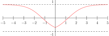
Figure 1. Top Left: The stationary state $\kappa=\kappa_{0}=\tanh\left(\frac{x}{\sqrt{2}}\right)$.
Top Right: The stationary state $\tilde{b}_{\gamma}(x):=\coth\left(\frac{|x|+c_{\gamma}}{\sqrt{2}}\right),$ $\gamma=-1$.
Bottom: The stationary state $b_{\gamma}$ for $\gamma=-1$ and $\gamma=1$.

The next step in the study of stationary solutions to (1.1) is to understand their stability. To this aim, and when possible, we give a variational characterization of the stationary solutions. When $\gamma=0$, the traveling waves can be characterized as minimizers of the energy on a fixed momentum constraint. This is a non-trivial result due to difficulties in the definition of the momentum (see [14, 15]). We will show in our next result that, depending on the sign of $\gamma$, either $\tilde{b}_{\gamma}$ or $b_{\gamma}$ can be characterized as minimizers. The minimization problem turns out to be simpler than when $\gamma=0$, and the stationary solutions are in fact global minimizers of the energy without constraint.

The minimization result is the following.

Proposition 1.2 (Variational Characterization).

Let $\gamma\in\mathbb{R}\setminus\{0\}$. Then we have

$$m_{\gamma}:=\inf\{E_{\gamma}(v):v\in{\mathcal{E}}\}>-\infty.$$

Moreover the infimum is achieved at solutions to (1.7). Precisely, define

$$\mathcal{G}_{\gamma}:=\{v\in\mathcal{E},\quad E_{\gamma}(v)=m_{\gamma}\}.$$

Then the following assertions hold.

• If $\gamma>0$, then $\mathcal{G}_{\gamma}=\{e^{i\theta}b_{\gamma},\theta\in\mathbb{R}\}$,

• If $\gamma<0$, then $\mathcal{G}_{\gamma}=\{e^{i\theta}\tilde{b}_{\gamma},\theta\in\mathbb{R}\}$.

In addition, any minimizing sequence $(u_{n})\subset\mathcal{E}$ such that $E_{\gamma}(u_{n})\to m_{\gamma}$ verifies, up to a subsequence,

$$d_{0}(u_{n},\mathcal{G}_{\gamma})\to 0.$$

In the cases covered by Proposition 1.2, stability will be a corollary of the variational characterization of the stationary states as global minimizers of the energy. Let us recall that we say that the set $\mathcal{G}_{\gamma}\subset\mathcal{E}$ is stable if for any $\varepsilon>0$ there exists $\delta>0$ such that for any $u_{0}\in\mathcal{E}$ with

$$d_{0}(u_{0},\mathcal{G}_{\gamma})\leqslant\delta,$$

the solution $u$ of (1.1) with $u(0)=u_{0}$ is global and verifies

$$\sup_{t\in\mathbb{R}}d_{0}(u(t),\mathcal{G}_{\gamma})\leqslant\varepsilon.$$

When the stationary solutions are not minimizers of the energy, we expect them to be all unstable. In this paper, we treat the case $\gamma>0$ and we show that $\kappa$ is linearly unstable.

Linear instability means that the operator arising in the linearization of (1.1) around $\kappa$ (see e.g. [21]) admits an eigenvalue with negative real part. Precisely, consider the linearization of (1.1) around the kink stationary solution $\kappa(x)$. For $u$ solution of (1.1) we write $u=\kappa+\eta$. The perturbation $\eta$ verifies

$$\eta_{t}+L\eta+N(\eta)=0,$$ (1.8)

where the linear and nonlinear parts are given by

$$L\eta =-i(\partial_{xx}\eta-\gamma\delta\eta+(1-\kappa^{2})\eta-2\kappa^{2}\mathcal{R}\!\mathpzc{e}(\eta)),$$ (1.9)

$$N(\eta) =-i(-2\kappa\mathcal{R}\!\mathpzc{e}(\eta)\eta-|\eta|^{2}(\kappa+\eta)).$$

The kink $\kappa$ is said to be linearly unstable if $0$ is an unstable solution of the linear equation

$$\eta_{t}+L\eta=0.$$

This is in particular the case if $L$ has an eigenvalue $\lambda$ with $\mathcal{R}\!\mathpzc{e}(\lambda)<0$. Indeed, such eigenvalue generates an exponential growth for the corresponding solution of the linear problem. It is expected that this linear exponential growth translates into nonlinear instability, as in the theory of Grillakis, Shatah and Strauss [39], see [32] for a rigorous proof in the case of a nonlinear Schrödinger equation.

The stability/instability result is the following.

Theorem 1.3 (Stability/Instability).

The following assertions hold.

• (Stability) Let $\gamma\neq 0$. Then the set $\mathcal{G}_{\gamma}$ is stable under the flow of (1.1).

• (Instability) Let $\gamma>0$. Then the kink $\kappa$ is linearly unstable.

Remark 1.4.

In the stability result, a solution starting close to a stationary wave will always remain close, up to a phase parameter which may vary in time. This type of stability is usually called orbital stability (see [20] for an early result on orbital stability and [19, Chapter 8] for a discussion of the orbital nature of stability).

Remark 1.5.

It is interesting to note that if we define $m_{\gamma,\mathrm{rad}}$ (resp. $m_{\gamma,\mathrm{odd}}$) to be the minimum of $E_{\gamma}(v)$ with $v\in{\mathcal{E}}$, $v$ even (resp. odd), then for any $\gamma\in\mathbb{R}$ we have

$$\mathcal{G}_{\gamma,\mathrm{rad}} =\{v\in\mathcal{E},v\text{ even},E_{\gamma}(v)=m_{\gamma,\mathrm{rad}}\}=\{e^{i\theta}b_{\gamma},\theta\in\mathbb{R}\},\quad\text{if }\gamma>0$$

$$\mathcal{G}_{\gamma,\mathrm{rad}} =\{v\in\mathcal{E},v\text{ even},E_{\gamma}(v)=m_{\gamma,\mathrm{rad}}\}=\{e^{i\theta}\tilde{b}_{\gamma},\theta\in\mathbb{R}\},\quad\text{if }\gamma<0$$

$$\mathcal{G}_{\gamma,\mathrm{odd}} =\{v\in\mathcal{E},v\text{ odd},E_{\gamma}(v)=m_{\gamma,\mathrm{odd}}\}=\{e^{i\theta}\kappa,\theta\in\mathbb{R}\}.$$

In particular, the kink $\kappa$ is always stable with respect to odd perturbations.

Remark 1.6.

Perturbations measured in $d_{0}$ allow for overall phase changes. It is an interesting question whether a single minimizer can be stable against a class of more localized perturbations (without phase change)? In [35], orbital stability of the kink was obtained without phase change, for a class of polynomially decreasing perturbations. However, their method does not apply in our setting.

As already said, part (i) (Stability) in Theorem 1.3 is a corollary of Proposition 1.2. The proof of part (ii) (Instability) of Theorem 1.3 relies on a perturbative analysis partly inspired by [45]. We first convert $L$ into a new operator $\mathcal{L}$ by separating the real and imaginary parts. The operator $\mathcal{L}$ is of the form

$$\mathcal{L}=\begin{pmatrix}0&-L_{-}^{\gamma}\\ L^{\gamma}_{+}&0\end{pmatrix},$$

where $L_{+}^{\gamma}$ and $L_{-}^{\gamma}$ are selfadjoint operators whose spectra are well known when $\gamma=0$. Then we use the continuity of these spectra with respect to $\gamma$ to obtain information on the general case. For instance, $0$ is a simple and isolated eigenvalue of $L_{+}^{0}$. For $\gamma\neq 0$, $|\gamma|\ll 1$, this eigenvalue moves on one side or the other of the real line, depending on the sign of $\gamma$. Then we show that when $\gamma\neq 0$ the kernel is always trivial, which implies that the number of negative eigenvalues is constant for $\gamma\in(-\infty,0)$ and for $\gamma\in(0,+\infty)$. With this kind of information on the spectrum of $L_{\pm}^{\gamma}$, we can prove that $\mathcal{L}$ has a real negative eigenvalue, which is also an eigenvalue for $L$.

The rest of the paper is divided as follows. In Section 2 we analyse the structure of the functional spaces involved in the analysis, in particular the energy space ${\mathcal{E}}$. Section 3 is devoted to the study of the linear propagator. This provides the necessary tools to prove the well-posedness of the Cauchy Problem in Section 4. In Section 5 we prove the existence and variational characterizations of the stationary solutions, and we analyse their stability/instability in Section 6.

Acknowledgment.

The authors are grateful to Masahito Ohta for pointing them out the existence of the family of $\coth$ based bound states. They are also grateful to the unknown referee for helpful comments.

Notation.

The space $L^{2}(\mathbb{R})$ will be endowed with the real scalar product

$$\left<u,v\right>_{L^{2}}=\mathcal{R}\!\mathpzc{e}\int_{\mathbb{R}}u\bar{v}dx.$$

The homogeneous Sobolev space $\dot{H}^{1}(\mathbb{R})$ is defined by

$$\dot{H}^{1}(\mathbb{R})=\{u\in H^{1}_{\mathrm{loc}}(\mathbb{R})\,:\,u^{\prime}\in L^{2}\}.$$

Given an operator $L$, we denote by $L^{*}$ its adjoint. As usual, ${\mathcal{S}}={\mathcal{S}}(\mathbb{R})$ will denote the Schwartz space of rapidly decreasing functions. We denote by $C^{\infty}_{0}(\mathbb{R})$ the set of $C^{\infty}$ functions from $\mathbb{R}$ to $\mathbb{C}$ with compact support. For $x\in\mathbb{R}$, we use the Japanese bracket to denote

$$\left<x\right>=\sqrt{1+|x|^{2}}.$$

2. Functional Spaces

2.1. The Energy Space

In this section we give the basic properties of the energy space ${\mathcal{E}}$. Some of the properties presented are already known (see e.g. [34]) but we give here statements adapted to our needs.

Recall that we have defined two distances $d_{0}$, $d_{\infty}$ in (1.3)-(1.4) and $\lvert\cdot\rvert_{\mathcal{E}}$ in (1.5). This endow $\mathcal{E}$ with structures of complete metric spaces. We will use $d_{\infty}$ to measure the continuity of the flow in Theorem 1.1, while $d_{0}$ will be useful for the stability result.

It is clear that for $u,v\in{\mathcal{E}}$ we have $d_{0}(u,v)\leqslant d_{\infty}(u,v)$. On the other hand, $d_{0}$ does not control $d_{\infty}$. Indeed, if for $n\in\mathbb{N}\setminus\{0\}$ and $x\in\mathbb{R}$ we set

$$u_{n}(x)=1\quad\text{and}\quad v_{n}(x)=e^{i\pi\varphi_{n}(x)}\quad\text{with}\quad\varphi_{n}(x)=\frac{\lvert x\rvert}{n+\lvert x\rvert},$$

then we have

$$d_{0}(u_{n},v_{n})^{2}=\left\|v^{\prime}_{n}\right\|_{L^{2}}^{2}=\pi^{2}\left\|\varphi_{n}^{\prime}\right\|_{L^{2}}^{2}\xrightarrow[n\to+\infty]{}0$$

but for all $n$

$$d_{\infty}(u_{n},v_{n})\geqslant\left\|u_{n}-v_{n}\right\|_{L^{\infty}}=2.$$

We start by showing that functions in the energy space are in fact continuous, bounded and with modulus $1$ at infinity. Moreover the quantities $E_{\gamma}(u)$ and $\lvert u\rvert_{\mathcal{E}}$ are comparable. We will see that the first one is preserved for a solution of (1.1) and the second will give the time of existence for the local well-posedness, so the following result will be crucial to obtain global well-posedness.

Lemma 2.1.

Let $u\in{\mathcal{E}}$. Then $u$ is uniformly continuous, bounded and

$$\lim_{|x|\to+\infty}|u(x)|=1.$$

Moreover there exists $C>0$ such that for every $u\in{\mathcal{E}}$ we have

$$\left\|u\right\|_{L^{\infty}}\leqslant C(1+\lvert u\rvert_{\mathcal{E}}^{2/3}),$$ (2.1)

$$\lvert u\rvert_{\mathcal{E}}^{4/3}-C\leqslant E_{\gamma}(u)\leqslant C(1+\lvert u\rvert_{\mathcal{E}}^{2}).$$ (2.2)

Proof.

Let $u\in{\mathcal{E}}$. Since $u^{\prime}\in L^{2}(\mathbb{R})$, $u$ is uniformly continuous. Assume by contradiction that there exist $\varepsilon>0$ and a sequence $(x_{n})$ such that

$$\lim_{n\to+\infty}|x_{n}|=+\infty\quad\text{and}\quad\big{|}1-|u(x_{n})|^{2}\big{|}>\varepsilon.$$

By uniform continuity there exists $\delta>0$ such that for $n\in\mathbb{N}$ and $x\in[x_{n}-\delta,x_{n}+\delta]$ we have

$$\big{|}1-|u(x)|^{2}\big{|}>\frac{\varepsilon}{2}.$$

On the other hand, since $(1-\lvert u\rvert^{2})\in L^{2}(\mathbb{R})$, we have

$$\lim_{n\to+\infty}\int_{x_{n}-\delta}^{x_{n}+\delta}(1-|u|^{2})^{2}dx=0.$$

This gives a contradiction, and hence $|u(x)|\to 1$ as $\lvert x\rvert\to\infty$. Since $u$ is continuous, we deduce that it is bounded. Now let $v=1-\lvert u\rvert^{2}$. Then $v$ belongs to $H^{1}(\mathbb{R})$ and we have

$$\left\|v\right\|_{L^{\infty}}^{2}\lesssim\left\|v\right\|_{L^{2}}\left\|v^{\prime}\right\|_{L^{2}}\lesssim\lvert u\rvert_{\mathcal{E}}^{2}\left\|u\right\|_{L^{\infty}}.$$

This gives

$$\left\|u\right\|_{L^{\infty}}^{4}\lesssim 1+\left\|v\right\|_{L^{\infty}}^{2}\lesssim 1+\lvert u\rvert_{\mathcal{E}}^{2}\left\|u\right\|_{L^{\infty}},$$

and (2.1) follows. We easily deduce the second inequality of (2.2). The first one is clear for $\gamma\geqslant 0$. When $\gamma<0$ we write for some $\tilde{C}>0$

$$E_{\gamma}(u)\geqslant\lvert u\rvert_{\mathcal{E}}^{2}-\frac{\lvert\gamma\rvert}{2}\left\|u\right\|_{L^{\infty}(\mathbb{R})}^{2}\geqslant\lvert u\rvert^{4/3}_{\mathcal{E}}\left(\lvert u\rvert_{\mathcal{E}}^{2/3}-\tilde{C}\right)-\tilde{C}.$$

This concludes the proof. ∎

Lemma 2.2 (Continuity of the Energy).

Let $\gamma\in\mathbb{R}$. Then the energy $E_{\gamma}$ is continuous on $({\mathcal{E}},d_{0})$, and hence on $({\mathcal{E}},d_{\infty})$. More precisely, for $R>0$ the functional $E_{\gamma}$ is Lipschitz continuous on $\{u\in{\mathcal{E}}\,:\,\lvert u\rvert_{\mathcal{E}}\leqslant R\}$.

Proof.

For $A,B\in\mathbb{C}$ we have

$$\lvert\lvert A\rvert^{2}-\lvert B\rvert^{2}\rvert=\lvert\mathcal{R}\!\mathpzc{e}\big{(}(A-B)(\overline{A}+\overline{B})\big{)}\rvert\leqslant\lvert A-B\rvert\big{(}2\lvert A\rvert+\lvert A-B\rvert\big{)}.$$ (2.3)

Thus for $u,v\in{\mathcal{E}}$ we have

$$\lvert E_{\gamma}(u)-E_{\gamma}(v)\rvert$$

$$\lesssim\int_{\mathbb{R}}\left\lvert\lvert u^{\prime}\rvert^{2}-\lvert v^{\prime}\rvert^{2}\right\rvert+\left\lvert\lvert u(0)\rvert^{2}-\lvert v(0)\rvert^{2}\right\rvert+\int_{\mathbb{R}}\left\lvert\lvert 1-\lvert u\rvert^{2}\rvert^{2}-\lvert 1-\lvert v\rvert^{2}\rvert^{2}\right\rvert$$

$$\lesssim d_{0}(u,v)\big{(}1+\lvert u\rvert_{\mathcal{E}}+d_{0}(u,v)\big{)}.$$

Notice that we have used (2.1) to control $\lvert u(0)\rvert$. The result follows. ∎

We now look at the perturbation of a function $u$ in ${\mathcal{E}}$ by a function in $H^{1}(\mathbb{R})$. This will be used to apply the fixed point theorem in the proof of the local well-posedness.

Lemma 2.3.

The following assertions hold.

1. If $u\in{\mathcal{E}}$ and $w\in H^{1}(\mathbb{R})$ then $u+w\in{\mathcal{E}}$.

2. There exists $C>0$ such that for $u\in{\mathcal{E}}$ and $w\in H^{1}(\mathbb{R})$ we have

   $$\lvert u+w\rvert_{\mathcal{E}}\leqslant C\left(1+\lvert u\rvert_{\mathcal{E}}\right)\left(1+\left\|w\right\|_{H^{1}}^{2}\right).$$

3. Let $R>0$. There exists $C_{R}>0$ such that for $u_{1},u_{2}\in{\mathcal{E}}$ and $w_{1},w_{2}\in H^{1}(\mathbb{R})$ with $\max\big{(}\lvert u_{1}\rvert_{\mathcal{E}},\lvert u_{2}\rvert_{\mathcal{E}},\left\|w_{1}\right\|_{H^{1}},\left\|w_{2}\right\|_{H^{1}}\big{)}\leqslant R$ we have

   $$d_{\infty}(u_{1}+w_{1},u_{2}+w_{2})\leqslant C_{R}\left(d_{\infty}(u_{1},u_{2})+\left\|w_{1}-w_{2}\right\|_{H^{1}}\right).$$

Proof.

Let $u\in{\mathcal{E}}$ and $w\in H^{1}(\mathbb{R})$. We have $u+w\in H^{1}_{\mathrm{loc}}(\mathbb{R})$ and $u^{\prime}+w^{\prime}\in L^{2}(\mathbb{R})$. Since $1-\lvert u\rvert\in L^{2}(\mathbb{R})$, $u\in L^{\infty}(\mathbb{R})$ and $w\in L^{2}\cap L^{\infty}(\mathbb{R})$ we also have by (2.1) and Sobolev embeddings

$$\left\|1-\lvert u+w\rvert^{2}\right\|_{L^{2}} \leqslant\left\|1-\lvert u\rvert^{2}\right\|_{L^{2}}+2\left\|u\right\|_{L^{\infty}}\left\|w\right\|_{L^{2}}+\left\|w\right\|_{L^{\infty}}\left\|w\right\|_{L^{2}}$$

$$\lesssim\left(1+\lvert u\rvert_{\mathcal{E}}\right)\left(1+\left\|w\right\|_{H^{1}}^{2}\right).$$

In particular $1-\lvert u+w\rvert^{2}\in L^{2}(\mathbb{R})$, and (i) and (ii) are proved. Now we consider $R>0$ and $u_{1},u_{2},w_{1},w_{2}$ as in (iii). We have

$$\left\|(u_{1}+w_{1})-(u_{2}+w_{2})\right\|_{L^{\infty}} \leqslant\left\|u_{1}-u_{2}\right\|_{L^{\infty}}+\left\|w_{1}-w_{2}\right\|_{L^{\infty}}$$

$$\lesssim d_{\infty}(u_{1},u_{2})+\left\|w_{1}-w_{2}\right\|_{H^{1}}.$$

The same applies for the $L^{2}(\mathbb{R})$-norms of the derivatives. For the last term in $d_{\infty}$ we write

$$\left\|\lvert u_{1}+w_{1}\rvert^{2}-\lvert u_{2}+w_{2}\rvert^{2}\right\|_{L^{2}} \leqslant\left\|\lvert u_{1}\rvert^{2}-\lvert u_{2}\rvert^{2}\right\|_{L^{2}}+\left\|\lvert w_{1}\rvert^{2}-\lvert w_{2}\rvert^{2}\right\|_{L^{2}}$$

$$\quad+2\left\|u_{1}(\overline{w_{1}}-\overline{w_{2}})\right\|_{L^{2}}+2\left\|(u_{1}-u_{2})\overline{w_{2}}\right\|_{L^{2}}.$$

The first term is controlled by $d_{\infty}(u_{1},u_{2})$. For the second we use (2.3). For the third we use (2.1) to control $\left\|u_{1}\right\|_{L^{\infty}}$. Finally for the last term we use the fact that $\left\|u_{1}-u_{2}\right\|_{L^{\infty}}\leqslant d_{\infty}(u_{1},u_{2})$ (which would not be the case with the distance $d_{0}$). ∎

Remark 2.4.

For $u\in{\mathcal{E}}$ fixed, the map $w\in H^{1}\mapsto u+w\in{\mathcal{E}}$ is also continuous for the metric $d_{0}$. In other words, the last statement of Lemma 2.3 holds with $d_{\infty}$ replaced by $d_{0}$ when $u_{1}=u_{2}$.

In order to study the nonlinearity of (1.1), we set for $u\in{\mathcal{E}}$

$$F(u)=\big{(}1-\lvert u\rvert^{2}\big{)}u.$$

Lemma 2.5 (Nonlinear Estimates).

The function $F$ maps ${\mathcal{E}}$ into $H^{1}(\mathbb{R})$. Moreover, for $R>0$ there exists $C_{R}>0$ such that for $u,u_{1},u_{2}\in{\mathcal{E}}$ and $w,w_{1},w_{2}\in H^{1}(\mathbb{R})$ with

$$\max\big{(}\lvert u\rvert_{\mathcal{E}},\lvert u_{1}\rvert_{\mathcal{E}},\lvert u_{2}\rvert_{\mathcal{E}},\left\|w\right\|_{H^{1}},\left\|w_{1}\right\|_{H^{1}},\left\|w_{2}\right\|_{H^{1}}\big{)}\leqslant R,$$

we have

$$\left\|F(u+w)\right\|_{H^{1}}\leqslant C_{R},$$

$$\left\|F(u_{1}+w_{1})-F(u_{2}+w_{2})\right\|_{H^{1}}\leqslant C_{R}\big{(}d_{\infty}(u_{1},u_{2})+\left\|w_{1}-w_{2}\right\|_{H^{1}}\big{)}.$$

Proof.

Let $u\in{\mathcal{E}}$. We have $(1-\lvert u\rvert^{2})\in L^{2}(\mathbb{R})$ (by definition) and $u\in L^{\infty}(\mathbb{R})$ (by Lemma 2.1), so $F(u)\in L^{2}(\mathbb{R})$. In addition, we have

$$F(u)^{\prime}=\big{(}1-2\lvert u\rvert^{2}\big{)}u^{\prime}-u^{2}\overline{u}^{\prime}.$$ (2.4)

Since $u^{2}\in L^{\infty}(\mathbb{R})$ and $u^{\prime}\in L^{2}(\mathbb{R})$ this proves that $F(u)^{\prime}\in L^{2}(\mathbb{R})$ and gives the first statement. By Lemmas 2.1 and 2.3 we have

$$\left\|F(u_{1}+w_{1})-F(u_{2}+w_{2})\right\|_{L^{2}} \leqslant\left\|\lvert u_{2}+w_{2}\rvert^{2}-\lvert u_{1}+w_{1}\rvert^{2}\right\|_{L^{2}}\left\|u_{1}+w_{1}\right\|_{L^{\infty}}$$

$$\quad+\left\|1-\lvert u_{2}+w_{2}\rvert^{2}\right\|_{L^{2}}\left\|(u_{1}+w_{1})-(u_{2}+w_{2})\right\|_{L^{\infty}}$$

$$\lesssim_{R}d_{\infty}(u_{1}+w_{1},u_{2}+w_{2})$$

$$\lesssim_{R}d_{\infty}(u_{1},u_{2})+\left\|w_{1}-w_{2}\right\|_{H^{1}}.$$

We proceed similarly for $F(u_{1}+w_{1})^{\prime}-F(u_{2}+w_{2})^{\prime}$, starting from (2.4) and using (2.3) to estimate

$$\left\|\lvert u_{1}+w_{1}\rvert^{2}-\lvert u_{2}+w_{2}\rvert^{2}\right\|_{L^{\infty}}.$$

This concludes the proof. ∎

2.2. Functions with Higher Regularity

Functions on ${\mathcal{E}}$ can only be solutions of (1.1) in a weak sense. For computations it will be useful to have a dense subset of function with higher regularity.

We first give a precise meaning to the expression $-\partial_{xx}u+\gamma\delta u$ which appears in (1.1). For $u,v\in H^{1}(\mathbb{R})$ we have formally

$$\left<-\partial_{xx}u+\gamma\delta u,v\right>=q_{\gamma}(u,v),$$

where $q_{\gamma}$ is the sesquilinear form defined on $H^{1}(\mathbb{R})$ by

$$q_{\gamma}(u,v)=\int_{\mathbb{R}}u^{\prime}\bar{v}^{\prime}dx+\gamma u(0)\bar{v}(0).$$

This defines a closed form bounded from below on $H^{1}(\mathbb{R})$. Then we can check that the corresponding selfadjoint operator on $L^{2}(\mathbb{R})$ is given by

$$H_{\gamma}=-\frac{d^{2}}{dx^{2}}$$

on the domain

$$D(H_{\gamma})=\left\{u\in H^{1}(\mathbb{R})\cap H^{2}(\mathbb{R}\setminus\{0\})\,:\,u^{\prime}(0^{+})-u^{\prime}(0^{-})=\gamma u(0)\right\}$$ (2.5)

(see Theorem VI.2.1 in [44]). This means that for $u\in D(H_{\gamma})$ we define $H_{\gamma}u$ as the only $L^{2}(\mathbb{R})$ function which satisfies $\left<H_{\gamma}u,\phi\right>=-\left<u,\phi^{\prime\prime}\right>$ for all $\phi\in C_{0}^{\infty}(\mathbb{R}\setminus\{0\})$. Notice that $H_{\gamma}$ can also be defined via the approach of selfadjoint extensions (see e.g. [10, Theorem I.3.1.1]).

We remark that functions in $C_{0}^{\infty}(\mathbb{R})$ do not belong to the domain of $H_{\gamma}$ in general. For computations in a weak sense, we will use the following space of test functions:

$$D_{0}(H_{\gamma})=\left\{u\in D(H_{\gamma})\,:\,\operatorname{supp}(u)\text{ is compact}\right\}.$$

It will be useful to apply the theory of selfadjoint operators to $H_{\gamma}$ on the Hilbert space $L^{2}(\mathbb{R})$. However, functions in ${\mathcal{E}}$ are not in $L^{2}(\mathbb{R})$. Set

$$X_{\gamma}^{2}=\left\{u\in L^{\infty}(\mathbb{R})\cap\dot{H}^{1}(\mathbb{R})\cap\dot{H}^{2}(\mathbb{R}\setminus\{0\})\,:\,u^{\prime}(0^{+})-u^{\prime}(0^{-})=\gamma u(0)\right\}.$$

Functions in $X_{\gamma}^{2}$ have the same local properties as functions in $D(H_{\gamma})$ (regularity and jump condition), but the integrability at infinity has been relaxed to include a dense subset of ${\mathcal{E}}$.

Lemma 2.6 (Density Results).

The following assertions hold.

1. $D_{0}(H_{\gamma})$ is dense in $H^{1}(\mathbb{R})$.

2. $X^{2}_{\gamma}\cap{\mathcal{E}}$ is dense in ${\mathcal{E}}$ for the distance $d_{\infty}$, and hence for $d_{0}$.

Proof.

It follows from a regularization argument by convolution with a mollifier (see e.g. [33, Lemma 6]) that $X^{2}_{0}$ is dense in ${\mathcal{E}}$. Let $u\in X^{2}_{0}$. For $n\in\mathbb{N}\setminus\{0\}$ and $x\in\mathbb{R}$ we set $\zeta_{n}(x)=1+\frac{\gamma\lvert x\rvert}{2}e^{-nx^{2}}$. We have

$$(\zeta_{n}u)^{\prime}(0^{+})-(\zeta_{n}u)^{\prime}(0^{-})=u(0)\big{(}\zeta_{n}^{\prime}(0^{+})-\zeta_{n}^{\prime}(0^{-})\big{)}=\gamma u(0)=\gamma(\zeta_{n}u)(0).$$

This proves that $\zeta_{n}u\in X^{2}_{\gamma}$. On the other hand

$$\left\|\zeta_{n}-1\right\|_{L^{\infty}}\xrightarrow[n\to\infty]{}0,\quad\left\|\zeta_{n}^{\prime}\right\|_{L^{2}}\xrightarrow[n\to\infty]{}0\quad\text{and}\quad\left\|1-\lvert\zeta_{n}\rvert^{2}\right\|_{L^{2}}\xrightarrow[n\to\infty]{}0$$

so

$$d_{\infty}(u,\zeta_{n}u)\xrightarrow[n\to\infty]{}0,$$

and the second statement is proved. Since $H^{2}(\mathbb{R})$ is dense in $H^{1}(\mathbb{R})$, we similarly prove that $D_{0}(H_{\gamma})$ is dense in $H^{1}(\mathbb{R})$. ∎

Formally, we can apply $H_{\gamma}$ to functions in $X_{\gamma}^{2}$. However, to emphasize the fact that a function $u\in X^{2}_{\gamma}$ is not necessarily in $D(H_{\gamma})$, we denote by $\tilde{H}_{\gamma}u$ the function $-u^{\prime\prime}$ (again, this is the only $L^{2}(\mathbb{R})$ function which coincides with $-u^{\prime\prime}$ on $(0,+\infty)$ and $(-\infty,0)$, in particular for $\phi\in C_{0}^{\infty}(\mathbb{R}\setminus\{0\})$ we have $\big{<}{\tilde{H}_{\gamma}u},{\phi}\big{>}=\left<u,-\phi^{\prime\prime}\right>$). Integrations by parts between functions in $X^{2}_{\gamma}$ and $D_{0}(H_{\gamma})$ read as follows: for $u\in X^{2}_{\gamma}$ and $\phi\in D_{0}(H_{\gamma})$ we have

$$\big{<}{\tilde{H}_{\gamma}u},{\phi}\big{>}=\left<u,H_{\gamma}\phi\right>.$$

3. The Linear Evolution

In this section, we study the propagator associated to the linear part of (1.1). We naturally begin in $L^{2}(\mathbb{R})$, and then we extend this propagator to functions in the energy space ${\mathcal{E}}$. For the proof of Theorem 1.1 it will also be useful to prove some results for the linear evolution in $H^{1}(\mathbb{R})$ and $X^{2}_{\gamma}$.

3.1. The Linear Evolution in $L^{2}(\mathbb{R})$

In the Hilbert space $L^{2}(\mathbb{R})$, the selfadjoint operator $H_{\gamma}$ generates a unitary group $t\mapsto e^{-itH_{\gamma}}\in\mathcal{L}(L^{2}(\mathbb{R}))$. In particular, for $u_{0}\in D(H_{\gamma})$ the function $u:t\mapsto e^{-itH_{\gamma}}u_{0}$ belongs to $C^{1}(\mathbb{R},L^{2}(\mathbb{R}))\cap C^{0}(\mathbb{R},D(H_{\gamma}))$ and is the unique solution for the problem

$$\begin{cases}\partial_{t}u(t)+iH_{\gamma}u(t)=0,\quad\forall t\in\mathbb{R},\\ u(0)=u_{0}.\end{cases}$$

The purpose of this section is to describe more explicitly the operator $e^{-itH_{\gamma}}$.

It is known that for $t\neq 0$ the kernel $K_{0}(t)$ of the free propagator $e^{-itH_{0}}$ is given by

$$K_{0}(t,\zeta)=\frac{1}{\sqrt{4i\pi t}}e^{-\frac{\zeta^{2}}{4it}}.$$

As explained in introduction, our purpose is to give an explicit expression for the kernel of $e^{-itH_{\gamma}}-e^{-itH_{0}}$. For $x,y\in\mathbb{R}$ we set $\Gamma(t,x,y)=0$ if $\gamma=0$,

$$\Gamma(t,x,y) =-\frac{\gamma}{2}\int_{0}^{+\infty}e^{-\frac{\gamma s}{2}}K_{0}(t,s+\lvert x\rvert+\lvert y\rvert)ds \text{if }\gamma>0,$$

$$\Gamma(t,x,y) =-\frac{\lvert\gamma\rvert}{2}\int_{0}^{+\infty}e^{-\frac{\lvert\gamma\rvert s}{2}}K_{0}(t,s-\lvert x\rvert-\lvert y\rvert)ds+\frac{\lvert\gamma\rvert}{2}e^{i\frac{\gamma^{2}t}{4}}e^{-\frac{\lvert\gamma\rvert(\lvert x\rvert+\lvert y\rvert)}{2}} \text{if }\gamma<0.$$

Then we denote by $\Gamma(t)$ the operator on the Schwartz space ${\mathcal{S}}$ whose kernel is $\Gamma(t,x,y)$. We first observe that $\Gamma(t)^{*}=\Gamma(-t)$ for all $t\in\mathbb{R}$.

Proposition 3.1 (Description of the Propagator).

Let $t\in\mathbb{R}$. Then $\Gamma(t)$ extends to a bounded operator on $L^{2}(\mathbb{R})$ and we have

$$e^{-itH_{\gamma}}=e^{-itH_{0}}+\Gamma(t).$$

The kernel of $e^{-itH_{\gamma}}$ was derived for $\gamma>0$ in [30, 49, 47]. A more general perturbation (with $\delta$ and $\delta^{\prime}$ interactions) is considered in [9] (see also [7]). Here we give a proof for any $\gamma\in\mathbb{R}$. The case $\gamma<0$ requires a particular attention.

For computations on $\Gamma(t,x,y)$ when $\gamma>0$, we will often use the operators

$$L_{x}(t,s,x,y) =-\frac{2it\operatorname{sign}(x)}{(s+\lvert x\rvert+\lvert y\rvert)}\frac{\partial}{\partial x},$$ (3.1)

$$L_{y}(t,s,x,y) =-\frac{2it\operatorname{sign}(y)}{(s+\lvert x\rvert+\lvert y\rvert)}\frac{\partial}{\partial y},$$

$$L_{s}(t,s,x,y) =-\frac{2it}{(s+\lvert x\rvert+\lvert y\rvert)}\frac{\partial}{\partial s}.$$

These three operators leave invariant the function

$$(t,s,x,y)\mapsto K_{0}(t,s+\lvert x\rvert+\lvert y\rvert).$$

They will be used in integrations by parts to obtain powers of $t$ and negative powers of $x$ and $y$. Thus we also introduce the formal adjoints of these operators. For instance for $L_{x}$ we set

$$L_{x}(t,s,x,y)^{*}\phi:y\mapsto 2it\,\frac{\partial}{\partial x}\left(\frac{\operatorname{sign}(y)\phi(y)}{s+\lvert x\rvert+\lvert y\rvert}\right).$$ (3.2)

Things will be quite different for $\gamma<0$ since $(s-\lvert x\rvert-\lvert y\rvert)$ can vanish even if $(s,x,y)\neq(0,0,0)$. In this case the following decomposition lemma will be of great use.

Lemma 3.2 (Decomposition of the Kernel).

Assume that $\gamma<0$. For $t>0$ and $\rho\geqslant 0$, let $g(t,\rho)$ be defined by

$$g(t,\rho)=e^{-\lvert\gamma\rvert\rho\sqrt{t}}\left(\frac{1}{\sqrt{4i\pi t}}\int_{-2\rho\sqrt{t}}^{+\infty}e^{-\frac{(v-i\gamma t)^{2}}{4it}}\,dv-1\right).$$

Then the following assertions hold.

1. For $t>0$, the operator $\Gamma$ can be decomposed in

   $$\Gamma(t)=\Gamma_{1}(t)+\Gamma_{2}(t)$$

   where the operators $\Gamma_{1}(t)$ and $\Gamma_{2}(t)$ have kernels

   $$\Gamma_{1}(t,x,y) =-\frac{\lvert\gamma\rvert}{2}\int_{0}^{\frac{\lvert x\rvert+\lvert y\rvert}{2}}e^{-\frac{\lvert\gamma\rvert s}{2}}K_{0}(t,s-\lvert x\rvert-\lvert y\rvert)ds,$$

   $$\Gamma_{2}(t,x,y) =-\frac{\lvert\gamma\rvert}{2}e^{i\frac{\gamma^{2}t}{4}}e^{-\frac{\lvert\gamma\rvert(\lvert x\rvert+\lvert y\rvert)}{4}}g\left(t,\frac{\lvert x\rvert+\lvert y\rvert}{4\sqrt{t}}\right).$$

2. For any $T>0$ the function $g$ is bounded on $(0,T]\times\mathbb{R}_{+}$. Moreover we have

   $$g(t,\rho)\rightarrow 0\quad\text{as }t\to 0,\,\rho\to+\infty.$$

The interest of the decomposition $\Gamma=\Gamma_{1}+\Gamma_{2}$ is that on the one hand $\lvert s-\lvert x\rvert-\lvert y\rvert\rvert\geqslant\frac{\lvert x\rvert+\lvert y\rvert}{2}$ when $s\leqslant\frac{\lvert x\rvert+\lvert y\rvert}{2}$, so it will be possible to deal with the contributions of $\Gamma_{1}$ as for $\Gamma(t)$ in the case $\gamma>0$, using operators of the form (3.1) with $(s+\lvert x\rvert+\lvert y\rvert)$ replaced by $(s-\lvert x\rvert-\lvert y\rvert)$. On the other hand, $\Gamma_{2}$ will have nice properties given by the exponential decay in $x$ and $y$ of its kernel.

Proof of Lemma 3.2.

Let $x,y\in\mathbb{R}$ and $t>0$. We have

$$\int_{\frac{\lvert x\rvert+\lvert y\rvert}{2}}^{+\infty}e^{-\frac{\lvert\gamma\rvert s}{2}}e^{-\frac{(s-\lvert x\rvert-\lvert y\rvert)^{2}}{4it}}\,ds ={e^{-\frac{\lvert\gamma\rvert(\lvert x\rvert+\lvert y\rvert)}{2}}}\int_{-\frac{\lvert x\rvert+\lvert y\rvert}{2}}^{+\infty}e^{-\frac{\lvert\gamma\rvert v}{2}}e^{-\frac{v^{2}}{4it}}\,dv$$

$$=e^{i\frac{\gamma^{2}t}{4}}e^{-\frac{\lvert\gamma\rvert(\lvert x\rvert+\lvert y\rvert)}{2}}\int_{-\frac{\lvert x\rvert+\lvert y\rvert}{2}}^{+\infty}e^{-\frac{(v-i\gamma t)^{2}}{4it}}\,dv,$$

and (i) follows. To prove (ii), we argue as follows. For $R>0$, $t>0$ and $\rho\geqslant 0$ we set

$$I_{R}(t,\rho)=\frac{1}{\sqrt{4i\pi t}}\int_{-2\rho\sqrt{t}}^{2R\sqrt{t}}e^{-\frac{(v-i\gamma t)^{2}}{4it}}\,dv.$$

For $t>0$ and $z\in\mathbb{C}$ we also set

$$f_{t}(z)=\frac{1}{\sqrt{4i\pi t}}e^{-\frac{(z-i\gamma t)^{2}}{4it}}.$$

This defines a holomorphic function on $\mathbb{C}$. Then we have

$$g(t,\rho)=e^{-\lvert\gamma\rvert\rho\sqrt{t}}\lim_{R\to+\infty}\big{(}-I_{1,R}(t)+I_{2,R}(t,\rho)+I_{3}(t,\rho)\big{)}$$

where for $R>0$ we have denoted by $I_{1,R}(t)$, $I_{2,R}(t,\rho)$ and $I_{3}(t,\rho)$ the integrals of $f_{t}$ along the curves $\gamma_{1}:\theta\in\big{[}0,\frac{\pi}{4}\big{]}\mapsto 2R\sqrt{t}e^{i\theta}$, $\gamma_{2}:r\in[-\rho,R]\mapsto 2r\sqrt{t}e^{i\frac{\pi}{4}}=r\sqrt{4it}$ and $\gamma_{3}:\theta\in\big{[}0,\frac{\pi}{4}\big{]}\mapsto-2\rho\sqrt{t}e^{i\theta}$, respectively. We have

$$\lim_{R\to+\infty}\lvert I_{1,R}(t)\rvert =\lim_{R\to+\infty}\left\lvert\frac{2iR\sqrt{t}}{\sqrt{4i\pi t}}\int_{0}^{\frac{\pi}{4}}e^{i\theta}\exp\left(-\frac{(2\sqrt{t}Re^{i\theta}-i\gamma t)^{2}}{4it}\right)\,d\theta\right\rvert$$

$$\leqslant\lim_{R\to+\infty}\frac{R}{\sqrt{\pi}}\int_{0}^{\frac{\pi}{4}}\exp\left(-R^{2}\sin(2\theta)-{\lvert\gamma\rvert R\sqrt{t}\cos(\theta)}\right)\,d\theta$$

$$=0.$$

Using the dominated convergence theorem we obtain

$$\lim_{R\to+\infty}I_{2,R}(t,\rho) =\lim_{R\to+\infty}\frac{1}{\sqrt{\pi}}\int_{-\rho}^{R}\exp\left(-\frac{(r\sqrt{4it}-i\gamma t)^{2}}{4it}\right)\,dr$$

$$=\frac{1}{\sqrt{\pi}}\int_{-\rho}^{+\infty}\exp\left(-r^{2}+r\gamma\sqrt{it}-\frac{i\gamma^{2}t}{4}\right)\,dr\xrightarrow[\begin{subarray}{c}t\to 0\\ \rho\to+\infty\end{subarray}]{}1.$$

And finally

$$\lvert I_{3}(t,\rho)\rvert =\left\lvert-\frac{i\rho}{\sqrt{i\pi}}\int_{0}^{\frac{\pi}{4}}e^{i\theta}\exp\left(-\frac{(-2\rho\sqrt{t}e^{i\theta}-i\gamma t)^{2}}{4it}\right)\,d\theta\right\rvert$$

$$\leqslant\frac{\rho}{\sqrt{\pi}}\int_{0}^{\frac{\pi}{4}}\left\lvert\exp\left(i\rho^{2}e^{2i\theta}-\gamma\rho\sqrt{t}e^{i\theta}-\frac{i\gamma^{2}t}{4}\right)\right\rvert\,d\theta$$

$$\leqslant\frac{\rho}{\sqrt{\pi}}\int_{0}^{\frac{\pi}{4}}\exp\left(-\rho^{2}\sin(2\theta)+\lvert\gamma\rvert\rho\sqrt{t}\cos(\theta)\right)\,d\theta.$$

At this point we have proved that $I_{3}$ and hence $\lim_{R\to+\infty}I_{R}$ are bounded uniformly in $t\in(0,T]$ and $\rho\in[0,\rho_{0}]$ for any $T,\rho_{0}>0$. For $\rho\geqslant 1$ we write

$$\lvert I_{3}(t,\rho)\rvert \leqslant\frac{\rho}{\sqrt{\pi}}\int_{0}^{\rho^{-3/2}}\exp\left(\lvert\gamma\rvert\rho\sqrt{t}\right)\,d\theta+\frac{\rho}{\sqrt{\pi}}\int_{\rho^{-3/2}}^{\frac{\pi}{4}}\exp\left(-\rho^{2}\sin(2\theta)+\lvert\gamma\rvert\rho\sqrt{t}\right)\,d\theta$$

$$\leqslant e^{\lvert\gamma\rvert\sqrt{t}\rho}\left(\frac{1}{\sqrt{\pi\rho}}+\frac{\sqrt{\pi}\rho e^{-\rho^{2}\sin(2\rho^{-3/2})}}{4}\right),$$

and hence

$$e^{-\lvert\gamma\rvert\rho\sqrt{t}}I_{3}(t,\rho)\xrightarrow[\rho\to+\infty]{}0,$$

uniformly in $t$. This concludes the proof. ∎

Before giving the proof of Proposition 3.1, we state a result about the decay of $\Gamma(t)\phi$ when $\phi\in{\mathcal{S}}$. This will be useful when defining $\Gamma$ in the distributional sense (see (3.11)).

Lemma 3.3 (Decay Estimate).

Let $\phi\in{\mathcal{S}}$ and $t\in\mathbb{R}$. Then there exists $C>0$ which only depends on $t$ and on some semi-norm of $\phi$ in ${\mathcal{S}}$ and such that

$$\lvert(\Gamma(t)\phi)(x)\rvert\leqslant C\left<x\right>^{-2}.$$

Some computations are common to the proofs of Lemma 3.3 and Proposition 3.1.

Proof of Lemma 3.3.

Since $\Gamma(-t)=\Gamma(t)^{*}$, it is enough to prove the result for $t>0$. Fix such a $t>0$ and let $\phi\in{\mathcal{S}}$. We first observe that $\Gamma(t)\phi\in L^{\infty}(\mathbb{R})$ with

$$\left\|\Gamma(t)\phi\right\|_{L^{\infty}}\lesssim\left\|\phi\right\|_{L^{1}}.$$ (3.3)

Assume that $\gamma>0$ and let $x\in\mathbb{R}\setminus\{0\}$. After an integration by parts in $y$, we obtain

$$\big{(}\Gamma(t)\phi\big{)}(x) =-\frac{\gamma}{2}\int_{\mathbb{R}}\int_{0}^{+\infty}e^{-\frac{\gamma s}{2}}K_{0}(t,s+\lvert x\rvert+\lvert y\rvert)L_{y}(t,s,x,y)^{*}\phi(y)\,ds\,dy$$

$$\quad-2it\gamma\phi(0)\int_{0}^{+\infty}e^{-\frac{\gamma s}{2}}\frac{K_{0}(t,s+\lvert x\rvert)}{s+\lvert x\rvert}\,ds,$$

where $L_{y}(t,s,x)^{*}$ is similar to $L_{x}(t,s,x)^{*}$ defined in (3.2). After a similar integration by parts with respect to $s$ we get

$$\big{(}\Gamma(t)\phi\big{)}(x) =-\frac{\gamma}{2}\int_{\mathbb{R}}\int_{0}^{+\infty}K_{0}(t,s+\lvert x\rvert+\lvert y\rvert)L_{s}^{*}\big{(}e^{-\frac{\gamma s}{2}}L_{y}^{*}\phi\big{)}(y)\,ds\,dy$$ (3.4)

$$\quad-i\gamma t\int_{\mathbb{R}}\frac{K_{0}(t,\lvert x\rvert+\lvert y\rvert)}{\lvert x\rvert+\lvert y\rvert}L_{y}^{*}\phi(y)\,dy$$

$$\quad-2it\gamma\phi(0)\int_{0}^{+\infty}K_{0}(t,s+\lvert x\rvert)L_{s}^{*}\left(\frac{e^{-\frac{\gamma s}{2}}}{s+\lvert x\rvert}\right)\,ds$$

$$\quad+4\gamma t^{2}\phi(0)\frac{K_{0}(t,|x|)}{|x|^{2}}.$$

Using the fact that $L_{s}^{*}$ and $L_{y}^{*}$ are both of order $t$ and $|x|^{-1}$, this proves that

$$\lvert\big{(}\Gamma(t)\phi\big{)}(x)\rvert\lesssim\frac{t^{3/2}}{x^{2}}\big{(}\lvert\phi(0)\rvert+\left\|\phi\right\|_{W^{1,1}}\big{)}.$$

With (3.3) to control the small values of $|x|$, this concludes the proof when $\gamma>0$.

Now assume that $\gamma<0$. We use the decomposition of Lemma 3.2. For $\Gamma_{1}$ we proceed as above and use that $\lvert s-\lvert x\rvert-\lvert y\rvert\rvert\geqslant\frac{\lvert x\rvert+\lvert y\rvert}{2}$ when $s\leqslant\frac{\lvert x\rvert+\lvert y\rvert}{2}$. The additional boundary terms given when integrating by parts in $s$ are exponentially small in $|x|$ since they contain $e^{-|\gamma|(|x|+|y|)/4}$. For $\Gamma_{2}$ we have by Lemma 3.2:

$$\lvert\big{(}\Gamma_{2}(t)\phi\big{)}(x)\rvert\lesssim e^{-\frac{\lvert\gamma\rvert\lvert x\rvert}{4}}\left\|\phi\right\|_{L^{\infty}}.$$

This concludes the proof in the case $\gamma<0$. ∎

Proof of Proposition 3.1.

As above, since $\Gamma(-t)=\Gamma(t)^{*}$ it is enough to prove the result for $t\geqslant 0$. Let $\phi\in C_{0}^{\infty}(\mathbb{R}\setminus\{0\})$. For $t>0$ we set

$$u(t)=e^{-itH_{0}}\phi+\Gamma(t)\phi\in L^{2}.$$

We first show that $u$ is continuous at $0$ and satisfies the equation pointwise. For $\gamma>0$, (3.4) now gives

$$\lvert\big{(}\Gamma(t)\phi\big{)}(x)\rvert\lesssim\frac{t^{3/2}}{\left<x\right>^{2}}\left\|\phi\right\|_{W^{1,1}},$$

from which we infer that

$$\lim_{t\to 0}\left\|\Gamma(t)\phi\right\|_{L^{2}}=0.$$ (3.5)

Let us prove that (3.5) also holds if $\gamma<0$. We proceed similarly as when $\gamma>0$ for the contribution of $\Gamma_{1}$. For the contribution of $\Gamma_{2}$ we consider $t_{0}>0$ such that $\lvert y\rvert\geqslant 4t_{0}^{1/4}$ for all $y\in\operatorname{supp}\phi$. Then for $t\in(0,t_{0}]$, $x\in\mathbb{R}$ and $y\in\operatorname{supp}(\phi)$ we have $\frac{\lvert x\rvert+\lvert y\rvert}{4\sqrt{t}}\geqslant t^{-1/4}$, so thanks to Lemma 3.2 we have $\Gamma_{2}(t)\phi\to 0$ in $L^{2}(\mathbb{R})$ as $t\to 0$. In particular we have $u(t)\to\phi$ as $t\to 0$ in $L^{2}(\mathbb{R})$.

The map $u_{0}:(t,x)\mapsto(e^{-itH_{0}}\phi)(x)$ is smooth on $(0,+\infty)\times\mathbb{R}$ and satisfies

$$(i\partial_{t}+\partial_{xx})u_{0}=0.$$

Using differentiation under the integral sign and straightforward computations, we can check that the map $u_{\Gamma}:(t,x)\mapsto(\Gamma(t)\phi)(x)$ is smooth on $(0,+\infty)\times\mathbb{R}\setminus\{0\}$ with

$$(i\partial_{t}+\partial_{xx})u_{\Gamma}=0\quad\text{on }(0,+\infty)\times\mathbb{R}\setminus\{0\}.$$

This implies that the same holds for $u$.

We claim that for all $t\in(0,+\infty)$ the following jump condition is verified

$$\partial_{x}u(t,0^{+})-\partial_{x}u(t,0^{-})=\gamma u(t,0).$$ (3.6)

Let us make the computations to prove (3.6) in the case $\gamma>0$, the case $\gamma<0$ being similar. We first remark that for the unperturbed part we have

$$(\partial_{x}e^{-itH_{0}}\phi)(0^{+})-(\partial_{x}e^{-itH_{0}}\phi)(0^{-})=0.$$ (3.7)

For the singular part, we have

$$\left(\partial_{x}\Gamma(t)\phi\right)(0^{\pm})=\int_{\mathbb{R}}\partial_{x}\Gamma(t,0^{\pm},y)\phi(y)dy\\ =\mp\frac{\gamma}{2}\int_{\mathbb{R}}\int_{0}^{+\infty}e^{-\frac{\gamma s}{2}}\frac{s+|y|}{2it}K_{0}(t,s+|y|)\phi(y)dsdy.$$

Therefore,

$$(\partial_{x}\Gamma(t)\phi)(0^{+})-(\partial_{x}\Gamma(t)\phi)(0^{-})=-\gamma\int_{\mathbb{R}}\int_{0}^{+\infty}e^{-\frac{\gamma s}{2}}\frac{s+|y|}{2it}K_{0}(t,s+|y|)\phi(y)dsdy.$$

We recognize that $\partial_{s}K_{0}(t,s+|y|)=\frac{s+|y|}{2it}K_{0}(t,s+|y|)$, so after an integration by parts in $s$ we obtain

$$(\partial_{x}\Gamma(t)\phi)(0^{+})-(\partial_{x}\Gamma(t)\phi)(0^{-})$$

$$=\gamma\int_{\mathbb{R}}K_{0}(t,|y|)\phi(y)dy-\gamma\frac{\gamma}{2}\int_{\mathbb{R}}\int_{0}^{+\infty}e^{-\frac{\gamma s}{2}}K_{0}(t,s+|y|)\phi(y)dsdy$$

$$=\gamma(e^{-itH_{0}}\phi)(0)+\gamma(\Gamma(t)\phi)(0)=\gamma u(t,0).$$

Combined with (3.7), this proves (3.6).

We now identify $e^{-itH_{\gamma}}\phi$ with $u(t)$. Let $\psi_{0}\in C_{0}^{\infty}(\mathbb{R}\setminus\{0\})\subset D(H_{\gamma})$ and $\psi:(t,x)\mapsto(e^{-itH_{\gamma}}\psi_{0})(x)$. For $t\neq 0$ we have

$$\frac{d}{dt}\left<u(t),\psi(t)\right>_{L^{2}}=\left<u_{t}(t),\psi(t)\right>-\left<u(t),iH_{\gamma}\psi(t)\right>$$

$$=\left<iu_{xx}(t),\psi(t)\right>+\left<u(t),i\psi_{xx}(t)\right>$$

$$=\mathcal{R}\!\mathpzc{e}\left(\left(-iu_{x}(t,0^{+})+iu_{x}(t,0^{-})\right)\overline{\psi(t,0)}+iu(t,0)\left(\overline{\psi_{x}(t,0^{+})}-\overline{\psi_{x}(t,0^{-})}\right)\right)$$

$$=\mathcal{R}\!\mathpzc{e}\left(-i\gamma u(t,0)\overline{\psi(t,0)}+i\gamma u(t,0)\overline{\psi(t,0)}\right)$$

$$=0.$$

Since the map $t\mapsto\left<u(t),\psi(t)\right>_{L^{2}}$ is continuous at $t=0$ this proves that for all $t\in\mathbb{R}$ we have

$$\left<e^{itH_{\gamma}}u(t),\psi_{0}\right>=\left<u(t),\psi(t)\right>=\left<\phi,\psi_{0}\right>.$$

Since $C_{0}^{\infty}(\mathbb{R}\setminus\{0\})$ is dense in $L^{2}(\mathbb{R})$ we obtain

$$e^{itH_{\gamma}}u(t)=\phi,$$

and hence

$$u(t)=e^{-itH_{\gamma}}\phi.$$

Since $e^{-itH_{\gamma}}$ is continuous on $L^{2}(\mathbb{R})$, this concludes the proof. ∎

Remark 3.4.

With Proposition 3.1 and Lemma 3.3 we obtain that for $\phi\in{\mathcal{S}}$ and $t\in\mathbb{R}$ we have

$$\lvert e^{-itH_{\gamma}}\phi(x)\rvert\lesssim\left<x\right>^{-2}.$$

3.2. The Linear Evolution in $H^{1}(\mathbb{R})$

Having identified the propagator $e^{-itH_{\gamma}}$ on $L^{2}(\mathbb{R})$, we now describe its action on $H^{1}(\mathbb{R})$. The situation here is quite different from the case $\gamma=0$, where it follows from the semi-group theory that $e^{-itH_{0}}$ defines an isometry on $H^{1}(\mathbb{R})$. We nevertheless can prove the following result:

Proposition 3.5 (Action of the Propagator on $H^{1}(\mathbb{R})$).

The following assertions hold.

1. Let $w\in H^{1}(\mathbb{R})$. Then $e^{-itH_{\gamma}}w\in H^{1}(\mathbb{R})$ for all $t\in\mathbb{R}$ and the map $t\mapsto e^{-itH_{\gamma}}w$ is continuous on $\mathbb{R}$.

2. Let $T>0$. Then there exists $C>0$ such that for all $w\in H^{1}(\mathbb{R})$ and $t\in[-T,T]$ we have

   $$\left\|e^{-itH_{\gamma}}w\right\|_{H^{1}}\leqslant C\left\|w\right\|_{H^{1}}.$$

Proposition 3.5 is a direct consequence of the description of the propagator $e^{-itH_{\gamma}}=e^{itH_{0}}+\Gamma(t)$ given in Proposition 3.1, the fact that the result is already known if $\gamma=0$ and the following result.

Lemma 3.6 (Action of $\Gamma$ on $H^{1}(\mathbb{R})$).

Let $T>0$. There exists $C>0$ such that for $t\in[-T,T]$ and $w\in H^{1}(\mathbb{R})$ we have $\Gamma(t)w\in H^{1}(\mathbb{R})$ and

$$\left\|\Gamma(t)w\right\|_{H^{1}}\leqslant C\left\|w\right\|_{H^{1}}.$$

Moreover the map $t\mapsto\Gamma(t)w$ is continuous from $\mathbb{R}$ to $H^{1}(\mathbb{R})$.

Proof.

Let $\phi\in C_{0}^{\infty}(\mathbb{R})$. By Proposition 3.1 we know that the map $t\mapsto\Gamma(t)\phi=e^{-itH_{\gamma}}\phi-e^{-itH_{0}}\phi$ is continuous from $\mathbb{R}$ to $L^{2}(\mathbb{R})$ with $\left\|\Gamma(t)\phi\right\|_{L^{2}}\leqslant 2\left\|\phi\right\|_{L^{2}}$. Let $t\in\mathbb{R}$ and $x\in\mathbb{R}\setminus\{0\}$. Since $(x,y)\mapsto K(t,x,y)$ can be seen as function of $\lvert x\rvert+\lvert y\rvert$ we have

$$(\Gamma(t)\phi)^{\prime}(x) =\int_{\mathbb{R}}\partial_{x}\Gamma(t,x,y)\phi(y)\,dy=\operatorname{sign}(x)\int_{\mathbb{R}}\partial_{y}\Gamma(t,x,y)\operatorname{sign}(y)\phi(y)\,dy$$

$$=-\operatorname{sign}(x)(\Gamma(t)(\operatorname{sign}(y)\phi^{\prime}))(x)-2\operatorname{sign}(x)\Gamma(t,x,0)\phi(0).$$ (3.8)

By continuity of $\Gamma(t)$ in $L^{2}(\mathbb{R})$ we obtain that the first term defines a function in $L^{2}(\mathbb{R})$ of size not greater than $2\left\|\phi^{\prime}\right\|_{L^{2}}$ and is continuous with respect to $t$.

The rest of the proof is devoted to the treatment of the second term in (3.8). Since $\lvert\phi(0)\rvert\lesssim\left\|\phi\right\|_{H^{1}}$, it is enough to prove that $t\mapsto\Gamma(t,\cdot,0)$ is continuous from $[0,+\infty)$ to $L^{2}(\mathbb{R})$ (the continuity on $\mathbb{R}$ will follow by duality).

First assume that $\gamma>0$. For $t>0$, $x\in\mathbb{R}\setminus\{0\}$ and $\beta\geqslant 0$ we get after an integration by parts with $L_{s}(t,s,x,0)$

$$\frac{\gamma}{2}\int_{\beta}^{+\infty}e^{-\frac{\gamma s}{2}}K_{0}(t,s+\lvert x\rvert)\,ds\\ =\frac{i\gamma t}{\lvert x\rvert+\beta}e^{-\frac{\gamma\beta}{2}}K_{0}(t,\beta+\lvert x\rvert)+i\gamma t\int_{\beta}^{+\infty}K_{0}(t,s+\lvert x\rvert)\partial_{s}\left(\frac{e^{-\frac{\gamma s}{2}}}{s+\lvert x\rvert}\right)\,ds$$

and hence

$$\lvert\Gamma(t,x,0)\rvert\lesssim\frac{\beta}{\sqrt{t}}+\frac{\sqrt{t}}{\lvert x\rvert+\beta}.$$ (3.9)

Applied with $\beta=1$ for $|x|<1$ and $\beta=0$ for $|x|\geqslant 1$, this proves that $\Gamma(t,\cdot,0)$ belongs to $L^{2}(\mathbb{R})$ for $t>0$ fixed. Moreover the map $t\mapsto\Gamma(t,x,0)$ is continuous on $(0,+\infty)$ for all $x\in\mathbb{R}$ and (3.9) is uniform for $t$ in a compact subset of $(0,+\infty)$. By the dominated convergence theorem we obtain that $t\mapsto\Gamma(t,\cdot,0)$ is continuous from $(0,+\infty)$ to $L^{2}(\mathbb{R})$. It remains to prove that $\left\|\Gamma(t,\cdot,0)\right\|_{L^{2}}$ goes to 0 as $t$ goes to 0. For $t>0$ we write

$$\left\|\Gamma(t,\cdot,0)\right\|_{L^{2}}^{2}=\int_{\lvert x\rvert\leqslant\sqrt{t}}\lvert\Gamma(t,x,0)\rvert^{2}\,dx+\int_{\lvert x\rvert\geqslant\sqrt{t}}\lvert\Gamma(t,x,0)\rvert^{2}\,dx.$$ (3.10)

In these two integrals we apply (3.9) with $\beta=\sqrt{t}$ and $\beta=0$, respectively. This gives

$$\left\|\Gamma(t,\cdot,0)\right\|_{L^{2}}^{2}\lesssim\sqrt{t}+t\int_{\lvert x\rvert\geqslant\sqrt{t}}\frac{1}{\lvert x\rvert^{2}}\,dx\lesssim\sqrt{t}\xrightarrow[t\to 0]{}0.$$

This proves the result for $\gamma>0$.

Now assume that $\gamma<0$. We use the decomposition of Lemma 3.2. We can check that $\Gamma_{1}(t,x,0)$ satisfies (3.9) (the additional boundary term for the integration by parts in harmless), so we conclude as above for the contribution of $\Gamma_{1}$. For $\Gamma_{2}$ we use the exponential decay to see that $t\mapsto\Gamma_{2}(t,\cdot,0)$ is continuous from $(0,+\infty)$ to $L^{2}(\mathbb{R})$. For the continuity at $t=0$ we write

$$\left\|\Gamma_{2}(t,\cdot,0)\right\|_{L^{2}}^{2}=\int_{\lvert x\rvert\leqslant t^{1/4}}\lvert\Gamma_{2}(t,x,0)\rvert^{2}\,dx+\int_{\lvert x\rvert\geqslant t^{1/4}}\lvert\Gamma_{2}(t,x,0)\rvert^{2}\,dx$$

The first term goes to 0 since $\Gamma_{2}(t,x,y)$ is uniformly bounded and for the second we use the fact that for $\lvert x\rvert\geqslant t^{1/4}$ we have $g\big{(}t,\lvert x\rvert/(4\sqrt{t})\big{)}\to 0$ (see Lemma 3.2). This concludes the proof. ∎

3.3. The Linear Evolution in ${\mathcal{E}}$

In this paragraph we extend $\Gamma(t)$ and hence $e^{-itH_{\gamma}}$ to maps on ${\mathcal{E}}$.

We first recall that for $u\in\dot{H}^{1}(\mathbb{R})$ (and in particular for $u\in{\mathcal{E}}$) there exists $C\geqslant 0$ such that for almost all $x\in\mathbb{R}$ we have

$$\lvert u(x)\rvert\leqslant C\left<x\right>^{\frac{1}{2}}.$$

Let $t\in\mathbb{R}$. Thanks to Lemma 3.3 we can define a temperate distribution $\Gamma(t)u$ by

$$\forall\phi\in{\mathcal{S}}(\mathbb{R}),\quad\left<\Gamma(t)u,\phi\right>_{{\mathcal{S}}^{\prime},{\mathcal{S}}}=\left<u,\Gamma(-t)\phi\right>.$$ (3.11)

Then we can similarly extend $e^{-itH_{\gamma}}$. For $u\in\dot{H}^{1}(\mathbb{R})$, the distribution $T_{\gamma}(t)u$ is defined by

$$\forall\phi\in{\mathcal{S}}(\mathbb{R}),\quad\left<T_{\gamma}(t)u,\phi\right>=\left<u,e^{itH_{\gamma}}\phi\right>.$$

Of course, if $u\in H^{1}(\mathbb{R})$ we have $T_{\gamma}(t)u=e^{-itH_{\gamma}}u\in L^{2}(\mathbb{R})$. As for $H_{\gamma}$, we choose a different notation to emphasize the difference between the propagator $e^{-itH_{\gamma}}$ defined on $L^{2}(\mathbb{R})$ by the usual theory of selfadjoint operators and the distribution $T_{\gamma}(t)$ defined by duality. It will appear in the sequel that $T_{\gamma}(t)$ enjoys in fact most of the properties of $e^{-itH_{\gamma}}$.

The following result describes the action of $\Gamma(t)$ on functions of $\dot{H}^{1}(\mathbb{R})$.

Lemma 3.7 (Action of $\Gamma$ on $\dot{H}^{1}(\mathbb{R})$).

Let $T>0$. There exists $C>0$ such that for $t\in[-T,T]$ and $u\in\dot{H}^{1}(\mathbb{R})$ we have $\Gamma(t)u\in H^{1}(\mathbb{R})$ and

$$\left\|\Gamma(t)u\right\|_{H^{1}}\leqslant C\left(\left\|u^{\prime}\right\|_{L^{2}}+\lvert u(0)\rvert^{2}\right).$$

Moreover the map $t\mapsto\Gamma(t)u$ is continuous from $\mathbb{R}$ to $H^{1}(\mathbb{R})$.

Proof.

We first assume that $u$ vanishes on [-1,1]. With similar calculations as in the proof of Lemma 3.6 we see that for $t>0$ and $\phi\in C_{0}^{\infty}(\mathbb{R}\setminus\{0\})$ we have

$$\left<\Gamma(t)u,\phi^{\prime}\right> =-\mathcal{R}\!\mathpzc{e}\int_{\mathbb{R}}\int_{\mathbb{R}}u(x)\partial_{y}\Gamma(t,x,y)\overline{\phi(y)}\,dy\,dx$$ (3.12)

$$=-\mathcal{R}\!\mathpzc{e}\int_{\mathbb{R}}\int_{\mathbb{R}}u(x)\operatorname{sign}(x)\partial_{x}\Gamma(t,x,y)\operatorname{sign}(y)\overline{\phi(y)}\,dy\,dx$$

$$=\left<\Gamma(t)(\operatorname{sign}(x)u^{\prime}),\operatorname{sign}(y)\phi\right>.$$

Since $\Gamma(t)$ is continuous on $L^{2}(\mathbb{R})$, this proves that $t\mapsto(\Gamma(t)u)^{\prime}$ defines a continuous map from $\mathbb{R}$ to $L^{2}(\mathbb{R})$ and

$$\left\|(\Gamma(t)u)^{\prime}\right\|\leqslant\left\|u^{\prime}\right\|_{L^{2}}.$$

Now assume that $\gamma>0$. After an integration by parts with the operator $L_{x}$ defined in (3.1) we see that $\left<u,\Gamma(-t)\phi\right>=\mathcal{R}\!\mathpzc{e}(A_{1}(t)+A_{2}(t))$ where

$$A_{1}(t)=-i\gamma t\int_{\mathbb{R}}\int_{\mathbb{R}}\int_{0}^{+\infty}\frac{u^{\prime}(x)\operatorname{sign}(x)}{s+\lvert x\rvert+\lvert y\rvert}e^{-\frac{\gamma s}{2}}K_{0}(t,s+\lvert x\rvert+\lvert y\rvert)\overline{\phi}(y)\,ds\,dy\,dx$$

and

$$A_{2}(t)=i\gamma t\int_{\mathbb{R}}\int_{\mathbb{R}}\int_{0}^{+\infty}\frac{u(x)}{(s+\lvert x\rvert+\lvert y\rvert)^{2}}e^{-\frac{\gamma s}{2}}K_{0}(t,s+\lvert x\rvert+\lvert y\rvert)\overline{\phi}(y)\,ds\,dy\,dx.$$

With another integration by parts with $L_{s}$ we obtain

$$\lvert A_{1}(t)\rvert\lesssim t^{3/2}\int_{\lvert x\rvert\geqslant 1}\int_{y\in\mathbb{R}}\frac{\lvert u^{\prime}(x)\rvert\lvert\phi(y)\rvert}{(\lvert x\rvert+\lvert y\rvert)^{2}}\,dy\,dx\lesssim t^{3/2}\left\|u^{\prime}\right\|_{L^{2}}\left\|\phi\right\|_{L^{2}}.$$ (3.13)

The term $A_{2}(t)$ is estimated similarly using the Hardy inequality:

$$\int_{\mathbb{R}}\frac{\lvert u(x)\rvert}{\lvert x\rvert}\,dx\lesssim\left\|u^{\prime}\right\|_{L^{2}}.$$

In all the integrals given by these two integrations by parts we can apply the continuity theorem under the integral sign to see that $t\mapsto\Gamma(t)u$ is continuous on $(0,+\infty)$. We also see in (3.13) and the analogous estimate for $A_{2}$ that $\left\|\Gamma(t)u\right\|_{L^{2}}$ goes to 0 when $t$ goes to 0. Thus the result is proved for $\gamma>0$ and $u$ vanishing in $[-1,1]$.

For the case $\gamma<0$ we use the decomposition of Lemma 3.2. For $\Gamma_{1}$ we proceed as in the case $\gamma>0$, and for $\Gamma_{2}$ we use the exponential decay given by Lemma 3.2 and the Hardy inequality. Thus we have proved the proposition if $u$ vanishes on $[-1,1]$.

Finally we consider the case of a generic $u$. Let $\chi\in C_{0}^{\infty}(\mathbb{R},[0,1])$ be supported in $(-2,2)$ and equal to 1 on $[-1,1]$. For $u\in\dot{H}^{1}(\mathbb{R})$ we have $\chi u\in H^{1}(\mathbb{R})$ and $(1-\chi)u$ vanishes on [-1,1], so with Lemma 3.6 we obtain that $t\mapsto\Gamma(t)\chi u+\Gamma(t)(1-\chi)u$ is continuous from $\mathbb{R}$ to $H^{1}(\mathbb{R})$. Moreover for $T>0$ fixed and $t\in[-T,T]$ we have

$$\left\|\Gamma(t)u\right\|_{H^{1}}\lesssim\left\|\chi u\right\|_{H^{1}}+\left\|((1-\chi)u)^{\prime}\right\|_{L^{2}}\lesssim\left\|u^{\prime}\right\|_{L^{2}}+\left\|u\right\|_{L^{\infty}([-2,2])}\lesssim\left\|u^{\prime}\right\|_{L^{2}}+\lvert u(0)\rvert.$$

This concludes the proof. ∎

Now we deduce from Lemma 3.7 the properties of the map $t\mapsto T_{\gamma}(t)$:

Proposition 3.8 (Properties of the Propagator $T_{\gamma}(t)$).

Let $u_{0}\in{\mathcal{E}}$. The following assertions hold.

1. For all $t\in\mathbb{R}$ the distribution $T_{\gamma}(t)u_{0}$ belongs to ${\mathcal{E}}$.

2. For $s,t\in\mathbb{R}$ we have $T_{\gamma}(s)\circ T_{\gamma}(t)=T_{\gamma}(s+t)$ on ${\mathcal{E}}$.

3. The map $t\mapsto T_{\gamma}(t)u_{0}-u_{0}$ is continuous from $\mathbb{R}$ to $H^{1}(\mathbb{R})$.

4. The map $t\mapsto T_{\gamma}(t)u_{0}$ is continuous from $\mathbb{R}$ to ${\mathcal{E}}$.

5. Let $R>0$ and $T>0$. Then there exists $C_{R}>0$ such that for $u_{0}\in{\mathcal{E}}$ with $\lvert u_{0}\rvert_{{\mathcal{E}}}\leqslant R$ and $t\in[-T,T]$ we have

   $$\left\|T_{\gamma}(t)u_{0}-u_{0}\right\|_{H^{1}}\leqslant C_{R}.$$

6. Let $R\geqslant 0$ and $T\geqslant 0$. Then there exists $C\geqslant 0$ such that for $u_{0},\tilde{u}_{0}\in{\mathcal{E}}$ with $E(u_{0})\leqslant R$ and $E(\tilde{u}_{0})\leqslant R$ we have

   $$\sup_{t\in[-T,T]}d_{\infty}\left(T_{\gamma}(t)u_{0},T_{\gamma}(t)\tilde{u}_{0}\right)\leqslant Cd_{\infty}(u_{0},\tilde{u}_{0}).$$

Proof.

We first deal with the unperturbed part of the evolution. The map

$$t\mapsto T_{0}(t)u_{0}-u_{0}$$

is continuous from $\mathbb{R}$ to $H^{1}(\mathbb{R})$. Indeed, as it was proved in [34], it is a consequence of the formulation in Fourier variables:

$$T_{0}(t)u_{0}-u_{0}=\mathcal{F}^{-1}\left(e^{it|\xi|^{2}}\hat{u}_{0}-\hat{u}_{0}\right)\\ =\mathcal{F}^{-1}\left((-i\xi)\frac{e^{it|\xi|^{2}}-1}{|\xi^{2}|}(-i\xi)\hat{u}_{0}\right)=\mathcal{F}^{-1}\left((-i\xi)\frac{e^{it|\xi|^{2}}-1}{|\xi^{2}|}\widehat{u_{0}^{\prime}}\right).$$

Then, thanks to Proposition 3.1 and Lemma 3.7 the same holds for

$$t\mapsto T_{\gamma}(t)u_{0}-u_{0}=e^{-itH_{0}}u_{0}-u_{0}+\Gamma(t)u_{0}.$$

With Lemma 2.3, this proves (i), (iii) and (iv). Statement (ii) is then clear by duality. For the last two statements (v) and (vi), we use again the fact that they hold if $\gamma=0$. The contribution of $\Gamma(t)$ is controlled by Lemma 3.7 and Lemma 2.3. ∎

3.4. The Linear Evolution in $X_{\gamma}^{2}$

The map $t\mapsto e^{-itH_{\gamma}}u$ is continuous for any $u\in L^{2}(\mathbb{R})$ and is differentiable for $u\in D(H_{\gamma})$. We expect that the map $t\mapsto T_{\gamma}(t)u_{0}$, continuous when $u_{0}\in{\mathcal{E}}$, similarly enjoys better properties when $u_{0}\in X^{2}_{\gamma}$.

Proposition 3.9 (Linear Evolution in $X_{\gamma}^{2}$).

Let $t\in\mathbb{R}$ and $u\in X^{2}_{\gamma}$. Then the following properties hold.

1. $T_{\gamma}(t)u\in X^{2}_{\gamma}$.

2. $\tilde{H}_{\gamma}T_{\gamma}(t)u=e^{-itH_{\gamma}}\tilde{H}_{\gamma}u$.

3. We have

   $$T_{\gamma}(t)u=u-i\int_{0}^{t}e^{-isH_{\gamma}}\tilde{H}_{\gamma}u\,ds.$$

   In particular, the map $t\mapsto T_{\gamma}(t)u$ is differentiable on $\mathbb{R}$ and for all $t\in\mathbb{R}$ we have

   $$\frac{d}{dt}T_{\gamma}(t)u=-ie^{-itH_{\gamma}}\tilde{H}_{\gamma}u\in L^{2}(\mathbb{R}).$$

Proof.

For $t\in\mathbb{R}$ we set $v(t)=T_{\gamma}(t)u$. By Proposition 3.8 we have $v(t)-u\in H^{1}(\mathbb{R})$, so $v(t)\in L^{\infty}(\mathbb{R})\cap\dot{H}^{1}(\mathbb{R})$. We can write $v(t)=v_{0}(t)+v_{\Gamma}(t)$ with $v_{0}(t)=T_{0}(t)u$ and $v_{\Gamma}(t)=\Gamma(t)u$. Let $\phi\in C_{0}^{\infty}(\mathbb{R}\setminus\{0\})$. We have on the one hand

$$\left<v_{0},\phi^{\prime\prime}\right> =\left<u,e^{itH_{0}}\phi^{\prime\prime}\right>=\left<u,(e^{itH_{0}}\phi)^{\prime\prime}\right>=-\left<u^{\prime},(e^{itH_{0}}\phi)^{\prime}\right>$$

$$=\left<u^{\prime\prime},e^{itH_{0}}\phi\right>+\mathcal{R}\!\mathpzc{e}\left(\big{(}u^{\prime}(0^{+})-u^{\prime}(0^{-})\big{)}\big{(}e^{-itH_{0}}\overline{\phi}\big{)}(0)\right)$$

$$=\left<u^{\prime\prime},e^{itH_{0}}\phi\right>+\gamma\mathcal{R}\!\mathpzc{e}\left(u(0)\big{(}e^{-itH_{0}}\overline{\phi}\big{)}(0)\right).$$

With the same kind of computation as in (3.12) (except that $u$ no longer vanishes on a neighborhood of 0, see also the proof of Lemma 3.6 in this case), we have on the other hand

$$\left<v_{\Gamma},\phi^{\prime\prime}\right> =\left<\Gamma(t)(\operatorname{sign}(x)u^{\prime}),\operatorname{sign}(y)\phi^{\prime}\right>+2\mathcal{R}\!\mathpzc{e}\left(u(0)\big{(}\Gamma(t)(\operatorname{sign}(y)\overline{\phi}^{\prime})\big{)}(0)\right)$$

$$=\left<\Gamma(t)u^{\prime\prime},\phi\right>+\mathcal{R}\!\mathpzc{e}\left(\gamma u(0)\big{(}\Gamma(t)\overline{\phi}\big{)}(0)+2u(0)\big{(}\Gamma(t)(\operatorname{sign}(y)\overline{\phi}^{\prime})\big{)}(0)\right).$$

If $\gamma>0$ we have

$$\big{(}\Gamma(t)(\operatorname{sign}(y)\overline{\phi}^{\prime})\big{)}(0)=-\frac{\gamma}{2}\int_{\mathbb{R}}\int_{0}^{+\infty}e^{-\frac{\gamma s}{2}}K_{0}(t,s+\lvert y\rvert)\operatorname{sign}(y)\overline{\phi}^{\prime}(y)\,ds\,dy\\ \begin{aligned} &=\frac{\gamma}{2}\int_{\mathbb{R}}\int_{0}^{+\infty}e^{-\frac{\gamma s}{2}}\partial_{s}K_{0}(t,s+\lvert y\rvert)\overline{\phi}(y)\,ds\,dy\\ &=-\frac{\gamma}{2}\int_{\mathbb{R}}K_{0}(y)\overline{\phi}(y)\,dy+\left(\frac{\gamma}{2}\right)^{2}\int_{\mathbb{R}}\int_{0}^{+\infty}e^{-\frac{\gamma s}{2}}K_{0}(t,s+\lvert y\rvert)\overline{\phi}(y)\,ds\,dy\\ &=-\frac{\gamma}{2}\int_{\mathbb{R}}K_{0}(y)\overline{\phi}(y)\,dy-\frac{\gamma}{2}\big{(}\Gamma(t)\overline{\phi})(0),\end{aligned}$$

so finally

$$\left<v,\phi^{\prime\prime}\right>=\left<u^{\prime\prime},e^{itH_{\gamma}}\phi\right>.$$

We obtain the same result if $\gamma<0$ and, finally, we have $v^{\prime\prime}\in L^{2}(\mathbb{R})$ in both cases. Now let $\phi_{\pm}\in{\mathcal{S}}$ be supported in $\mathbb{R}_{\pm}^{*}$. We have similarly

$$-\left<v_{\Gamma},\phi_{\pm}^{\prime}\right>=\pm\mathcal{R}\!\mathpzc{e}\bigg{(}\frac{\gamma}{2}\lim_{R\to+\infty}\int_{-R}^{R}\int_{\mathbb{R}}u(x)K_{0}(t,\lvert x\rvert+\lvert y\rvert)\overline{\phi_{\pm}(y)}\,dx\,dy\\ \quad\pm\frac{\gamma}{2}\lim_{R\to+\infty}\int_{-R}^{R}\int_{\mathbb{R}}u(x)\Gamma(t,x,y)\overline{\phi_{\pm}(y)}\,dx\,dy\bigg{)}.$$

Now assume that the sequence $(\phi_{n}^{\pm})$ of Schwartz functions supported in $\mathbb{R}_{\pm}^{*}$ is an approximation of the Dirac distribution. Then at the limit when $n$ goes to infinity in this equality we get

$$v^{\prime}_{\Gamma}(0^{\pm})=\pm\frac{\gamma}{2}v(0).$$

Since $v_{0}^{\prime}(0^{+})-v_{0}^{\prime}(0^{-})=0$ this finally proves that

$$v^{\prime}(0^{+})-v^{\prime}(0^{-})=\gamma v(0),$$

which concludes the proof of the first statement. Then $\tilde{H}_{\gamma}T_{\gamma}(t)u$ is well defined and the second statement follows by duality (against functions in $C_{0}^{\infty}(\mathbb{R}\setminus\{0\}$) and the fact that $e^{-itH_{\gamma}}$ and $H_{\gamma}$ commute.

It remains to prove the last claim. For $t\in\mathbb{R}$ we set

$$v(t)=T_{\gamma}(t)u-u+i\int_{0}^{t}e^{-isH_{\gamma}}\tilde{H}_{\gamma}u\,ds.$$

This defines a continuous function from $\mathbb{R}$ to $L^{2}(\mathbb{R})$. Let $t\in\mathbb{R}$ and $\psi_{0}\in D_{0}(H_{\gamma})$. We have

$$\left<v(t),\psi_{0}\right>=\left<u,e^{itH_{\gamma}}\psi_{0}-\psi_{0}-i\int_{0}^{t}e^{isH_{\gamma}}H_{\gamma}\psi_{0}\,ds\right>=0.$$

By density of $D_{0}(H_{\gamma})$ in $L^{2}(\mathbb{R})$ we obtain that $v(t)=0$ on $\mathbb{R}$. Then, since the map $s\mapsto e^{-isH_{\gamma}}\tilde{H}_{\gamma}u$ belongs to $C^{0}(\mathbb{R},L^{2}(\mathbb{R}))$, the last property is proved. ∎

4. The Cauchy Problem

This section is devoted to the proof of Theorem 1.1. We first prove that for any $u_{0}\in{\mathcal{E}}$ the equation (1.1) has a unique solution with $u(0)=u_{0}$. Then we study (1.1) and the conservation of energy in $X^{2}_{\gamma}$. By density we obtain the conservation of energy and then the global existence.

We first recall explicitly what is called a solution of (1.1):

Definition 4.1 (Solution of (1.1)).

Let $u_{0}\in{\mathcal{E}}$ and $T\in(0,+\infty]$. We say that $u:(-T,T)\to{\mathcal{E}}$ is a solution of (1.1) with $u(0)=u_{0}$ if the following properties are satisfied.

1. The function $u$ is continuous from $(-T,T)$ to $({\mathcal{E}},d_{\infty})$ (and hence to $({\mathcal{E}},d_{0})$).

2. We have $u(0)=u_{0}$.

3. For $v\in{\mathcal{S}}(\mathbb{R})$ we have in the sense of distributions in $(-T,T)$

   $$i\frac{d}{dt}\left<u(t),v\right>-\left<\partial_{x}u(t),\partial_{x}v\right>-\gamma u(t,0)\overline{v(0)}+\left<F(u(t)),v\right>=0.$$

4.1. Local Well-Posedness in the Energy Space

In this paragraph we prove the local well-posedness result of (1.1) with initial condition in ${\mathcal{E}}$. As usual for non-linear problems, it is convenient to write it in Duhamel form.

Proposition 4.2 (Duhamel Formula).

Let $u_{0}\in{\mathcal{E}}$ and $u\in C^{0}((-T,T),{\mathcal{E}})$ for some $T\in(0,+\infty]$. Then $u$ is a solution of (1.1) with $u(0)=u_{0}$ if and only if

$$u(t)=T_{\gamma}(t)u_{0}+i\int_{0}^{t}e^{-i(t-s)H_{\gamma}}F(u(s))\,ds\\ =T_{\gamma}(t)u_{0}+i\int_{0}^{t}e^{-isH_{\gamma}}F(u(t-s))\,ds.$$ (4.1)

Proof.

Since we are dealing with functions in ${\mathcal{E}}$, which is not a vector space, we have to be careful and check that the ideas of the standard proof indeed transfer to our current setting.

We first assume that $u$ is a solution of (1.1). For $t\in(-T,T)$ we set

$$\tilde{u}(t)=T_{\gamma}(-t)u(t)-i\int_{0}^{t}e^{isH_{\gamma}}F(u(s))\,ds.$$

By Proposition 3.8, the first term of the right-hand side defines a continuous function from $(-T,T)$ to $({\mathcal{E}},d_{\infty})$. By Lemma 2.5 and Proposition 3.5, the second term is of class $C^{1}$ with values in $H^{1}(\mathbb{R})$, so by Lemma 2.3 the function $\tilde{u}$ belongs to $C^{0}((-T,T),{\mathcal{E}})$. Then for $v\in C_{0}^{\infty}(\mathbb{R}\setminus\{0\})$ we have in the sense of distributions

$$\frac{d}{dt}\left<\tilde{u}(t),v\right>\,dt=0.$$

We deduce that $\tilde{u}$ is constant (with respect to $t$), and hence $u$ is indeed as given by (4.1).

Conversely, we have to check that a continuous solution of (4.1) is a solution of (1.1) in the sense of Definition 4.1. The first property holds by assumption and the second is clear. By Lemma 2.6, we can find a sequence $(u_{0,n})_{n\in\mathbb{N}}$ of functions in ${\mathcal{E}}\cap X^{2}_{\gamma}$ such that $d_{\infty}(u_{0,n},u_{0})$ goes to 0. We can also find a sequence of continuous functions $(F_{n})$ from $(-T,T)$ to $D_{0}(H_{\gamma})$ such that $F_{n}$ tends to $(F\circ u)$ in $L^{\infty}_{\mathrm{loc}}((-T,T),H^{1}(\mathbb{R}))$. Then for $n\in\mathbb{N}$ and $t\in(-T,T)$ we set

$$u_{n}(t)=T_{\gamma}(t)u_{0,n}+i\int_{0}^{t}e^{-i(t-s)H_{\gamma}}F_{n}(s)\,ds.$$

Then, by Proposition 3.9, the function $u_{n}$ belongs to $C^{0}\big{(}(T,T),{\mathcal{E}}\big{)}$, is differentiable with $\partial_{t}u_{n}\in C^{0}\big{(}(T,T),L^{2}(\mathbb{R})\big{)}$ and for $v\in{\mathcal{S}}(\mathbb{R})$

$$i\frac{d}{dt}\left<u_{n},v\right>=\left<\tilde{H}_{\gamma}u_{n},v\right>-\left<F_{n}(t),v\right>=\left<\partial_{x}u_{n},\partial_{x}v\right>+\gamma u_{n}(t,0)\overline{v(0)}-\left<F_{n}(t),v\right>.$$

Now for $\phi\in C_{0}^{\infty}(-T,T)$ we multiply this equality by $\phi(t)$, take the integral over $t\in(-T,T)$, perform a partial integration on the left-hand side and take the limit $n\to\infty$ to conclude. ∎

Now we can prove the local well-posedness of (1.1) and the continuity with respect to the initial condition:

Proposition 4.3 (Local Well-Posedness).

Let $R>0$. Then there exists $T>0$ such that for all $u_{0}\in{\mathcal{E}}$ with $\lvert u_{0}\rvert_{{\mathcal{E}}}\leqslant R$ the problem (1.1) has a unique solution $u:(-T,T)\to{\mathcal{E}}$ with $u(0)=u_{0}$. Moreover there exists $C_{R}>0$ such that for $u_{0},\tilde{u}_{0}\in{\mathcal{E}}$ with $\lvert u_{0}\rvert_{\mathcal{E}}\leqslant R$ and $\lvert\tilde{u}_{0}\rvert_{\mathcal{E}}\leqslant R$ then the corresponding solutions $u$ and $\tilde{u}$ satisfy

$$\forall t\in(-T,T),\quad d_{\infty}\big{(}u(t),\tilde{u}(t)\big{)}\leqslant C_{R}d_{\infty}(u_{0},\tilde{u}_{0}).$$

Proof.

Let $u_{0}\in{\mathcal{E}}$, $T>0$, and $w\in C^{0}((-T,T),H^{1}(\mathbb{R}))$. By Proposition 3.8, Lemma 2.3, Lemma 2.5 and Proposition 3.5 the function

$$s\mapsto e^{-i(t-s)H_{\gamma}}F\big{(}w(s)+T_{\gamma}(s)u_{0}\big{)}$$

belongs to $C^{0}((-T,T),H^{1}(\mathbb{R}))$ for all $t\in(-T,T)$. Thus we can set

$$\Phi_{T,u_{0}}(w):t\mapsto i\int_{0}^{t}e^{-i(t-s)H_{\gamma}}F\big{(}w(s)+T_{\gamma}(s)u_{0}\big{)}\,ds.$$ (4.2)

This also defines a function in $C^{0}((-T,T),H^{1}(\mathbb{R}))$.

Given $u\in C^{0}((-T,T),{\mathcal{E}})$, the equality (4.1) is then equivalent to

$$w=\Phi_{T,u_{0}}(w)$$ (4.3)

where we have set

$$w:t\mapsto u(t)-T_{\gamma}(t)u_{0}.$$ (4.4)

Our purpose is to use the fixed point Theorem to prove that (4.3) has a unique solution in a suitable space.

Let $R>0$ be greater that $\lvert u_{0}\rvert_{\mathcal{E}}$. For $T>0$ we set

$$W_{R}(T)=\left\{w\in C^{0}((-T,T),H^{1}(\mathbb{R}))\,:\,\left\|w(t)\right\|_{H^{1}}\leqslant R\text{ for all }t\in(-T,T)\right\}.$$

By Lemma 2.3 and Proposition 3.8 there exists $\tilde{R}$ which only depends on $R$ such that for $w\in W_{R}(T)$ and $s\in(-T,T)$ we have

$$\lvert w(s)+T_{\gamma}(s)u_{0}\rvert_{\mathcal{E}}\leqslant\tilde{R}.$$

Then, by Proposition 3.5, Lemma 2.5 and Proposition 3.8 we have for all $T>0$ and $t\in(-T,T)$

$$\left\|\Phi_{T,u_{0}}(w)(t)\right\|_{H^{1}}\lesssim T\sup_{s\in(-T,T)}\left\|F\big{(}w(s)+T_{\gamma}(s)u_{0}\big{)}\right\|_{H^{1}}\lesssim T.$$

This proves that if $T>0$ is small enough then we have

$$\left\|\Phi_{T,u_{0}}(w)\right\|_{L^{\infty}((-T,T),H^{1})}\leqslant R.$$

We similarly prove that for $T>0$ small enough we have

$$\left\|\Phi_{T,u_{0}}(w)-\Phi_{T,u_{0}}(\tilde{w})\right\|_{L^{\infty}((-T,T),H^{1})}\leqslant\frac{1}{2}\left\|w-\tilde{w}\right\|_{L^{\infty}((-T,T),H^{1})}.$$ (4.5)

In particular, for $T>0$ small enough, $\Phi_{T,u_{0}}$ is a contraction of $W_{R}(T)$. Now let such a $T$ be fixed. By the fixed point theorem there exists a solution $w\in W_{R}(T)$ of (4.3), which gives a solution $u$ of (1.1) with $u(0)=u_{0}$. Conversely, if $u$ is such a solution on $(-T,T)$ for some $T>0$, then $w$ given by (4.4) belongs to $W_{R}(T)$ for $R$ large enough. We deduce uniqueness.

Finally, we prove the continuity of $u(t)$ with respect to $u_{0}$. Let $u_{0},\tilde{u}_{0}\in{\mathcal{E}}$ and $R>0$ be such that $\lvert u_{0}\rvert_{\mathcal{E}}\leqslant R$ and $\lvert\tilde{u}_{0}\rvert_{\mathcal{E}}\leqslant R$. Let $w,\tilde{w}\in W_{R}(T)$ be the fixed points for $\Phi_{T,u_{0}}$ and $\Phi_{T,\tilde{u}_{0}}$ respectively, $T>0$ being chosen small enough. As for (4.5) we see that for $T>0$ smaller if necessary we have

$$\left\|w-\tilde{w}\right\|_{L^{\infty}((-T,T),H^{1})} =\left\|\Phi_{T,u_{0}}(w)-\Phi_{T,\tilde{u}_{0}}(\tilde{w})\right\|_{L^{\infty}((-T,T),H^{1})}$$

$$\leqslant\frac{1}{2}\left(d_{\infty}(u_{0},\tilde{u}_{0})+\left\|w-\tilde{w}\right\|_{L^{\infty}((-T,T),H^{1})}\right),$$

and hence

$$\left\|w-\tilde{w}\right\|_{L^{\infty}((-T,T),H^{1})}\leqslant d_{\infty}(u_{0},\tilde{u}_{0}).$$

With (4.4) and Proposition 3.8, we obtain that for all $t\in(-T,T)$ we have

$$d_{\infty}(u(t),\tilde{u}(t))\lesssim d_{\infty}(u_{0},\tilde{u}_{0}),$$

and the proposition is proved. ∎

From Proposition 4.3 we deduce the following result.

Corollary 4.4.

Let $u_{0}\in{\mathcal{E}}$. Then the problem (1.1) has a unique maximal solution $u$ with $u(0)=u_{0}$, defined on $(-T_{-},T_{+})$ for some $T_{\pm}\in(0,+\infty]$. Moreover if $T_{\pm}<+\infty$ then

$$\lvert u(t)\rvert_{\mathcal{E}}\xrightarrow[t\to\pm T_{\pm}]{}+\infty.$$

Proof.

Let $u_{0}\in{\mathcal{E}}$ and let $u$ be the unique maximal solution of (1.1) with $u(0)=u_{0}$, defined on $(-T_{-},T_{+})$. Assume by contradiction that $T_{+}<+\infty$ and there exists $R>0$ such that for every $n\in\mathbb{N}$ there exists $t_{n}\in(T_{+}-1/n,T_{+})$ with $\lvert u(t_{n})\rvert_{\mathcal{E}}<R$. Let $T$ be the time of existence given by Proposition 4.3 and let $n$ be such that $t_{n}+T>T_{+}$. By Proposition 4.3, $u$ exists on $(t_{n}-T,t_{n}+T)$. However, since $t_{n}+T>T_{+}$, we have a contradiction with the maximality of $T_{+}$. The same reasoning works with $T_{-}$. Therefore if $T_{\pm}<+\infty$ then

$$\lvert u(t)\rvert_{\mathcal{E}}\xrightarrow[t\to\pm T_{\pm}]{}+\infty,$$

which is the desired result.

∎

4.2. Conservation of Energy and Global Existence

In order to prove the conservation of the energy, we need a solution of (1.1) in a strong sense. This is the case when the initial condition is in $X^{2}_{\gamma}$:

Proposition 4.5 (Local Well-Posedness at High Regularity).

Let $u_{0}\in{\mathcal{E}}\cap X^{2}_{\gamma}$ and let $u$ be the maximal solution of (1.1) with $u(0)=u_{0}$, as given by Corollary 4.4. Let $(-T_{-},T_{+})$ be the interval of definition of $u$, with $T_{\pm}\in(0,+\infty]$. Then for all $t\in(-T_{-},T_{+})$, $u(t)\in X^{2}_{\gamma}$, $u$ is differentiable with $\partial_{t}u\in C^{0}((T_{-},T_{+}),L^{2}(\mathbb{R}))$ and for all $t\in(-T_{-},T_{+})$ we have

$$\partial_{t}u(t)=-i\tilde{H}_{\gamma}u(t)+iF(u(t)).$$ (4.6)

Proof.

Let $R>0$. We prove that there exists $\tilde{T}>0$ such that for all $u_{0}\in{\mathcal{E}}\cap X^{2}_{\gamma}$ with $\lvert u_{0}\rvert_{\mathcal{E}}\leqslant R$ and $\|\tilde{H}_{\gamma}u_{0}\|_{L^{2}(\mathbb{R})}\leqslant R$ the maximal solution $u$ of (1.1) is at least defined on $(-\tilde{T},\tilde{T})$, belongs $X^{2}_{\gamma}$ for all $t\in(-T_{-},T_{+})$, and is differentiable with $u_{t}\in C^{0}((-\tilde{T},\tilde{T}),L^{2}(\mathbb{R}))$.

Let $\tilde{T}>0$ and $\tilde{R}>0$. We denote by $\tilde{W}_{\tilde{R}}(\tilde{T})$ the set of functions $\tilde{w}\in C^{0}((-\tilde{T},\tilde{T}),H^{1}(\mathbb{R}))\cap C^{1}((-\tilde{T},\tilde{T}),L^{2}(\mathbb{R}))$ such that $\tilde{w}(0)=0$ and, for all $t\in(-\tilde{T},\tilde{T})$,

$$\left\|\tilde{w}(t)\right\|_{H^{1}}\leqslant\tilde{R}\quad\text{and}\quad\left\|\partial_{t}\tilde{w}(t)\right\|_{L^{2}}\leqslant\tilde{R}.$$

Let $\tilde{w}\in\tilde{W}_{\tilde{R}}(\tilde{T})$. For $t\in(-\tilde{T},\tilde{T})$ we set $v(t)=\tilde{w}(t)+T_{\gamma}(t)u_{0}$. By Proposition 3.9, $v$ is differentiable with $v_{t}\in C^{0}((-\tilde{T},\tilde{T}),L^{2}(\mathbb{R}))$. Then $(F\circ v)$ belongs to $C^{1}((-\tilde{T},\tilde{T}),L^{2}(\mathbb{R}))$ with

$$\partial_{t}(F\circ v)(t)=v_{t}-2|v|^{2}v_{t}-v^{2}\bar{v}_{t}.$$ (4.7)

For $t\in(-\tilde{T},\tilde{T})$ we have (recall that $\Phi$ was defined in (4.2))

$$\frac{(\Phi_{\tilde{T},u_{0}}(\tilde{w}))(t+\tau)-(\Phi_{\tilde{T},u_{0}}(\tilde{w}))(t)}{\tau}\\ =i\int_{0}^{t}e^{-isH_{\gamma}}\frac{F(v(t+\tau-s))-F(v(t-s))}{\tau}\,ds+\frac{i}{\tau}\int_{t}^{t+\tau}e^{-isH_{\gamma}}F(v(t+\tau-s))\,ds.$$

Taking the limit $\tau\to 0$ we obtain that $\Phi_{\tilde{T},u_{0}}(\tilde{w})$ is continuously differentiable with $\partial_{t}(\Phi_{\tilde{T},u_{0}}(\tilde{w}))\in C^{0}((-\tilde{T},\tilde{T}),L^{2}(\mathbb{R}))$ and for $t\in(-\tilde{T},\tilde{T})$ we have

$$\partial_{t}(\Phi_{\tilde{T},u_{0}}(\tilde{w}))(t)=i\int_{0}^{t}e^{-isH_{\gamma}}\partial_{t}(F\circ v)(t-s)\,ds+ie^{-itH_{\gamma}}F(u_{0}).$$

In particular,

$$\left\|\partial_{t}(\Phi_{\tilde{T},u_{0}}(\tilde{w}))(t)\right\|_{L^{2}}\lesssim C_{R}(1+\tilde{T}C_{\tilde{R}}),$$

where $C_{R}$ only depends on $R$ and $C_{\tilde{R}}$ only depends on $\tilde{R}$. Moreover for $\tilde{w}_{1},\tilde{w}_{2}\in\tilde{W}_{\tilde{R}}(\tilde{T})$ we have

$$\left\|\partial_{t}(\Phi_{\tilde{T},u_{0}}(\tilde{w}_{1}))(t)-\partial_{t}(\Phi_{\tilde{T},u_{0}}(\tilde{w}_{2}))(t)\right\|_{L^{2}}\\ \leqslant\tilde{T}C_{R}C_{\tilde{R}}\left(\lVert\tilde{w}_{1}-\tilde{w}_{2}\rVert_{L^{\infty}((-\tilde{T},\tilde{T}),H^{1})}+\lVert\partial_{t}\tilde{w}_{1}-\partial_{t}\tilde{w}_{2}\rVert_{L^{\infty}((-\tilde{T},\tilde{T}),L^{2})}\right).$$

Finally $(\Phi_{\tilde{T},u_{0}}(\tilde{w}))(0)=0$, so for $\tilde{R}$ large enough and $\tilde{T}$ small enough the map $\Phi_{\tilde{T},u_{0}}$ defines a contraction of $\tilde{W}_{\tilde{R}}(\tilde{T})$. Thus the equation $\Phi_{\tilde{T},u_{0}}\tilde{w}=\tilde{w}$ has a unique solution in $\tilde{W}_{\tilde{R}}(\tilde{T})$. By uniqueness, this proves that the fixed point $w$ of $\Phi_{T,u_{0}}$ obtained in the proof of Theorem 1.1 is in $\tilde{W}_{\tilde{R}}(\tilde{T})$.

Let $t\in(-\tilde{T},\tilde{T})$. We have

$$\frac{e^{-i\tau H_{\gamma}}-1}{\tau}(\Phi_{\tilde{T},u_{0}}(w))(t)$$

$$=\frac{(\Phi_{\tilde{T},u_{0}}(w))(t+\tau)-(\Phi_{\tilde{T},u_{0}}(w))(t)}{\tau}-\frac{i}{\tau}\int_{t}^{t+\tau}e^{-i(t+\tau-s)H_{\gamma}}F(v(s))\,ds$$

$$\xrightarrow[\tau\to 0]{}\partial_{t}(\Phi_{\tilde{T},u_{0}}(w))(t)-iF(v(t)).$$

This proves that $w(t)=(\Phi_{\tilde{T},u_{0}}(w))(t)\in D(H_{\gamma})$ with

$$-iH_{\gamma}(\Phi_{\tilde{T},u_{0}}(w))(t)=\partial_{t}(\Phi_{\tilde{T},u_{0}}(w))(t)-iF(v(t)).$$

Therefore the solution of (1.1) satisfies (4.6) on $(-\tilde{T},\tilde{T})$.

By uniqueness of a solution and the fact that the time $\tilde{T}$ only depends on $R$ above, we obtain for $u_{0}\in X^{2}_{\gamma}$ and $T_{-},T_{+}$ given by Corollary 4.4 a maximal interval $(-\tilde{T}_{-},\tilde{T}_{+})$ (with $\tilde{T}_{\pm}\in(0,T_{\pm}]$) such that the solution $u$ of (1.1) lives in $X^{2}_{\gamma}$, is differentiable with $u_{t}\in C^{0}((-\tilde{T}_{-},\tilde{T}_{+}),L^{2}(\mathbb{R}))$ and satisfies (4.6) on $(-\tilde{T}_{-},\tilde{T}_{+})$. Moreover if $\tilde{T}_{\pm}<+\infty$ we have

$$\lvert u(t)\rvert_{\mathcal{E}}+\|\tilde{H}_{\gamma}u(t)\|_{L^{2}(\mathbb{R})}\xrightarrow[t\to\pm\tilde{T}_{\pm}]{}+\infty.$$ (4.8)

Now assume that $\tilde{T}_{+}<T_{+}$. Then by continuity of $u$ in ${\mathcal{E}}$ on $[0,T_{+})$ we obtain that $\lvert u\rvert_{\mathcal{E}}$ is bounded on $[0,\tilde{T}_{+})$. By (4.1) we have for $t\in[0,\tilde{T}_{+})$

$$\partial_{t}u(t)=-iT_{\gamma}(t)\tilde{H}_{\gamma}u_{0}+ie^{-itH_{\gamma}}F(u_{0})+i\int_{0}^{t}e^{-isH_{\gamma}}\partial_{t}(F\circ u)(t-s)\,ds.$$

The first two terms are bounded on $[0,\tilde{T}_{+})$. Since $\lvert u(t)\rvert_{\mathcal{E}}$ is also bounded, we obtain with (4.7) applied to $u$ that there exists $C>0$ such that

$$\left\|\partial_{t}u(t)\right\|_{L^{2}(\mathbb{R})}\leqslant C+C\int_{0}^{t}\left\|\partial_{t}u(s)\right\|_{L^{2}(\mathbb{R})}.$$

By the Grönwall Lemma, $\partial_{t}u$ is bounded in $L^{2}(\mathbb{R})$ on the bounded interval $[0,\tilde{T}_{+})$. By (4.6), $\tilde{H}_{\gamma}u(t)$ is also bounded, which gives a contradiction with (4.8) and concludes the proof. ∎

We are now in position to finish the proof of Theorem 1.1, i.e. to prove the conservation of the energy $E_{\gamma}$ and the global existence for the solution of (1.1).

Proof of Theorem 1.1, Global Existence, assuming Conservation of Energy.

Take an initial data $u_{0}\in\mathcal{E}$. Let $u$ be the maximal solution of (1.1) with $u(0)=u_{0}$. It is defined on some interval $I$ of $\mathbb{R}$. By conservation of energy and the energy bound of Lemma 2.1, there exists $R\geqslant 0$ such that $\lvert u(t)\rvert_{{\mathcal{E}}}\leqslant R$ for all $t\in I$. By Corollary 4.4, this proves that $I=\mathbb{R}$. ∎

Proof of Theorem 1.1, Conservation of Energy.

Let $u_{0}\in{\mathcal{E}}$ and let $u$ be the maximal solution of (1.1) with $u(0)=u_{0}$. It is defined on some interval $I$ of $\mathbb{R}$.

If $u_{0}\in X^{2}_{\gamma}$ then by Proposition 4.5 the map $t\mapsto E_{\gamma}(u(t))$ is differentiable on $I$ with derivative 0, so $E_{\gamma}(u(t))$ is constant on $I$ (and hence $I=\mathbb{R}$). The theorem is proved in this case.

Even if $u_{0}$ is not in $X^{2}_{\gamma}$, there exists a sequence $(u_{0,n})_{n\in\mathbb{N}}$ of functions in ${\mathcal{E}}\cap X^{2}_{\gamma}$ which converges to $u_{0}$ in ${\mathcal{E}}$. For all $n\in\mathbb{N}$ we denote by $u_{n}$ the maximal solution of (1.1) with initial condition $u_{0,n}$. By the global existence result for $u_{0,n}$, $u_{n}$ is defined on $\mathbb{R}$, and in particular on $I$. By continuity of the flow in ${\mathcal{E}}$ and the continuity of the energy (see Lemma 2.2) we have for all $t\in I$:

$$E_{\gamma}(u(t))=\lim_{n\to+\infty}E_{\gamma}(u_{n}(t))=\lim_{n\to+\infty}E_{\gamma}(u_{0,n})=E_{\gamma}(u_{0}).$$

Thus we have conservation of the energy for $u$, which is then globally defined. This concludes the proof of Theorem 1.1. ∎

5. Existence and Characterizations of Black Solitons

5.1. Existence of Black Solitons

As announced in introduction, the finite energy stationary solutions to (1.1) are given in the following result.

Proposition 5.1 (Existence of Black Solitons).

Let $\gamma\in\mathbb{R}\setminus\{0\}$. Then the set of finite-energy solutions to (1.7) is

$$\left\{e^{i\theta}\kappa,e^{i\theta}b_{\gamma}\ :\ \theta\in\mathbb{R}\right\},\quad\text{if }\gamma>0$$

$$\left\{e^{i\theta}\kappa,e^{i\theta}b_{\gamma},e^{i\theta}\tilde{b}_{\gamma}\ :\ \theta\in\mathbb{R}\right\},\quad\text{if }\gamma<0$$

where

$$\kappa(x):=\tanh\left(\frac{x}{\sqrt{2}}\right),\;b_{\gamma}(x):=\tanh\left(\frac{|x|-c_{\gamma}}{\sqrt{2}}\right),\;\tilde{b}_{\gamma}(x):=\coth\left(\frac{|x|+c_{\gamma}}{\sqrt{2}}\right),$$

for $c_{\gamma}:=\frac{1}{\sqrt{2}}\sinh^{-1}\left(-\frac{2\sqrt{2}}{\gamma}\right)$.

Some preparation is in order. We first recall that $u\in{\mathcal{E}}$ is said to be a solution of (1.7) if for all $\phi\in C_{0}^{\infty}(\mathbb{R})$ we have

$$\int_{\mathbb{R}}u^{\prime}\overline{\phi}^{\prime}+\gamma u(0)\overline{\phi}(0)-\int_{\mathbb{R}}(1-|u|^{2})u\overline{\phi}=0.$$ (5.1)

By elliptic regularity, such solutions are in fact smooth, except at the origin, where they satisfy the jump condition.

Lemma 5.2.

Let $\gamma\in\mathbb{R}\setminus\{0\}$ and $u\in{\mathcal{E}}$ be a solution of (1.7). Then

$$u\in C^{\infty}(\mathbb{R}\setminus\{0\})\cap C^{0}(\mathbb{R}),$$

$$u^{\prime\prime}+(1-\lvert u\rvert^{2})u=0\quad\text{on }\mathbb{R}\setminus\{0\},$$

$$u^{\prime}(0^{+})-u^{\prime}(0^{-})=\gamma u(0).$$

Proof.

The continuity of $u$ is given by Lemma 2.1. From (5.1) applied with $\phi\in C_{0}^{\infty}(\mathbb{R}\setminus\{0\})$ we deduce that $u\in\mathcal{E}$ is a solution of

$$u^{\prime\prime}+(1-|u|^{2})u=0$$ (5.2)

in the sense of distributions on $\mathbb{R}\setminus\{0\}$. This implies that $u$ is in fact smooth and a classical solution of this equation on $\mathbb{R}\setminus\{0\}$. Finally, we consider $\phi\in C_{0}^{\infty}(\mathbb{R})$ with $\phi(0)=1$. Starting from (5.1) and using (5.2) after an integration by parts gives the jump condition and concludes the proof of the lemma. ∎

Let us now determine what are the finite energy solutions on the half-line.

Lemma 5.3.

Assume that $u\in{\mathcal{E}}$ is a solution to

$$u^{\prime\prime}+(1-|u|^{2})u=0,\quad\text{on}\quad(0,+\infty).$$ (5.3)

Then there exist $\theta\in\mathbb{R}$ and $c\in\mathbb{R}$ such that either $u(x)=e^{i\theta}$ for all $x\in(0,+\infty)$, or

$$\begin{cases}&\forall x\in(0,+\infty),\quad u(x)=e^{i\theta}\tanh\left(\frac{x-c}{\sqrt{2}}\right),\\ c<0,&\forall x\in(0,+\infty),\quad u(x)=e^{i\theta}\coth\left(\frac{x-c}{\sqrt{2}}\right).\\ \end{cases}$$ (5.4)

The same conclusion holds if we replace $(0,+\infty)$ by $(-\infty,0)$ and $c<0$ by $c>0$.

Proof.

Equation (5.3) may be integrated using standard arguments from ordinary differential equations, which we recall now.

Multiplying the equation by $u^{\prime}$ and taking the real part we obtain

$$\frac{d}{dx}\left(\frac{1}{2}|u^{\prime}|^{2}-\frac{1}{4}\left(1-|u|^{2}\right)^{2}\right)=0,$$

so there exists $K\in\mathbb{R}$ such that

$$\frac{1}{2}|u^{\prime}|^{2}-\frac{1}{4}\left(1-|u|^{2}\right)^{2}\equiv K.$$

By Lemma 2.1, $\frac{1}{2}|u^{\prime}(x)|^{2}$ goes to $K$ as $x$ goes to $+\infty$. Since $u^{\prime}\in L^{2}(\mathbb{R})$, we necessarily have $K=0$, so

$$\frac{1}{2}|u^{\prime}|^{2}-\frac{1}{4}\left(1-|u|^{2}\right)^{2}\equiv 0.$$ (5.5)

If $|u(x_{0})|=1$ for some $x_{0}>0$, then $|u^{\prime}(x_{0})|=0$ and by uniqueness we have $u\equiv C$ where $|C|=1$. Now we assume that $|u(x)|\neq 1$ for every $x\in(0,+\infty)$. Since $|u(x)|$ goes to 1 as $x$ goes to $+\infty$, there exists $A\geqslant 0$ such that $|u(x)|>0$ for $|x|>A$. Therefore we may write $u(x):=e^{i\theta(x)}\rho(x)$ for $x>A$, where $\theta,\rho\in C^{2}$ and $\rho>0$. Writing down the system of equations satisfied by $\theta$ and $\rho$ we see in particular that

$$\theta^{\prime\prime}\rho+2\theta^{\prime}\rho^{\prime}\equiv 0\quad\text{ for }x>A,$$

which implies that

$$\frac{d}{dx}(\theta^{\prime}\rho^{2})\equiv 0\quad\text{ on }(A,+\infty).$$

Therefore there exists $\widetilde{K}\in\mathbb{R}$ such that $\theta^{\prime}\rho^{2}\equiv\widetilde{K}$ for $x>A$ . Since $\rho(x)\rightarrow 1$, as $x\rightarrow+\infty$, it follows that $\theta^{\prime}(x)\rightarrow\widetilde{K}$, and hence

$$|u^{\prime}(x)|^{2}=(\rho^{\prime})^{2}+(\theta^{\prime})^{2}\rho^{2}\ \geqslant\ (\theta^{\prime})^{2}\rho^{2}\xrightarrow[x\to+\infty]{}\widetilde{K}^{2}.$$

As above it follows that $\widetilde{K}=0$. As a consequence $\theta^{\prime}\equiv 0$ on $(A,+\infty)$, so there exists $\theta_{0}\in\mathbb{R}$ such that

$$\forall x>A,\quad u(x)=e^{i\theta_{0}}\rho(x).$$

Since $|u|\neq 1$ on $(0,+\infty)$, we infer from (5.5) that

$$\frac{\rho^{\prime}}{(1-\rho^{2})}=\pm\frac{1}{\sqrt{2}}\quad\text{on }(A,+\infty).$$

By explicit integration, there exists $c\in\mathbb{R}$ such that for $x>A$ we have

$$\text{ either }\rho(x)=\tanh\left(\pm\frac{x-c}{\sqrt{2}}\right)\text{ or }\rho(x)=\coth\left(\pm\frac{x-c}{\sqrt{2}}\right),\;c<A.$$

Since $\tanh$ and $\coth$ are odd, up to replacing $\theta_{0}$ by $\theta_{0}+\pi$ we have either

$$u(x)=e^{i\theta_{0}}\tanh\left(\frac{x-c}{\sqrt{2}}\right)\quad\text{on }(A,+\infty),$$

or

$$u(x)=e^{i\theta_{0}}\coth\left(\frac{x-c}{\sqrt{2}}\right),\ c<A,\quad\text{on }(A,+\infty).$$

By the Cauchy Lipschitz Theorem we can take $A=0$. ∎

Proof of Proposition 5.1.

Let $u$ be a finite-energy solution to (1.7). From Lemma 5.2 and from the characterization given by Lemma 5.3, $u$ is either constant with modulus 1 or of the form (5.4) on each side of the origin. Assume by contradiction that $u$ is constant on $(-\infty,0)$. By continuity, $\lvert u(0)\rvert=1$ and $u$ is also constant on $(0,+\infty)$. This gives a contradiction with the jump condition. Thus $u$ is of the form (5.4) on $(-\infty,0)$. By continuity (or by a similar argument), $u$ is also of the form (5.4) on $(0,+\infty)$. More precisely, there exist $\theta_{-},\theta_{+},c_{-},c_{+}\in\mathbb{R}$ such that for $\pm x>0$ we have either

$$u(x)=e^{i\theta_{\pm}}\tanh\left(\frac{x-c_{\pm}}{\sqrt{2}}\right),$$ (5.6)

or

$$c_{+}<0,\,c_{-}>0,\,u(x)=e^{i\theta_{\pm}}\coth\left(\frac{x-c_{\pm}}{\sqrt{2}}\right).$$ (5.7)

Assume first that (5.6) holds. By continuity at the origin we have $e^{i\theta_{+}}=e^{i\theta_{-}}$ or $e^{i\theta_{+}}=-e^{i\theta_{-}}$. In the first case we necessarily have $c_{+}=c_{-}$. And with the jump condition we see that in fact $c_{+}=c_{-}=0$, so

$$\forall x\in\mathbb{R},\quad u(x)=e^{i\theta_{+}}\tanh\left(\frac{x}{\sqrt{2}}\right).$$ (5.8)

If $e^{i\theta_{+}}=-e^{i\theta_{-}}$ then by continuity we have $c:=c_{+}=-c_{-}$. Thus

$$\forall x\in\mathbb{R},\quad u(x)=e^{i\theta_{+}}\tanh\left(\frac{\lvert x\rvert-c}{\sqrt{2}}\right).$$ (5.9)

Since $u$ is even, the jump condition reads $2u^{\prime}(0^{+})=\gamma u(0)$. More explicitly we have

$$\sqrt{2}\left(\cosh\left(\frac{-c}{\sqrt{2}}\right)\right)^{-2}=\gamma\tanh\left(\frac{-c}{\sqrt{2}}\right),$$

so

$$\sqrt{2}=\gamma\sinh\left(\frac{-c}{\sqrt{2}}\right)\cosh\left(\frac{-c}{\sqrt{2}}\right)=\frac{\gamma}{2}\sinh\left(-\sqrt{2}c\right)=-\frac{\gamma}{2}\sinh\left(\sqrt{2}c\right),$$

and finally

$$c=c_{\gamma}:=\frac{1}{\sqrt{2}}\sinh^{-1}\left(-\frac{2\sqrt{2}}{\gamma}\right).$$ (5.10)

Note that $c_{\gamma}>0$ if $\gamma<0$ and $c_{\gamma}<0$ if $\gamma>0$.

Assume now that (5.7) holds. By continuity at the origin we again have $e^{i\theta_{+}}=e^{i\theta_{-}}$ or $e^{i\theta_{+}}=-e^{i\theta_{-}}$, but this time, due to the singularity of $\coth$ at $0$, only $e^{i\theta_{+}}=-e^{i\theta_{-}}$ is possible. Arguing as previously, we find that (5.7) is possible only if $\gamma<0$, and in that case

$$\forall x\in\mathbb{R},\quad u(x)=e^{i\theta_{+}}\coth\left(\frac{\lvert x\rvert+c_{\gamma}}{\sqrt{2}}\right).$$ (5.11)

where $c_{\gamma}$ is as in (5.10).

In conclusion the functions given by (5.8), (5.9), (5.10), (5.11) are the only candidates to be finite-energy solutions to (1.7). Conversely we can verify directly that this is indeed the case, which concludes the proof. ∎

5.2. Variational Characterizations

This section is devoted to the proof of Proposition 1.2. Let us recall that for $\gamma\in\mathbb{R}\setminus\{0\}$ we have set

$$m_{\gamma}:=\inf\{E_{\gamma}(v):v\in{\mathcal{E}}\}>-\infty,$$

and that we want to prove that the infimum is achieved at solutions to (1.7). Precisely, we want to prove that

$$\mathcal{G}_{\gamma}=\{e^{i\theta}b_{\gamma},\theta\in\mathbb{R}\},\text{ if }\gamma>0;\quad\mathcal{G}_{\gamma}=\{e^{i\theta}\tilde{b}_{\gamma},\theta\in\mathbb{R}\},\text{ if }\gamma<0,$$

where we have defined

$$\mathcal{G}_{\gamma}:=\{v\in\mathcal{E},\quad E_{\gamma}(v)=m_{\gamma}\}.$$

Finally, we also want to prove compactness of the minimizing sequences, i.e. any minimizing sequence $(u_{n})\subset\mathcal{E}$ such that $E(u_{n})\to m_{\gamma}$ verifies, up to a subsequence,

$$d_{0}(u_{n},\mathcal{G}_{\gamma})\to 0.$$

Proof of Proposition 1.2.

We first remark that by Lemma 2.1 the energy is bounded from below, so $m_{\gamma}$ is finite. Let $(v_{n})_{n\in\mathbb{N}}\subset{\mathcal{E}}$ be a minimizing sequence, i.e.

$$E_{\gamma}(v_{n})=\frac{1}{2}\lVert v_{n}^{\prime}\rVert_{L^{2}}^{2}+\frac{\gamma}{2}|v_{n}(0)|^{2}+\frac{1}{4}\lVert 1-|v_{n}|^{2}\rVert_{L^{2}}^{2}\rightarrow m_{\gamma}.$$

By Lemma 2.1 again, the sequence $(v^{\prime}_{n})$ is bounded in $L^{2}(\mathbb{R})$. Since $L^{2}(\mathbb{R})$ is a reflexive Banach space, there exists $g\in L^{2}(\mathbb{R})$ such that, up to a subsequence, $v^{\prime}_{n}\rightharpoonup g$ weakly in $L^{2}(\mathbb{R})$. On the other hand, the sequence $(u_{n}(0))$ is also bounded, so $v_{n}$ is uniformly bounded in $H^{1}(I)$ for every bounded interval $I\subset\mathbb{R}$. Hence by Rellich compactness theorem there exists $f\in L^{\infty}_{\mathrm{loc}}(\mathbb{R})$ such that, up to a subsequence, $v_{n}\rightarrow f$ in $L^{\infty}_{\mathrm{loc}}(\mathbb{R})$. Since $H^{1}(I)$ is a reflexive Banach space, there exists $u\in H^{1}_{\mathrm{loc}}(\mathbb{R})$ such that up to a subsequence $v_{n}\rightharpoonup u$ in $H^{1}_{\mathrm{loc}}(\mathbb{R})$. But then $g=u^{\prime}\in L^{2}(\mathbb{R})$, and $f=u$. Finally,

$$v_{n}^{\prime}\rightharpoonup u^{\prime}\ \mbox{ in }\ L^{2}(\mathbb{R})\quad\mbox{ and }\quad v_{n}\rightarrow u\mbox{ in }L^{\infty}_{\mathrm{loc}}(\mathbb{R}).$$

By the weak-lower semicontinuity of the $L^{2}(\mathbb{R})$-norm and Fatou lemma we have

$$E_{\gamma}(u) =\frac{1}{2}\lVert u^{\prime}\rVert_{L^{2}}^{2}+\frac{\gamma}{2}\lim_{n\to+\infty}|v_{n}(0)|^{2}+\frac{1}{4}\int_{\mathbb{R}}\liminf_{n\to+\infty}\left(1-|v_{n}|^{2}\right)^{2}dx$$

$$\leqslant\liminf_{n\to+\infty}E_{\gamma}(v_{n}),$$

so that $E_{\gamma}(u)=m_{\gamma}$. In particular $u\in\mathcal{E}$, and we easily see that $v_{n}\to u$ in $(\mathcal{E},d_{0})$.

Now we show that this limit $u$ is a solution of (1.7). Let $\phi\in C_{0}^{\infty}(\mathbb{R})$ and $t\in\mathbb{R}$. We have

$$0 \leqslant\liminf_{t\to 0}\frac{E_{\gamma}(u+t\phi)-E_{\gamma}(u)}{t}$$

$$\leqslant\mathcal{R}\!\mathpzc{e}\left(\int_{\mathbb{R}}u^{\prime}\bar{\phi}^{\prime}dx+\gamma u(0)\bar{\phi}(0)-\int_{\mathbb{R}}\left(1-|u|^{2}\right)u\bar{\phi}dx\right).$$

Since the choice of $\phi$ is arbitrary (we can replace $\phi$ by $-\phi$ or $\pm i\phi$) we get for all $\phi\in C_{0}^{\infty}(\mathbb{R})$

$$\int_{\mathbb{R}}u^{\prime}{\bar{\phi}}^{\prime}dx+\gamma u(0){\bar{\phi}}(0)-\int_{\mathbb{R}}\left(1-|u|^{2}\right)u\bar{\phi}\,dx=0.$$

This is (5.1), which means that $u$ is a solution of (1.7).

By Proposition 5.1 there exists $\theta\in\mathbb{R}$ such that either $u=e^{i\theta}b_{\gamma}$, or $u=e^{i\theta}\tilde{b}_{\gamma}$, or $u=e^{i\theta}\kappa$. To conclude it is enough to show that:

$$\begin{cases}E_{\gamma}(b_{\gamma})<E_{\gamma}(\kappa)&\text{ if }\gamma>0,\\ E_{\gamma}(b_{\gamma})>E_{\gamma}(\kappa)>E(\tilde{b}_{\gamma})&\text{ if }\gamma<0.\end{cases}$$ (5.12)

Since $\kappa$, $b_{\gamma}$ and $\tilde{b}_{\gamma}$ all satisfy for $x\neq 0$ the equation

$$u^{\prime}=\frac{1}{\sqrt{2}}(1-u^{2}),$$

we have for all $\gamma\neq 0$

$$E_{\gamma}(\kappa) =\int_{0}^{+\infty}\left(1-\kappa^{2}(x)\right)^{2}dx,$$

$$E_{\gamma}(b_{\gamma}) =\int_{-c_{\gamma}}^{+\infty}\left(1-\kappa^{2}(x)\right)^{2}dx+\frac{\gamma}{2}\kappa^{2}(-c_{\gamma}),$$

$$E_{\gamma}(\tilde{b}_{\gamma}) =\int_{c_{\gamma}}^{+\infty}\left(1-\coth^{2}\left(\frac{x}{\sqrt{2}}\right)\right)^{2}dx+\frac{\gamma}{2}\coth^{2}\left(\frac{c_{\gamma}}{\sqrt{2}}\right).$$

For $x\in\mathbb{R}$ we set $\varphi(x)=\tanh(x/\sqrt{2})$. With a partial integration we compute for $\alpha\in\mathbb{R}$

$$\int_{\alpha}^{+\infty}\left(1-\tanh^{2}\left(\frac{x}{\sqrt{2}}\right)\right)\,dx=2\int_{\alpha}^{+\infty}\varphi^{\prime}(x)^{2}\,dx$$

$$=-\sqrt{2}\tanh\left(\frac{\alpha}{\sqrt{2}}\right)\left(1-\tanh^{2}\left(\frac{\alpha}{\sqrt{2}}\right)\right)+2\int_{\alpha}^{+\infty}\tanh^{2}\left(\frac{x}{\sqrt{2}}\right)\tanh^{\prime}\left(\frac{x}{\sqrt{2}}\right)\,dx$$

$$=-\sqrt{2}\tanh\left(\frac{\alpha}{\sqrt{2}}\right)\left(1-\tanh^{2}\left(\frac{\alpha}{\sqrt{2}}\right)\right)+\frac{2\sqrt{2}}{3}-\frac{2\sqrt{2}}{3}\tanh^{3}\left(\frac{\alpha}{\sqrt{2}}\right).$$

With $\alpha=0$ we obtain

$$E_{\gamma}(\kappa)=\frac{2\sqrt{2}}{3}.$$ (5.14)

Now let $\gamma\neq 0$. Using the identity

$$\tanh\left(\frac{\alpha}{2}\right)=\frac{\sinh(\alpha)}{2}\left(1-\tanh\left(\frac{\alpha}{2}\right)^{2}\right)$$

we obtain

$$\Theta_{\gamma}=\frac{\sqrt{2}}{\gamma}(1-\Theta_{\gamma}^{2}),\quad\text{where }\Theta_{\gamma}=\tanh\left(-\frac{c_{\gamma}}{\sqrt{2}}\right).$$ (5.15)

Notice that since $\Theta_{\gamma}$ and $\gamma$ have the same sign we obtain

$$\Theta_{\gamma}=\frac{\operatorname{sign}(\gamma)}{2\sqrt{2}}\left(\sqrt{\gamma^{2}+8}-\lvert\gamma\rvert\right).$$

By (5.2), (5.14) and (5.15) we have

$$E_{\gamma}(b_{\gamma})-E_{\gamma}(\kappa)=-\Theta_{\gamma}^{2}\left(\frac{\gamma}{2}+\frac{2\sqrt{2}}{3}\Theta_{\gamma}\right),$$

which proves in particular that $E_{\gamma}(b_{\gamma})-E_{\gamma}(\kappa)$ and $\gamma$ have opposite signs. It remains to consider $E_{\gamma}(\tilde{b}_{\gamma})$ when $\gamma<0$. Define

$$\tilde{\Theta}_{\gamma}=\coth\left(\frac{c_{\gamma}}{\sqrt{2}}\right)=-\Theta_{\gamma}^{-1}.$$

By (5.15), we also have

$$\tilde{\Theta}_{\gamma}=\frac{\sqrt{2}}{\gamma}\left(1-\tilde{\Theta}_{\gamma}^{2}\right)$$ (5.16)

As before, we obtain

$$\int_{c_{\gamma}}^{+\infty}\left(1-\coth\left(\frac{x}{\sqrt{2}}\right)\right)^{2}dx=-\gamma\tilde{\Theta}_{\gamma}-\frac{2\sqrt{2}}{3}\tilde{\Theta}_{\gamma}^{3}+\frac{2\sqrt{2}}{3}$$

Using (5.16) to linearize $\tilde{\Theta}_{\gamma}^{3}$, we get

$$E_{\gamma}(\tilde{b}_{\gamma})=\frac{\gamma}{6}-\frac{2\sqrt{2}}{3}\left(\tilde{\Theta}_{\gamma}-1\right)$$

Since $\tilde{\Theta}_{\gamma}>1$, we have $E_{\gamma}(\tilde{b}_{\gamma})<0$ and therefore

$$E_{\gamma}(\tilde{b}_{\gamma})<E_{\gamma}(\kappa).$$

The alternative (5.12) follows, and Proposition 1.2 is proved. ∎

6. Stability and Instability of the Black Solitons

In this section we prove the orbital stability of the set of minimizers of the energy and the linear instability of the kink $\kappa$ when $\gamma>0$.

6.1. Stability of Black Solitons

We begin with the proof of part (i) (Stability) in Theorem 1.3, which is a consequence of Theorem 1.1 and Proposition 1.2.

Proof of part (i) (Stability) in Theorem 1.3.

We argue by contradiction. Let $\varepsilon>0$ and let $(u_{0,n})$ be a sequence of initial conditions in ${\mathcal{E}}$. For $n\in\mathbb{N}$ we denote by $u_{n}$ the solution of (1.1) for which $u_{n}(0)=u_{0,n}$. Then we assume by contradiction that

$$\lim_{n\to+\infty}d_{0}(u_{0,n},\mathcal{G}_{\gamma})=0$$

and

$$\forall n\in\mathbb{N},\exists t_{n}\in\mathbb{R},\quad d_{0}(u_{n}(t_{n}),\mathcal{G}_{\gamma})>\varepsilon.$$

By conservation of energy (see Theorem 1.1) we have

$$E_{\gamma}(u_{n}(t_{n}))=E_{\gamma}(u_{0,n})\xrightarrow[n\to\infty]{}m_{\gamma},$$

and by the compactness of the minimizing sequences (see Proposition 1.2) we deduce that, up to a subsequence,

$$\lim_{n\to+\infty}d_{0}(u_{n}(t_{n}),\mathcal{G}_{\gamma})=0.$$

This gives a contradiction and finishes the proof. ∎

6.2. Instability of Black Solitons

This section is devoted to the proof of part (ii) (Instability) of Theorem 1.3. For this we have to prove that the operator $L$ defined in (1.9) has a negative eigenvalue.

We consider the selfadjoint operators defined on the domain $D(H_{\gamma})$ (see (2.5)) by

$$L_{-}^{\gamma}=H_{\gamma}-(1-\kappa^{2})\\ \quad\text{and}\quad L_{+}^{\gamma}=H_{\gamma}+2-3(1-\kappa^{2}).$$

These are the selfadjoint operators corresponding to the forms defined on $H^{1}(\mathbb{R})$ by

$$q_{-}^{\gamma}(u)=\left\|u^{\prime}\right\|_{L^{2}}^{2}+\gamma\lvert u(0)\rvert^{2}-\int_{\mathbb{R}}(1-\kappa^{2})|u|^{2}dx,$$

$$q_{+}^{\gamma}(u)=\left\|u^{\prime}\right\|_{L^{2}}^{2}+\gamma\lvert u(0)\rvert^{2}+2\left\|u\right\|_{L^{2}}^{2}-3\int_{\mathbb{R}}(1-\kappa^{2})|u|^{2}dx.$$

Separating the real and imaginary parts of $\eta$ in (1.8) gives the system

$$\partial_{t}\binom{\mathcal{R}\!\mathpzc{e}(\eta)}{\mathcal{I}\!\mathpzc{m}(\eta)}+\mathcal{L}\binom{\mathcal{R}\!\mathpzc{e}(\eta)}{\mathcal{I}\!\mathpzc{m}(\eta)}+\mathcal{N}(\eta)=0,$$

where

$$\mathcal{L}=\begin{pmatrix}0&-L_{-}^{\gamma}\\ L^{\gamma}_{+}&0\end{pmatrix}\quad\text{and}\quad\mathcal{N}(\eta)=\binom{\mathcal{R}\!\mathpzc{e}(N(\eta))}{\mathcal{I}\!\mathpzc{m}(N(\eta))}.$$

Notice that a real eigenvalue of $\mathcal{L}$ is also an eigenvalue of $L$, so the proof of part (ii) (Instability) in Theorem 1.3 reduces to proving that $\mathcal{L}$ has a real negative eigenvalue. We start by analyzing $L_{+}^{\gamma}$ and $L_{-}^{\gamma}$.

Proposition 6.1 (Spectral properties of $L_{\pm}^{\gamma}$).

Let $\gamma\in\mathbb{R}$.

1. The essential spectra of $L_{-}^{\gamma}$ and $L_{+}^{\gamma}$ are $\sigma_{\mathrm{ess}}(L_{-}^{\gamma})=[0,+\infty)$ and $\sigma_{\mathrm{ess}}(L_{+}^{\gamma})=[2,+\infty)$.

2. The operator $L_{-}^{\gamma}$ has a trivial kernel and at least one negative eigenvalue.

3. If $\gamma<0$ then $L_{+}^{\gamma}$ has a trivial kernel and a unique negative eigenvalue. If $\gamma=0$, then 0 is the first eigenvalue of $L_{+}^{0}$. If $\gamma>0$ then $L_{+}^{\gamma}$ has no eigenvalue in $(-\infty,0]$.

Proof.

We know that the essential spectrum of $H_{\gamma}$ is $[0,+\infty)$ (see Theorem 3.1.4 in [10]). This implies in particular that the essential spectrum of $H_{\gamma}+2$ is $[2,+\infty)$. Since

$$1-\kappa^{2}(x)=\operatorname{sech}^{2}\left(\frac{x}{\sqrt{2}}\right)\xrightarrow[\lvert x\rvert\to+\infty]{}0,$$

the first statement follows from Weyl Theorem.

The forms $q_{-}^{\gamma}$ and $q_{+}^{\gamma}$ are analytic with respect to $\gamma$, so $L_{-}^{\gamma}$ and $L_{+}^{\gamma}$ define analytic families of operators of type B in the sense of Kato (see §VII.4 in [44]). In particular, if $I$ is an open interval of $\mathbb{R}$ and $a,b\in\mathbb{R}$ are in the resolvent set of $L_{+}^{\gamma}$ for all $\gamma\in I$, the the spectral projection $\Pi_{a,b}^{\gamma}$ of $L_{+}^{\gamma}$ on $(a,b)$ is an analytic family of orthogonal projections, and the spectrum of the restriction of $L_{+}^{\gamma}$ on $\Pi_{a,b}^{\gamma}L^{2}(\mathbb{R})$ is $\sigma(L_{+}^{\gamma})\cap(a,b)$.

For $\gamma=0$, we can check that the spectrum of $L_{+}^{0}$ is included in $[0,+\infty)$ and that 0 is a simple eigenvalue of $L_{+}^{0}$. Indeed, by differentiating with respect to $x$ the equation (1.7) satisfied by $\kappa$, we see that $\kappa^{\prime}$ belongs to the kernel of $L_{+}^{0}$. Since it takes positive values on $\mathbb{R}$, this implies that $0$ is simple and is the first eigenvalue of $L_{+}^{0}$. Similarly, we check by direct computation that $u_{-}^{0}:x\mapsto\operatorname{sech}\left({x}/{\sqrt{2}}\right)$ takes positive values and is an eigenfunction for $L_{-}^{0}$ corresponding to the eigenvalue $-\frac{1}{2}$.

By analyticity of the spectrum of $L_{+}^{\gamma}$, there exist $\nu>0$ and two analytic functions $\lambda:(-\nu,\nu)\to\mathbb{R}$ and $u:(-\nu,\nu)\to L^{2}(\mathbb{R})$ such that $\lambda(0)=0$, $u(0)=\kappa^{\prime}$ and, for all $\gamma\in(-\nu,\nu)$, $\lambda(\gamma)$ is the first eigenvalue of $L_{+}^{\gamma}$, it is simple, and $u(\gamma)$ is a corresponding eigenfunction. On the one hand we have

$$\left\langle L_{+}^{\gamma}u(\gamma),u(\gamma)\right\rangle=\lambda(\gamma)\lVert u(\gamma)\rVert_{L^{2}}^{2}=\gamma\lambda^{\prime}(0)\lVert\kappa^{\prime}\rVert_{L^{2}}^{2}+O(\gamma^{2}).$$

On the other hand

$$\left\langle L_{+}^{\gamma}u(\gamma),u(\gamma)\right\rangle=\left\langle L_{+}^{0}u(\gamma),u(\gamma)\right\rangle+\gamma|u(\gamma)(0)|^{2}=\gamma|\kappa^{\prime}(0)|^{2}+O(\gamma^{2}),$$

so

$$\lambda^{\prime}(0)=\frac{|\kappa^{\prime}(0)|^{2}}{\lVert\kappa^{\prime}\rVert_{L^{2}}^{2}}>0.$$

Thus $\lambda(\gamma)$ has the same sign as $\gamma$ for $|\gamma|$ small enough.

Let $\Gamma>0$. Assume that $\gamma\in[-\Gamma,0]$, $u\in D(H_{\gamma})$ and $\lambda\in(-\infty,0]$ are such that $\left\|u\right\|_{L^{2}}=1$ and $L_{+}^{\gamma}u=\lambda u$. Since $\lvert u(0)\rvert^{2}\leqslant 2\left\|u\right\|\left\|u^{\prime}\right\|$ we have

$$\lambda=q_{+}^{\gamma}(u)\geqslant\left\|u^{\prime}\right\|_{L^{2}}^{2}-\lvert\gamma\rvert\lvert u(0)\rvert^{2}-1\geqslant\left\|u^{\prime}\right\|_{L^{2}}^{2}-2\lvert\gamma\rvert\left\|u^{\prime}\right\|_{L^{2}}-1.$$

This proves that there exists $C>0$ such that for $\gamma\in[-\Gamma,0]$ the operator $L_{+}^{\gamma}$ has no eigenvalue in $(-\infty,-C]$.

If we prove that the kernel of $L_{+}^{\gamma}$ is trivial for all $\gamma<0$, this will imply that $\lambda$ extends to an analytic function on $(-\Gamma,0)$ which gives the unique eigenvalue of $L_{+}^{\gamma}$ in $(-C,0)$ and hence in $(-\infty,0)$. Indeed the projection $\Pi_{-C,0}^{\gamma}$ is analytic for $\gamma\in(-\Gamma,0)$. Since it is of rank 1 for $\lvert\gamma\rvert$ small enough, it is of rank 1 for all $\gamma\in(-\Gamma,0)$, which means that $\sigma(L_{+}^{\gamma})\cap(-C,0)=\sigma(L_{+}^{\gamma})\cap(-\infty,0)$ consists on a simple eigenvalue. Since the choice of $\Gamma$ is arbitrary, this will prove that for any $\gamma<0$ the operator $L_{+}^{\gamma}$ has a unique negative eigenvalue.

So let $\gamma\in\mathbb{R}\setminus\{0\}$ and $v\in\ker(L_{+}^{\gamma})$. Then $v$ satisfies

$$-v^{\prime\prime}+2v-3(1-\kappa^{2})v=0\quad\text{on }(0,+\infty).$$

Since $\kappa^{\prime}$ solves the same equation, there exists $C\in\mathbb{R}$ such that

$$v\kappa^{\prime\prime}-v^{\prime}\kappa^{\prime}=C\quad\text{on }(0,+\infty).$$

Then, since $v\in L^{2}(0,+\infty)$, this implies that there exists $\alpha\in\mathbb{R}$ such that $v=\alpha\kappa^{\prime}$ on $(0,+\infty)$. Similarly, there exists $\beta\in\mathbb{R}$ such that $v=\beta\kappa^{\prime}$ on $(-\infty,0)$. Since $v$ is continuous and $\kappa^{\prime}(0)\neq 0$, we have $\alpha=\beta$. And finally, the jump condition

$$v^{\prime}(0^{+})-v^{\prime}(0^{-})=\gamma v(0)$$

implies that $\alpha=\beta=0$ and hence $v=0$. This proves that $\ker(L_{+}^{\gamma})=\{0\}$ and concludes the proof of the third statement.

Now we check that we also have $\ker(L_{-}^{\gamma})=\{0\}$ for any $\gamma\in\mathbb{R}$. Indeed, if $v$ satisfies the equation

$$-v^{\prime\prime}-(1-\kappa^{2})v=0\quad\text{on }(0,+\infty),$$

then it is not hard to find out that there exist $C_{1},C_{2}\in\mathbb{R}$ such that

$$v(x)=C_{1}\big{(}\sqrt{2}+x\kappa(x)\big{)}+C_{2}\kappa(x).$$

Since $v\in L^{2}(\mathbb{R})$, we necessarily have $(C_{1},C_{2})=(0,0)$, and hence $\ker(L_{-}^{\gamma})=\{0\}$.

It remains to show that $L_{-}^{\gamma}$ has at least one negative eigenvalue. For this we prove that there exists $v\in H^{1}(\mathbb{R})$ such that $q_{-}^{\gamma}(v)<0.$ For $\gamma\leqslant 0$ we can take the eigenfunction $v=u_{-}^{0}$ of $L_{-}^{0}$. For $\gamma>0$, we need a more refined construction. Let $\chi\in C_{0}^{\infty}(\mathbb{R},[0,1])$ be equal to 1 on a neighborhood of 0. For $r\geqslant 1$ and $x\in\mathbb{R}$ we set $\chi_{r}(x)=\chi(x/r)$ and

$$v_{r}(x)=\kappa(\lvert x\rvert)\chi_{r}(x)+\frac{\sqrt{2}}{\gamma}u_{-}^{0}(x)=\kappa(\lvert x\rvert)\chi_{r}(x)+\frac{\sqrt{2}}{\gamma}\operatorname{sech}\left(\frac{x}{\sqrt{2}}\right).$$

We first remark that

$$v_{r}^{\prime}(0^{+})-v_{r}^{\prime}(0^{-})=2v_{r}^{\prime}(0^{+})=\gamma v_{r}(0),$$

and then that $v_{r}\in D(H_{\gamma})$ for all $r\geqslant 1$. Therefore

$$q_{\gamma}^{-}(v_{r}) =\left<-v_{r}^{\prime\prime}-(1-\kappa^{2})v_{r},v_{r}\right>$$

$$=2\int_{0}^{+\infty}\Big{(}\big{(}-\kappa^{\prime\prime}-(1-\kappa^{2})\kappa\big{)}\chi_{r}-2\kappa^{\prime}\chi_{r}^{\prime}-\kappa\chi_{r}^{\prime\prime}\Big{)}\overline{v_{r}}+\frac{\sqrt{2}}{\gamma}\left<L_{-}^{0}u_{-}^{0},v_{r}\right>$$

$$=-2\int_{0}^{+\infty}(2\kappa^{\prime}\chi_{r}^{\prime}+\kappa\chi_{r}^{\prime\prime})\overline{v_{r}}-\frac{1}{\gamma}\left<u_{-}^{0},v_{r}\right>.$$

By the dominated convergence theorem we have

$$\limsup_{r\to+\infty}q_{\gamma}^{-}(v_{r})=\limsup_{r\to+\infty}\left(-\frac{1}{\gamma}\left<u_{-}^{0},v_{r}\right>\right)<0,$$

so there exists $r\geqslant 1$ such that $q_{\gamma}^{-}(v_{r})<0$. This concludes the proof of the proposition. ∎

Remark 6.2.

The number of negatives eigenvalue for $L_{-}^{\gamma}$ and $L_{+}^{\gamma}$ gives no hint toward stability/instability, unlike what was happening for the localized standing waves studied in [45] where it was possible to appeal to Grillakis-Shatah-Strauss Theory.

Now we can prove part (ii) (Instability) of Theorem 1.3.

Proof of part (ii) (Instability) of Theorem 1.3.

Let $\gamma>0$. We have to show that $\mathcal{L}$ has a real negative eigenvalue. Since the operator $L_{+}^{\gamma}$ is positive, we can set

$$\Lambda=(L_{+}^{\gamma})^{\frac{1}{2}}L_{-}^{\gamma}(L_{+}^{\gamma})^{\frac{1}{2}}.$$

This defines a selfadjoint operator on the domain

$$D(\Lambda)=\left\{u\in D\big{(}(L_{+}^{\gamma})^{\frac{1}{2}}\big{)}\,:\,(L_{+}^{\gamma})^{\frac{1}{2}}u\in D(L_{-}^{\gamma})\,\text{ and }\,L_{-}^{\gamma}(L_{+}^{\gamma})^{\frac{1}{2}}u\in D\big{(}(L_{+}^{\gamma})^{\frac{1}{2}}\big{)}\right\}.$$

Assume that $w\in D(\Lambda)\setminus\{0\}$ and $\lambda\in\mathbb{R}\setminus\{0\}$ are such that $\Lambda w=-\lambda^{2}w$. Then we set $u=(L_{+}^{\gamma})^{-\frac{1}{2}}w$ and $v=\frac{1}{\lambda}(L_{+}^{\gamma})^{\frac{1}{2}}w$ (notice that $(L_{+}^{\gamma})^{-\frac{1}{2}}$ is a bounded operator on $L^{2}(\mathbb{R})$ since the spectrum of $L_{+}^{\gamma}$ is included in $[\nu,+\infty)$ for some $\nu>0$). By construction we have $u\in D\big{(}(L_{+}^{\gamma})^{\frac{1}{2}}\big{)}$ and $(L_{+}^{\gamma})^{\frac{1}{2}}u\in D\big{(}(L_{+}^{\gamma})^{\frac{1}{2}}\big{)}$, so $u\in D(L_{+}^{\gamma})$. We also have $v\in D(L_{-}^{\gamma})$. Moreover,

$$-L_{-}^{\gamma}v=\lambda u\quad\text{and}\quad L_{+}^{\gamma}u=\lambda v,$$

so $\lambda$ is an eigenvalue of $\mathcal{L}$. Thus it remains to prove that $\Lambda$ has a negative eigenvalue. For this we prove that its essential spectrum is non-negative while its full spectrum has a negative part.

We denote by $\Pi_{-}^{\gamma}$ and $\Pi_{+}^{\gamma}$ the spectral projections of $L_{-}^{\gamma}$ on $(-\infty,0)$ and $[0,+\infty)$, respectively. Then we set $\Lambda_{\pm}=(L_{+}^{\gamma})^{\frac{1}{2}}\Pi_{\pm}^{\gamma}(L_{+}^{\gamma})^{\frac{1}{2}}$. By Proposition 6.1, $\Pi_{-}^{\gamma}$ is of finite rank, so it is a compact operator from $L^{2}(\mathbb{R})$ to $D(L_{-}^{\gamma})=D(L_{+}^{\gamma})$. This implies that $\Lambda_{-}$ is a relatively compact perturbation of $\Lambda$. Thus, by the Weyl Theorem, $\Lambda$ and $\Lambda_{+}$ have the same essential spectrum. But $\Lambda_{+}$ is a non-negative operator, so $\sigma_{\mathrm{ess}}(\Lambda)\subset[0,+\infty)$.

Now let $\xi\in D(L_{-}^{\gamma})$ be an eigenfunction corresponding to a negative eigenvalue $\lambda$ of $L_{-}^{\gamma}$ and $\eta=(L_{+}^{\gamma})^{-\frac{1}{2}}\xi$. Then $\eta\in D\big{(}(L_{+}^{\gamma})^{\frac{1}{2}}\big{)}$ and $(L_{+}^{\gamma})^{\frac{1}{2}}\eta=\xi\in D(L_{-}^{\gamma})$. Moreover, $L_{-}^{\gamma}(L_{+}^{\gamma})^{\frac{1}{2}}\eta=\lambda\xi\in D(L_{-}^{\gamma})=D(L_{+}^{\gamma})\subset D((L_{+}^{\gamma})^{\frac{1}{2}})$. Therefore, $\eta\in D(\Lambda)$ and

$$\left\langle L\eta,\eta\right\rangle=\left\langle L_{-}^{\gamma}\xi,\xi\right\rangle<0.$$

This implies that the selfadjoint operator $\Lambda$ has a negative eigenvalue, which concludes the proof of the linear instability of $\kappa$. ∎

References

- [1] R. Adami, C. Cacciapuoti, D. Finco, and D. Noja. Constrained energy minimization and orbital stability for the NLS equation on a star graph. Ann. Inst. H. Poincaré Anal. Non Linéaire, 31(6):1289–1310, 2014.
- [2] R. Adami, C. Cacciapuoti, D. Finco, and D. Noja. Variational properties and orbital stability of standing waves for NLS equation on a star graph. J. Differential Equations, 257(10):3738–3777, 2014.
- [3] R. Adami and D. Noja. Existence of dynamics for a 1D NLS equation perturbed with a generalized point defect. J. Phys. A, 42(49):495302, 19, 2009.
- [4] R. Adami and D. Noja. Stability and symmetry-breaking bifurcation for the ground states of a NLS with a interaction. Comm. Math. Phys., 318(1):247–289, 2013.
- [5] R. Adami, D. Noja, and C. Ortoleva. Orbital and asymptotic stability for standing waves of a nonlinear Schrödinger equation with concentrated nonlinearity in dimension three. J. Math. Phys., 54(1):013501, 33, 2013.
- [6] R. Adami, D. Noja, and N. Visciglia. Constrained energy minimization and ground states for NLS with point defects. Discrete Contin. Dyn. Syst. Ser. B, 18(5):1155–1188, 2013.
- [7] R. Adami and A. Sacchetti. The transition from diffusion to blow-up for a nonlinear Schrödinger equation in dimension 1. J. Phys. A, Math. Gen., 38(39):8379–8392, 2005.
- [8] G. Agrawal. Nonlinear fiber optics. Optics and Photonics. Academic Press, 2007.
- [9] S. Albeverio, Z. Brzeźniak, and L. Da̧browski. Time-dependent propagator with point interaction. J. Phys. A, Math. Gen., 27(14):4933–4943, 1994.
- [10] S. Albeverio, F. Gesztesy, R. Høegh-Krohn, and H. Holden. Solvable models in quantum mechanics. Texts and Monographs in Physics. Springer-Verlag, New York, 1988.
- [11] V. Banica and L. I. Ignat. Dispersion for the Schrödinger equation on networks. J. Math. Phys., 52(8):083703, 14, 2011.
- [12] V. Banica and L. I. Ignat. Dispersion for the Schrödinger equation on the line with multiple Dirac delta potentials and on delta trees. Anal. PDE, 7(4):903–927, 2014.
- [13] V. Banica and N. Visciglia. Scattering for NLS with a delta potential. J. Differential Equations, 260(5):4410–4439, 2016.
- [14] F. Béthuel, P. Gravejat, and J.-C. Saut. Existence and properties of travelling waves for the Gross-Pitaevskii equation. In Stationary and time dependent Gross-Pitaevskii equations, volume 473 of Contemp. Math., pages 55–103. Amer. Math. Soc., Providence, RI, 2008.
- [15] F. Béthuel, P. Gravejat, J.-C. Saut, and D. Smets. Orbital stability of the black soliton for the Gross-Pitaevskii equation. Indiana Univ. Math. J., 57(6):2611–2642, 2008.
- [16] F. Béthuel, P. Gravejat, and D. Smets. Stability in the energy space for chains of solitons of the one-dimensional Gross-Pitaevskii equation. Ann. Inst. Fourier (Grenoble), 64(1):19–70, 2014.
- [17] F. Bethuel, P. Gravejat, and D. Smets. Asymptotic stability in the energy space for dark solitons of the Gross-Pitaevskii equation. Ann. Sci. Éc. Norm. Supér. (4), 48(6):1327–1381, 2015.
- [18] X. D. Cao and B. A. Malomed. Soliton-defect collisions in the nonlinear Schrödinger equation. Phys. Lett. A, 206(3-4):177–182, 1995.
- [19] T. Cazenave. Semilinear Schrödinger equations. New York University – Courant Institute, New York, 2003.
- [20] T. Cazenave and P.-L. Lions. Orbital stability of standing waves for some nonlinear Schrödinger equations. Comm. Math. Phys., 85(4):549–561, 1982.
- [21] S.-M. Chang, S. Gustafson, K. Nakanishi, and T.-P. Tsai. Spectra of linearized operators for NLS solitary waves. SIAM J. Math. Anal., 39(4):1070–1111, 2007/08.
- [22] D. Chiron. Travelling waves for the nonlinear Schrödinger equation with general nonlinearity in dimension one. Nonlinearity, 25(3):813–850, 2012.
- [23] D. Chiron. Stability and instability for subsonic traveling waves of the nonlinear Schrödinger equation in dimension one. Anal. PDE, 6(6):1327–1420, 2013.
- [24] K. Datchev and J. Holmer. Fast soliton scattering by attractive delta impurities. Comm. Partial Differential Equations, 34(7-9):1074–1113, 2009.
- [25] F. Delebecque, S. Le Coz, and R. M. Weishäupl. Multi-speed solitary waves of nonlinear Schrödinger systems: theoretical and numerical analysis. Comm. Math. Sci., 14(6):1599–1624, 2016.
- [26] L. Di Menza and C. Gallo. The black solitons of one-dimensional NLS equations. Nonlinearity, 20(2):461–496, 2007.
- [27] R. Fukuizumi and L. Jeanjean. Stability of standing waves for a nonlinear Schrödinger equation with a repulsive Dirac delta potential. Discrete Contin. Dyn. Syst., 21(1):121–136, 2008.
- [28] R. Fukuizumi, M. Ohta, and T. Ozawa. Nonlinear Schrödinger equation with a point defect. Ann. Inst. H. Poincaré Anal. Non Linéaire, 25(5):837–845, 2008.
- [29] C. Gallo. The Cauchy problem for defocusing nonlinear Schrödinger equations with non-vanishing initial data at infinity. Comm. Partial Differential Equations, 33(4-6):729–771, 2008.
- [30] B. Gaveau and L. S. Schulman. Explicit time-dependent Schrödinger propagators. J. Phys. A, Math. Gen., 19:1833–1846, 1986.
- [31] F. Genoud, B. A. Malomed, and R. M. Weishäupl. Stable NLS solitons in a cubic-quintic medium with a delta-function potential. Nonlinear Anal., 133:28–50, 2016.
- [32] V. Georgiev and M. Ohta. Nonlinear instability of linearly unstable standing waves for nonlinear Schrödinger equations. J. Math. Soc. Japan, 64(2):533–548, 2012.
- [33] P. Gérard. The Cauchy problem for the Gross-Pitaevskii equation. Ann. Inst. H. Poincaré Anal. Non Linéaire, 23(5):765–779, 2006.
- [34] P. Gérard. The Gross-Pitaevskii equation in the energy space. In Stationary and time dependent Gross-Pitaevskii equations, volume 473 of Contemp. Math., pages 129–148. Amer. Math. Soc., Providence, RI, 2008.
- [35] P. Gérard and Z. Zhang. Orbital stability of traveling waves for the one-dimensional Gross-Pitaevskii equation. J. Math. Pures Appl. (9), 91(2):178–210, 2009.
- [36] R. H. Goodman, P. J. Holmes, and M. I. Weinstein. Strong NLS soliton-defect interactions. Phys. D, 192(3-4):215–248, 2004.
- [37] P. Gravejat and D. Smets. Asymptotic stability of the black soliton for the Gross-Pitaevskii equation. Proc. Lond. Math. Soc. (3), 111(2):305–353, 2015.
- [38] M. Grillakis, J. Shatah, and W. Strauss. Stability theory of solitary waves in the presence of symmetry. I. J. Funct. Anal., 74(1):160–197, 1987.
- [39] M. Grillakis, J. Shatah, and W. Strauss. Stability theory of solitary waves in the presence of symmetry. II. J. Funct. Anal., 94(2):308–348, 1990.
- [40] J. Holmer, J. Marzuola, and M. Zworski. Fast soliton scattering by delta impurities. Comm. Math. Phys., 274(1):187–216, 2007.
- [41] J. Holmer, J. Marzuola, and M. Zworski. Soliton splitting by external delta potentials. J. Nonlinear Sci., 17(4):349–367, 2007.
- [42] J. Holmer and M. Zworski. Slow soliton interaction with delta impurities. J. Mod. Dyn., 1(4):689–718, 2007.
- [43] I. Ianni and S. Le Coz. Multi-speed solitary wave solutions for nonlinear Schrödinger systems. J. Lond. Math. Soc. (2), 89(2):623–639, 2014.
- [44] T. Kato. Perturbation Theory for linear operators. Classics in Mathematics. Springer, second edition, 1980.
- [45] S. Le Coz, R. Fukuizumi, G. Fibich, B. Ksherim, and Y. Sivan. Instability of bound states of a nonlinear Schrödinger equation with a Dirac potential. Phys. D, 237(8):1103–1128, 2008.
- [46] Z. Lin. Stability and instability of traveling solitonic bubbles. Adv. Differential Equations, 7(8):897–918, 2002.
- [47] E. B. Manoukian. Explicit derivation of the propagator for a Dirac delta potential. J. Phys. A, Math. Gen., 22(1):67–70, 1989.
- [48] D. Noja. Nonlinear Schrödinger equation on graphs: recent results and open problems. Philos. Trans. R. Soc. Lond. Ser. A Math. Phys. Eng. Sci., 372(2007):20130002, 20, 2014.
- [49] L. Schulman. Application of the propagator for the delta function potential. in Path integrals from meV to MeV (edited by M.C. Gutzwiller, A. Inomata, J.R.Klauder and L. Streit), World Publishing, Singapour, 1986.