From van der Corput to modern constructions of sequences for quasi-Monte Carlo rules

Abstract

In 1935 J.G. van der Corput introduced a sequence which has excellent uniform distribution properties modulo 1. This sequence is based on a very simple digital construction scheme with respect to the binary digit expansion. Nowadays the van der Corput sequence, as it was named later, is the prototype of many uniformly distributed sequences, also in the multi-dimensional case. Such sequences are required as sample nodes in quasi-Monte Carlo algorithms, which are deterministic variants of Monte Carlo rules for numerical integration. Since its introduction many people have studied the van der Corput sequence and generalizations thereof. This led to a huge number of results.

On the occasion of the 125th birthday of J.G. van der Corput we survey many interesting results on van der Corput sequences and their generalizations. In this way we move from van der Corput’s ideas to the most modern constructions of sequences for quasi-Monte Carlo rules, such as, e.g., generalized Halton sequences or Niederreiter’s $(t,s)$-sequences.

Dedicated to the memory of Johannes G. van der Corput

Keywords: van der Corput sequence, uniform distribution, discrepancy, bounded remainder sets, von Neumann-Kakutani transform, Halton sequence, Hammersley point set, $(t,s)$-sequences MSC 2000: 11K38, 11K31

1 Introduction

If one is given the task to sequentially distribute points in the unit interval $[0,1)$ such that for every non-negative integer $N$ the initial $N$ elements of the resulting sequence fill the interval very “uniformly”, then one might after some thinking come to an answer as illustrated in Figure 1.

Figure 1: Intuitive construction of a sequence whose initial elements fill the unit interval very uniformly.

That is, one might discover the sequence

$$0,\frac{1}{2},\frac{1}{4},\frac{3}{4},\frac{1}{8},\frac{5}{8},\frac{3}{8},\frac{7}{8},\frac{1}{16},\frac{9}{16},\frac{5}{16},\frac{13}{16},\ldots.$$ (1)

A similar task is to distribute points from a sequence very uniformly on a circle. In this case, a possible idea may be to choose two antipodal points on the circle. Then rotate the whole picture by $\pi/2$ to obtain two further points. Next rotate the picture by $\pi/4$ to obtain 4 new points. Next rotate by $\pi/8$, and so on (see Figure 2). In this way one constructs a sequence on the torus which directly corresponds to the findings in Figure 1 when the unit interval is coiled up into a circle.

Figure 2: Intuitive construction of a sequence whose initial elements are uniformly distributed on a circle.

In the year 1935 Johannes G. van der Corput [141] introduced a general construction principle of a sequence in $[0,1)$ which resembles exactly the sequence (1). This construction is based on the reflection of the binary digits of non-negative integers $n$ in the comma. If $n$ has binary expansion $n=n_{0}+n_{1}2+n_{2}2^{2}+\cdots$ (which is of course finite) with $n_{j}\in\{0,1\}$ for $j=0,1,2,\ldots$ , then the $n$th element $y_{n}$ of the sequence is given by

$$y_{n}=\frac{n_{0}}{2}+\frac{n_{1}}{2^{2}}+\frac{n_{2}}{2^{3}}+\cdots.$$

The resulting infinite sequence $(y_{n})_{n\geq 0}$ is nowadays called the van der Corput sequence in base 2 or the binary (or dyadic) van der Corput sequence.

Since its introduction in 1935 a multitude of mathematicians studied the van der Corput sequence with respect to its distributional properties, but also many variations of the van der Corput sequence have been introduced and studied. A search on American Mathematical Society’s MathSciNet using the keyword “van der Corput sequence” led to 93 hits, and presumably there are many more papers dealing with this subject but do not explicitly mention van der Corput in the title. The van der Corput sequence in base 2 can be seen as the prototype of the most important sequences, even in the multi-dimensional case, which are nowadays used in modern quasi-Monte Carlo simulation algorithms.

On the occasion of the 125th anniversary of the birth of Johannes G. van der Corput (Sept. 4, 1890 - Sept. 25, 1975) we give a survey of many interesting results on the van der Corput sequence and we present prominent generalizations thereof.

The paper is structured as follows: in Section 2 we present results on uniform distribution modulo 1 of the van der Corput sequence. Generalizations and variants of the van der Corput sequence are presented in Section 3. In Section 4 we present some multi-dimensional generalizations of the van der Corput sequence.

Before we proceed, we introduce some notation. By $\mathbb{N}$ we denote the set of positive integers $\{1,2,3,\ldots\}$ and we write $\mathbb{N}_{0}=\mathbb{N}\cup\{0\}$. The natural logarithm is denoted by $\log$. By $\{x\}$ we denote the fractional part of a real $x$ and $\|x\|$ denotes the distance of $x$ to the nearest integer, i.e., $\|x\|=\min(\{x\},1-\{x\})$. For $b\in\mathbb{N}$, $b\geq 2$, let $\mathbb{Z}_{b}=\{0,1,\ldots,b-1\}$. Furthermore, let $\mathfrak{S}_{b}$ be the set of all permutations of $\mathbb{Z}_{b}$.

For functions $f,g:\mathbb{N}\rightarrow\mathbb{R}^{+}$, we sometimes write $g(N)\ll f(N)$ or $g(N)=O(f(N))$, if there exists a constant $C>0$ such that $g(N)\leq Cf(N)$ for all $N\in\mathbb{N}$, $N\geq 2$. If we would like to stress that $C$ depends on some parameter, say $p$, this will be indicated by writing $\ll_{p}$ or $O_{p}$.

2 Uniform distribution modulo 1 and the van der Corput sequence

According to Weyl [143] a real sequence $(x_{n})_{n\geq 0}$ is uniformly distributed modulo 1 if for all $0\leq a<b\leq 1$ we have

$$\lim_{N\rightarrow\infty}\frac{\#\{n\in\{0,1,\ldots,N-1\}\ :\ \{x_{n}\}\in[a,b)\}}{N}=b-a,$$ (2)

i.e., the relative number of points in $[a,b)$ converges to the length of the interval. See [28, 85] for introductions to the theory of uniform distribution modulo 1.

Two of the first examples of uniformly distributed sequences are the so-called $(n\alpha)$-sequences for irrational $\alpha$, where $x_{n}=n\alpha$ (see [143]), and the van der Corput sequence. Although van der Corput introduced his sequence only with respect to binary digits, we introduce a first generalization of his idea to $b$-adic digit expansions.

Definition 1

Let $b\in\mathbb{N}$, $b\geq 2$.

• The $b$-adic radical inverse function is defined as $Y_{b}:\mathbb{N}_{0}\rightarrow[0,1)$,

  $$Y_{b}(n)=\frac{n_{0}}{b}+\frac{n_{1}}{b^{2}}+\frac{n_{2}}{b^{3}}+\cdots,$$

  for $n\in\mathbb{N}_{0}$ with $b$-adic digit expansion $n=n_{0}+n_{1}b+n_{2}b^{2}+\cdots$, where $n_{i}\in\{0,1,\ldots,b-1\}$. In other words, $Y_{b}(n)$ is the reflection of the $b$-adic digit expansion of $n$ in the comma.

• The van der Corput sequence in base $b$ is defined as $Y_{b}:=(y_{n})_{n\geq 0}$ with $y_{n}=Y_{b}(n)$.

For example, for $b=2$ we have

$$\begin{array}[]{l | ccccccccc}n&0&1&2&3&4&5&6&7&8\\ \hline\cr\mbox{binary $n$}&0.&1.&10.&11.&100.&101.&110.&111.&1000.\\ \mbox{binary $Y_{2}(n)$}&0.0&0.1&0.01&0.11&0.001&0.101&0.011&0.111&0.0001\\ Y_{2}(n)&0&\frac{1}{2}&\frac{1}{4}&\frac{3}{4}&\frac{1}{8}&\frac{5}{8}&\frac{3}{8}&\frac{7}{8}&\frac{1}{16}\end{array}$$

It can be shown by elementary counting methods that the van der Corput sequence in base $b$ is uniformly distributed modulo 1. We give a sketch of the proof here.

Proof sketch. For fixed $m\in\mathbb{N}$ and $k\in\{0,1,\ldots,b^{m}-1\}$ an element $y_{n}$ of the van der Corput sequence in base $b$ belongs to $J_{k,m}=[\tfrac{k}{b^{m}},\tfrac{k+1}{b^{m}})$ if and only if $n\equiv A(k)\pmod{b^{m}}$ where $A(k)$ is a uniquely determined integer from $\{0,1,\ldots,b^{m}-1\}$. Hence exactly one of $b^{m}$ consecutive elements of the van der Corput sequence belongs to $J_{k,m}$. This implies that

$$\#\{n\in\{0,1,\ldots,N-1\}\ :\ y_{n}\in J_{k,m}\}=\left\lfloor\frac{N}{b^{m}}\right\rfloor+\theta\ \ \ \mbox{ with }\ \theta\in\{0,1\},$$ (3)

and hence

$$\lim_{N\rightarrow\infty}\frac{\#\{n\in\{0,1,\ldots,N-1\}\ :\ y_{n}\in J_{k,m}\}}{N}=\frac{1}{b^{m}}={\rm length}(J_{k,m}).$$ (4)

Arbitrary intervals $[a,b)\subseteq[0,1)$ are approximated from the interior and the exterior by finite unions of intervals of the form $J_{k,m}$. In this way the result (4) carries over to the general case. This means that the van der Corput sequence in base $b$ is uniformly distributed modulo 1. $\hfill\Box\vspace{0.5cm}$

For a detailed version of this proof we refer to [96, Proof of Proposition 2.10].

2.1 Discrepancy

Quantitative versions of (2) are usually stated in terms of discrepancy. For a real sequence $X=(x_{n})_{n\geq 0}$ the local discrepancy is defined, for $x\in[0,1]$, as

$$\Delta_{X,N}(x)=\frac{\#\{n\in\{0,1,\ldots,N-1\}\ :\ \{x_{n}\}\in[0,x)\}}{N}-x.$$

Sometimes we will abbreviate the counting part in the local discrepancy by $A(x;N;X):=\#\{n\in\{0,1,\ldots,N-1\}\ :\ \{x_{n}\}\in[0,x)\}$.

Then the extreme discrepancy is defined as

$$D_{N}(X)=\sup_{0\leq x<x^{\prime}\leq 1}|\Delta_{X,N}(x^{\prime})-\Delta_{X,N}(x)|.$$

The star (extreme) discrepancy is defined as

$$D_{N}^{\ast}(X)=\sup_{0\leq x\leq 1}|\Delta_{X,N}(x)|.$$

The star discrepancy of a sequence $X$ can be interpreted as the $L_{\infty}$-norm of the local discrepancy. In this vein one often also studies the $L_{p}$-norm of the local discrepancy and then speaks of the $L_{p}$-discrepancy of a sequence $X$, i.e.,

$$L_{p,N}(X)=\left(\int_{0}^{1}|\Delta_{X,N}(x)|^{p}\,\mathrm{d}x\right)^{1/p}\ \ \ \mbox{ for }\ p\geq 1.$$

The diaphony (introduced by Zinterhof) is defined as

$$F_{N}(X)=\frac{1}{N}\left(2\sum_{m=1}^{\infty}\frac{1}{m^{2}}\bigg{|}\sum_{n=0}^{N-1}\exp(2\pi\mathtt{i}mx_{n})\bigg{|}^{2}\right)^{1/2}.$$

The diaphony is linked to the $L_{2}$-discrepancy by the formula of Koksma:

$$L_{2,N}^{2}(X)=\left(\sum_{n=0}^{N-1}\left(\frac{1}{2}-x_{n}\right)\right)^{2}+\frac{1}{4\pi^{2}}F_{N}^{2}(X).$$ (5)

The notions of uniform distribution modulo 1 and discrepancy can be extended to the multi-variate case in the obvious way. See, for example, [4, 24, 28, 85, 96, 102, 106].

Remark 1 (Some general facts on discrepancy)

A real sequence $X$ is uniformly distributed modulo 1 if and only if $\lim_{N\rightarrow\infty}D_{N}(X)=0$. For any real sequence $X$ and any $N$ we have $D_{N}^{\ast}(X)\leq D_{N}(X)\leq 2D_{N}^{\ast}(X)$. Furthermore, for any $1\leq p\leq q\leq\infty$ we have $L_{p,N}(X)\leq L_{q,N}(X)\leq D_{N}^{\ast}(X)$. It was first shown by W.M. Schmidt [128] in 1972 (see also [6, 88]) that there exists a constant $c>0$ such that for every infinite real sequence $X$ we have

$$ND_{N}^{\ast}(X)\geq c\log N\ \ \mbox{ for infinitely many $N\in\mathbb{N}$}.$$ (6)

In a recent paper Larcher [88] showed that one can choose $c=0.0646363\ldots$ which is the largest value for $c$ known so far (instead of $0.06011\ldots$ in [6], resulting from the lower bound $0.12022\ldots$ for $D$). The star discrepancy also appears in the Koksma-Hlawka inequality for estimating the absolute error of a quasi-Monte Carlo algorithm: for all real functions defined on the unit interval with bounded total variation $V(f)$, and all sequences $X$ in $[0,1)$ with star discrepancy $D_{N}^{*}(X)$ we have

$$\left|\int_{0}^{1}f(x)\,\mathrm{d}x-\frac{1}{N}\sum_{n=0}^{N-1}f(x_{n})\right|\leq V(f)D_{N}^{*}(X).$$

In the multi-dimensional case $V(f)$ is the variation of $f$ in the sense of Hardy and Krause (see [85, 106]).

It is also well known that for every $p\in[1,\infty)$ there exists a positive number $c_{p}$ with the property that for every real sequence $X$ we have

$$NL_{p,N}(X)\geq c_{p}\sqrt{\log N}\ \ \ \mbox{ for infinitely many $N\in\mathbb{N}$}.$$ (7)

For $p\in(1,\infty)$ this lower bound was shown by Proinov [119] based on results of Roth [125] and W.M. Schmidt [130] for finite point sets in dimension two. Using the method of Proinov in conjunction with a result of Halász [64] for finite point sets in dimension two the lower bound follows also for the $L_{1}$-discrepancy. It follows from a paper of Hinrichs and Larcher [73] that one can choose $c_{2}=0.0515599\ldots$ and from a paper of Vagharshakyan [140] that one can choose $c_{1}=0.01138\ldots$ (see also [89] for a further discussion).

Both lower bounds (6) and (7) are optimal with respect to the order of magnitude in $N$.

2.2 The discrepancy in the binary case

In this section we collect results on the discrepancy of the classical van der Corput sequence in base 2. Many of these results are valid in analogous form for arbitrary bases $b\geq 2$ and even for generalized van der Corput sequences. These generalized van der Corput sequences will be introduced in Section 2.3 and then we will also collect results on discrepancy in the general case.

The star discrepancy.

A first estimate of the star discrepancy of the van der Corput sequence in base 2 was already provided by van der Corput in his 1935 paper [141]. He showed that

$$ND_{N}^{*}(Y_{2})\leq\frac{\log N}{\log 2}+1\ \ \ \mbox{ for every $N\geq 2$}.$$

Comparing this estimate with (6) we find that the star discrepancy of the van der Corput sequence in base 2 is optimal with respect to the order of magnitude in $N$. Later many authors worked to improve the discrepancy bound and to find the smallest possible constant in the $\log N$-term. The first who found this optimal constant were Haber [63] and Tijdeman (unpublished according to [85]). Here we state the slightly more explicit result of Tijdeman.

Theorem 1 (Tijdeman)

For every $N\in\mathbb{N}$ we have

$$ND_{N}^{*}(Y_{2})\leq\frac{\log N}{3\log 2}+1.$$ (8)

Further very exact results were shown by Béjian and Faure [8]. Their main finding is the formula

$$ND_{N}^{*}(Y_{2})=ND_{N}(Y_{2})=\sum_{r=1}^{\infty}\left\|\frac{N}{2^{r}}\right\|=\sum_{r=1}^{m}\left\|\frac{N}{2^{r}}\right\|+\frac{N}{2^{m}}\ \ \ \mbox{ whenever $1\leq N\leq 2^{m}$}.$$ (9)

This formula gives rise to a very simple generating recursion for $D_{N}^{\ast}(Y_{2})$. The simplicity of this recursion becomes especially apparent when we use the notation $D(N):=ND_{N}^{\ast}(Y_{2})$. Then we have $D(1)=1$ and for any $N\in\mathbb{N}$

$$D(2N)=D(N),\ \ \ \mbox{ and }\ \ \ D(2N+1)=\tfrac{1}{2}(D(N)+D(N+1)+1).$$ (10)

The formula (9), or, even better, the formula (10), makes it possible to compute $D_{N}^{*}(Y_{2})$ for every $N\in\mathbb{N}$ (see Figure 3).

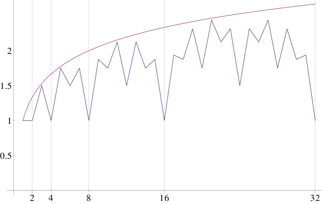
Figure 3: $D(N)=ND_{N}^{*}(Y_{2})$ of the van der Corput sequence in base 2 for $N=1,2,\ldots,32$, compared with $N\mapsto\tfrac{\log N}{3\log 2}+1$. Observe how the recursion (10) is reflected in the graph, for example, $D(1)=D(2)=D(4)=D(8)=D(16)=D(32)$.

Based on formula (9) Béjian and Faure reproved the discrepancy estimate (8). Furthermore they showed:

Theorem 2 (Béjian and Faure)

We have

$$\limsup_{N\rightarrow\infty}\left(ND_{N}^{\ast}(Y_{2})-\frac{\log N}{3\log 2}\right)=\frac{4}{9}+\frac{\log 3}{3\log 2}$$

and

$$\frac{1}{M}\sum_{N=1}^{M}ND_{N}^{\ast}(Y_{2})=\frac{\log M}{4\log 2}+O(1).$$

Using (9), Béjian and Faure also provided the intervals for which the discrepancy is attained:

Corollary 1

The reals $\alpha\in[0,1)$ for which $\Delta_{Y_{2},N}(\alpha)=D_{N}(Y_{2})$ are those for which there exists a sequence $(\varepsilon_{r})_{r\geq 1}$ of signs $\varepsilon_{r}\in\{+,-\}$ such that

$$\alpha=-\sum_{r=1}^{\infty}\frac{1}{2^{r}}\left\|\frac{N}{2^{r}}\right\|^{\prime}_{\varepsilon_{r}}\pmod{1}$$

where $\left\|\cdot\right\|^{\prime}_{+}$ and $\left\|\cdot\right\|^{\prime}_{-}$ are the right and the left derivatives of $\left\|\cdot\right\|$, respectively.

Note that the number of the intervals given in Corollary 1 is the greatest power of 2 dividing $N$.

A further result whose proof is based on (9) is the following central limit theorem for the star discrepancy of $Y_{2}$.

Theorem 3 (Drmota, Larcher, and Pillichshammer)

For every real $y$ and for $M\rightarrow\infty$ we have

$$\frac{1}{M}\#\left\{N<M:ND_{N}^{*}(Y_{2})\leq\frac{\log N}{4\log 2}+\frac{y}{4}\sqrt{\frac{\log N}{3\log 2}}\right\}=\Phi(y)+o(1),$$

where

$$\Phi(y)=\frac{1}{\sqrt{2\pi}}\int\limits_{-\infty}^{y}\exp(-t^{2}/2)\,\mathrm{d}t$$

denotes the Gaussian cumulative distribution function. That is, the star discrepancy of the van der Corput sequence in base $2$ satisfies a central limit theorem.

Proof sketch. It suffices to prove the equivalent limit relation

$$\frac{1}{M}\#\left\{N<M:ND_{N}^{*}(Y_{2})\leq\frac{\log M}{4\log 2}+\frac{y}{4}\sqrt{\frac{\log M}{3\log 2}}\right\}=\Phi(y)+o(1).$$ (11)

Assume first that $M=2^{m}$. Using formula (9) one can show that

$$ND_{N}^{*}(Y_{2})=\sum_{r=1}^{m}\|\omega 2^{r}\|+O(1),$$

where $\omega$ is uniformly distributed on $[0,1)$. Now, by using well known limit theorems for lacunary sequences (compare with [59] and [115], alternatively we can use [136]) it follows that

$$S_{m}=\sum_{r=1}^{m}\|\omega 2^{r}\|$$

satisfies a central limit theorem. Since ${\bf E}[S_{m}]=m/4$ and ${\bf Var}[S_{m}]=m/48$ we thus have

$$\frac{S_{m}-m/4}{\sqrt{m/48}}\to N(0,1),$$

and also all moments converge. Since $ND_{N}^{*}(Y_{2})=S_{m}+O(1)$ we get the same limit relation for $ND_{N}^{*}(Y_{2})$ if $N$ is uniformly distributed on $\{0,1,\ldots,2^{m}-1\}$. This proves the theorem for $M=2^{m}$. The general case, where $M$ is not a power of $2$, can be reconstructed from the case of $M=2^{m}$ by considering moments. A detailed version of this proof can be found in [27, Proof of Theorem 2]. $\hfill\Box\vspace{0.5cm}$

Remark 2

It is known from [7, Théorème 1] that $D_{N}^{*}(Y_{2})=D_{N}(Y_{2})$. Hence the presented results for the star discrepancy of $Y_{2}$ remain valid if we replace the star discrepancy by the extreme discrepancy.

Central limit theorems for the star discrepancy of van der Corput sequences in arbitrary bases $b$ can be found in the PhD thesis of Wohlfarter [145].

The $L_{p}$-discrepancy.

For the $L_{p}$-discrepancy of the van der Corput sequence in base $2$ the situation is a bit different than for the star discrepancy. The most studied case is the case $p=2$. Similar to (9) Faure [37] proved the following explicit formula:

$$4(NL_{2,N}(Y_{2}))^{2}=\left(\sum_{j=1}^{\infty}\left\|\frac{N}{2^{j}}\right\|\right)^{2}+\sum_{j=1}^{\infty}\left\|\frac{N}{2^{j}}\right\|^{2}.$$ (12)

Based on this formula he was able to show the following results for the $L_{2}$-discrepancy of the van der Corput sequence in base $2$:

Theorem 4 (Faure)

For all $N\in\mathbb{N}$ we have

$$(NL_{2,N}(Y_{2}))^{2}\leq\left(\frac{\log N}{6\log 2}\right)^{2}+\left(\frac{11}{3}+\frac{2\log 3}{\log 2}\right)\frac{\log N}{36\log 2}+\frac{1}{3}.$$

Moreover

$$\limsup_{N\rightarrow\infty}\left((NL_{2,N}(Y_{2}))^{2}-\left(\frac{\log N}{6\log 2}\right)^{2}-\left(\frac{11}{3}-\frac{2\log 3}{\log 2}\right)\frac{\log N}{36\log 2}\right)$$

$$=\frac{7}{81}+\frac{11\log 3}{108\log 2}+\left(\frac{\log 3}{6\log 2}\right)^{2}.$$

A proof of these results can be found in [37], where a similar study is also performed for the symmetrized version of the van der Corput sequence (see Section 3.1 for details).

For $p\geq 1$, the following estimates are known.

Theorem 5 (Pillichshammer)

Let $p\geq 1$. For all $N\in\mathbb{N}$ we have

$$(NL_{p,N}(Y_{2}))^{p}\leq\left(\frac{\log N}{6\log 2}\right)^{p}+O((\log N)^{p-1}),$$

where the constant in the $O$-notation only depends on $p$. If $N$ is of the form

$$N=\frac{2^{m+1}}{3}\left(1-\left(-\frac{1}{2}\right)^{m+1}\right)$$

we have

$$(NL_{p,N}(Y_{2}))^{p}\geq\frac{1}{2^{p}}\left(\frac{m}{3}+\frac{1}{9}-(-1)^{m}\frac{1}{9\cdot 2^{m}}\right)^{p}.$$

In particular,

$$\limsup_{N\rightarrow\infty}\frac{NL_{p,N}(Y_{2})}{\log N}=\frac{1}{6\log 2}=0.2404\ldots.$$ (13)

A proof of these results can be found in [117]. Equation (13) for $1\leq p\leq 2$ can also be found in [16, 121] and for $p=2$ in [63].

A comparison of Theorem 5 with (7) shows that the $L_{p}$-discrepancy of the van der Corput sequence in base 2 is not of optimal order of magnitude in $N$. This problem can be overcome with a symmetrization technique which will be explained in Section 3.1.

On average the $L_{p}$-discrepancy of the van der Corput sequence is large but behaves very regularly, as can be seen from the following theorem, which is [27, Theorem 3].

Theorem 6 (Drmota, Larcher, and Pillichshammer)

For every $p\geq 1$, for every real $y$, and for $M\rightarrow\infty$ we have

$$\frac{1}{M}\#\left\{N<M:NL_{p,N}(Y_{2})\leq\frac{\log N}{8\log 2}+\frac{y}{8}\sqrt{\frac{\log N}{3\log 2}}\right\}=\Phi(y)+o(1),$$

that is, the $L_{p}$-discrepancy satisfies a central limit theorem.

2.3 The discrepancy of the generalized van der Corput sequence

Definition of the generalized van der Corput sequence.

This type of sequence was introduced by Faure [32] with the aim of improving the constant term in the asymptotic behavior of low-discrepancy sequences.

Definition 2

Let $b\in\mathbb{N}$, $b\geq 2$, and let $\Sigma=(\sigma_{r})_{r\geq 0}$ be a sequence of permutations of $\{0,1,\ldots,b-1\}=:\mathbb{Z}_{b}$.

• The $b$-adic radical inverse function with respect to $\Sigma$ is defined as $Y_{b}^{\Sigma}:\mathbb{N}_{0}\rightarrow[0,1)$,

  $$Y_{b}^{\Sigma}(n)=\frac{\sigma_{0}(n_{0})}{b}+\frac{\sigma_{1}(n_{1})}{b^{2}}+\frac{\sigma_{2}(n_{2})}{b^{3}}+\cdots,$$

  for $n\in\mathbb{N}_{0}$ with $b$-adic digit expansion $n=n_{0}+n_{1}b+n_{2}b^{2}+\cdots$, where $n_{i}\in\mathbb{Z}_{b}$.

• The generalized van der Corput sequence in base $b$ associated with $\Sigma$ is defined as $Y_{b}^{\Sigma}:=(y_{n})_{n\geq 0}$ with $y_{n}=Y_{b}^{\Sigma}(n)$.

If $\Sigma=(\sigma)_{r\geq 0}$ is constant, we simply write $Y_{b}^{\Sigma}=Y_{b}^{\sigma}$. The original van der Corput sequence $Y_{b}$ in base $b$ is obtained with the identical permutation, i.e., $Y_{b}=Y_{b}^{{\rm id}}$.

It is an easy extension of the classical case of $Y_{b}$ that for every $\Sigma$ the generalized van der Corput sequence in base $b$ associated with $\Sigma$ is uniformly distributed modulo 1. See also [32, Propriété 3.1.1] for a short proof using a result on $b$-additive functions.

Functions related to a pair $(b,\sigma)$.

In [32] and [16] the formulas (9) and (12) were fully generalized. To recall these formulas we first need to introduce some definitions used in the study of generalized van der Corput sequences. For $J\subseteq[0,1)$ and $X=(x_{n})_{n\geq 0}$ let $A(J;N;X)$ be the number of indices $n\in\{0,1,\ldots,N-1\}$ such that $x_{n}\in J$.

Let $\mathfrak{S}_{b}$ be the set of all permutations of $\mathbb{Z}_{b}$. For any $\sigma\in\mathfrak{S}_{b}$ set

$$\mathcal{Z}_{b}^{\sigma}=\left(\tfrac{\sigma(0)}{b},\tfrac{\sigma(1)}{b},\ldots,\tfrac{\sigma(b-1)}{b}\right).$$

For $h\in\mathbb{Z}_{b}$ and $x\in[(k-1)/b,k/b)$, where $k\in\{1,\ldots,b\}$, define

$$\varphi_{b,h}^{\sigma}(x)=\left\{\begin{array}[]{ll}A([0,h/b);k;\mathcal{Z}_{b}^{\sigma})-hx&\mbox{ if }0\leq h\leq\sigma(k-1),\\ (b-h)x-A([h/b,1);k;\mathcal{Z}_{b}^{\sigma})&\mbox{ if }\sigma(k-1)<h<b.\end{array}\right.$$

Note that $\varphi_{b,0}^{\sigma}=0$ for any $\sigma\in\mathfrak{S}_{b}$. Further we observe that if $b=2$, then we only have two permutations which give either $\varphi_{2,1}^{\sigma}=\|\cdot\|$ if $\sigma$ is the identity or $\varphi_{2,1}^{\sigma}=-\|\cdot\|$ if $\sigma$ is the transposition $(0\,1)$.

Moreover, the functions $\varphi_{b,h}^{\sigma}$ are extended to the reals by periodicity. Based on $\varphi_{b,h}^{\sigma}$ we define further functions which then appear in the formulas for different notions of discrepancy. Put

$$\psi_{b}^{\sigma,+}=\max_{0\leq h<b}\varphi_{b,h}^{\sigma}\;,\;\;\;\psi_{b}^{\sigma,-}=\max_{0\leq h<b}(-\varphi_{b,h}^{\sigma}),\;\;\psi_{b}^{\sigma}=\psi_{b}^{\sigma,+}+\psi_{b}^{\sigma,-},$$

$$\varphi_{b}^{\sigma}=\sum_{h=0}^{b-1}\varphi_{b,h}^{\sigma}\ ,\;\;\phi_{b}^{\sigma}=\sum_{h=0}^{b-1}\left(\varphi_{b,h}^{\sigma}\right)^{2}\ \mbox{ and }\chi_{b}^{\sigma}=b\phi_{b}^{\sigma}-(\varphi_{b}^{\sigma})^{2}.$$

Note that $\psi_{b}^{\sigma}=\max_{0\leq h<h^{\prime}<b}|\varphi_{b,h}^{\sigma}-\varphi_{b,h^{\prime}}^{\sigma}|$  and  $\chi_{b}^{\sigma}=\sum_{0\leq h<h^{\prime}<b}(\varphi_{b,h}^{\sigma}-\varphi_{b,h^{\prime}}^{\sigma})^{2}$.

Exact formulas.

For a sequence $X=(x_{n})_{n\geq 0}$ in $[0,1)$ let

$$D_{N}^{+}(X)=\sup_{0\leq t\leq 1}\Delta_{X,N}(t)\ \ \ \mbox{ and }\ \ \ D_{N}^{-}(X)=\sup_{0\leq t\leq 1}(-\Delta_{X,N}(t)).$$

The following theorems link, with exact formulas, the functions defined above to the discrepancy of generalized van der Corput sequences. Note that the infinite series in these formulas can in fact be represented as the sum of finite terms and geometric series, and hence can be computed exactly (see [32, 3.3.6 Corollaire 1] for $D_{N},D_{N}^{+},D_{N}^{-}$; analogous proofs hold for $L_{2,N}$ and $F_{N}$). We first give the formulas for the extreme discrepancies obtained in [32, Théorème 1]:

Theorem 7 (Faure)

For any $N\in\mathbb{N}$ we have

$$ND^{+}_{N}(Y_{b}^{\Sigma})=\sum_{j=1}^{\infty}\psi_{b}^{\sigma_{j-1},+}\left(\frac{N}{b^{j}}\right),$$

$$ND^{-}_{N}(Y_{b}^{\Sigma})=\sum_{j=1}^{\infty}\psi_{b}^{\sigma_{j-1},-}\left(\frac{N}{b^{j}}\right),$$

$$ND_{N}(Y_{b}^{\Sigma})=\sum_{j=1}^{\infty}\psi_{b}^{\sigma_{j-1}}\left(\frac{N}{b^{j}}\right)\mbox{ and }$$

$$D_{N}^{\ast}(Y_{b}^{\Sigma})=\max(D^{+}_{N}(Y_{b}^{\Sigma}),D^{-}_{N}(Y_{b}^{\Sigma})).$$

Next, we state the formulas for $L_{2,N},F_{N}$, and $L_{1,N}$ obtained in [16, Théorèmes 4.1, 4.2, 4.3], but in a fixed base $b$ instead of in variable bases as in [16]:

Theorem 8 (Chaix and Faure)

For any $N\in\mathbb{N}$, we have

$$(NL_{2,N}(Y_{b}^{\Sigma}))^{2}=\\ \frac{1}{b}\sum_{j=1}^{\infty}\phi_{b}^{\sigma_{j-1}}\left(\frac{N}{b^{j}}\right)+\frac{1}{b^{2}}\sum_{i\neq j}\varphi_{b}^{\sigma_{i-1}}\left(\frac{N}{b^{i}}\right)\varphi_{b}^{\sigma_{j-1}}\left(\frac{N}{b^{j}}\right),$$

$$(NF_{N}(Y_{b}^{\Sigma}))^{2}=\frac{4\pi^{2}}{b^{2}}\sum_{j=1}^{\infty}\chi_{b}^{\sigma_{j-1}}\left(\frac{N}{b^{j}}\right)\ \ \ \mbox{ and }$$

$$NL_{1,N}(Y_{b})=\frac{1}{b}\sum_{j=1}^{\infty}\varphi_{b}^{{\rm id}}\left(\frac{N}{b^{j}}\right).$$

Asymptotic behavior for the extreme and star discrepancies.

Concerning the asymptotic behavior of the extreme discrepancy $D_{N}$, the following generalization of (8) to arbitrary bases with fixed permutations was proved in [32, Théorème 2]:

Theorem 9 (Faure)

For $\sigma\in\mathfrak{S}_{b}$ and for all $N\in\mathbb{N}$ we have

$$D_{N}(Y_{b}^{\sigma})\leq\frac{1}{N}\left(\frac{\alpha_{b,\sigma}}{\log b}\log N+\max\left(2,1+\frac{1}{b}+\alpha_{b,\sigma}\right)\right),$$

where

$$\alpha_{b,\sigma}=\inf_{m\geq 1}\sup_{x\in\mathbb{R}}\left(\frac{1}{m}\sum_{j=1}^{m}\psi_{b}^{\sigma}\left(\frac{x}{b^{j}}\right)\right).$$

Moreover,

$$d(Y_{b}^{\sigma}):=\limsup_{N\rightarrow\infty}\frac{ND_{N}(Y_{b}^{\sigma})}{\log N}=\frac{\alpha_{b,\sigma}}{\log b}.$$ (14)

Remark 3

In particular, see [32, Théorème 6], for $\sigma={\rm id}$ we have (the best constant being obtained for $b=3$ with $\alpha_{3,{\rm id}}=1/2\log 3$)

$$\alpha_{b,{\rm id}}=\left\{\begin{array}[]{ll}\displaystyle\frac{b^{2}}{4(b+1)}&\mbox{ if $b$ is even,}\\ \displaystyle\frac{b-1}{4}&\mbox{ if $b$ is odd.}\end{array}\right.$$ (15)

It is worth noting that $\psi_{b}^{{\rm id},-}=0$, so that $\psi_{b}^{{\rm id}}=\psi_{b}^{{\rm id},+}$ and hence $D_{N}(Y_{b})=D_{N}^{*}(Y_{b})$ for the van der Corput sequence $Y_{b}$. Equation (15) shows that $D_{N}(Y_{b})$ increases and tends to infinity with $b$. The question of the existence of a permutation $\sigma_{b}$ such that $d(Y_{b}^{\sigma_{b}})$ is bounded (by an absolute constant) can be answered positively, see Section 3.3.

Theorem 9 is the starting point for research on best possible upper bounds for the extreme discrepancy $D_{N}$, see the end of the present Section 2.3. In the next theorem, we give an analogous result for the star discrepancy $D_{N}^{*}$ in a slightly different form than the original version in [32, Théorème 3]:

Theorem 10 (Faure)

Let $\tau_{b}\in\mathfrak{S}_{b}$ be the permutation defined by $\tau_{b}(k)=b-k-1$ for all $k\in\mathbb{Z}_{b}$ and let $\mathcal{A}$ be the subset of $\mathbb{N}_{0}$ defined by $\mathcal{A}=\bigcup_{H=1}^{\infty}\mathcal{A}_{H}$ with $\mathcal{A}_{H}=\{H(H-1),\ldots,H^{2}-1\}$. For any permutation $\sigma\in\mathfrak{S}_{b}$, let $\overline{\sigma}:=\tau_{b}\circ\sigma$ and let

$$\Sigma^{\sigma}_{\mathcal{A}}=(\sigma_{r})_{r\geq 0}:=(\sigma,\overline{\sigma},\sigma,\sigma,\overline{\sigma},\overline{\sigma},\sigma,\sigma,\sigma,\overline{\sigma},\overline{\sigma},\overline{\sigma},\ldots)$$

be the sequence of permutations defined by $\sigma_{r}=\sigma$ if $r\in\mathcal{A}$ and $\sigma_{r}=\overline{\sigma}$ if $r\notin\mathcal{A}$. Then

$$d^{*}(Y_{b}^{\Sigma^{\sigma}_{\mathcal{A}}}):=\limsup_{N\rightarrow\infty}\frac{ND_{N}^{*}(Y_{b}^{\Sigma^{\sigma}_{\mathcal{A}}})}{\log N}=\frac{\alpha_{b,\sigma}^{+}+\alpha_{b,\sigma}^{-}}{2\log b},$$ (16)

where

$$\alpha_{b,\sigma}^{+}=\inf_{m\geq 1}\frac{1}{m}\sup_{x\in[0,1]}\sum_{j=1}^{m}\psi_{b}^{\sigma,+}\left(\frac{x}{b^{j}}\right)\quad\mbox{ and }\quad\alpha_{b,\sigma}^{-}=\inf_{m\geq 1}\frac{1}{m}\sup_{x\in[0,1]}\sum_{j=1}^{m}\psi_{b}^{\sigma,-}\left(\frac{x}{b^{j}}\right).$$

Remark 4 (On the “swapping” permutation $\tau_{b}$)

Let $\mathcal{S}$ be a subset of $\mathbb{N}_{0}$ and let $\sigma\in\mathfrak{S}_{b}$. Define the sequence ${\Sigma^{\sigma}_{\mathcal{S}}}=(\sigma_{r})_{r\geq 0}$ by $\sigma_{r}=\sigma$ if $r\in\mathcal{S}$ and $\sigma_{r}=\overline{\sigma}=\tau_{b}\circ\sigma$ if $r\notin\mathcal{S}$. Then, see [32, Lemme 4.4.1], we have

$$ND^{+}_{N}(Y_{b}^{\Sigma^{\sigma}_{\mathcal{S}}}) = \sum_{j=1\atop j\in\mathcal{S}}^{\infty}\psi_{b}^{\sigma,+}\left(\frac{N}{b^{j}}\right)+\sum_{j=1\atop j\notin\mathcal{S}}^{\infty}\psi_{b}^{\sigma,-}\left(\frac{N}{b^{j}}\right)\ \mbox{ and }$$

$$ND^{-}_{N}(Y_{b}^{{\Sigma^{\sigma}_{\mathcal{S}}}}) = \sum_{j=1\atop j\in\mathcal{S}}^{\infty}\psi_{b}^{\sigma,-}\left(\frac{N}{b^{j}}\right)+\sum_{j=1\atop j\notin\mathcal{S}}^{\infty}\psi_{b}^{\sigma,+}\left(\frac{N}{b^{j}}\right).$$

The permutation $\tau_{b}$ swaps the functions $\psi_{b}^{\sigma,+}$ and $\psi_{b}^{\sigma,-}$ and hence, in order to minimize $D_{N}^{*}=\max(D_{N}^{+},D_{N}^{-})$, one has to find a set $\mathcal{S}$ for which the sums with $\psi_{b}^{\sigma,+}$ and $\psi_{b}^{\sigma,-}$ asymptotically split into two equal parts. This is achieved, for example, by the set $\mathcal{A}=\{0,2,3,6,7,8,12,13,14,15,\ldots\}$ introduced in Theorem 10 above. Further, since $\psi_{b}^{\sigma,+}+\psi_{b}^{\sigma,-}=\psi_{b}^{\sigma}$, for any $\mathcal{S}\subseteq\mathbb{N}_{0}$, we have

$$D_{N}(Y_{b}^{\Sigma^{\sigma}_{\mathcal{S}}})=D^{+}_{N}(Y_{b}^{\Sigma^{\sigma}_{\mathcal{S}}})+D^{-}_{N}(Y_{b}^{{\Sigma^{\sigma}_{\mathcal{S}}}})=\sum_{j=1}^{\infty}\left(\psi_{b}^{\sigma,+}\left(\frac{N}{b^{j}}\right)+\psi_{b}^{\sigma,-}\left(\frac{N}{b^{j}}\right)\right)=D_{N}(Y_{b}^{\sigma}).$$

This property is the starting point for research on best possible lower bounds for the star discrepancy for the family of $Y_{b}^{\Sigma}$ sequences, and for a new generalization of this family, see Section 3.2.

Remark 5

For reasonably small $b$, the constants $\alpha_{b,\sigma}^{+}$ and $\alpha_{b,\sigma}^{-}$ are not difficult to compute, and for the identical permutation (for which $\psi_{b}^{{\rm id},-}=0$) it is even possible to find them explicitly: from (15), for arbitrary $b$ we obtain

$$d^{*}(Y_{b}^{\Sigma^{\rm id}_{\mathcal{A}}})=\frac{\alpha_{b,{\rm id}}^{+}}{2\log b}=\left\{\begin{array}[]{ll}\displaystyle\frac{b^{2}}{8(b+1)\log b}&\mbox{ if }b\mbox{ is even,}\\ \displaystyle\frac{b-1}{8\log b}&\mbox{ if }b\mbox{ is odd.}\end{array}\right.$$ (17)

For $b=2$, this result was first obtained by Béjian [5] and then rediscovered in [80] in the context of shifted Hammersley and van der Corput point sets. The result in [80] states that

$$ND_{N}^{\ast}(Y_{2}^{\Sigma^{\rm id}_{\mathcal{A}}})\leq\frac{\log N}{6\log 2}+c\sqrt{\log N},$$ (18)

for all $N\in\mathbb{N}$, where $c>0$ is a constant and where the constant $1/(6\log 2)$ is best possible. We thus see that there exists an explicit generalized version of $Y_{2}$ which reduces the constant in (8) by a factor of 2, and this reduction is best possible.

It is also worth mentioning the following result from [80] for general sequences $\Sigma$ and $b=2$ which reflects the properties of $\Sigma$ in order to obtain a low star discrepancy. For $m\in\mathbb{N}$ let

$$S_{m}(\Sigma):=\max\left(\#\{0\leq r\leq m-1:\ \sigma_{r}=\tau_{2}\},\#\{0\leq r\leq m-1:\ \sigma_{r}=\mathrm{id}\}\right)$$

and

$$T_{m}(\Sigma):=\#\{1\leq r\leq m-1:\ \sigma_{r-1}=\tau_{2}\ \mbox{and}\ \sigma_{r}={\rm id}\}.$$

The quantities $S_{m}(\Sigma)$ and $T_{m}(\Sigma)$ can be used to give very precise discrepancy estimates for a generalized van der Corput sequence based on $\Sigma$. The following theorem was shown in [80].

Theorem 11 (Kritzer, Larcher, and Pillichshammer)

Let $\Sigma=(\sigma_{r})_{r\geq 0}$ be a sequence of permutations of $\mathbb{Z}_{2}$, and let $Y_{2}^{\Sigma}$ be the corresponding generalized van der Corput sequence. Then it is true that

$$\frac{S_{m}(\Sigma)}{3}+\frac{T_{m}(\Sigma)}{48}-4\leq\max_{1\leq N\leq 2^{m}}ND_{N}^{\ast}(Y_{2}^{\Sigma})\leq\frac{S_{m}(\Sigma)}{3}+\frac{2T_{m}(\Sigma)}{9}+\frac{56}{9}.$$

Theorem 11 implies that two properties of $\Sigma$ influence the star discrepancy of the shifted van der Corput sequence. On the one hand, it is the number of identical permutations ${\rm id}$ compared to the number of transpositions $\tau_{2}$ in $\Sigma$, and on the other hand, it is also how these are distributed. Obviously, it is favorable to have a situation where, for as many $m\in\mathbb{N}$ as possible, approximately half of the permutations among the first $m$ elements of $\Sigma$ is the identity, and simultaneously there should not be too many changes between ${\rm id}$ and $\tau_{2}$. This observation is perfectly reflected in the star discrepancy estimate for $Y_{2}^{\Sigma^{\rm id}_{\mathcal{A}}}$ presented above in (18).

Asymptotic behavior of the $L_{2}$-discrepancy and the diaphony.

As for Theorem 9, Theorem 10 is the starting point for research on best possible upper bounds for the star discrepancy (see the end of Section 2.3). These theorems have analogous formulations, resulting from Theorem 8, for the $L_{p}$-discrepancy and for the diaphony $F_{N}$. We only give an excerpt of a series of results in fixed and variable bases that can be found in [16, Section 4.2]:

Theorem 12 (Chaix and Faure)

For $\sigma\in\mathfrak{S}_{b}$ and for all $N\in\mathbb{N}$ we have

$$t_{1}(Y_{b}^{\sigma}):=\limsup_{N\rightarrow\infty}\frac{NL_{2,N}(Y_{b}^{\sigma})}{\log N}=\frac{\beta_{b,\sigma}}{b\log b}\ \mbox{ with }\ \beta_{b,\sigma}=\inf_{m\geq 1}\sup_{x\in\mathbb{R}}\left(\frac{1}{m}\sum_{j=1}^{m}\varphi_{b}^{\sigma}\left(\frac{x}{b^{j}}\right)\right),$$

and

$$f(Y_{b}^{\sigma}):=\limsup_{N\rightarrow\infty}\frac{(NF_{N}(Y_{b}^{\sigma}))^{2}}{\log N}=\frac{4\pi^{2}\gamma_{b,\sigma}}{b^{2}\log b}\ \mbox{ with }\ \gamma_{b,\sigma}=\inf_{m\geq 1}\sup_{x\in\mathbb{R}}\left(\frac{1}{m}\sum_{j=1}^{m}\chi_{b}^{\sigma}\left(\frac{x}{b^{j}}\right)\right).$$

Theorem 12 confirms that the generalized van der Corput sequences $Y_{b}^{\sigma}$ do not have optimal $L_{2}$-discrepancy with respect to the order of magnitude in $N$, which would be $O(\sqrt{\log N}/N)$.

Remark 6

In particular, see [16, Théorèmes 4.12 and 4.13], for $\sigma={\rm id}$ we have:

$$t_{1}(Y_{b}^{\rm id})=\left\{\begin{array}[]{ll}\displaystyle\frac{b^{2}+b-2}{8(b+1)\log b}&\mbox{ if $b$ is even,}\\ \displaystyle\frac{b^{2}-1}{8b\log b}&\mbox{ if $b$ is odd,}\end{array}\right.$$

(cf. Theorem 4 for $b=2$) and

$$f(Y_{b}^{\rm id})=\left\{\begin{array}[]{ll}\displaystyle\frac{\pi^{2}(b^{3}+b^{2}+4)}{48(b+1)\log b}&\mbox{ if $b$ is even,}\\ \displaystyle\frac{\pi^{2}(b^{4}+2b^{2}-3)}{48b^{2}\log b}&\mbox{ if $b$ is odd.}\end{array}\right.$$

These exact values for $f(Y_{b}^{\rm id})$ are about four times smaller than the upper bound obtained by Pagès with the von Neumann-Kakutani transformation, see [113, Proposition 2.5].

We now summarize the results from [82], where the $L_{2}$-discrepancy of $Y_{2}^{\Sigma}$ is considered. From Theorem 4, we know that

$$NL_{2,N}(Y_{2})\sim\frac{\log N}{6\log 2}.$$ (19)

Again, the question arises how the $L_{2}$-discrepancy of $Y_{2}^{\Sigma}$ is influenced by the properties of $\Sigma$. Opposed to the star discrepancy, here one may ask not only whether the constant in the $\log N$-term can be improved, but, in view of (7), also whether one could possibly obtain a better order of magnitude. To give precise answers, we proceed in a way that resembles the results for the star discrepancy. Let $\Sigma=(\sigma_{r})_{r\geq 0}$ be a sequence of permutations of $\mathbb{Z}_{2}$, and define, for $m\in\mathbb{N}$,

$$Z_{m}(\Sigma):=\#\{0\leq r\leq m-1:\ \sigma_{r}=\mathrm{id}\}.$$

Furthermore, let $z_{m}(\Sigma):=Z_{m}(\Sigma)-\frac{m}{2}$. Using the quantity $z_{m}$ the following average-type result was shown in [82].

Theorem 13 (Kritzer and Pillichshammer)

Let $\Sigma=(\sigma_{r})_{r\geq 0}$ be a sequence of permutations of $\mathbb{Z}_{2}$ for which $A:=\lim_{m\rightarrow\infty}\frac{(z_{m}(\Sigma))^{2}}{m}$ exists. Then the following two statements are true:

• $$\limsup_{m\rightarrow\infty}\frac{1}{2^{m}}\sum_{N=1}^{2^{m}}\frac{(NL_{2,N}(Y_{2}^{\Sigma}))^{2}}{m}<\frac{A}{16}+\frac{4}{3}.$$

• For any $\varepsilon>0$ we have

  $$\lim_{m\rightarrow\infty}\frac{\#\{1\leq N\leq 2^{m}:\ NL_{2,N}(Y_{2}^{\Sigma})<(\log N)^{1/2+\varepsilon}\}}{2^{m}}=1.$$

Considering the result in Theorem 13, one might hope that there is a sequence $\Sigma$ such that the order of magnitude in $N$ of $L_{2,N}(Y_{2}^{\Sigma})$ is lower than that of $L_{2,N}(Y_{2})$. Unfortunately, these hopes are crushed by the following result that was also shown in [82].

Theorem 14 (Kritzer and Pillichshammer)

There exists a positive constant $c$ such that for all sequences $\Sigma=(\sigma_{r})_{r\geq 0}$ of permutations of $\mathbb{Z}_{2}$ we have

$$NL_{2,N}(Y_{2}^{\Sigma})\geq c\log N\ \ \ \mbox{for infinitely many $N\in\mathbb{N}$.}$$

As we see from this theorem, we cannot improve the order of the $L_{2}$-discrepancy of $Y_{2}$ by permutations, but we can again ask whether one can at least improve the constants in (19). For this question, there is a positive answer which implies that permutations never worsen the constant in (19) and can even improve the constant considerably. The following result is also due to [82].

Theorem 15 (Kritzer and Pillichshammer)

It is true that

$$\sup_{\Sigma}\limsup_{N\rightarrow\infty}\frac{NL_{2,N}(Y_{2}^{\Sigma})}{\log N}=\frac{1}{6\log 2},$$

$$\inf_{\Sigma}\limsup_{N\rightarrow\infty}\frac{NL_{2,N}(Y_{2}^{\Sigma})}{\log N}\leq\frac{1}{20\log 2},$$

where the supremum and the infimum, respectively, are extended over all sequences $\Sigma$ of permutations of $\mathbb{Z}_{2}$.

Regarding the latter result, one can show that the value $\tfrac{1}{20\log 2}$ is attained for the sequence $\Sigma$ in which the identical permutation $\mathrm{id}$ and the transposition $\tau_{2}$ alternate. It is even conjectured that this result is best possible with respect to all choices of $\Sigma$. Note that, if the conjecture is correct, this would mark a difference to the star discrepancy, where an alternating sequence $\Sigma$ has disadvantages due to the role of the quantity $T_{m}(\Sigma)$ in Theorem 11. For the $L_{2}$-discrepancy it seems to be the case that, while $S_{m}$ also plays a crucial role, the value of $T_{m}$ has no influence on the results.

The state of the art for asymptotic constants related to $D_{N},D_{N}^{*},L_{2,N}$, and $F_{N}$.

Generalizations of van der Corput sequences give the smallest discrepancies and diaphony currently known within the class of infinite one-dimensional sequences $X$ in $[0,1)$. We need the following quality parameters to present these current “records”. Let

$$d:=\inf_{X}(d(X))=\inf_{X}\left(\limsup_{N\rightarrow\infty}\frac{ND_{N}(X)}{\log N}\right),\ \ \ d^{*}:=\inf_{X}(d^{*}(X))=\inf_{X}\left(\limsup_{N\rightarrow\infty}\frac{ND^{*}_{N}(X)}{\log N}\right),$$

$$t_{1}:=\inf_{X}(t_{1}(X))=\inf_{X}\left(\limsup_{N\rightarrow\infty}\frac{NL_{2,N}(X)}{\log N}\right),\ \ \ t_{2}(X):=\limsup_{N\rightarrow\infty}\frac{(NL_{2,N}(X))^{2}}{\log N},$$

$$t_{2}:=\inf_{X}(t_{2}(X))\ \ \mbox{ and }\ \ f:=\inf_{X}(f(X))=\inf_{X}\left(\limsup_{N\rightarrow\infty}\frac{(NF_{N}(X))^{2}}{\log N}\right),$$

where the infima are taken over all infinite one-dimensional sequences $X$ in $[0,1)$.

For the extreme discrepancy $D_{N}$, it was shown, in chronological order, that $d<0.38$, in base 12 by Faure [32, Théorème 4] in 1981, $d<0.367$, in base 36 by Faure [38, Théorème 1.2] in 1992, and $d<0.354$ in base 84 by Ostromoukhov [112, Theorem 4] in 2009, in each case for a specific permutation of digits in the specified base. Hence with the lower bound from Béjian [6] in 1982, one has the current estimate

$$0.12<d<0.354.$$

For the star discrepancy $D_{N}^{*}$, it was shown, in chronological order, that $d^{*}<0.2236$, in base 12 by Faure [32, Théorème 4] in 1981, and $d^{*}<0.2223$ in base 60 by Ostromoukhov [112, Theorem 5] in 2009, in each case for a specific permutation of digits in the specified base. Hence with the lower bound from Larcher [88] in 2014 one has the current estimate

$$0.0646<d^{*}<0.2223.$$

Concerning the $L_{2}$-discrepancy, the best permutations for the set of $Y_{b}^{\sigma}$ sequences, denoted by $\sigma_{b}$, satisfy $\lim_{b\rightarrow\infty}t_{1}(Y_{b}^{\sigma_{b}})=0$, see [16, Théorème 4.14 and its proof]. However, this result is not surprising since $t_{1}=0$ as can be seen from the study of symmetrized sequences (see Section 3.1) where estimates for $t_{2}$ will be given.

Finally, for the diaphony, besides earlier results by Proinov and Grozdanov [123] with weak constants (around 15), it was shown, in chronological order, that $f<1.59$, in base 2 by Proinov and Atanassov [121] in 1988, $f<1.316$, in base 19 by Chaix and Faure [16, Théorème 4.16] in 1993 and $f<1.137$, in base 57 by Pausinger and Schmid [114, Theorem 3.2] in 2010. As to the lower bound, the only result we know is that of Proinov [119] from the year 1986 which states that $f>0.0002$.

Comparison with $(n\alpha)$-sequences.

Concerning the extreme discrepancy of $(n\alpha)$-sequences, Ramshaw [124] obtained

$$d((n\widetilde{\alpha}))=\frac{1}{5\log((\sqrt{5}+1)/2)}=0.4156\ldots$$

with the golden ration $\widetilde{\alpha}=\tfrac{\sqrt{5}+1}{2}$ and it is a widely held belief that $\inf_{\alpha}d((n\alpha))=d((n\widetilde{\alpha}))$. Concerning the star discrepancy of $(n\alpha)$-sequences, Dupain and Sós [29] proved that

$$\inf_{\alpha}d^{*}((n\alpha))=d^{*}((n\sqrt{2}))=\frac{1}{4\log(\sqrt{2}+1)}=0.2836\ldots.$$

2.4 The elementary descent method

Context, statement and comments.

In this section, we are going to give an illustration—on the simple example of the triadic van der Corput sequence $Y_{3}$—of the method yielding the results given in Sections 2.3, 2.6, 3.1, and 3.3 for the generalized van der Corput sequences $Y_{b}^{\Sigma}$. A more involved variant of this method also applies to NUT digital $(0,1)$-sequences in prime base and to a larger family, the so-called NUT $(0,1)$-sequences over $\mathbb{Z}_{b}$, that will be considered in Section 3.2. Before this illustration, it is necessary to state the fundamental lemma resulting from the descent method and leading to the results. However, we first need some notation and a discretization lemma to prepare this statement.

For convenience, in the following we define the error (the deviation from uniform distribution) as

$$E(x,N,X):=N\Delta_{X,N}(x)\mbox{ and then }E([x,y),N,X):=E(y,N,X)-E(x,N,X),$$

where $\Delta_{X,N}(x)$ is the local discrepancy defined in Section 2. Further, we call a rational number in $[0,1)$ an $m$-bit number if it belongs to the set $\mathbb{Q}(b^{m})=\{0,\tfrac{1}{b^{m}},\tfrac{2}{b^{m}},\ldots,\tfrac{b^{m}-1}{b^{m}}\}$.

Lemma 1 (discretization lemma)

Let $\alpha\in[0,1]$ and let $m,N$ be integers with $1\leq N\leq b^{m}$. Furthermore, let $u,v$ be $m$-bit numbers such that $u\leq\alpha<v$ and $v=u+b^{-m}$, and let $x$ be the unique element in $\{Y_{b}^{\Sigma}(0),\ldots,Y_{b}^{\Sigma}(b^{m}-1)\}$ such that $u\leq x<v$. Then, with $y(\alpha):=u$ if $\alpha\leq x$ and $y(\alpha):=v$ if $\alpha>x$, we have

$$E(\alpha,N,Y_{b}^{\Sigma})=E(y(\alpha),N,Y_{b}^{\Sigma})+(y(\alpha)-\alpha)N.$$

This is a classical discretization property resulting from the definition of $y(\alpha)$ which implies the equality of counting functions $A(\alpha;N;Y_{b}^{\Sigma})=A(y(\alpha);N;Y_{b}^{\Sigma})$. From Lemma 1 it follows that it suffices to know the values of the error $E(\alpha,N,Y_{b}^{\Sigma})$ for $\alpha\in\mathbb{Q}(b^{m})$. Exactly these values are given by the following lemma which is the key property in the proof of Theorem 7.

Lemma 2 (fundamental descent lemma)

Let $m,N$, and $\lambda$ be integers with $1\leq N\leq b^{m}$ and $1\leq\lambda<b^{m}$, and let $\lambda=\lambda_{1}b^{m-1}+\cdots+\lambda_{m-1}b+\lambda_{m}$ be the b-adic expansion of $\lambda$. Then

$$E\left(\frac{\lambda}{b^{m}},N,Y_{b}^{\Sigma}\right)=\sum_{j=1}^{m}\varphi_{b,\varepsilon_{j}}^{\sigma_{j-1}}\left(\frac{N}{b^{j}}\right),$$ (20)

where the functions $\varepsilon_{j}=\varepsilon_{j}(\lambda,m,N)$ are defined inductively by $\varepsilon_{m}=\eta_{m}=\lambda_{m}$ and, for $1\leq j<m$,

$$\eta_{j}=\lambda_{j}+\frac{\eta_{j+1}}{b}+\frac{1}{b}\left(\varphi_{b,\varepsilon_{j+1}}^{\sigma_{j}}\right)^{\prime}\left(\frac{N}{b^{j+1}}\right)\ \ \mbox{ where $g^{\prime}$ means the right derivative of $g$,}$$

$$\varepsilon_{j}=\eta_{j}\quad{\rm if}\quad 0\leq\eta_{j}<b,\quad{\rm and}\quad\varepsilon_{j}=0\quad{\rm if}\quad\eta_{j}=b.$$

The proof is a descending recursion for the $b$-adic resolution of the argument $y=\lambda/b^{m}$ from $m$ to 1. At each step, the $b$-adic resolution of $y$ is decreased by 1. The differences between the discrepancy functions in a reduction step is controlled by means of the functions $\varphi_{b,h}^{\sigma}$ while the relation between the intervals depends on the right derivatives of these functions.

With Lemmas 1 and 2, it is easy to obtain Theorem 7. For instance, consider $D_{N}^{+}$: First, from Lemma 1, we get

$$\lim_{m\rightarrow\infty}\ \sup_{y\in\mathbb{Q}(b^{m})}E(y,N,Y_{b}^{\Sigma})=D_{N}^{+}(Y_{b}^{\Sigma}).$$

Then, since $\psi_{b}^{\sigma,+}=\max_{0\leq h<b}\varphi_{b,h}^{\sigma}$, for any $m$-bit number $y\in\mathbb{Q}(b^{m})$ we get from Lemma 2 the upper bound

$$E(y,N,Y_{b}^{\Sigma})\leq\sum_{j=1}^{m}\psi_{b}^{\sigma_{j-1},+}\left(\frac{N}{b^{j}}\right).$$

Now, using the algorithm for the construction of the $\varepsilon_{j}$’s from the $\lambda_{j}$’s (at the end of Lemma 2) in reversed direction, it is easy to construct a $\widetilde{\lambda}\in\{0,1,\ldots,b^{m}-1\}$ for which the above upper bound is achieved by $E(\widetilde{\lambda}b^{-m},N,Y_{b}^{\Sigma})$. Finally, letting $m$ tend to $\infty$ gives the formula for $D_{N}^{+}$.

Theorem 8 is not so easy and needs a further lemma ([16, Lemme 5.3]) to explicitly compute the functions $\varepsilon_{j}$; this means that recovering the functions $\varphi_{b}^{\sigma}$ and $\phi_{b}^{\sigma}$ is more involved in this case.

There are four versions of Lemma 2: The first one was worked out for the study of the $L_{2}$-discrepancy of the original van der Corput sequence in base 2 and its symmetrized version [37, Lemme 2.2]. The second one is the generalization of the preceding one to arbitrary variable bases with arbitrary sequences of permutations (the so-called $Y_{B}^{\Sigma}$ sequences) in [16, Lemme 5.2] for the study of both the $L_{p}$-discrepancy and the diaphony. The third and fourth ones were necessary to extend the method to digital $(0,1)$-sequences [39, Lemma 6.2] and a generalization of these sequences that also includes $Y_{b}^{\Sigma}$ sequences [55, Lemma 2]. In Theorems 2 and 7 the descent method is only present in filigree since, at that time, the relation between the intervals at each step of the descent was not found yet, and it was not necessary to get formulas for the extreme discrepancies. For non-French speaking readers who would like to go thoroughly into the details of the descent method we recommend [39, Lemma 6.2] where $X_{b}^{C}$ has to be replaced by $Y_{b}^{\Sigma}$ and the formula there by Equation (20).

Illustration of the descent method.

The first $b^{m}$ points of $Y_{b}^{\Sigma}$, $y_{0},\ldots,y_{b^{m}-1}$, can be represented on a checkerboard $B_{m}$ of $b^{2m}$ squares as black squares according to their position $b^{m}y_{k}$ on the abscissa (where $[0,1)$ is identified with $[0,b^{m})$) and their index $k$ on the ordinate for $1\leq k\leq b^{m}$. This is possible because Equation (20) deals with $m$-bit numbers $\lambda/b^{m}$, the error $E(\lambda/b^{m},N,Y_{b}^{\Sigma})$ involves the $m$-bit part of $y_{k}=Y_{b}^{\Sigma}(k)$ only. Then, in this framework, the error is $b^{m}$ times the number $A$ of black squares minus the area of $[0,\lambda]\times[0,N]$ divided by $b^{m}$, i.e.,

$$\widetilde{E}(\lambda,N,B_{m}):=b^{m}E(\lambda/b^{m},N,Y_{b}^{\Sigma})=b^{m}A-\lambda N.$$

One step of the descent method can be described, and the idea of $\varphi$-functions pointed out, by means of this representation as explained in the following special case of $Y_{3}$, for the first step (from $m$ to $m-1$) and with $m=3$, i.e., $b^{m}=3^{3}=27$, see Figure 4.

Figure 4: Checkerboard $B_{3}$ corresponding to the first $3^{3}$ elements of $Y_{3}$.

We distinguish three cases corresponding to $9(i-1)<N\leq 9i$, where $i\in\{1,2,3\}$, and for each of them we distinguish the abscissas $\lambda$ of the form $3\mu$ (blue lines), $3\mu+1$ (red lines), and $3\mu+2$ (green lines). Concerning the three cases for $N$, the idea is to express the error by moving the abscissa $\lambda$ to the nearest multiple of 3, $3\mu$ or $3(\mu+1)$, say $3\nu$, in such a way that the black squares $(27y_{k},k)$ with $9(i-1)<k\leq 9i$ still remain in the new rectangle $[0,3\nu]\times[0,N]$ in the three cases. In this way, the process is the same for any $N$ within a given case, and it will give a single formula for the error. Further, $\widetilde{E}(3\nu,N,B_{3})=\widetilde{E}(3\nu,N-9(i-1),B_{3})$ since $\widetilde{E}(3\nu,9(i-1),B_{3})=0$, and hence (cf. Figure 5)

$$\widetilde{E}(3\nu,N,B_{3})=\widetilde{E}(\nu,N-9(i-1),B_{2}).$$

Figure 5: Checkerboard $B_{2}$ corresponding to the first $3^{2}$ elements of $Y_{3}$.

Figure 6: Graph of $\varphi_{3,0}^{\rm id}$ (blue), $\varphi_{3,1}^{\rm id}$ (red) and $\varphi_{3,2}^{\rm id}$ (green); $\psi_{3}^{{\rm id}}=\max(\varphi_{3,1}^{\rm id},\varphi_{3,1}^{\rm id})$.

Now, it remains to compute the difference $\delta=\widetilde{E}(\lambda,N,B_{3})-\widetilde{E}(3\nu,N,B_{3})$ for each of the nine possibilities to make the step from $B_{3}$ to $B_{2}$:

• If $\lambda=3\mu$ (blue lines) then for any $N$ we have $\delta=0$ and $\nu=\mu$.
  

• If $\lambda=3\mu+1$ (red lines) then for $0<N\leq 9$ we have $\delta=2N$ and $\nu=\mu+1$, and for $9<N\leq 27$ we have $\delta=27-N$ and $\nu=\mu$.
  

• If $\lambda=3\mu+2$ (green lines) then for $0<N\leq 18$ we have $\delta=N$ and $\nu=\mu+1$, and for $18<N\leq 27$ we have $\delta=2(27-N)$ and $\nu=\mu$.

Coming back to the remainder and setting $\varphi_{3,0}^{\rm id}=0$, $\varphi_{3,1}^{\rm id}(x)=\min(2x,1-x)$, and $\varphi_{3,2}^{\rm id}(x)=\min(x,2(1-x))$ (see Figure 6) it is easy to check that the three cases above lead to the first step of Equation (20), where $1<i\leq 3$ and $\varepsilon=\lambda\bmod 3$:

$$E\left(\frac{\lambda}{27},N,Y_{b}^{\Sigma}\right)=E\left(\frac{\nu}{9},N-9(i-1),Y_{b}^{\Sigma}\right)+\varphi_{3,\varepsilon}^{\rm id}\left(\frac{N}{27}\right).$$

The next steps follow in the same way, but it is necessary to control the intervals that appear inductively in the descending recursion which explains the sophisticated definition of the $\varepsilon_{j}$’s in Equation (20) and the length of the proof of this formula (5 pages in [39]).

Concluding this illustration for base 3, we give the analog of Theorem 2 for the triadic van der Corput sequence $Y_{3}$ and the corresponding graph (Figure 7) showing the structure of the discrepancy by means of the function $\psi_{3}^{\rm id}$, see [30].

Theorem 16 (Faure)

For $N\in\mathbb{N}$ we have

$$ND_{N}^{*}(Y_{3})=ND_{N}(Y_{3})=\sum_{r=1}^{\infty}\psi_{3}^{\rm id}\left(\frac{N}{3^{r}}\right)=\sum_{r=1}^{m}\psi_{3}^{\rm id}\left(\frac{N}{3^{r}}\right)+\frac{N}{3^{m}}\ \ \mbox{ whenever $1\leq N\leq 3^{m}$},$$ (21)

$$ND_{N}^{*}(Y_{3})\leq\frac{\log N}{2\log 3}+\frac{3}{4}+\frac{\log 2}{2\log 3},$$

and

$$\limsup_{N\rightarrow\infty}\left(ND_{N}^{*}(Y_{3})-\frac{\log N}{2\log 3}\right)=\frac{3}{4}+\frac{\log 2}{2\log 3}.$$

It is even possible to obtain generating formulas like for $Y_{2}$ (cf. (10)), but, due to the form of the function $\psi_{3}^{\rm id}$, they are not as simple as for $Y_{2}$ where $\psi_{2}^{\rm id}=\|\cdot\|$ (the “hat-function”). Again the recursion becomes particularly apparent when we use the notation $D(N):=ND_{N}^{\ast}(Y_{3})$. Set $D(0)=0$, then for any $N\in\mathbb{N}_{0}$

$$D(3N)=D(N),\ \ D(3N+\tfrac{1}{2})=\tfrac{2}{3}D(N)+\tfrac{1}{3}D(N+\tfrac{1}{2})+\tfrac{1}{3},$$

$$D(3N+1)=\tfrac{1}{3}D(N)+\tfrac{2}{3}D(N+\tfrac{1}{2})+\tfrac{2}{3}\ \ ,\ \ D(3N+\tfrac{3}{2})=D(N+\tfrac{1}{2})+\tfrac{1}{2},$$

$$D(3N+2)=\tfrac{1}{3}D(N+1)+\tfrac{2}{3}D(N+\tfrac{1}{2})+\tfrac{2}{3},$$

$$D(3N+\tfrac{5}{2})=\tfrac{2}{3}D(N+1)+\tfrac{1}{3}D(N+\tfrac{1}{2})+\tfrac{2}{3}.$$

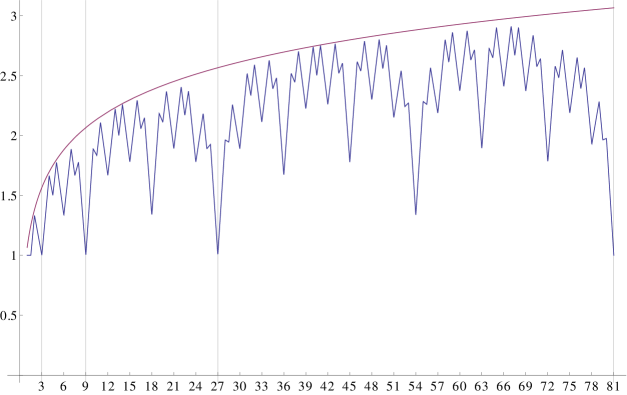
Figure 7: $D(N)=ND_{N}^{*}(Y_{3})$ of the van der Corput sequence in base 3 for $N=1,2,\ldots,81$, in comparison with $N\mapsto\tfrac{\log N}{2\log 3}+\tfrac{3}{4}+\tfrac{\log 2}{2\log 3}$.

For larger bases, the complexity of such generating formulas increases and reduces the interest in searching for them.

2.5 The von Neumann-Kakutani transformation

The van der Corput sequence can also be obtained from the von Neumann-Kakutani transformation. This was first observed by Lambert [86, 87].

The $b$-adic von Neumann-Kakutani transformation $T_{b}:[0,1)\rightarrow[0,1)$ is a piecewise translation map given by

$$T_{b}(x)=x-1+\frac{1}{b^{k}}+\frac{1}{b^{k+1}}\ \ \ \mbox{ for $x\in\left[1-\frac{1}{b^{k}},1-\frac{1}{b^{k+1}}\right)$ with $k=0,1,2,\ldots$.}$$

A plot of $T_{b}$ for $b=2$ is presented in Figure 8. The von Neumann-Kakutani transformation is an ergodic and measure preserving transformation $T_{b}:[0,1)\rightarrow[0,1)$, that is, for every Borel set $A$, $T_{b}A=A$ only if $\lambda(A)=0$ or $\lambda(A)=1$, and $\lambda(T_{b}A)=\lambda(A)$, where $\lambda$ denotes the Lebesgue measure.

Figure 8: The von Neumann-Kakutani transformation for $b=2$.

Likewise, $T_{b}$ can also be constructed inductively with a so-called cutting and stacking construction which is often used in ergodic theory: at first cut $[0,1)$ into $b$ intervals $I_{j}^{(1)}=[\tfrac{j}{b},\tfrac{j+1}{b})$ for $j=0,1,\ldots,b-1$. Define the transformation $T_{b,1}:[0,\tfrac{b-1}{b})\rightarrow[\tfrac{1}{b},1)$ as the translation of $I_{j}^{(1)}$ onto $I_{j+1}^{(1)}$ for $j=0,1,\ldots,b-1$. In the second step cut all intervals $I_{j}^{(1)}$ into $b$ subintervals of the form $I_{j}^{(2)}=[\tfrac{j}{b^{2}},\tfrac{j+1}{b^{2}})$ for $j=0,1,\ldots,b^{2}-1$. Then the transformation $T_{b,2}:[0,\tfrac{b^{2}-1}{b^{2}})\rightarrow[\tfrac{1}{b^{2}},1)$ is the extension of $T_{b,1}$ which translates $I_{b^{2}-b+j}^{(2)}$ onto $I_{b^{2}-b+j+1}^{(2)}$ for $j=0,1,\ldots,b-1$. In this way one can inductively construct a sequence of mappings $T_{b,1},T_{b,2},T_{b,3},\ldots$. The first two steps for $b=2$ are illustrated in Figure 9. Finally the von Neumann-Kakutani transformation is defined as $T_{b}:=\lim_{n\rightarrow\infty}T_{b,n}$. See also [111].

Figure 9: The cutting and stacking construction of $T_{b}$ for $b=2$.

Define the iterates of $T_{b}$ by

$$T_{b}^{n}x=T_{b}T_{b}^{n-1}x\ \ \ \mbox{ for $n\in\mathbb{N}$},$$

where we formally set $T_{b}^{0}x=x$. Then it is easily seen that the orbit of the iterates of $T_{b}$ with starting point $0$ is exactly the van der Corput sequence. For example for $b=2$ we obtain (cf. Figure 8)

$$0\rightarrow 1/2\rightarrow 1/4\rightarrow 3/4\rightarrow 1/8\rightarrow\cdots.$$

It is known that $T_{b}$ is not only ergodic, but it is even uniquely ergodic. From this it follows that the orbit of the iterates of $T_{b}$ is for every starting point $x\in[0,1)$ uniformly distributed modulo 1. Hence the sequence

$$(T_{b}^{n}(x))_{n\geq 0}$$

can be seen as a natural generalization of the van der Corput sequence in base $b$, which is obtained for the choice $x=0$. A proof of this fact and more information in this direction can be found in the excellent survey [61] by Grabner, Hellekalek, and Liardet.

Pagès [113] showed that the orbit of the von Neumann-Kakutani transformation with arbitrary starting point $x\in[0,1)$ has star discrepancy of order of magnitude $O((\log N)/N)$ which is optimal according to Schmidt’s lower bound (6).

2.6 Bounded remainder intervals for the van der Corput sequence

It follows from the lower bound (6) that for every sequence $X$ in $[0,1)$ the sequence $(ND_{N}^{*}(X))_{N\in\mathbb{N}}$ is unbounded as $N\rightarrow\infty$. On the other hand the question arises whether there exist $t\in[0,1)$ for which $N\Delta_{X,N}(t)$ is bounded in $N$. If yes, then an interval $[0,t)$ with this property is called a bounded remainder interval. Bounded remainder intervals or, more generally, bounded remainder sets have been investigated in a series of papers by W.M. Schmidt, see, in particular, [127, 129].

For the van der Corput sequence in base $b$ one can exactly characterize those $t\in[0,1)$ which yield bounded remainder intervals. This was first done by Hellekalek [67].

Theorem 17 (Hellekalek)

An interval $[0,t)$ is a bounded remainder interval for the van der Corput sequence in base $b$ if and only if $t$ is a $b$-adic rational, i.e., $t\in\mathbb{Q}(b^{m})$ for some $m\in\mathbb{N}_{0}$.

The sufficiency of the condition in Theorem 17 is almost trivial. Writing the interval $[0,ab^{-m})$ with $a\in\{0,1,\ldots,b^{m}-1\}$ as the disjoint union $\bigcup_{k=0}^{a-1}[kb^{-m},(k+1)b^{-m})$ it follows from (3) that, for suitable $\theta_{k}\in\{0,1\}$,

$$N\Delta_{Y_{b},N}(ab^{-m})=\sum_{k=0}^{a-1}\left(\left\lfloor\frac{N}{b^{m}}\right\rfloor+\theta_{k}\right)-N\frac{a}{b^{m}}\ll 1.$$

The necessity of the condition needs some investigation for which we refer to [67]. Proofs of the result can also be found in [34, 35, 61]. Quantitative versions of Theorem 17 are given in [27, 34, 35].

We begin with the van der Corput sequence in base $2$ and present the result of [27]. For $t\in[0,1)$ with base 2 representation $t=\tau_{1}/2+\tau_{2}/2^{2}+\cdots$ and $m\in\mathbb{N}$ define

$$f_{t}(m):=\#\{j<m\,:\,\tau_{j}\not=\tau_{j+1}\}\ \ \ \mbox{ and }\ \ \ g_{t}(m):=\frac{1}{2}\sum_{u=0}^{m-1}\|2^{u}t\|.$$

We have the following result.

Theorem 18 (Drmota, Larcher, and Pillichshammer)

Let $t\in[0,1)$ with an infinite base 2 representation. Then for $\varepsilon>0$ we have

$$\lim_{m\rightarrow\infty}\frac{\#\left\{N\leq 2^{m}:(1-\varepsilon)g_{t}(m)<\Delta_{Y_{2},N}(t)<(1+\varepsilon)g_{t}(m)\right\}}{2^{m}}=1.$$

The functions $f_{t}$ and $g_{t}$ are intimately related by the inequality

$$\frac{1}{8}(f_{t}(m)+1)\leq g_{t}(m)\leq\frac{1}{2}(f_{t}(m)+1)\ \ \ \mbox{ for all $t\in[0,1)$ and $m\in\mathbb{N}$,}$$

see [27, Lemma 5]. So we obtain the following corollary.

Corollary 2

Let $t\in[0,1)$ with an infinite base 2 representation. Then for $\varepsilon>0$ we have

$$\lim_{m\rightarrow\infty}\frac{\#\left\{N\leq 2^{m}:(1-\varepsilon)f_{t}(m)<\Delta_{Y_{2},N}(t)\right\}}{2^{m}}=1.$$

Note that Corollary 2 is a strong quantitative version of Theorem 17 (for $b=2$). It follows from [27, Theorem 9] that for every $N\in\mathbb{N}$ we have $|\Delta_{Y_{2},N}(t)|\leq f_{t}(\lfloor\log_{2}N\rfloor)+4$ for every $t\in[0,1)$. This result even holds for more general digital $(0,1)$-sequences over $\mathbb{Z}_{2}$, the definition of which can be found in Section 3.2.

Next, we present another quantitative version of Theorem 17 for generalized van der Corput sequences in base $b$. We first need some notation: For $a\in[0,1)$ and a real $y>0$, let $u_{a}(y,k)$ be the number of occurrences of $k\in\mathbb{Z}_{b}$ among the first $\lfloor y\rfloor+1$ digits in the $b$-adic expansion of $a$,and set $U_{a}(y)=\sum_{k=1}^{b-2}u_{a}(y,k)$. Further we call $V_{a}(y)$ the number of pairs $(0,b-1)$ or $(b-1,0)$ among the first $\lfloor y\rfloor+1$ digits in the $b$-adic expansion of $a$. Let also $\log_{b}$ denote the logarithm to base $b$, i.e., $\log_{b}x=(\log x)/\log b$. The following result is [34, Théorème 1]:

Theorem 19 (Faure)

For any sequence $Y_{b}^{\Sigma}$ we have the following estimates.

1. For every $N\in\mathbb{N}$ we have

   $$\ N|\Delta_{Y_{b}^{\Sigma},N}(a)|\leq\frac{b+4}{4}U_{a}(\log_{b}N)+\frac{(b-1)^{2}}{2b^{2}}V_{a}(\log_{b}N)+\frac{b}{4}+3.$$

2. There exist infinitely many $N\in\mathbb{N}$ such that

   $$N|\Delta_{Y_{b}^{\Sigma},N}(a)|\geq\frac{1}{4}U_{a}(\log_{b}N)+\frac{1}{2}V_{a}(\log_{b}N)-1.$$

As an immediate consequence, we obtain the generalization of Theorem 17 to generalized van der Corput sequences in base $b$. A simpler version exists for $Y_{2}$, see [34, Corollaire 2]. The proof heavily relies on the properties of $\psi$-functions introduced in Section 2.3 for the study of $D_{N}(Y_{b}^{\Sigma}$).

There exists yet another formula for the remainder of van der Corput sequences $Y_{b}$ that draws an interesting parallel between these sequences and $(n\alpha)$-sequences. It was proved (see [34, Théorème 2]) using the famous property of elementary intervals (see Definition 4 in Section 3.2) for the van der Corput sequence.

Theorem 20 (Faure)

For given $a\in[0,1)$ and $N\in\mathbb{N}$, let their $b$-adic expansions be $a=\sum_{j=0}^{\infty}a_{j}b^{-j-1}$ and $N=\sum_{i=0}^{\infty}N_{i}b^{i}$. Put $I(N,a)=\sum_{i=0}^{\infty}\min(N_{i},a_{i})$ and let $W(N,a)$ be the number of pairs $(-,+)$ in the sequence of signs of $(a_{i}-N_{i})_{i\geq 0}$ (disregarding zeros). Then we have

$$N\Delta_{Y_{b},N}(a)=-\sum_{j=0}^{\infty}\sum_{i=0}^{j}N_{i}a_{j}b^{i-j-1}+I(N,a)+W(N,a).$$

The structure of this formula for $Y_{b}$ is exactly the same as that for $(n\alpha)$-sequences obtained in [60, Equation 2.5]. For the sake of completeness, we recall this formula:

For given $x\in[0,1)$ and $N\in\mathbb{N}$, let $x=\sum_{j=1}^{\infty}x_{j}m_{j}$ and $N=\sum_{i=1}^{\infty}y_{i}q_{i}$ (where $y_{i}=0$ for sufficiently large $i$) be their canonical expansions in semi-regular continued fractions (the $(p_{i}/q_{i})$’s approach $\alpha$ and $m_{i}=q_{i}\alpha-p_{i}$). Put $s_{i,j}=q_{i}m_{j}-p_{i}^{j}$, $I(N,x)=\sum_{i=1}^{\infty}\min(x_{i},y_{i})$ and let $W(N,x)$ be the number of pairs $(-,+)$ in the sequence of signs of $(x_{i}-y_{i})_{i\geq 0}$ (disregarding zeros). Then we have

$$N\Delta_{(n\alpha),N}(a)=-\sum_{j=0}^{\infty}\sum_{i=0}^{j}x_{i}y_{j}s_{i,j}+I(N,x)+W(N,x).$$

These formulas underline the relation between van der Corput sequences and $(n\alpha)$-sequences through systems of numeration that permit the precise study of their irregularities of distribution. The simplicity of $b$-adic systems underlying van der Corput sequences as compared to continued fraction systems for $(n\alpha)$-sequences, appears to be the reason for a better understanding, and also a better asymptotic behavior of the former. In the same vein, these two families of sequences are included in a much larger family of sequences of minimal discrepancy, the so-called “self similar sequences” introduced by Borel in [15].

From Theorem 20 it is possible to obtain an improvement of [34, Théorème 1 and Corollaire 2] for the van der Corput sequence $Y_{2}$, see [34, Corollaire 3 and Section 4.5] .

The paper [35] is a variant of Bohl’s lemma for $(n\alpha)$-sequences applied to generalized van der Corput sequences. Bohl’s lemma for $(n\alpha)$-sequences asserts that the remainder on an interval $J\subseteq[0,1)$ only depends the length of $J$. Its very short proof is based on the density of $(n\alpha)$ and on the fact that the counting function does not change under translations of $J$ by $\alpha\pmod{1}$. In contrast to systems of numeration, the variant for $Y_{b}^{\Sigma}$ sequences is much more involved (see [35, Théorème 1]), but it leads to the same property for bounded remainder intervals, i.e., for any $Y_{b}^{\Sigma}$ sequence, $J$ is a bounded remainder interval if and only if ${\rm length}(J)$ is a $b$-adic rational.

2.7 Functions with bounded remainder

The question dealt with in Section 2.6 can be generalized. Let $f:[0,1]\rightarrow\mathbb{R}$ be a Riemann-integrable function with $\int_{0}^{1}f(x)\,\mathrm{d}x=0$ and let $X=(x_{n})_{n\geq 0}$ be a sequence in $[0,1)$. Under which condition on $f$ do we have

$$\sum_{n=0}^{N-1}f(x_{n})\ll 1?$$

The classical example studied in Section 2.6 corresponds to $f(x)=1_{[0,t)}(x)-t$ for $t\in[0,1)$.

In [68] Hellekalek and Larcher studied this question for sequences induced by the von Neumann-Kakutani transformation $T_{b}$ (and also sequences induced by irrational rotations). For $x\in[0,1)$ define

$$G_{N}(x):=\sum_{n=0}^{N-1}f(T_{b}^{n}x).$$

Recall that $(T_{b}^{n}(0))_{n\geq 0}$ is the van der Corput sequence in base $b$ (see Section 2.5).

Theorem 21 (Hellekalek and Larcher)

Let $f\in C^{1}([0,1])$ with $\int_{0}^{1}f(x)\,\mathrm{d}x=0$ and Lipschitz continuous first derivative $f^{\prime}$. Then we have:

1. If $f(0)=f(1)$, then $\sup_{N}|G_{N}(x)|<\infty$ for all $x\in[0,1)$.

2. If $\sup_{N}|G_{N}(x)|<\infty$ for some $x\in[0,1)$, then $f(0)=f(1)$.

3. If $f(1)<f(0)$, then $-\infty<\liminf_{N\rightarrow\infty}G_{N}(0)$ and $\limsup_{N\rightarrow\infty}G_{N}(0)=\infty$.

4. If $f(1)>f(0)$, then $-\infty=\liminf_{N\rightarrow\infty}G_{N}(0)$ and $\limsup_{N\rightarrow\infty}G_{N}(0)<\infty$.

Recall that the Theorem of Rademacher states that every Lipschitz continuous function on an interval is continuously differentiable in almost every point of the interval (in the sense of Lebesgue measure). Hence for the functions considered in Theorem 21 we obtain (by using partial integration) that for $h\not=0$ we have

$$\widehat{f}(h)=\int_{0}^{1}f(x){\rm e}^{-2\pi\mathtt{i}hx}\,\mathrm{d}x=\frac{1}{2\pi\mathtt{i}h}\int_{0}^{1}f^{\prime}(x){\rm e}^{-2\pi\mathtt{i}hx}\,\mathrm{d}x=\frac{1}{(2\pi\mathtt{i}h)^{2}}\int_{0}^{1}f^{\prime\prime}(x){\rm e}^{-2\pi\mathtt{i}hx}\,\mathrm{d}x,$$

and therefore $|\widehat{f}(h)|\ll|h|^{-2}$.

This motivates the following definition: let $\mathcal{F}_{\alpha}$ be the class of all 1-periodic functions $f:\mathbb{R}\rightarrow\mathbb{R}$ with an absolutely convergent Fourier series expansion with $|\widehat{f}(h)|\ll|h|^{-\alpha}$ for all $h\not=0$ and $\int_{0}^{1}f(x)\,\mathrm{d}x=0$. In [23] Dick and Pillichshammer proved the following result for the classical van der Corput sequence in base $b$:

Theorem 22 (Dick and Pillichshammer)

Let $Y_{b}=(y_{n})_{n\geq 0}$ be the van der Corput sequence in base $b$. For $\alpha>1$ we have

$$\left|\sum_{n=0}^{N-1}f(y_{n})\right|\ll 1\quad\ \mbox{ for all $f\in\mathcal{F}_{\alpha}$}.$$ (22)

Furthermore, there exists a function $g\in\mathcal{F}_{1}$ such that

$$\limsup_{N\rightarrow\infty}\left|\sum_{n=0}^{N-1}g(y_{n})\right|=\infty.$$

More accurate results in this direction can be found in [23].

2.8 Subsequences of the van der Corput sequence

In recent years also distribution properties of subsequences (or of index transformed versions) of the van der Corput sequence have been studied. These properties are intimately related to uniform distribution of integer sequences. For $m\in\mathbb{N}$ a sequence $(k_{n})_{n\geq 0}$ of integers is uniformly distributed modulo $m$ if

$$\lim_{N\rightarrow\infty}\frac{\#\{n\in\{0,1,\ldots,N-1\}\ :\ k_{n}\equiv j\pmod{m}\}}{N}=\frac{1}{m}\ \ \ \mbox{ for all $j\in\{0,1,\ldots,m-1\}$}.$$

For information on uniform distribution of integer sequences we refer to [85, Chapter 5, Section 1].

Let $Y_{b}=(y_{n})_{n\geq 0}$ be the van der Corput sequence in base $b$ and let $(k_{n})_{n\geq 0}$ be a sequence in $\mathbb{N}_{0}$. Then it is well known (see, e.g., [75, Remark 4.4]) that the sequence $(y_{k_{n}})_{n\geq 0}$ is uniformly distributed modulo 1 if and only if the sequence $(k_{n})_{n\geq 0}$ is uniformly distributed modulo $b^{d}$ for all $d\in\mathbb{N}_{0}$.

From this insight together with known results on distribution properties of integer sequences (see, e.g., [85] and the references therein) one can obtain the following results which are taken from [75].

Let $Y_{b}=(y_{n})_{n\geq 0}$ denote the van der Corput sequence in base $b$. Then the following statements hold true:

1. The sequence $Y_{b}^{u,v}=(y_{un+v})_{n\geq 0}$ for $(u,v)\in\mathbb{N}\times\mathbb{N}_{0}$ is uniformly distributed modulo 1 if and only if $\gcd(u,b)=1$.

2. For every $\alpha\in\mathbb{N}$, $\alpha\geq 2$, the sequence $(y_{n^{\alpha}})_{n\geq 0}$ is not uniformly distributed modulo 1.

3. Let $p_{n}$, $n\in\mathbb{N}_{0}$, denote the $(n+1)$-st prime number, i.e., $p_{0}=2,p_{1}=3,p_{2}=5,\ldots$. Then the sequence $(y_{p_{n}})_{n\geq 0}$ is not uniformly distributed modulo 1.

4. Let $F_{n}$, $n\in\mathbb{N}_{0}$, denote the $n$-th Fibonacci number, i.e., $F_{0}=0,F_{1}=1$, and $F_{n}=F_{n-1}+F_{n-2}$ for $n\geq 2$. Then the sequence $Y_{b}^{{\rm Fib}}=(y_{F_{n}})_{n\geq 0}$ in base $b$ is uniformly distributed modulo 1 if and only if $b=5^{k}$ for some $k\in\mathbb{N}$.

5. Let $F_{n}$ be as above. Then, in any base $b$, the sequence $(y_{\lfloor\log F_{n}\rfloor})_{n\geq 1}$ is uniformly distributed modulo 1.

6. Let $\xi\in\mathbb{R}\setminus\mathbb{Q}$ or $\xi=1/d$ for some nonzero integer $d$. Then, in any base $b$, the sequence $(y_{\lfloor n\xi\rfloor})_{n\geq 0}$ is uniformly distributed modulo 1.

7. For an integer $q\geq 2$ and $n\in\mathbb{N}_{0}$ let $s_{q}(n)$ denote the $q$-ary sum-of-digits function. Then, in any base $b$, the sequence $Y_{b}^{s_{q}}=(y_{s_{q}(n)})_{n\geq 0}$ is uniformly distributed modulo 1.

In some cases we also have estimates for the star discrepancy of index transformed van der Corput sequences which we collect in the following theorem.

Theorem 23

1. Let $(u,v)\in\mathbb{N}\times\mathbb{N}_{0}$ with $\gcd(u,b)=1$ and let $Y_{b}^{u,v}$ be the van der Corput sequence in base $b$ indexed by the arithmetic progression $un+v$. Then we have

   $$D_{N}^{\ast}(Y_{b}^{u,v})\leq D_{N}^{\ast}(Y_{b}).$$

2. Let $b=5^{\ell}$ and let $Y_{b}^{{\rm Fib}}$ be the van der Corput sequence in base $b$ indexed by the Fibonacci numbers. Then we have

   $$D_{N}^{\ast}(Y_{b}^{{\rm Fib}})\ll_{b}\frac{1}{\sqrt{N}}.$$

3. Let $b,q\geq 2$ be integers and let $Y_{b}^{s_{q}}$ be the van der Corput sequence in base $b$ indexed by the $q$-ary sum-of-digits function $s_{q}$. Then

   $$\frac{1}{\sqrt{\log N}}\ll_{q}D_{N}^{\ast}(Y_{b}^{s_{q}})\ll_{q,b}\frac{\log\log N}{\sqrt{\log N}}.$$

   If $q<14$, then the upper bound can be improved to

   $$D_{N}^{\ast}(Y_{b}^{s_{q}})\ll_{q,b}\frac{1}{\sqrt{\log N}}.$$

4. Let $\alpha\in(0,1)$ and let $Y_{b}^{\alpha}$ be the van der Corput sequence in base $b$ indexed by $\lfloor n^{\alpha}\rfloor$. Then

   $$\frac{1}{N^{\alpha}}\ll_{\alpha}D_{N}^{*}(Y_{b}^{\alpha})\ll_{\alpha}\frac{\log N}{N^{\alpha}}.$$

The first point is [75, Theorem 6.1], the second one is [118, Theorem 2.1]. The third and the fourth points are taken from [81].

2.9 Distribution properties of consecutive elements of the van der Corput sequence

One test for the statistical independence of successive pseudorandom numbers is the so-called serial test. This test can be viewed as a way of measuring the deviation from the property of complete uniform distribution. For a given sequence $X=(x_{n})_{n\geq 0}$ and a fixed dimension $s\geq 2$, consider the overlapping tuples

$$\boldsymbol{x}_{n}=(x_{n},x_{n+1},\ldots,x_{n+s-1})\ \ \ \mbox{ for $n\in\mathbb{N}_{0}$}$$

and consider the discrepancy of the resulting $s$-dimensional sequence $X^{(s)}=(\boldsymbol{x}_{n})_{n\geq 0}$. For a random sequence $Z=(\boldsymbol{z}_{n})_{n\geq 0}$ in $[0,1)^{s}$ the law of the iterated logarithm states that

$$\limsup_{N\rightarrow\infty}\frac{\sqrt{2N}D_{N}^{*}(Z)}{\sqrt{\log\log N}}=1\ \ \ \lambda_{s}^{\infty}{\rm-a.e.},$$

where $\lambda_{s}$ is the $s$-dimensional Lebesgue measure. This serves as a benchmark for the order of magnitude of $D_{N}^{*}(X^{(s)})$. More information on the serial test and further statistical tests for the goodness of fit for the empirical distribution of uniform pseudorandom numbers can be found in the book of Niederreiter [106, Section 7.2].

We now return to the van der Corput sequence. Let $Y_{b}^{(s)}=(\boldsymbol{y}_{n})_{n\geq 0}$ where $\boldsymbol{y}_{n}=(Y_{b}(n),Y_{b}(n+1),\ldots,Y_{b}(n+s-1))$. In [14] Blažeková showed the following result for $s=2$:

Theorem 24 (Blažeková)

For $N\in\mathbb{N}$ we have

$$D_{N}^{*}(Y_{b}^{(2)})=\max\left(\frac{1}{b}\left(1-\frac{1}{b}\right),\frac{1}{4}\left(1-\frac{1}{b}\right)^{2}\right)+O(D_{N}^{*}(Y_{b})).$$

In particular, $\lim_{N\rightarrow\infty}D_{N}^{*}(Y_{b}^{(2)})=\max(\frac{1}{b}(1-\frac{1}{b}),\frac{1}{4}(1-\frac{1}{b})^{2})>0$. Thus the van der Corput sequence $Y_{b}$ does not pass the serial test for $s=2$ and is therefore not a pseudorandom sequence. In [58] Fialova and Strauch showed that every point of $Y_{b}^{(2)}$ lies on the line segment described by the formula

$$y=x-1+\frac{1}{b^{k}}+\frac{1}{b^{k+1}}\ \ \ \mbox{ for $x\in\left[1-\frac{1}{b^{k}},1-\frac{1}{b^{k+1}}\right]$ with $k\in\mathbb{N}_{0}$}$$

and they calculated the limit distribution of the sequence $Y_{b}^{(2)}$.

These findings have been generalized by Aistleitner and Hofer [1] to general $s\geq 2$: let $T_{b}$ denote the $b$-adic von Neumann-Kakutani transformation. Define the map $\gamma:[0,1)\rightarrow[0,1)^{s}$ by setting

$$\gamma(t):=(t,T_{b}t,T_{b}^{2}t,\ldots,T_{b}^{s-1}t)$$

and set

$$\Gamma:=\{\gamma(t)\ :\ t\in[0,1)\}.$$

The Lebesgue measure $\lambda$ on $[0,1)$ induces a measure $\nu$ on $\Gamma$ by setting

$$\nu(A)=\lambda(\{t\ :\ \gamma(t)\in A\})\ \ \mbox{ for $A\subseteq\Gamma$.}$$

Furthermore, $\nu$ induces a measure $\mu$ on $[0,1)^{s}$ by embedding $\Gamma$ into $[0,1)^{s}$, i.e.,

$$\mu(B)=\nu(B\cap\Gamma)\ \ \mbox{ for $B\subseteq[0,1)^{s}$.}$$

Theorem 25 (Aistleitner and Hofer)

The limit measure of $Y_{b}^{(s)}$ is $\mu$.

Note that the measure $\mu$ is a copula on $[0,1]^{s}$ since every distribution function of a multi-dimensional sequence is a copula if all uni-variate projections of the sequence are uniformly distributed modulo 1.

The proof of Theorem 25 in [1] is based on the fact that the van der Corput sequence can be viewed as the orbit of the origin under the ergodic von Neumann-Kakutani transformation (see Section 2.5).

Recently Lertchoosakul and Nair [97] studied the same question for sequences of the form

$$(Y_{b}(k_{n}+n_{1}),\ldots,Y_{b}(k_{n}+n_{s}))_{n\geq 0},$$

where $(n_{1},\ldots,n_{s})$ is a fixed $s$-tuple of non-negative integers and where the integer sequence $(k_{n})_{n\geq 0}$ is Hartmann uniformly distributed on $\mathbb{Z}$. It is shown in [97] that the asymptotic distribution function exists and is a copula.

3 Generalizations and variants of the van der Corput sequence

Several authors have studied different ways of generalizing or modifying the van der Corput sequence. In this section, we describe some of the most important variants.

3.1 Symmetrized generalized van der Corput sequences

One way to overcome the defect that, compared to the lower bound in (7), the van der Corput sequence does not have optimal order of $L_{p}$-discrepancy is based on a process which was initially introduced by Davenport for $(n\alpha)$-sequences (see [17] or [28, Theorem 1.75]). This method is also known as Davenport’s reflection principle. Later Proinov [120], who named the process symmetrization of a sequence, obtained the same result with generalized van der Corput sequences.

Definition 3

A sequence $Y=(y_{n})_{n\geq 0}$ is called symmetric if for all $n\in\mathbb{N}_{0}$, one has $y_{2n}+y_{2n+1}=1$. A symmetric sequence $Y=(y_{n})_{n\geq 0}$ is said to be produced by a sequence $X=(x_{n})_{n\geq 0}$ if for all $n\in\mathbb{N}_{0}$ one has $y_{2n}=x_{n}$ or $y_{2n+1}=x_{n}$. In this case, the sequence $Y$ is called a symmetrized version of $X$ and is denoted as $Y=\widetilde{X}$.

Two years after Proinov, Faure [37, Théorème 3] obtained an exact formula for the $L_{2}$-discrepancy of the symmetrized sequence $\widetilde{Y}_{2}$ of the van der Corput sequence $Y_{2}$ (for short, the symmetrized van der Corput sequence). The proof is based on the descent method (see Section 2.4) worked out for the first time for that study of $Y_{2}$ and $\widetilde{Y}_{2}$.

We remark that the symmetrized van der Corput sequence in base 2 can also be obtained with the help of the tent-transformation $\Psi:[0,1]\rightarrow[0,1]$, given by $\Psi(x)=1-|2x-1|$, which is a Lebesgue measure preserving function. If $Y_{2}=(y_{n})_{n\geq 0}$ denotes the van der Corput sequence in base 2, then

$$\widetilde{Y}_{2}=\Psi(Y_{2})=(\Psi(y_{n}))_{n\geq 0}.$$

Theorem 26 (Faure)

For any positive integers $m$ and $N$ such that $1\leq N\leq 2^{m}$, we have

$$(NL_{2,N}(\widetilde{Y}_{2}))^{2}=\sum_{j=1}^{m}(1-2\|2^{j}Y_{2}(N+1)\|)\ \left\|\frac{N}{2^{j}}\right\|^{2}+\frac{N^{2}}{3\cdot 4^{m}}\cdot$$

Corollary 3

The preceding theorem implies the following formula and estimate:

$$t_{2}(\widetilde{Y}_{2})=\inf_{m\geq 1}\max_{1\leq N\leq 2^{m}}\left(\frac{1}{m\log 2}\sum_{j=1}^{m}(1-2\|2^{j}Y_{2}(N+1)\|)\ \left\|\frac{N}{2^{j}}\right\|^{2}\right)$$

and

$$0.089\ldots=\frac{421}{6750\log 2}\leq t_{2}(\widetilde{Y}_{2})<0.103.$$

Numerical computations suggest that the lower bound in Corollary 3 is the exact value of $t_{2}(\widetilde{Y}_{2})$.

The proof of the preceding result is based on the descent method which permits a very precise study of the $L_{2}$-discrepancy of $\widetilde{Y}_{2}$, but which (until now) is ineffective for the $L_{p}$-discrepancy. The optimal order of $L_{2,N}(\widetilde{Y}_{2})$ was also shown in [91] by means of a Walsh series expansion of the local discrepancy and Parseval’s identity. On the other hand, quite recently, Kritzinger and Pillichshammer [84] obtained a general optimal estimation for the $L_{p}$-discrepancy of $\widetilde{Y}_{2}$ (with non-explicit constants) by means of strong analytic tools. This is a new illustration of (at least) two complementary approaches in discrepancy theory that are source a of emulation and progress (see also Sections 2.5 and 2.6).

Theorem 27 (Kritzinger and Pillichshammer)

For every $p\in[1,\infty)$ we have

$$L_{p,N}(\widetilde{Y}_{2})\ll_{p}\frac{\sqrt{\log{N}}}{N}.$$

We conjecture that an analogous result to Theorem 27 also holds for general bases $b$ (this is work in progress). The proof of Theorem 27 is based on dyadic Haar functions and on Littlewood-Paley theory. We sketch the basic ideas:

A dyadic interval of length $2^{-j}$, $j\in{\mathbb{N}}_{0},$ in $[0,1)$ is an interval of the form

$$I=I_{j,m}:=\left[\frac{m}{2^{j}},\frac{m+1}{2^{j}}\right)\ \ \mbox{for }\ m=0,1,\ldots,2^{j}-1.$$

We also define $I_{-1,0}=[0,1)$. The left and right halves of $I=I_{j,m}$ are the dyadic intervals $I^{+}=I_{j,m}^{+}=I_{j+1,2m}$ and $I^{-}=I_{j,m}^{-}=I_{j+1,2m+1}$, respectively. The Haar function $h_{I}=h_{j,m}$ with support $I$ is the function on $[0,1)$ which is $+1$ on the left half of $I$, $-1$ on the right half of $I$ and 0 outside of $I$. The $L_{\infty}$-normalized Haar system consists of all Haar functions $h_{j,m}$ with $j\in{\mathbb{N}}_{0}$ and $m=0,1,\ldots,2^{j}-1$ together with the indicator function $h_{-1,0}$ of $[0,1)$. Normalized in $L_{2}([0,1))$ we obtain the orthonormal Haar basis of $L_{2}([0,1))$.

The Haar coefficients of a function $f\in L_{p}([0,1))$ are defined as

$$\mu_{j,m}(f):=\langle f,h_{j,m}\rangle=\int_{0}^{1}f(t)h_{j,m}(t)\,\mathrm{d}t\ \ \ \mbox{for $j\in\mathbb{N}_{-1}$ and $m\in\mathbb{D}_{j}$},$$

where we use the abbreviations $\mathbb{N}_{-1}:=\mathbb{N}_{0}\cup\{-1\}$, $\mathbb{D}_{j}:=\{0,1,\dots,2^{j}-1\}$ for $j\in\mathbb{N}_{0}$, and $\mathbb{D}_{-1}:=\{0\}$.

In order to prove Theorem 27 we apply the Littlewood-Paley inequality which involves the square function

$$S(f):=\left(\sum_{j\in\mathbb{N}_{-1}}\sum_{m\in\mathbb{D}_{j}}2^{2\max\{0,j\}}\,\langle f,h_{j,m}\rangle^{2}\,{\mathbf{1}}_{I_{j,m}}\right)^{1/2}\ \ \ \mbox{ for $f\in L_{p}([0,1))$.}$$

Lemma 3 (Littlewood-Paley inequality)

Let $p\in(1,\infty)$. Then there exist $c_{p},C_{p}>0$ such that for every $f\in L_{p}([0,1))$ we have

$$c_{p}\|f\|_{L_{p}}\leq\|S(f)\|_{L_{p}}\leq C_{p}\|f\|_{L_{p}}.$$

So it remains to find good estimates for the Haar coefficients $\langle f,h_{j,m}\rangle$ when $f$ is the local discrepancy of the first $N$ terms of $\widetilde{Y}_{2}$. Let $\mu_{j,m}^{N,{\rm sym}}:=\langle\Delta_{\widetilde{Y}_{2},N},h_{j,m}\rangle$. The following estimate was shown in [84]:

Lemma 4

For $j\in\mathbb{N}_{0}$ and $m\in\mathbb{D}_{j}$ we have

$$|\mu_{j,m}^{N,{\rm sym}}|\left\{\begin{array}[]{ll}\leq\frac{1}{2^{j-1}}\frac{1}{N}&\mbox{ if }j<\lceil\log_{2}{N}\rceil,\\ \\ =2^{-2j-2}&\mbox{ if }j\geq\lceil\log_{2}{N}\rceil.\end{array}\right.$$

Furthermore we also have

$$|\mu_{-1,0}^{N,{\rm sym}}|=\begin{cases}0&\mbox{if }N=2M,\\ \left|\frac{1}{2N}-\frac{Y_{2}(M)}{N}\right|\leq\frac{1}{2N}\ &\mbox{if }N=2M+1.\end{cases}$$ (23)

Equation (23) is the most crucial part in the proof of Theorem 27. It shows how the symmetrization trick keeps the Haar coefficient $\mu_{-1,0}^{N,{\rm sym}}$ small enough in order to achieve the optimal $L_{p}$-discrepancy rate. For the non-symmetrized van der Corput sequence the corresponding Haar coefficient is at least of order $(\log N)/N$ for infinitely many $N\in\mathbb{N}$ which causes the large $L_{p}$-discrepancy of $Y_{2}$.

With the ingredients of Lemmas 3 and 4 one can derive the result in Theorem 27 (cf. [84]):

Proof of Theorem 27. Using Lemma 3 with $f=\Delta_{\widetilde{Y}_{2},N}$ we have

$$L_{p,N}(\widetilde{Y}_{2}) \ll_{p} \|S(\Delta_{\widetilde{Y}_{2},N})\|_{L_{p}}$$

$$= \left\|\left(\sum_{j\in\mathbb{N}_{-1}}\sum_{m\in\mathbb{D}_{j}}2^{2\max\{0,j\}}\,(\mu_{j,m}^{N,{\rm sym}})^{2}\,{\mathbf{1}}_{I_{j,m}}\right)^{1/2}\right\|_{L_{p}}$$

$$= \left\|\sum_{j\in\mathbb{N}_{-1}}2^{2\max\{0,j\}}\sum_{m\in\mathbb{D}_{j}}\,(\mu_{j,m}^{N,{\rm sym}})^{2}\,{\mathbf{1}}_{I_{j,m}}\right\|_{L_{p/2}}^{1/2}$$

$$\leq \left(\sum_{j\in\mathbb{N}_{-1}}2^{2\max\{0,j\}}\left\|\sum_{m\in\mathbb{D}_{j}}\,(\mu_{j,m}^{N,{\rm sym}})^{2}\,{\mathbf{1}}_{I_{j,m}}\right\|_{L_{p/2}}\right)^{1/2},$$

where we used Minkowski’s inequality for the $L_{p/2}$-norm. Now Lemma 4 gives

$$\sum_{j\in\mathbb{N}_{-1}}2^{2\max\{0,j\}}\left\|\sum_{m\in\mathbb{D}_{j}}\mu_{j,m}^{2}\,{\mathbf{1}}_{I_{j,m}}\right\|_{L_{p/2}}\leq \frac{1}{4N^{2}}\|\boldsymbol{1}_{\left[0,1\right)}\|_{L_{p/2}}+\frac{4}{N^{2}}\sum_{j=0}^{\lceil\log_{2}{N}\rceil-1}\left\|\sum_{m\in\mathbb{D}_{j}}\,{\mathbf{1}}_{I_{j,m}}\right\|_{L_{p/2}}$$

$$+\frac{1}{16}\sum_{j=\lceil\log_{2}{N}\rceil}^{\infty}2^{-2j}\left\|\sum_{m\in\mathbb{D}_{j}}\,{\mathbf{1}}_{I_{j,m}}\right\|_{L_{p/2}}$$

$$\leq \frac{1}{4N^{2}}+\frac{4}{N^{2}}(\log_{2}{N}+1)+\frac{1}{12}\frac{1}{4^{\lceil\log_{2}{N}\rceil}}\ll\frac{\log{N}}{N^{2}},$$

where we regarded the fact that $\sum_{m\in\mathbb{D}_{j}}\,{\mathbf{1}}_{I_{j,m}}=1$ for a fixed $j\in\mathbb{N}_{0}$. $\hfill\Box\vspace{0.5cm}$

A general approach to obtain optimal upper bounds for the $L_{2}$-discrepancy of generalized van der Corput sequences in any base $b$ comes from an inequality between $L_{2,N}(\widetilde{X})$ and the diaphony $F_{N}(X)$, see [122, Theorem A] and also [16, Section 4.2.3]:

Theorem 28 (Proinov and Grozdanov)

There exist two constants $a_{1}$ and $a_{2}$ such that

$$(NL_{2,N}(\widetilde{X}))^{2}\leq\left(\frac{1}{\pi}\left\lfloor\frac{N}{2}\right\rfloor F_{\left\lfloor N/2\right\rfloor}(X)+a_{1}\right)^{2}+a_{2}^{2}.$$

Corollary 4

The asymptotic behavior of $L_{2,N}(\widetilde{Y}_{b}^{\Sigma})$ is related to the asymptotic behavior of $F_{N}(Y_{b}^{\Sigma})$ by the inequality

$$t_{2}(\widetilde{Y}_{b}^{\Sigma})=\limsup_{N\rightarrow\infty}\frac{(NL_{2,N}(\widetilde{Y}_{b}^{\Sigma}))^{2}}{\log N}\leq\frac{1}{\pi}f(Y_{b}^{\Sigma}).$$

The state of the art regarding the optimal constant $t_{2}=\inf_{X}(t_{2}(X))$ is the following (see the end of Section 2.3 for the definition). From Corollary 4, we have the constants $t_{2}=f/\pi^{2}$ resulting from state of the art for the constants $f$ hence, for short, $t_{2}<0.134$ in base 19 by Chaix and Faure in 1993 and $t_{2}<0.116$ in base 57 by Pausinger and Schmid in 2010. However, these values remain larger than the bound obtained by Faure in 1990 for base 2 with an exact formula for $t_{2}(\widetilde{Y}_{2})$, see Corollary 3, namely $t_{2}<0.103$. This means that

$$0.051599\ldots\leq\inf_{X}\limsup_{N\rightarrow\infty}\frac{NL_{2,N}(X)}{\sqrt{\log N}}\leq 0.32093\ldots,$$

where the infimum is extended over all sequences $X$ in $[0,1)$. Note that the lower and upper bounds in the latter equation roughly differ by a factor of 6.

3.2 $(0,1)$-sequences and NUT sequences

General remarks on $(0,1)$-sequences.

We already observed in Section 2 that for every $m\in\mathbb{N}_{0}$ and $k\in\{0,1,\ldots,b^{m}-1\}$ exactly one of $b^{m}$ consecutive elements of the van der Corput sequence in base $b$ belongs to the so-called $b$-adic elementary interval $[\frac{k}{b^{m}},\frac{k+1}{b^{m}})$. This fundamental property of the van der Corput sequence is the basis of the following definition which goes back to Niederreiter [106]; see also [24].

Definition 4

A sequence $(x_{n})_{n\geq 0}$ in the unit interval $[0,1)$ is called a $(0,1)$-sequence in base $b$ if every elementary interval $E$ of the form $[\frac{k}{b^{m}},\frac{k+1}{b^{m}})$, with $m\in\mathbb{N}_{0}$ and $k\in\{0,1,\ldots,b^{m}-1\}$, contains exactly one element of the point set

$$\{x_{n}\,:\,lb^{m}\leq n\leq(l+1)b^{m}-1\}\ \ \ \mbox{ for every $l\in\mathbb{N}_{0}$.}$$

Of course, for every $b\geq 2$ the van der Corput sequence $Y_{b}$ is a $(0,1)$-sequence in base $b$.

To take into account important special cases, it is convenient to work with a slightly modified definition. To this end define for every $x\in[0,1]$ and for every $m\in\mathbb{N}$ the $m$-truncated expansion of $x$ by $[x]_{b,m}=\sum_{i=1}^{m}\xi_{i}b^{-i}$, where $x=\sum_{i=1}^{\infty}\xi_{i}b^{-i}$ is the $b$-adic expansion of $x$, with the possibility that $\xi_{i}=b-1$ for all but finitely many $i$. Then a sequence $(x_{n})_{n\geq 0}$ in the unit interval $[0,1)$ is called a $(0,1)$-sequence in base $b$ in the broad sense if every elementary interval $E$ of the form $[\frac{k}{b^{m}},\frac{k+1}{b^{m}})$, with $m\in\mathbb{N}_{0}$ and $k\in\{0,1,\ldots,b^{m}-1\}$, contains exactly one element of the point set

$$\{[x_{n}]_{b,m}\,:\,lb^{m}\leq n\leq(l+1)b^{m}-1\}\ \ \ \mbox{ for every $l\in\mathbb{N}_{0}$.}$$

Faure [42, Proposition 3.1] showed that every generalized van der Corput sequence in base $b$ is a $(0,1)$-sequence in base $b$ in the broad sense. The truncation is required for sequences $Y_{b}^{\Sigma}$ where $\sigma_{r}(0)=b-1$ for all sufficiently large $r$.

It is known that among all $(0,1)$-sequences in base $b$ the classical van der Corput sequence in base $b$ has the worst star discrepancy. This was first shown by Pillichshammer [117] for $b=2$ and later generalized by Kritzer [77] to general $b$ and next by Faure [42] to $(0,1)$-sequences in the broad sense (a further extension to $(t,1)$-sequences in the broad sense is given in [49], see Section 4.3 for the meaning of $t$).

Theorem 29 (Faure, Kritzer, and Pillichshammer)

Let $X_{b}$ be an arbitrary $(0,1)$-sequence in base $b$ in the broad sense and let $Y_{b}$ be the van der Corput sequence in base $b$. Then we have

$$D_{N}^{*}(X_{b})\leq D_{N}^{*}(Y_{b}).$$

In particular,

$$\limsup_{N\rightarrow\infty}\sup_{X_{b}}\frac{ND_{N}^{\ast}(X_{b})}{\log N}=\frac{\alpha_{b,{\rm id}}}{\log b},$$

where $\alpha_{b,{\rm id}}$ is defined as in (15) and where the supremum is extended over all $(0,1)$-sequences $X_{b}$ in base $b$.

For the construction of a $(0,1)$-sequence in base $b$ one frequently uses the digital method which is based on the action of infinite $\mathbb{N}\times\mathbb{N}$ matrices, over a finite commutative ring with identity and with $b$ elements, on the $b$-adic digits of $n\in\mathbb{N}_{0}$. For simplicity, here we only present the case where $b$ is a prime power and where $R=\mathbb{F}_{b}$, the finite field with $b$ elements. For the general case ($b\geq 2$ and $R$ an arbitrary commutative ring with identity and with $b$ elements) we refer to [104, 106]. We also require a bijection $\varphi:\mathbb{Z}_{b}\rightarrow\mathbb{F}_{b}$ with the property that $\varphi(0)=0$.

Definition 5

Let $b$ be a prime power. Choose an $\mathbb{N}\times\mathbb{N}$ matrix $C=(c_{r,k})_{r,k\geq 0}$ with entries in $\mathbb{F}_{b}$ such that for any $m\in\mathbb{N}$ every left upper $m\times m$ sub-matrix of $C$ is non-singular. Then the sequence $X_{b}^{C}=(x_{n})_{n\geq 0}$ defined by

$$x_{n}=\sum_{r=0}^{\infty}\frac{\varphi^{-1}(\xi_{n,r})}{b^{r+1}},\quad{\rm where}\quad\xi_{n,r}=\sum_{k=0}^{\infty}c_{r,k}\varphi(n_{k}),$$ (24)

and where the $n_{k}\in\mathbb{Z}_{b}$ are the $b$-adic digits of $n$, is called a digital $(0,1)$-sequence over $\mathbb{F}_{b}$. Note that the second summation in (24) is finite and performed in $\mathbb{F}_{b}$, but the first one can be infinite with the possibility that $\varphi^{-1}(\xi_{n,r})=b-1$ for all but finitely many $r$.

If $b$ is a prime number, then we identify $\mathbb{F}_{b}$ with $\mathbb{Z}_{b}$ equipped with addition and multiplication modulo $b$. In this case we choose for $\varphi$ the identity. We then obtain the original van der Corput sequence $Y_{b}$ with the $\mathbb{N}\times\mathbb{N}$ identity matrix $I$, i.e., we have $Y_{b}=X_{b}^{I}$.

It is well known that a digital $(0,1)$-sequence over $\mathbb{F}_{b}$ is a $(0,1)$-sequence in base $b$ if $C$ is such that for all $k\geq 0$ we have $c_{r,k}=0$ for $r$ sufficiently large (see [24, 96, 106]), but in any case it is a $(0,1)$-sequence in base $b$ in the broad sense (see [42]). The truncation is required for sequences $X_{b}^{C}$ in the case when the matrix $C$ yields digits $\varphi^{-1}(x_{n,r})=b-1$ for all sufficiently large $r$.

NUT digital $(0,1)$-sequences.

An important special case of digital $(0,1)$-sequences is obtained when the associated matrix $C$ is a non-singular upper triangular (NUT) matrix. In this case the first summation in (24) is finite as well. These sequences are called NUT digital $(0,1)$-sequences over $\mathbb{F}_{b}$. In [39] Faure proved formulas in the vein of Theorems 7 and 8 for the different notions of discrepancies of NUT digital $(0,1)$-sequences over $\mathbb{F}_{b}$ (where $b$ is a prime number).

To recall these formulas we first need to introduce some definitions to deal with NUT digital $(0,1)$-sequences. Let again $b$ be a prime number, identify $\mathbb{F}_{b}$ with $\mathbb{Z}_{b}$, and let $\varphi={\rm id}$. The symbol $\uplus$ is used to denote the translated (or shifted) permutation corresponding to a given permutation $\sigma\in\mathfrak{S}_{b}$ by an element $v\in{\mathbb{F}}_{b}$ in the following sense:

$$(\sigma\uplus v)(i):=\sigma(i)+v\pmod{b}\quad{\rm for\ all}\quad i\in{\mathbb{F}}_{b},$$

and for any $r\in\mathbb{N}_{0}$ we introduce the quantity

$$\theta_{r}(N):=\displaystyle\sum_{k=r+1}^{\infty}c_{r,k}N_{k}\pmod{b},$$

where the $N_{k}$’s are the $b$-adic digits of $N$. Note that $N_{k}=0$ for all $k\geq m$ if $0\leq N<b^{m}$, thus $\theta_{r}(N)=0$ for all $r\geq m-1$ in this case. Finally, for $r\geq 0$, we define the permutation $\delta_{r}$ by $\delta_{r}(i):=c_{r,r}i\pmod{b}$ for $i\in\mathbb{F}_{b}$ and for future use we set $\Delta:=(\delta_{r})_{r\geq 0}$. We can now formulate the following result.

Theorem 30 (Faure)

Let $X_{b}^{C}$ be a NUT digital $(0,1)$-sequence over $\mathbb{F}_{b}$ with prime $b$. Then, using the notation introduced in Section 2.3, for any $N\in\mathbb{N}$ we have

$$D_{N}^{+}(X_{b}^{C})=\frac{1}{N}\sum_{j=1}^{\infty}\psi_{b}^{\delta_{j-1}\uplus\theta_{j-1}(N),+}\left(\frac{N}{b^{j}}\right),$$

$$D^{-}_{N}(X_{b}^{C})=\frac{1}{N}\sum_{j=1}^{\infty}\psi_{b}^{\delta_{j-1}\uplus\theta_{j-1}(N),-}\left(\frac{N}{b^{j}}\right),$$

$$D_{N}(X_{b}^{C})=\frac{1}{N}\sum_{j=1}^{\infty}\psi_{b}^{\delta_{j-1}}\left(\frac{N}{b^{j}}\right),$$

$$D_{N}^{\ast}(X_{b}^{C})=\max(D^{+}_{N}(X_{b}^{C}),D^{-}_{N}(X_{b}^{C})),$$

$$(NF_{N}(X_{b}^{C}))^{2}=\frac{4\pi^{2}}{b^{2}}\sum_{j=1}^{\infty}\chi_{b}^{\sigma_{j-1}}\left(\frac{N}{b^{j}}\right),$$

$$(NL_{2,N}(X_{b}^{C}))^{2}=\\ \frac{1}{b}\sum_{j=1}^{\infty}\phi_{b}^{\delta_{j-1}\uplus\theta_{j-1}(N)}\left(\frac{N}{b^{j}}\right)+\frac{1}{b^{2}}\sum_{i\neq j}\varphi_{b}^{\delta_{i-1}\uplus\theta_{i-1}(N)}\left(\frac{N}{b^{i}}\right)\varphi_{b}^{\delta_{j-1}\uplus\theta_{j-1}(N)}\left(\frac{N}{b^{j}}\right).$$

The formulas in Theorem 30 for $D_{N}$ and $F_{N}$ show that digital $(0,1)$-sequences generated by NUT matrices having the same diagonal entries have the same extreme discrepancy and the same diaphony. Therefore, for $D_{N}$ and $F_{N}$ generalized van der Corput sequences and NUT digital $(0,1)$-sequences have the same behavior, i.e., $D_{N}(X_{b}^{C})=D_{N}(Y_{b}^{\Delta})$ and $F_{N}(X_{b}^{C})=F_{N}(Y_{b}^{\Delta})$. This is a remarkable feature of NUT digital $(0,1)$-sequences that yields the asymptotic behavior of $D_{N}(X_{b}^{C})$ and $F_{N}(X_{b}^{C})$, directly using the results in Section 2.3.

For $D_{N}^{+}$, $D_{N}^{-}$, $D_{N}^{*}$, and $L_{2,N}$, the formulas are similar to those for generalized van der Corput sequences, but the situation is more complicated because of the quantity $\theta_{j-1}(N)$ which depends on $N$, via the $b$-adic expansion of $N-1$, and on the NUT generator matrix $C$, via its entries strictly above the diagonal. Very few results are available, for example Theorem 32 below for $b=2$, or loose bounds for $L_{2,N}$ in a very special case in base $b$ by Grozdanov [62].

Generalization of NUT digital $(0,1)$-sequences.

A further generalization of NUT digital $(0,1)$-sequences, in relation with the search for best possible lower bounds for the star discrepancy, has recently been given by Faure and Pillichshammer in [55]. The resulting family in arbitrary integer bases—named NUT $(0,1)$-sequences over $\mathbb{Z}_{b}$—include both, generalized van der Corput sequences $Y_{b}^{\Sigma}$, and NUT digital $(0,1)$-sequences $X_{b}^{C}$. So far, this is the most general family of van der Corput type sequences.

The idea is to put arbitrary permutations in place of the diagonal entries of the NUT matrix $C$ defining a NUT digital $(0,1)$-sequence:

Definition 6

For any integer $b\geq 2$, let $\Sigma=(\sigma_{r})_{r\geq 0}\in\mathfrak{S}_{b}^{\mathbb{N}}$ and let $C=(c_{r}^{k})_{r\geq 0,k\geq r+1}$ be a strict upper triangular matrix with entries in $\mathbb{Z}_{b}$. Then, for $n\in\mathbb{N}_{0}$, the $n$-th element of the sequence $X_{b}^{\Sigma,C}=(x_{n})_{n\geq 0}$ is defined by

$$x_{n}=\sum_{r=0}^{\infty}\frac{x_{n,r}}{b^{r+1}}\quad{\rm with}\quad x_{n,r}=\sigma_{r}(n_{r})+\sum_{k=r+1}^{\infty}c_{r}^{k}n_{k}\pmod{b},$$ (25)

where the $n_{k}$’s are the $b$-adic digits of $n$. We call $X_{b}^{\Sigma,C}$ a NUT $(0,1)$-sequence over $\mathbb{Z}_{b}$.

If all entries of $C$ are zero, then we have $X_{b}^{\Sigma,C}=Y_{b}^{\Sigma}$, the generalized van der Corput sequences. If $\sigma_{r}=\delta_{r}$ for all $r\geq 0$ with $\delta_{r}$ as in Theorem 30, then we have $X_{b}^{\Sigma,C}=X_{b}^{C^{\prime}}$, the NUT digital $(0,1)$-sequence where $C^{\prime}=(c_{r}^{k})_{r\geq 0,k\geq r}$ is obtained from $C$ by putting invertible entries $c_{r}^{r}\in\mathbb{Z}_{b}$ on the diagonal.

Every NUT $(0,1)$-sequence over $\mathbb{Z}_{b}$ is a $(0,1)$-sequence in the broad sense (the proof works like for generalized van der Corput sequences in [42]).

It is quite remarkable that Theorem 30 for NUT digital $(0,1)$-sequences in prime base $b$ is still valid for this generalization (the basic trick is to keep bijections of $\mathbb{Z}_{b}$ “on the diagonal”, which is the only place where computing inverses is required, all other operations concerning entries above the diagonal are performed in the ring $\mathbb{Z}_{b}$):

Theorem 31 (Faure and Pillichshammer)

Let $X_{b}^{\Sigma,C}$ be a NUT $(0,1)$-sequence over $\mathbb{Z}_{b}$ where $b\geq 2$ is an integer. Then the results of Theorem 30 are still valid for $X_{b}^{\Sigma,C}$ with permutations $\sigma_{r}$ replacing the permutations $\delta_{r}$.

The proof of Theorem 31 is rather complex and requires a lot of prerequisites, but it follows closely the proofs of [39, Theorems 1–4]. See [55] for a sketch where differences between both proofs are pointed out.

Some applications of Theorem 31 will be given later. We now turn to some special digital $(0,1)$-sequences over $\mathbb{F}_{2}$.

Special digital $(0,1)$-sequences over $\mathbb{F}_{2}$.

In base $b=2$ one knows a NUT digital $(0,1)$-sequence over $\mathbb{F}_{2}$ with smaller star discrepancy than the van der Corput sequence in base $2$. This sequence was given in [117, Theorem 3].

Theorem 32 (Pillichshammer)

For the star discrepancy of the NUT digital $(0,1)$-sequence over $\mathbb{F}_{2}$ generated by the matrix

$$C_{1}:=\left(\begin{array}[]{lllll}1&1&1&1&\ldots\\ 0&1&1&1&\ldots\\ 0&0&1&1&\ldots\\ 0&0&0&1&\ldots\\ \vdots&\vdots&\vdots&&\ddots\end{array}\right)$$

we have

$$0.2885\ldots=\frac{1}{5\log 2}\leq\limsup_{N\rightarrow\infty}\frac{ND_{N}^{*}(X_{2}^{C_{1}})}{\log N}\leq\frac{5099}{22528\log 2}=0.3265\ldots.$$

The next example from [42] shows that the van der Corput sequence in base 2, is not the worst distributed with respect to the extreme discrepancy $D_{N}$ among digital $(0,1)$-sequences in base $2$ (but $Y_{2}$ is the worst distributed with respect to $D_{N}$, $D_{N}^{*}$, $F_{N}$ and $L_{2,N}$ among NUT digital $(0,1)$-sequences in base $b$, see Theorem 35 below).

Theorem 33 (Faure)

Let $C_{2}$ be the matrix

$$C_{2}:=\begin{pmatrix}1&0&0&0&\cdots\cr\vskip 3.0pt\cr 1&1&0&0&\cdots\cr\vskip 3.0pt\cr 1&0&1&0&\cdots\cr\vskip 3.0pt\cr 1&0&0&1&\cdots\cr\vskip 3.0pt\cr\vdots&\vdots&\vdots&\vdots&\ddots\cr\end{pmatrix}.$$

Then, for any $N\in\mathbb{N}$ we have

$$2D_{N}(Y_{2})-\frac{5}{2N}\leq D_{N}(X_{2}^{C_{2}})\leq 2D_{N}(Y_{2})\quad{\it and}$$

$$D^{*}_{N}(Y_{2})-\frac{3}{2N}\leq D^{*}_{N}(X_{2}^{C_{2}})\leq D^{*}_{N}(Y_{2})=D_{N}(Y_{2}).$$

Moreover, the sequence $X_{2}^{C_{2}}$ is the worst distributed among all $(0,1)$-sequences in base $2$ (in the broad sense) with respect to the extreme discrepancy $D_{N}$.

The sequence $X_{2}^{C_{2}}$ was already considered by Larcher and Pillichshammer [91] to show that there exists a symmetrized version of a digital $(0,1)$-sequence in base 2, namely $\widetilde{X}_{2}^{C_{2}}$, that does not have optimal order of $L_{2}$-discrepancy. It should be remarked that $X_{2}^{C_{2}}=\widetilde{Y}_{2}$. We see here that $X_{2}^{C_{2}}$ has about the same star discrepancy as $Y_{2}$, but its extreme discrepancy $D_{N}$ is about twice $D_{N}(Y_{2})$ and it is the worst among all $(0,1)$-sequences in base 2. Thus, this sequence appears to be one with bad distribution properties (recall that the symmetrized sequence of $Y_{2}$ has optimal order of $L_{2}$-discrepancy).

The $L_{2}$-discrepancy of NUT digital $(0,1)$-sequences over $\mathbb{F}_{2}$ is studied in [27].

Theorem 34 (Drmota, Larcher, and Pillichshammer)

Let $X_{2}^{C}$ be a NUT digital $(0,1)$-sequence over $\mathbb{F}_{2}$ generated by a NUT matrix $C$ and let $Y_{2}$ be the van der Corput sequence in base 2. Then we have

$$(NL_{2,N}(X_{2}^{C}))^{2}\leq(NL_{2,N}(Y_{2}))^{2}\leq\left(\frac{\log N}{6\log 2}\right)^{2}+O(\log N)$$ (26)

and

$$\limsup_{N\rightarrow\infty}\sup_{X_{2}^{C}}\frac{NL_{2,N}(X_{2}^{C})}{\log N}=\frac{1}{6\log 2}$$ (27)

where the supremum is extended over all NUT digital $(0,1)$-sequences $X_{2}^{C}$ over $\mathbb{F}_{2}$. Furthermore, for the matrix $C_{1}$ defined in Theorem 32 there exists a real $c>0$ such that

$$L_{2,N}(X_{2}^{C_{1}})\geq c\frac{\log N}{N}\ \ \ \mbox{ for infinitely many $N\in\mathbb{N}$.}$$

For central limit theorems for the discrepancy of NUT digital $(0,1)$-sequences over $\mathbb{F}_{2}$ we refer to [27, Theorems 5 and 6].

The worst distributed sequence among NUT $(0,1)$-sequences $X_{b}^{\Sigma,C}$.

Due to the theory of $\varphi_{b}$-functions for the study of van der Corput sequences and their generalizations, it is possible to bound the discrepancies and the diaphony of sequences obtained.

In [40, Lemmas 1–3], the following bounds were obtained:

$$\psi_{b}^{\sigma}\leq\psi_{b}^{\rm id},\ \ \ |\varphi_{b}^{\sigma}|\leq\varphi_{b}^{\rm id}\ \mbox{ and }\ \chi_{b}^{\sigma}\leq\chi_{b}^{\rm id},$$

where $\sigma$ is an arbitrary permutation in $\mathfrak{S}_{b}$ (the first estimate actually stems from [32, Section 5.5.4]). According to Theorems 30 and 31 (where the $L_{2}$-discrepancy is expressed by means of Koksma’s formula (5)), we obtain the following theorem (not published until now):

Theorem 35 (Faure and Pillichshammer)

For any $N\in\mathbb{N}$ we have

$$D_{N}^{*}(X_{b}^{\Sigma,C})\leq D_{N}(X_{b}^{\Sigma,C})\leq D_{N}^{*}(Y_{b})=D_{N}(Y_{b}),$$

$$L_{2,N}(X_{b}^{\Sigma,C})\leq L_{2,N}(Y_{b})\quad\mbox{ and }\quad F_{N}(X_{b}^{\Sigma,C})\leq F_{N}(Y_{b}).$$

In other words, the van der Corput sequence in base $b$ is the worst distributed among NUT $(0,1)$-sequences $X_{b}^{\Sigma,C}$, especially among generalized van der Corput sequences $Y_{b}^{\Sigma}$ and among NUT digital $(0,1)$-sequences $X_{b}^{C}$, with respect to $D_{N}^{*},D_{N},L_{2,N}$ and $F_{N}$.

Remark 7

In [40, Theorem 2 and the subsequent Remark] Theorem 35 was already stated for $Y_{b}^{\Sigma}$ and $X_{b}^{C}$. The first part of Theorem 34 for $L_{2,N}(X_{2}^{C})$ was obtained independently of [40, Theorem 2] by using Walsh series analysis. For $D_{N}^{*}$, the result of Theorem 35 generalizes the bound from Theorem 29. This is not true for $D_{N}$, according to Theorem 33. The latter theorem, for base 2, has an analog in base $b$ but with a non-digital $(0,1)$-sequence in the broad sense, see [42, Theorem 5.3].

Some applications of Theorems 30 and 31.

We present two applications, the first one concerning best possible lower bounds for the star discrepancy and the second one concerning linear digit scramblings, which are also relevant for applications in quasi-Monte Carlo rules, and scramblings of (digital) NUT $(0,1)$-sequences.

• Best possible lower bounds for the star discrepancy are dealt with in [55, Section 5] for the (currently) largest family of van der Corput type sequences which was introduced in Definition 6. We only give an excerpt of the results.

  Theorem 36 (Faure and Pillichshammer)

  Let $\mathcal{C}_{SUT}$ be the class of all strict upper triangular $\mathbb{N}\times\mathbb{N}$ matrices, let $\sigma\in\mathfrak{S}_{b}\mbox{ such that }D_{N}^{*}(Y_{b}^{\sigma})=D_{N}(Y_{b}^{\sigma})$ and let $\Sigma=(\sigma,\sigma,\ldots)$. Then (see Theorem 10 for notation) we have

  $$\inf_{\begin{subarray}{c}\Sigma\in\{\sigma,\tau_{b}\circ\sigma\}^{\mathbb{N}}\\ C\in\mathcal{C}_{SUT}\end{subarray}}d^{*}(X_{b}^{\Sigma,C})=\frac{\alpha_{b,\sigma}}{2\log b}\cdot$$

  A proof can be found in [55, Corollary 1]. Besides the identity ${\rm id}$, it is not difficult to find permutations satisfying the condition $D_{N}^{*}(Y_{b}^{\sigma})=D_{N}(Y_{b}^{\sigma})$ from Theorem 36. This can be done, for example, by using intricate permutations (see for instance [38, Section 2.3] for the definition of intrication of two permutations). Moreover, a systematic computer search performed by Pausinger returned 26, 58, 340, and 1496 such permutations in bases 6, 7, 8, and 9, respectively. Further, the best sequence currently known with respect to the star discrepancy found by Ostromoukhov (see the end of Section 2.3), namely $Y_{60}^{{\Sigma^{\sigma_{0}}_{\mathcal{A}}}}$, satisfies this condition. Hence in base $b=60$ we have

  $$\inf_{\begin{subarray}{c}\Sigma\in\{\sigma_{0},\tau_{60}\circ\sigma_{0}\}^{\mathbb{N}}\\ C\in\mathcal{C}_{SUT}\end{subarray}}d^{*}(X_{60}^{\Sigma,C})=0.2222\ldots.$$

  The case of identity in Theorem 36 is of special interest because $\alpha_{b,{\rm id}}$ is explicitly known for any integer $b\geq 2$, see Equations (15) and (17).

  Corollary 5

  With the notation of Theorem 36, we obtain

  $$\inf_{b\geq 2}\inf_{\begin{subarray}{c}\Sigma\in\{{\rm id},\tau_{b}\}^{\mathbb{N}}\\ C\in\mathcal{C}_{SUT}\end{subarray}}d^{*}(X_{b}^{\Sigma,C})=d^{*}(Y_{3}^{\Sigma^{\rm id}_{\mathcal{A}}})=\frac{1}{4\log 3}=0.2275\ldots.$$

  This result can be seen as an analog for van der Corput sequences and NUT $(0,1)$-sequences of the best lower bound for $(n\alpha)$-sequences from Dupain and Sós [29] mentioned on page 2.3. So, compared to the best $(n\alpha)$-sequence, we obtain a smaller value for $d^{*}$ with the generalized van der Corput sequence in base 3 obtained by alternating the permutations $\mathrm{id}$ and $\tau_{3}$.

  Finally we show that the constant $1/(6\log 2)$, which is best possible for the star discrepancy of any generalized van der Corput sequence according to [80, Corollary 4] (cf. Remark 5), is even best possible for the star discrepancy of any generalized NUT digital sequence in base 2. The following result is [55, Corollary 3]:

  Corollary 6

  Let $X_{2}^{\Sigma,C}$ be a generalized NUT digital sequence in base 2 generated by the NUT matrix $C$, with permutations $\Sigma\in\{{\rm id},\tau_{2}\}^{\mathbb{N}}$. Then, we have

  $$\inf_{\begin{subarray}{c}\Sigma\in\{{\rm id},\tau_{2}\}^{\mathbb{N}}\\ C\in\mathcal{C}_{NUT}\end{subarray}}d^{*}(X_{2}^{\Sigma,C})=\frac{1}{6\log 2}=0.2404\ldots,$$

  where $\mathcal{C}_{NUT}$ is the class of all NUT $\mathbb{N}\times\mathbb{N}$ matrices over $\mathbb{F}_{b}$.

• The notion of linear digit scramblings and scramblings of (digital) NUT $(0,1)$-sequences stems from Matoušek [101] in his attempt to classify the very general scramblings introduced earlier by Owen. A linear digit scrambling is a permutation of the set ${\mathbb{Z}_{b}}$ of the form

  $$\pi(k)=hk+g\pmod{b},$$

  where $h\neq 0$ and $g$ are given in ${\mathbb{Z}_{b}}$ with $b$ ${\emph{p}rime}$. The definition also works for any base $b$, provided that the multiplication by $h$ remains a bijection. If $g=0$, we obtain the so-called multipliers (or multiplicative factors) $h$ of preceding papers on NUT digital $(0,1)$-sequences (see [40, 43]). The additive factor $g$ is a translation also called digital shift (see [81]).

  It is quite remarkable that swapping permutations $\tau_{b}$ are linear digit scramblings for any base, since $\tau_{b}(k)=b-1-k=(b-1)k+b-1\pmod{b}$.

  In the following we give some examples showing the effect of linear digit scramblings with regard to the asymptotic behavior of the star discrepancy:

  • In base 2 $\tau_{2}$ and the digital shift $k\mapsto k+1$ over $\mathbb{F}_{2}$ are the same permutations.

  • In base 3, all 6 permutations are linear digit scramblings, namely ${\rm id}$, ${\rm id}+1$, ${\rm id}+2$, $2{\rm id}$, $2{\rm id}+1$ and $2{\rm id}+2=\tau_{3}$. All of them have the same asymptotic behavior with respect to $D_{N}^{*}$ and there is no improvement with regard to $d^{*}(Y_{3}^{{\Sigma^{I}_{\mathcal{A}}}})$, see Theorem 10 and Equation (17).

  • In base 4 there is no improvement with linear digit scramblings, but the permutation $\sigma=3(12)+1$ (where $(12)$ denotes the transposition which exchanges 1 and 2) produces the sequence $Y_{4}^{\sigma}$ with $d^{*}(Y_{4}^{\sigma})=1/(5\log 2)$, which is the same as for the sequence associated with the two-dimensional Halton-Zaremba point set from [66]. Moreover, $Y_{4}^{\Sigma^{\rm id}_{\mathcal{A}}}$ in (17) has also the same asymptotic constant $1/(5\log 2)$, which means that the single permutation $\sigma$ is also equivalent to the sequence of permutations $\Sigma^{\rm id}_{\mathcal{A}}$ in base 4.

  • In base 233, which is our best prime base for $D_{N}^{*}$ up to base 1301 (see [40]), the phenomenon becomes really apparent: with the two linear digit scramblings $\rho(k)=89k$ and $\pi(k)=89k+44$ we have

    $$\limsup_{N\rightarrow\infty}\frac{ND_{N}^{*}(Y_{233}^{\Sigma^{\rho}_{\mathcal{A}}})}{\log N}<\frac{469+365}{466\log 233}=0.328\ldots,$$

    $$\limsup_{N\rightarrow\infty}\frac{ND_{N}^{*}(Y_{233}^{\pi})}{\log N}<\frac{368}{233\log 233}=0.289\ldots,$$

    $$\limsup_{N\rightarrow\infty}\frac{ND_{N}^{*}(Y_{233}^{\Sigma^{\pi}_{\mathcal{A}}})}{\log N}<\frac{368}{233\log 233}=0.289\ldots,\ \ {\rm while\ }$$

    $$\limsup_{N\rightarrow\infty}\frac{ND_{N}^{*}(Y_{233}^{\Sigma^{{\rm id}}_{\mathcal{A}}})}{\log N}=\frac{232}{8\log 233}=5.32\ldots.$$

    Here, we observe even more: adding the digital shift 44 still improves the behavior of the sequence even without using the sophisticated sequence $\Sigma_{\mathcal{A}}$. This fact is in accordance with a remark of Matoušek in [101, p. 540]: “Introducing additive terms makes the situation much simpler and more regular.” Such computations with very large bases have been performed for some scrambling techniques applied to Halton sequences and Faure sequences (which are examples of $(0,s)$-sequences), see Section 4.

3.3 Van der Corput sequences with respect to different digital expansions

Van der Corput sequences have not only been introduced with respect to the classical $b$-adic digit expansion. Here we present two further prominent examples.

Cantor expansions.

Van der Corput sequences with respect to Cantor expansions have been studied by Faure [32] and Chaix and Faure [16]. We call $B=(b_{j})_{j\geq 0}$ with $b_{0}=1$ and integers $b_{i}\geq 2$ for all $i\geq 2$ a Cantor base and we set $B_{k}:=b_{0}\cdots b_{k}$ for $k\in\mathbb{N}_{0}$.

The special case of ordinary $b$-adic expansions, $b\geq 2$ an integer, is contained if we choose $b_{1}=b_{2}=\cdots=b$ and hence $B_{k}=b^{k}$. The main difference between $B$-adic and ordinary $b$-adic expansions is that in the general case the $i$-th digit can take values in $\{0,\ldots,b_{i+1}-1\}$, which may vary for each $i$ and even become arbitrarily large. Each integer $n$ possesses a unique finite representation

$$n=n_{0}b_{0}+n_{1}b_{0}b_{1}+n_{2}b_{0}b_{1}b_{2}+\cdots=\sum_{i\geq 0}n_{i}B_{i},$$

with $n_{i}\in\{0,\ldots,b_{i+1}-1\}$ for $i\in\mathbb{N}_{0}$. We will call this the $B$-adic expansion or the Cantor expansion of $n$. Additionally, each real number $x\in[0,1)$ has a representation of the form

$$x=\frac{x_{0}}{b_{0}b_{1}}+\frac{x_{1}}{b_{0}b_{1}b_{2}}+\frac{x_{2}}{b_{0}b_{1}b_{2}b_{3}}+\dots=\sum_{i\geq 0}\frac{x_{i}}{B_{i+1}},$$

with $x_{i}\in\{0,\ldots,b_{i+1}-1\}$ for $i\in\mathbb{N}_{0}$.

Definition 7

Let $B$ be a Cantor base as described above and let $\Sigma=(\sigma_{r})_{r\geq 0}$ be a sequence of corresponding permutations $\sigma_{r}$ of $\{0,1,\ldots,b_{r+1}-1\}$ for $r\geq 0$.

• The $B$-adic radical inverse function with respect to $\Sigma$ is defined as $Y_{B}^{\Sigma}:\mathbb{N}_{0}\rightarrow[0,1)$,

  $$Y_{B}^{\Sigma}(n)=\frac{\sigma_{0}(n_{0})}{B_{1}}+\frac{\sigma_{1}(n_{1})}{B_{2}}+\frac{\sigma_{2}(n_{2})}{B_{3}}+\cdots,$$

  for $n\in\mathbb{N}_{0}$ with Cantor expansion $n=n_{0}B_{0}+n_{1}B_{1}+n_{2}B_{2}+\cdots$, where $n_{i}\in\{0,1,\ldots,b_{i+1}-1\}$.

• The generalized van der Corput sequence in Cantor base $B$ associated with $\Sigma$ is defined as $Y_{B}^{\Sigma}:=(y_{n})_{n\geq 0}$ with $y_{n}=Y_{B}^{\Sigma}(n)$.

Theorems 7 and 8 extend in a natural way to Cantor bases, see [32, Section 3.4.2, Théorème 1 bis] and [16, Théorèmes 4.1 to 4.3] for their respective statements. In the following, we first give a general asymptotic estimate related to the bases $b_{j}$ of the Cantor base $B$, and then we deal with a special construction associated with two pairs $(b,\sigma)$ and $(c,\rho)$ which is useful for building new low discrepancy sequences from other ones already known.

Theorem 37 (Chaix and Faure)

For every Cantor base $B$ for which $\sum_{j=1}^{n}b_{j}\ll n$, and every sequence $\Sigma$ of corresponding permutations we have

$$ND_{N}^{\ast}(Y_{B}^{\Sigma})\ll\log N.$$

If the sequence $\Sigma$ consists only of the identities, then the condition $\sum_{j=1}^{n}b_{j}\ll n$ is even necessary.

The sufficiency of the condition on $B$ is [16, Théorème 4.5] whereas the necessity in case of identities is [16, Théorème 4.7].

We now define the notion of intrication of two permutations in two (different) bases introduced in [32, Section 3.4.3]:

Definition 8

The intrication of two pairs $(b,\sigma)$ and $(c,\rho)$ is the pair $(bc,\sigma\cdot\rho)$ defined by $\sigma\cdot\rho(l)=c\sigma(h)+\rho(k)$ with $l=bk+h,\ 0\leq h<b$ and $0\leq k<c$ (i.e., we consider Euclidean division of $l$ by $b$, $0\leq l<bc$).

Lemma 5

1. The function $\psi_{bc}^{\sigma\cdot\rho,+}$ satifies the relation

   $$\psi_{bc}^{\sigma\cdot\rho,+}(x)=\psi_{b}^{\sigma,+}(cx)+\psi_{c}^{\rho,+}(x)\mbox{ for any }x\in\mathbb{R}$$

   and an analogous relation is also valid for $\psi_{bc}^{\sigma\cdot\rho,-}$ and $\psi_{bc}^{\sigma\cdot\rho}$.

2. Let $Y_{B}^{\Sigma}$ be the sequence defined by $B=(b_{j})_{j\geq 0}$ and $\Sigma=(\sigma_{j})_{j\geq 0}$ with $b_{j+1}=b$ and $\sigma_{j}=\sigma$ if $j$ is even, and $b_{j+1}=c$ and $\sigma_{j}=\rho$ if $j$ is odd. Then $Y_{bc}^{\sigma\cdot\rho}=Y_{B}^{\Sigma}$.

If the Cantor base $B$ and the sequence of permutations $\Sigma$ are periodic with the same period $J$, we get $Y_{B}^{\Sigma}=Y_{B_{J}}^{\Sigma_{J}}$ with $B_{J}=\prod_{j=0}^{J}b_{j}$ and $\Sigma_{J}=\prod_{j=0}^{J-1}\sigma_{j}$ (with the product $\cdot$ of Definition 8 which is associative). In particular, if $B=(1,b,b,b,\ldots)$ and $\Sigma=(\sigma,\sigma,\ldots)$ are constant, we obtain $Y_{b}^{\sigma}=Y_{b^{n}}^{\sigma^{n}}$ for any $n\in\mathbb{N}$.

Definition 8 and Lemma 5 allow to build by a simple algorithm a sequence of permutations $\sigma_{b}$ and to show the following theorem, hence positively answering a question set in Remark 3 (see [38, Theorem 1.1 and Section 3.1]):

Theorem 38 (Faure)

For any base $b\geq 2$, there exists a permutation $\sigma_{b}\in\mathfrak{S}_{b}$ such that

$$d(Y_{b}^{\sigma_{b}})=\limsup_{N\rightarrow\infty}\frac{ND_{N}(Y_{b}^{\sigma_{b}})}{\log N}\leq\frac{1}{\log 2}\cdot$$

$\beta$-adic expansions.

Van der Corput sequences with respect to $\beta$-expansions were introduced and/or studied by Barat and Grabner [3], Ninomiya [109, 110] and Steiner [133]. There are several equivalent ways to introduce such van der Corput sequences. Here we follow the presentation in [133].

Given a real number $\beta>1$, the expansion of 1 with respect to $\beta$ is the sequence of non-negative integers $(a_{j})_{j\geq 1}$ satisfying

$$1=0.a_{1}a_{2}\ldots=\frac{a_{1}}{\beta}+\frac{a_{2}}{\beta^{2}}+\cdots\ \ \ \mbox{ with }\ \ \ a_{j}a_{j+1}\ldots\prec a_{1}a_{2}\ldots\ \mbox{ for all $j\geq 2$.}$$ (28)

The symbol $\prec$ denotes the lexicographic order of words. For $x\in[0,1)$ the $\beta$-expansion of $x$ is given by

$$x=0.\epsilon_{1}\epsilon_{2}\ldots=\frac{\epsilon_{1}}{\beta}+\frac{\epsilon_{2}}{\beta^{2}}+\cdots\ \ \ \mbox{ with }\ \ \ \epsilon_{j}\epsilon_{j+1}\ldots\prec a_{1}a_{2}\ldots\ \mbox{ for all $j\geq 1$.}$$

Definition 9

The elements of the $\beta$-adic van der Corput sequence $Y_{\beta}=(y_{n})_{n\geq 0}$ are the real numbers in $[0,1)$ with finite $\beta$-expansion, i.e.,

$$\{y_{n}\ :\ n\in\mathbb{N}_{0}\} = \{0.\epsilon_{1}\epsilon_{2}\ldots\ :\ \epsilon_{j}\epsilon_{j+1}\ldots\prec a_{1}a_{2}\ldots\mbox{ for all }j\geq 1\mbox{ and }$$

$$\hskip 68.28644pt\epsilon_{\ell}\epsilon_{\ell+1}\epsilon_{\ell+2}\ldots=000\ldots\mbox{ for some }\ell\geq 1\},$$

ordered lexicographically with respect to the (inversed) word $\ldots\epsilon_{2}\epsilon_{1}$, i.e., for $y_{n}=0.\epsilon_{1}\epsilon_{2}\ldots$ and $y_{m}=0.\epsilon_{1}^{\prime}\epsilon_{2}^{\prime}\ldots$ we have $n<m$ if there exists some $k\geq 1$ such that $\epsilon_{k}<\epsilon_{k}^{\prime}$ and $\epsilon_{j}=\epsilon_{j}^{\prime}$ for all $j\geq k$.

For example, if $\beta_{0}=\frac{1+\sqrt{5}}{2}$, then the expansion of 1 is $1=0.11000\ldots$. In this case the initial elements of the $\beta_{0}$-adic van der Corput sequence are

$$y_{0}=0,y_{1}=0.1,y_{2}=0.01,y_{3}=0.001,y_{4}=0.101,y_{5}=0.0001,y_{6}=0.1001,\ldots.$$

This special instance of a $\beta$-adic van der Corput sequence can also be introduced with the help of the Zeckendorf expansion: let $(F_{n})_{n\geq-1}$ be the sequence of Fibonacci numbers, i.e., $F_{-1}=F_{0}=1$ and $F_{n}=F_{n-1}+F_{n-2}$ for $n\in\mathbb{N}$. Every positive integer $n$ can be uniquely written in the form

$$n=\sum_{j=0}^{m}a_{j}F_{j}\ \ \ \mbox{ where $a_{j}\in\{0,1\}$ and $a_{j}a_{j+1}=0$.}$$

This expansion is called the Zeckendorf expansion of $n$. Then the elements of $Y_{\beta_{0}}$ with $\beta_{0}=\frac{1+\sqrt{5}}{2}$ are given by

$$y_{n}=\sum_{i=1}^{m}\frac{1}{\beta_{0}^{r_{i}+1}}\ \ \ \mbox{ if }n=\sum_{i=1}^{m}F_{r_{i}}\mbox{ with $0\leq r_{1}<r_{2}<\cdots<r_{m}$ and $r_{i+1}>r_{i}+1$.}$$

This definition can also be found in [10].

Ninomiya [109] showed that under certain conditions on $\beta$ the sequence $Y_{\beta}$ has optimal order of the star discrepancy: A Pisot number is an algebraic integer for which all algebraic conjugates have modulus less than 1. Bertrand [9] and K. Schmidt [126] proved that all Pisot numbers are Parry numbers which means that the expansion (28) of $1$ is finite or eventually periodic, i.e., $a_{1}a_{2}\ldots=a_{1}\ldots a_{d}00\ldots$ or $a_{1}a_{2}\ldots=a_{1}\ldots a_{d-p}\overline{a_{d-p+1}\ldots a_{d}}$, respectively. In this case $\beta$ is the dominant root of the so-called $\beta$-polynomial $x^{d}-a_{1}x^{d-1}-\cdots-a_{d}$ (with $a_{d}>0$) or $x^{d}-a_{1}x^{d-1}-\cdots-a_{d}-(x^{d-p}-a_{1}x^{d-p-1}-\cdots-a_{d-p})$ (where $p$ is assumed to be minimal), respectively.

The following theorem is [109, Theorem 3.1].

Theorem 39 (Ninomiya)

If $\beta$ is a Pisot number with irreducible $\beta$-polynomial, then we have $D_{N}^{\ast}(Y_{\beta})\ll(\log N)/N$.

Bounded remainder sets for the $\beta$-adic van der Corput sequence were studied in [133]. Van der Corput sequences with respect to abstract numeration systems were introduced and studied by Steiner [134]. Under some assumptions, these sequences also have optimal order of the star discrepancy with respect to W.M. Schmidt’s lower bound (6).

3.4 Polynomial van der Corput sequences

A polynomial version of the radical inverse function was introduced by Tezuka [137]. Let $b$ be a prime power and let $\mathbb{F}_{b}$ be the finite field of order $b$. Furthermore let $\mathbb{F}_{b}((x^{-1}))$ be the field of formal Laurent series

$$g=\sum_{k=w}^{\infty}a_{k}x^{-k}\ \ \ \mbox{ with }a_{k}\in\mathbb{F}_{b}\ \mbox{ and }\ w\in\mathbb{Z}\ \mbox{ with }\ a_{w}\not=0.$$

For $g\in\mathbb{F}_{b}((x^{-1}))$ let $\lfloor g\rfloor$ be the polynomial part of $g$.

First we introduce a polynomial version of the radical inverse function. Choose a non-constant polynomial $p\in\mathbb{F}_{b}[x]$ and a bijection $\psi:\mathbb{Z}_{b}\rightarrow\mathbb{F}_{b}$ with $\psi(0)=0$. Let $q\in\mathbb{F}_{b}[x]$ and expand this polynomial in base $p(x)$ rather than in $x$. I.e., find $r_{0},r_{1},\ldots,r_{h}\in\mathbb{F}_{b}[x]$ such that

$$q(x)=r_{h}(x)p(x)^{h}+\cdots+r_{1}(x)p(x)+r_{0}(x).$$

Here $h=\lfloor\deg(q)/\deg(p)\rfloor$ and $r_{j}=\left\lfloor q/p^{j}\right\rfloor\pmod{p}$ for $j=0,\ldots,h$. Now the radical inverse $Y_{b,p}:\mathbb{F}_{b}[x]\rightarrow\mathbb{F}_{b}((x^{-1}))$ is defined as

$$Y_{b,p}(q)=\frac{r_{0}(x)}{p(x)}+\cdots+\frac{r_{h}(x)}{p(x)^{h+1}}.$$

Let $\mu_{b}:\mathbb{F}_{b}((x^{-1}))\rightarrow[0,1)$ be given as $\mu_{b}(\sum_{k=w}^{\infty}a_{k}x^{-k})=\sum_{k=\max(1,w)}^{\infty}\psi^{-1}(a_{k})b^{-k}$. We identify $n\in\mathbb{N}_{0}$ with $b$-adic expansion $n=n_{0}+n_{1}b+\cdots+n_{m-1}b^{m-1}$ with the polynomial $n(x)=\psi(n_{0})+\psi(n_{1})x+\cdots+\psi(n_{m-1})x^{m-1}\in\mathbb{F}_{b}[x]$ and vice versa.

Definition 10

The polynomial van der Corput sequence in base $p$ over $\mathbb{F}_{b}$ is given by $Y_{b,p}^{{\rm poly}}=(y_{n})_{n\geq 0}$ with $y_{n}=\mu_{b}(Y_{b,p}(n))$.

It should be mentioned that this polynomial version of the van der Corput sequence over $\mathbb{F}_{b}$ is a special univariate instance of a so-called generalized Niederreiter sequence over $\mathbb{F}_{b}$ (see [137, Proof of Theorem 1]). Generalized Niederreiter sequences are a very powerful construction of low discrepancy sequences and frequently used as sample nodes in modern quasi-Monte Carlo rules. For their definition we refer to [24, Section 8.1]; see also Section 4.3 of this article.

If we choose in Definition 10 the polynomial $p$ as $p(x)=x+a$ with $a\in\mathbb{F}_{b}$, then $Y_{b,p}^{{\rm poly}}$ is a digital $(0,1)$-sequence over $\mathbb{F}_{b}$, see [137].

If $b$ is a prime number, we have $\mathbb{F}_{b}=\mathbb{Z}_{b}$ and we can choose $\psi={\rm id}$. If we take now $p(x)=x$, then we obtain that $Y_{b,p}^{{\rm poly}}=Y_{b}$, the classical van der Corput sequence in base $b$.

4 Multi-dimensional generalizations of the van der Corput sequence

The final section of this survey is dedicated to multi-dimensional variants and generalizations of van der Corput sequences. These comprise generalized or scrambled Halton sequences as well as Niederreiter’s $(t,s)$-sequences which are the bases of modern quasi-Monte Carlo rules for numerical integration, even in very high dimensions (dimensions in the hundreds are not uncommon, for example in applications from financial mathematics).

4.1 Generalized two-dimensional Hammersley point sets

Strictly speaking, these point sets are not multi-dimensional generalizations of the van der Corput sequence. However, they are intimately related to generalized van der Corput sequences and there is abundant literature devoted to these point sets.

Definition 11 (generalized Hammersley point set)

Let $b\geq 2$ be an integer, let $Y_{b}^{\Sigma}$ be a generalized van der Corput sequence in base $b$ as defined in Definition 2 and let $m\in\mathbb{N}_{0}$. Then the generalized two-dimensional Hammersley point set in base $b$, consisting of $b^{m}$ points in $[0,1)^{2}$ and associated to $\Sigma$, is defined by

$$\mathcal{H}_{b,m}^{\Sigma}:=\left\{\left(Y_{b}^{\Sigma}(n),\frac{n}{b^{m}}\right)\ :\ n\in\{0,1,\ldots,b^{m}-1\}\right\}.$$

In order to match the traditional definition of Hammersley point sets, which consists of $m$-bit numbers (see page 2.4), the infinite sequence of permutations $\Sigma$ is restricted to permutations such that $\sigma_{r}(0)=0$ for all $r\geq m$, for instance $\Sigma=(\sigma_{0},\ldots,\sigma_{m-1},{\rm id},{\rm id},{\rm id},\ldots)$. Hence, the behavior of $\mathcal{H}_{b,m}^{\Sigma}$ only depends on the finite sequence of $m$ permutations $\boldsymbol{\sigma}=(\sigma_{0},\ldots,\sigma_{m-1})$. From now on, we only consider such generalized Hammersley point sets denoted by $\mathcal{H}_{b,m}^{\boldsymbol{\sigma}}$. If $\boldsymbol{\sigma}=(\sigma,\ldots,\sigma)$, then we simply write $\mathcal{H}_{b,m}^{\sigma}$.

If we choose in the above definition $\sigma_{j}={\rm id}$ for all permutations, then we obtain the classical two-dimensional Hammersley point set in base $b$ denoted by $\mathcal{H}_{b,m}:=\mathcal{H}_{b,m}^{{\rm id}}$. Two pictures of classical two-dimensional Hammersley point sets are shown in Figure 10 (notice that Figures 4 and 5 in Section 2.4 are also representations of the two-dimensional Hammersley point sets $\mathcal{H}_{3,3}$ and $\mathcal{H}_{3,2}$).

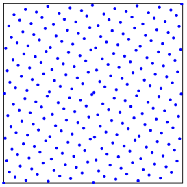
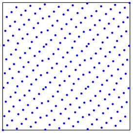
Figure 10: Two-dimensional Hammersley point sets: $\mathcal{H}_{2,8}$ in base $b=2$ with $2^{8}=256$ points (left) and $\mathcal{H}_{3,5}$ in base $b=3$ with $3^{5}=243$ points (right).

Now we need a definition of the local discrepancy in dimension 2. For short, for a two-dimensional point set $\mathcal{P}=\{\boldsymbol{x}_{0},\ldots,\boldsymbol{x}_{N-1}\}$ of $N$ points in $[0,1)^{2}$ we define the local discrepancy (i.e., the deviation from ideal distribution) as

$$\Delta_{\mathcal{P}}(x,y):=\frac{A([0,x)\times[0,y);\mathcal{P})}{N}-xy,$$

where $A([0,x)\times[0,y);\mathcal{P}):=\#\{n\in\{0,1,\ldots,N-1\}\ :\ \boldsymbol{x}_{n}\in[0,x)\times[0,y)\}$.

The link between the local discrepancies of Hammersley point sets (in dimension 2) and van der Corput sequences (in dimension 1) is almost trivial and has already been used in Section 2.4. We state it again in a lemma as it is the fundamental key that permits transferring results for van der Corput sequences to results for Hammersley point sets [44, Lemma 3] .

Lemma 6

Let $m,N$, and $\lambda$ be positive integers with $1\leq N\leq b^{m}$ and $1\leq\lambda<b^{m}$. Then,

$$\Delta_{\mathcal{H}_{b,m}^{\boldsymbol{\sigma}}}\left(\frac{\lambda}{b^{m}},\frac{N}{b^{m}}\right)=\Delta_{Y_{b}^{\Sigma},N}\left(\frac{\lambda}{b^{m}}\right).$$

• The proof is almost immediate: from the definition of $\mathcal{H}_{b,m}^{\boldsymbol{\sigma}}$ the counting functions $A(\tfrac{\lambda}{b^{m}},\tfrac{N}{b^{m}},\mathcal{H}_{b,m}^{\boldsymbol{\sigma}})$ and $A(\tfrac{\lambda}{b^{m}},N,Y_{b}^{\Sigma})$ attain the same value, and on the other hand we have $b^{m}\tfrac{\lambda}{b^{m}}\tfrac{N}{b^{m}}=N\tfrac{\lambda}{b^{m}}$ (note that $\#\mathcal{H}_{b,m}^{\boldsymbol{\sigma}}=b^{m}$), so that the local discrepancies are equal. $\hfill\Box$

From Lemmas 2 and 6, it is possible to obtain (see [44] for the details) the following result.

Theorem 40 (Faure)

For any $m\in\mathbb{N}$ and any $\boldsymbol{\sigma}=(\sigma_{0},\ldots,\sigma_{m-1})\in\mathfrak{S}_{b}^{m}$ we have, with some $c_{m}\in[0,2]$,

$$b^{m}D_{b^{m}}^{*}(\mathcal{H}_{b,m}^{\boldsymbol{\sigma}})=\max\left(\max_{1\leq N\leq b^{m}}\sum_{j=1}^{m}\psi_{b}^{\sigma_{j-1},+}\bigg{(}\frac{N}{b^{j}}\bigg{)}\ ,\ \max_{1\leq N\leq b^{m}}\sum_{j=1}^{m}\psi_{b}^{\sigma_{j-1},-}\bigg{(}\frac{N}{b^{j}}\bigg{)}\right)+c_{m}.$$

Corollary 7

For any $m\in\mathbb{N}$ and any $\boldsymbol{\sigma}=(\sigma_{0},\ldots,\sigma_{m-1})\in\mathfrak{S}_{b}^{m}$ we have, with some $c_{m}\in[-2,2]$,

$$D_{b^{m}}^{*}(\mathcal{H}_{b,m}^{\boldsymbol{\sigma}})\leq D_{b^{m}}^{*}(\mathcal{H}_{b,m})+\frac{c_{m}}{b^{m}}.$$

For the star discrepancy of the classical Hammersley point set in dimension 2 we have the following sharp result according to De Clerck [18] (see also [66] and [92] for the case $b=2$):

Theorem 41 (De Clerck)

For $m\geq 2$ we have:

• if $m\geq 2$ is odd, then

  $$b^{m}D_{b^{m}}^{*}(\mathcal{H}_{b,m})=m\frac{b-1}{4}+\left(\frac{5}{4}+\frac{1}{b}\right)-\frac{1}{4b^{m}};$$

• if $m\geq 2$ is even, then

  $$b^{m}D_{b^{m}}^{*}(\mathcal{H}_{b,m})=m\frac{b^{2}}{4(b+1)}+\left(\frac{5}{4}+\frac{2b+3}{4(b+1)^{2}}\right)-\frac{1}{4b^{m}}\left(1+\frac{2b+3}{(b+1)^{2}}\right).$$

Note that $m=(\log b^{m})/\log b$ and $b^{m}=\#\mathcal{H}_{b,m}$. Hence De Clerck’s result (together with Corollary 7) shows that the star discrepancy of the two-dimensional (generalized) Hammersley point set is of order $D_{b^{m}}^{*}(\mathcal{H}_{b,m})=O((\log b^{m})/b^{m})=O((\log N)/N)$, which is optimal with respect to the order of magnitude in $N=b^{m}$ according to W.M. Schmidt’s general lower bound on the star discrepancy of two-dimensional point sets (cf. Remark 1). We mention that De Clerck [18] also provides the “bad” intervals for which the star discrepancy is attained. Further results for the star discrepancy of generalized Hammersley point sets can be found in [43, 79, 80]. The permutations $\boldsymbol{\sigma}$ can help to minimize the constant which is associated to the leading term $m$ in the star discrepancy formulas, see [44] where several results are obtained with the help of the swapping permutation $\tau_{b}$ applied in various situations, getting analogs in arbitrary bases of results from [79, 80] in base 2.

For the $L_{p}$-discrepancies the situation is quite different. We have:

Theorem 42 (Faure and Pillichshammer)

For any integer base $b\geq 2$ and any $m\in\mathbb{N}_{0}$ we have

$$b^{m}L_{1,b^{m}}(\mathcal{H}_{b,m})=m\frac{b^{2}-1}{12b}+\frac{1}{2}+\frac{1}{4b^{m}}$$

and

$$(b^{m}L_{2,b^{m}}(\mathcal{H}_{b,m}))^{2} = m^{2}\left(\frac{b^{2}-1}{12b}\right)^{2}+m\left(\frac{3b^{4}+10b^{2}-13}{720b^{2}}+\frac{b^{2}-1}{12b}\left(1-\frac{1}{2b^{m}}\right)\right)$$

$$+\frac{3}{8}+\frac{1}{4b^{m}}-\frac{1}{72b^{2m}}.$$

Furthermore, for arbitrary $p\in[1,\infty)$ we have

$$(b^{m}L_{p,b^{m}}(\mathcal{H}_{b,m}))^{p}=m^{p}\left(\frac{b^{2}-1}{12b}\right)^{p}+O_{p,b}(m^{p-1}),$$

where the constant in the $O$-notation only depends on $p$ and $b$. In particular,

$$\lim_{m\rightarrow\infty}\frac{b^{m}L_{p,b^{m}}(\mathcal{H}_{b,m})}{\log b^{m}}=\frac{b^{2}-1}{12b\log b}.$$

A proof of this result can be found in [52]. Theorem 42 implies that the $L_{p}$-discrepancy for finite $p$ is not of optimal order according to the lower bounds of Halász, Roth, and Schmidt for arbitrary $N$-element point sets (which is $L_{p,N}(\mathcal{P})\gg\sqrt{\log N}/N$ in dimension 2, cf. Remark 1). This defect of the classical Hammersley point sets can be overcome when we consider generalized Hammersley point sets. There are various papers which provide sequences of permutations which lead to the optimal order of $L_{2}$-discrepancy (see, for example, [52, 53, 54, 55, 56, 57, 66, 83, 144]). We provide an exemplary result from [52].

Theorem 43 (Faure and Pillichshammer)

Let $\boldsymbol{\sigma}\in\{{\rm id},\tau_{b}\}^{m}$, where $\tau_{b}(k):=b-k-1$ for $k\in\mathbb{Z}_{b}$, and let $l(m)$ denote the number of components of $\boldsymbol{\sigma}$ which are equal to ${\rm id}$. Then we have

$$(b^{m}L_{2,b^{m}}(\mathcal{H}_{b,m}^{\boldsymbol{\sigma}}))^{2} = \displaystyle\left(\frac{b^{2}-1}{12b}\right)^{2}((m-2l(m))^{2}-m)+\frac{b^{2}-1}{12b}\left(1-\frac{1}{2b^{m}}\right)(2l(m)-m)$$

$$+m\frac{b^{4}-1}{90b^{2}}+\frac{3}{8}+\frac{1}{4b^{m}}-\frac{1}{72b^{2m}}.$$

In particular, the $L_{2}$-discrepancy of $\mathcal{H}_{b,m}^{\boldsymbol{\sigma}}$ becomes minimal if we choose a sequence of permutations $\boldsymbol{\sigma}$ in which exactly

$$l_{\min}(m):=\left\{\begin{array}[]{ll}m/2-2&\mbox{ if }b=2,\\ m/2-1&\mbox{ if }3\leq b\leq 6,\\ m/2&\mbox{ if }b\geq 7,\end{array}\right.$$

elements are the identity in the case of even $m$, and

$$l_{\min}(m):=\left\{\begin{array}[]{ll}(m-3)/2&\mbox{ if }2\leq b\leq 3,\\ (m-1)/2&\mbox{ if }b\geq 4,\end{array}\right.$$

elements are the identity in the case of odd $m$. In any case we have

$$\min_{\boldsymbol{\sigma}\in\{{\rm id},\tau_{b}\}^{m}}(b^{m}L_{2,b^{m}}(\mathcal{H}_{b,m}^{\boldsymbol{\sigma}}))^{2}=m\frac{(b^{2}-1)(3b^{2}+13)}{720b^{2}}+O(1).$$ (29)

A generalization of these results and a detailed discussion can be found in [57]. Equation (29) shows that the optimal permutations lead to an $L_{2}$-discrepancy of order $O(\sqrt{m}/b^{m})=O(\sqrt{\log N}/N)$ where $N=b^{m}$ and this is optimal according to the general lower bound of Roth [125]. It is interesting that the minimal $L_{2}$-discrepancy only depends on the number of ${\rm id}$-permutations and not on their position within $\boldsymbol{\sigma}$. Not quite exact as the result for $L_{2,N}$, but with the same essence, is the next result for the $L_{p}$-discrepancy (with $p\in[1,\infty)$) of $\mathcal{H}_{2,m}^{\boldsymbol{\sigma}}$.

Theorem 44 (Markhasin)

Let $p\in[1,\infty)$. Let $\boldsymbol{\sigma}\in\{{\rm id},\tau_{2}\}^{m}$ and let $l(m)$ be the number of components of $\boldsymbol{\sigma}$ which are equal to ${\rm id}$. Then we have

$$L_{p,2^{m}}(\mathcal{H}_{2,m}^{\boldsymbol{\sigma}})\ll_{p}\frac{\sqrt{m}}{2^{m}}\ll\frac{\sqrt{\log N}}{N}\ \ \ \mbox{ where $N=2^{m}$}$$

if and only if $|2l(m)-m|\ll_{p}\sqrt{m}$.

The proof of this result according to Markhasin [99, 100] is indirect via optimality of the norm of the discrepancy function in Besov spaces with dominating mixed smoothness together with embedding theorems between Besov spaces and Triebel-Lizorkin spaces which contain $L_{p}$-spaces as special cases. The main tool there is the computation of Haar coefficients of the discrepancy function, which, for the generalized Hammersley point sets, were already computed in [71]. A direct proof of Theorem 44 via Littlewood-Paley theory, which is accessible without knowledge of function space theory, can be found in [72]. Although Theorem 44 was proved only in base $b=2$ a similar result should hold for general bases $b$. This is work in progress.

We close this section by mentioning that besides permutations also a symmetrization of the classical Hammersley point set leads to the optimal order of $L_{p}$-discrepancy with respect to the order of magnitude in $N$ (see, e.g., [72, Theorems 2 and 3]). Furthermore, also geometric shifts of the Hammersley point set and their influence on $L_{2}$-discrepancy were studied by Bilyk [11].

4.2 The Halton sequence

We now come to a very natural extension of van der Corput sequences to arbitrary dimensions $s\in\mathbb{N}$.

The classical Halton sequence.

Let $s\in\mathbb{N}$. A natural generalization of the one-dimensional van der Corput sequence to dimension $s$ is to choose $s$ different bases $b_{1},b_{2},\ldots,b_{s}\geq 2$ and to concatenate component-wise the van der Corput sequences with bases $b_{1},b_{2},\ldots,b_{s}$, respectively, to a sequence in the $s$-dimensional unit cube. Such a sequence is called a Halton sequence.

Definition 12

Let $s\geq 1$ and let $\boldsymbol{b}=(b_{1},b_{2},\ldots,b_{s})$ be a vector of integers greater than 1. The $s$-dimensional Halton sequence in bases $b_{1},b_{2},\ldots,b_{s}$ is given as $H_{\boldsymbol{b}}=(\boldsymbol{y}_{n})_{n\geq 0}$ where

$$\boldsymbol{y}_{n}=(Y_{b_{1}}(n),Y_{b_{2}}(n),\ldots,Y_{b_{s}}(n))\ \ \ \mbox{ for $n\in\mathbb{N}_{0}$.}$$

A minimal requirement on the Halton sequence is that it should be uniformly distributed modulo 1. This depends on the choice of the bases $b_{1},b_{2},\ldots,b_{s}$, as can be seen in the following theorem.

Theorem 45

The Halton sequence $H_{\boldsymbol{b}}$ is uniformly distributed modulo 1 if and only if $b_{1},b_{2},\ldots,b_{s}$ are pairwise coprime.

The result in Theorem 45 follows by similar arguments as used in the proof of uniform distribution modulo 1 of the van der Corput sequence together with the Chinese Remainder Theorem.

From now on we assume that $\boldsymbol{b}$ is a vector of pairwise coprime integers. In this case the Halton sequence even has a low discrepancy of order of magnitude $O((\log N)^{s}/N)$. This was first shown by Halton [65]. The following result is due to Niederreiter [106] and can be shown by a tricky induction argument. Further discrepancy estimates for the Halton sequence can be found in [24, 31, 76, 96, 103].

Theorem 46 (Niederreiter)

If $H_{\boldsymbol{b}}$ is the Halton sequence in pairwise coprime bases $b_{1},b_{2},\ldots,b_{s}$, then

$$D_{N}^{*}(H_{\boldsymbol{b}})<\frac{s}{N}+\frac{1}{N}\prod_{j=1}^{s}\left(\frac{b_{j}-1}{2\log b_{j}}\log N+\frac{b_{j}+1}{2}\right)\ \ \ \mbox{ for all }\ N\in\mathbb{N}.$$

It was a long standing open question if the discrepancy estimate for Halton sequences is best possible with respect to the order of magnitude in $N$. Until recently one only had the general lower bound due to Kuipers and Niederreiter [85] (which is based on the result of Roth [125] for finite point sets) which states that there exists some $c_{s}>0$ such that for every sequence $X$ in $[0,1)^{s}$ we have

$$D_{N}^{*}(X)\geq c_{s}\frac{(\log N)^{s/2}}{N}\ \ \ \mbox{ for infinitely many $N\in\mathbb{N}$}.$$ (30)

We add that there is a slight but remarkable improvement of the exponent of the $\log N$-term. It follows from a result of Bilyk, Lacey, and Vagharshakyan [13] for finite point sets that there exists some $c_{s}>0$ and $\eta_{s}\in(0,\tfrac{1}{2})$ such that for every sequence $X$ in $[0,1)^{s}$ we have

$$D_{N}^{*}(X)\geq c_{s}\frac{(\log N)^{s/2+\eta_{s}}}{N}\ \ \ \mbox{for infinitely many $N\in\mathbb{N}$.}$$ (31)

For $s\geq 2$ the sharp lower bound for the star discrepancy of infinite sequences is still unknown. It is conjectured that it is significantly larger than the one given in (31). In general, finding a sharp lower bound seems to be a very difficult problem. We also refer to [12] for a discussion of these questions.

In 2015 Levin [98] obtained a solution of this question for the important sub-class of Halton sequences. He could show that the existing upper bounds on the star discrepancy of the Halton sequence are optimal with respect to the order of magnitude in $N$.

Theorem 47 (Levin)

Let $s\geq 2$ and let $B:=b_{1}b_{2}\cdots b_{s}$ and $m_{0}=\lfloor 2B\log_{2}b_{0}\rfloor+2$. Then

$$\sup_{1\leq N\leq 2^{mm_{0}}}ND_{N}^{*}(H_{\boldsymbol{b}})\geq\frac{m^{s}}{8B}\ \ \ \mbox{ for all $m\geq B$.}$$

In particular, there exists some $c_{\boldsymbol{b},s}>0$ such that

$$D_{N}^{*}(H_{\boldsymbol{b}})\geq c_{\boldsymbol{b},s}\frac{(\log N)^{s}}{N}\ \ \ \mbox{ for infinitely many $N\in\mathbb{N}$.}$$

Atanassov’s results.

The bound in Theorem 46 has a slightly defective appearance when one considers the constant in the leading $\log N$-term. Consider the quantity

$$d_{s}^{\ast}(X):=\limsup_{N\rightarrow\infty}\frac{ND_{N}^{*}(X)}{(\log N)^{s}}$$ (32)

for Halton sequences $X=H_{\boldsymbol{b}}$. From Theorem 46 it follows that

$$d_{s}^{\ast}(H_{\boldsymbol{b}})\leq\prod_{j=1}^{s}\frac{b_{j}-1}{2\log b_{j}}=:c_{s}.$$

This bound $c_{s}$ is large and grows very fast to infinity for growing dimensions $s$. For example, if $b_{1},\ldots,b_{s}$ are the first $s$ prime numbers, then the Prime Number Theorem implies that $b_{j}\approx j\log j$ for large $j$ and hence

$$c_{s}=\prod_{j=1}^{s}\frac{b_{j}-1}{2\log b_{j}}\approx\prod_{j=1}^{s}\frac{j\log j}{2\log(j\log j)}\approx\prod_{j=1}^{s}\frac{j\log j}{2\log j}=\frac{s!}{2^{s}}.$$

Also the bounds from [31, 76, 96, 103] have the same disadvantage. In 2004, Atanassov [2] was able to overcome this particular disadvantage (see also the recent survey [45], where Atanassov’s method is outlined).

Theorem 48 (Atanassov)

If $H_{\boldsymbol{b}}$ is the Halton sequence in pairwise coprime bases $b_{1},b_{2},\ldots,b_{s}$, then

$$D_{N}^{\ast}(H_{\boldsymbol{b}})\leq\left[\frac{1}{s!}\prod_{j=1}^{s}\left(\frac{\lfloor b_{j}/2\rfloor\log N}{\log b_{j}}+s\right)+\sum_{k=0}^{s-1}\frac{b_{k+1}}{k!}\prod_{j=1}^{k}\left(\frac{\lfloor b_{j}/2\rfloor\log N}{\log b_{j}}+k\right)\right]\frac{1}{N}.$$

This result implies that

$$d_{s}^{\ast}(H_{\boldsymbol{b}})\leq\frac{1}{s!}\prod_{j=1}^{s}\frac{\lfloor b_{j}/2\rfloor}{\log b_{j}}.$$

If again $b_{1},\ldots,b_{s}$ are the first $s$ prime numbers, then this implies that $d_{s}^{\ast}(H_{\boldsymbol{b}})\ll\frac{1}{2^{s}s}$ and hence $d_{s}^{\ast}(H_{\boldsymbol{b}})$ tends to zero at an exponential rate as $s\rightarrow\infty$. More exact, we have

$$\limsup_{s\rightarrow\infty}\frac{\log d_{s}^{*}(H_{\boldsymbol{b}})}{s}\leq-\log 2.$$ (33)

Generalized Halton sequences.

A disadvantage of the classical Halton sequence is that there seem to exist quite many correlations between the components from the higher dimensions, see e.g. [94, 96]. To overcome this problem one often studies generalized Halton sequences $H_{\boldsymbol{b}}^{\Sigma_{1},\ldots,\Sigma_{s}}$ which are given by $\boldsymbol{y}_{n}=(Y_{b_{1}}^{\Sigma_{1}}(n),Y_{b_{2}}^{\Sigma_{2}}(n),\ldots,Y_{b_{s}}^{\Sigma_{s}}(n))$ for $n\in\mathbb{N}_{0}$, where $\Sigma_{j}=(\sigma_{j,r})_{r\geq 0}$ are sequences of permutations of $\{0,1,\ldots,b_{j}\}$ for $1\leq j\leq s$; see again [94] and the references therein. The discrepancy estimate from Theorem 48 remains valid also for generalized Halton sequences. However, it is important to note that the permutations can even lead to a drastic reduction of the star discrepancy of $H_{\boldsymbol{b}}$. For example, in [2] Atanassov constructed specific sequences of permutations $\Sigma_{1},\ldots,\Sigma_{s}$ which lead to exactly such a result:

Let $b_{1},\ldots,b_{s}$ be distinct prime numbers. Then integers $k_{1},\ldots,k_{s}$ are called “admissible” to these primes, if $b_{j}\nmid k_{j}$ for $1\leq j\leq s$ and if for each set of integers $a_{1},\ldots,a_{s}$ with $b_{j}\nmid a_{j}$ for $1\leq j\leq s$, there exist integers $\alpha_{1},\ldots,\alpha_{s}$ such that

$$k_{j}^{\alpha_{j}}\prod_{i=1\atop i\not=j}^{s}b_{i}^{\alpha_{i}}\equiv a_{j}\pmod{b_{j}}\ \ \ \mbox{ for all $1\leq j\leq s$.}$$

Now let $b_{1},\ldots,b_{s}$ be distinct prime numbers and let $k_{1},\ldots,k_{s}$ be “admissible” to these primes. For each $j\in\{1,\ldots,s\}$ define a sequence of permutations $\Sigma_{j}=(\tau_{j,r})_{r\geq 0}$ of $\mathbb{Z}_{b_{j}}$ by $\tau_{j,r}(x):=xk_{j}^{r}\pmod{b_{j}}$. For these so-called scramblings we have ([2, Theorem 2.3])

Theorem 49 (Atanassov)

Let $b_{1},\ldots,b_{s}$ be distinct prime numbers and let $k_{1},\ldots,k_{s}$ be “admissible” to these primes. For the sequences of permutations constructed above we have

$$D_{N}^{*}(H_{\boldsymbol{b}}^{\Sigma_{1},\ldots,\Sigma_{s}})\leq\left(\frac{1}{s!}\sum_{j=1}^{s}\log b_{j}\right)\left(\prod_{i=1}^{s}\frac{b_{i}(1+\log b_{i})}{(b_{i}-1)\log b_{i}}\right)\frac{(\log N)^{s}}{N}+O\left(\frac{(\log N)^{s-1}}{N}\right).$$

From this discrepancy bound it follows easily (see, for example, [48]) that

$$\limsup_{s\rightarrow\infty}\frac{\log d_{s}^{*}(H_{\boldsymbol{b}}^{\Sigma_{1},\ldots,\Sigma_{s}})}{s\log s}=-1,$$ (34)

and this is a drastic improvement compared to (33), since now $d_{s}^{*}(H_{\boldsymbol{b}}^{\Sigma_{1},\ldots,\Sigma_{s}})$ tends to zero at a superexponential rate as $s\rightarrow\infty$.

Randomized and deterministic scrambled Halton sequences.

Another possibility to overcome the problem of correlations between the components from the higher dimensions of Halton sequences is to use so-called “random-start” Halton sequences which are based on generalizing the Halton sequence in terms of von Neumann-Kakutani transformations, i.e., the sequence $((T_{b_{1}}^{n}x_{1},T_{b_{2}}^{n}x_{2},\ldots,T_{b_{s}}^{n}x_{s}))_{n\geq 0}$ with $(x_{1},x_{2},\ldots,x_{s})\in[0,1)^{s}$; see [111, 135, 142].

One could also consider linear digit scramblings: Various types of linear digit scramblings as introduced at the end of Section 3.2 have been used by many authors with the aim to improve the behavior of Halton sequences for multi-dimensional integration based on quasi-Monte Carlo methods (note that also Atanassov’s permutations $\tau_{j,r}$ introduced above are specific examples of linear digit scramblings). An extensive comparative study of such methods is given in [48] where a new effective way of scrambling is also proposed. This method consists of the search for a list of good multipliers by means of the diaphony of one-dimensional projections of Halton sequences, coupled with a criterion based on two-dimensional projections that selects the best multipliers in the preceding list (the diaphony is considered, rather than the discrepancy, because it is easier and faster to compute, see [41] for more details). Several numerical experiments show a regular and better behavior of these multipliers in comparison with other ones (including multipliers from the modified Halton sequences of Atanassov). The study also compares linear digit scramblings with “random-start” Halton sequences and suggests that these sequences have almost the same behavior as original Halton sequences.

Further remarks.

Bounded remainder intervals for Halton sequences are well understood and it is known that they are of the form $[0,a_{1}b_{1}^{-m_{1}})\times\cdots\times[0,a_{s}b_{s}^{-m_{s}})$. We refer to [61, Theorem 70] and the references therein. Subsequences of the Halton sequence are studied in [70, 75, 81]. Ergodic properties of $\beta$-adic Halton sequences are studied in [74].

Also the polynomial version of the van der Corput sequence as presented in Section 3.4 can be generalized to polynomial Halton sequences which are a special sub-class of $(t,s)$-sequences then; see [137].

The Hammersley point set.

A finite version of the Halton sequence in dimension $s-1$ is the Hammersley point set in dimension $s$ (cf. Definition 11 for $s=2$).

Definition 13 (Hammersley point set)

Let $s,N\in\mathbb{N}$, $s\geq 2$, and let $\boldsymbol{b}=(b_{1},b_{2},\ldots,b_{s-1})$ be a vector of integers with $b_{j}\geq 2$. The $s$-dimensional Hammersley point set in bases $b_{1},b_{2},\ldots,b_{s-1}$ is given as $\mathcal{H}_{\boldsymbol{b},N}=\{\boldsymbol{y}_{0},\boldsymbol{y}_{1},\ldots,\boldsymbol{y}_{N-1}\}$ where

$$\boldsymbol{y}_{n}=\left(\frac{n}{N},Y_{b_{1}}(n),Y_{b_{2}}(n),\ldots,Y_{b_{s-1}}(n)\right)\ \ \ \mbox{ for $n=0,1,\ldots,N-1$.}$$

According to a well-known relation between the star discrepancy of infinite sequences in dimension $s-1$ and finite point sets in dimension $s$, whose elements have first coordinate of the form $n/N$ (see, e.g., [24, Lemma 3.45] or [106, Lemma 3.7]) it follows from Theorem 46 that if $b_{1},b_{2},\ldots,b_{s-1}$ are pairwise coprime integers, then

$$D_{N}^{*}(\mathcal{H}_{\boldsymbol{b},N})\ll_{s,\boldsymbol{b}}\frac{(\log N)^{s-1}}{N}.$$

See, e.g., [24, Chapter 3.4] or [106, Chapter 3] for more information in this direction. For generalized Hammersley point sets we refer to [36].

4.3 $(t,s)$-sequences

In Section 4.2 we generalized the van der Corput sequence to arbitrary dimension by choosing different bases, one per coordinate direction, and concatenating component-wise van der Corput sequences in these bases. We now introduce a generalization to arbitrary dimension where the base $b$ is kept fixed for all dimensions.

Definition of $(t,s)$-sequences.

In the one-dimensional case (see Definition 4 in Section 3.2), we defined a $(0,1)$-sequence in base $b$ as a sequence of points such that each elementary interval of a certain size contains exactly one element of the corresponding segment of the sequence. In higher dimensions, the idea of a $(t,s)$-sequence in base $b$ generalizes this concept. However, the condition that then higher-dimensional elementary intervals all contain exactly one point of the segments of the sequence is, for combinatorial reasons, no longer sustainable in general. Therefore, one needs additional parameters to specify how many points lie in the elementary intervals. To be more precise, we have the following definition that generalizes Definition 4. The general idea of this definition is due to Niederreiter [104], but there also were earlier definitions of a similar flavor for special cases by Sobol’ [132] and Faure [33].

Definition 14

Let $b\geq 2$, $t\geq 0$, and $s\geq 1$ be integers. A sequence $(\boldsymbol{x}_{n})_{n\geq 0}$ in $[0,1)^{s}$ is called a $(t,s)$-sequence in base $b$ (in the broad sense) if for all $l,m\in\mathbb{N}_{0}$ with $m\geq t$, every elementary interval of volume $b^{t-m}$ of the form

$$\left[\frac{a_{1}}{b^{d_{1}}},\frac{a_{1}+1}{b^{d_{1}}}\right)\times\cdots\times\left[\frac{a_{s}}{b^{d_{s}}},\frac{a_{s}+1}{b^{d_{s}}}\right),$$

with $a_{j},d_{j}\in\mathbb{N}_{0}$ such that $0\leq a_{j}<b^{d_{j}}$ for $1\leq j\leq s$, contains exactly $b^{t}$ elements of the point set

$$\{[\boldsymbol{x}_{n}]_{b,m}:\ lb^{m}\leq n\leq(l+1)b^{m}-1\}\ \ \ \mbox{ for all $l\in\mathbb{N}_{0}$.}$$

Here the truncation operator $[\cdot]_{b,m}$ is applied component-wise.

Some remarks on this definition are in order:

Remark 8

• The original definition of $(t,s)$-sequences in base $b$ due to Niederreiter [104, 106] is the same but with $[\boldsymbol{x}_{n}]_{b,m}$ replaced by $\boldsymbol{x}_{n}$. The definition presented here goes back to Niederreiter and Xing (see, e.g., [108, Chapter 8]).

• It is well known that every $(t,s)$-sequence in base $b$ is uniformly distributed modulo 1 (see, e.g., [24, 96]).

• If one would like to have greater flexibility in the definition of a $(t,s)$-sequence, it is also possible to allow the parameter $t$ to depend on the parameter $m\in\mathbb{N}_{0}$ in the above definition. In this case, the value of $t$ can vary with $m$, and instead of a $(t,s)$-sequence, one then has a $({\bf T},s)$-sequence with ${\bf T}=(t(m))_{m\geq 0}$. For the sake of simplicity, we concentrate on discussing only $(t,s)$-sequences with a fixed $t$ in the present paper. For further information on $({\bf T},s)$-sequences, we refer the interested reader to [90] and [24, Chapters 4 and 5].

• Note that in Definition 14 lower values of $t$ mean better distribution properties, with $t=0$ being the optimal case. For this reason $t$ is called the quality parameter of the sequence. For the one-dimensional sequences presented in Section 3.2, a value of $t=0$ can be reached, however for general sequences in $[0,1)^{s}$ this is not always achievable. For instance, a $(0,s)$-sequence in base $b$ can only exist if $s\leq b$ (if $b$ is a prime power, then the “only if” can be replaced by “if and only if”). The question which $t$ for which parameter configuration $(s,b)$ is optimal has gained much interest. In [107] it was shown that for the minimal achievable $t$ we have

  $$t\geq\frac{s}{b}-\log_{b}\left(\frac{(b-1)s+b+1}{2}\right),$$

  where $\log_{b}$ is the logarithm to the base $b$. For further information in this direction we also refer to [131].

As it was the case for $(0,1)$-sequences, also for $(t,s)$-sequences in base $b$ there exists a digital version generated by $\mathbb{N}\times\mathbb{N}$ matrices over a finite ring $R$. As in the one-dimensional case we restrict ourselves to the case where $b$ is a prime power and $R$ is the finite field $\mathbb{F}_{b}$ of order $b$. Indeed, $s$-dimensional digital sequences over $\mathbb{F}_{b}$ are obtained by choosing, for each $j\in\{1,\ldots,s\}$, an $\mathbb{N}\times\mathbb{N}$ matrix $C^{(j)}=(c_{r,k}^{(j)})_{r,k\geq 0}$ over $\mathbb{F}_{b}$. Using the construction method outlined in Definition 5, one obtains a sequence $X_{b}^{C^{(j)}}=(x_{n}^{(j)})_{n\geq 0}$ for each $j\in\{1,\ldots,s\}$. The $s$-dimensional sequence then consists of the points

$$\boldsymbol{x}_{n}:=(x_{n}^{(1)},\ldots,x_{n}^{(s)})\ \ \ \ \mbox{ for $n\in\mathbb{N}_{0}$.}$$ (35)

The sequence $(\boldsymbol{x}_{n})_{n\geq 0}$ is often called a digital sequence over $\mathbb{F}_{b}$.

The matrices $C^{(j)}$ also determine the $t$-value of the corresponding digital sequence. Indeed, let $C^{(j)}(m\times m)$ be the left upper $m\times m$ submatrix of $C^{(j)}$. If there exists a $t\in\mathbb{N}_{0}$ such that for every choice of nonnegative integers $m>t$ and $d_{1},\ldots,d_{s}\in\mathbb{N}_{0}$ with $d_{1}+\cdots+d_{s}=m-t$,

• the first $d_{1}$ rows of $C^{(1)}(m\times m)$, together with

• the first $d_{2}$ rows of $C^{(2)}(m\times m)$, together with

• etc., up to
  

• the first $d_{s}$ rows of $C^{(s)}(m\times m)$,

(these are $m-t$ vectors in $\mathbb{F}_{b}^{m}$) is a linearly independent set over $\mathbb{F}_{b}$, then the digital sequence (35) is a $(t,s)$-sequence in base $b$ which is then called a digital $(t,s)$-sequence over $\mathbb{F}_{b}$ (see [24, 96, 104, 106]). Hence, finding a $(t,s)$-sequence in base $b$ with a low value of $t$ boils down to the problem of finding generating matrices $C^{(1)},\ldots,C^{(s)}$ whose row vectors satisfy the necessary linear independence conditions.

The dynamics behind digital $(t,s)$-sequences was studied by Grabner, Hellekalek, and Liardet. We do not go into details here and just refer to the papers [61] and [69].

Generalized Niederreiter sequences.

A particular kind of digital $(t,s)$-sequences are so-called Niederreiter sequences, whose points are constructed by means of polynomials over finite fields. These sequences offer an explicit way of constructing the generating matrices of powerful digital $(t,s)$-sequences over $\mathbb{F}_{b}$. They were introduced in [105], and their definition was further extended to generalized Niederreiter sequences by Tezuka in [138]. Following the presentation in [24], a generalized Niederreiter sequence is obtained as follows.

Let $s\in\mathbb{N}$, let $b$ be a prime power, and let $p_{1},\ldots,p_{s}$ be distinct monic irreducible polynomials over $\mathbb{F}_{b}$. Let $e_{j}:=\deg(p_{j})$ for $1\leq j\leq s$. Moreover, choose polynomials $y_{j,i,k}$ for $1\leq j\leq s$, $i\geq 1$, and $0\leq k<e_{j}$ with the property that the set $\{y_{j,i,k}:0\leq k<e_{j}\}$ is linearly independent modulo $p_{j}$ over $\mathbb{F}_{b}$. Then consider the expansions

$$\frac{y_{j,i,k}(x)}{p_{j}(x)^{i}}=\sum_{r=0}^{\infty}a^{(j)}(i,k,r)x^{-r-1}$$

over the field $\mathbb{F}_{b}((x^{-1}))$ for $1\leq j\leq s$, $i\geq 1$, and $0\leq k<e_{j}$. We use these expansions to define the generating matrices of a digital sequence; for $1\leq j\leq s$ let $C^{(j)}=(c_{i,r}^{(j)})_{i\geq 1,r\geq 0}$ be given by

$$c_{i,r}^{(j)}=a^{(j)}(Q+1,k,r)\in\mathbb{F}_{b}$$ (36)

for $1\leq j\leq s$, $i\geq 1$, and $0\leq k<e_{j}$, where $i-1=Qe_{j}+k$ with suitable integers $Q=Q(j,i)$ and $k=k(j,i)$ with $0\leq k<e_{j}$.

Definition 15

A digital sequence over $\mathbb{F}_{b}$ generated by $C^{(1)},\ldots,C^{(s)}$ as given by (36) is called generalized Niederreiter sequence.

Every generalized Niederreiter sequence is a digital $(t,s)$-sequence over $\mathbb{F}_{b}$ with

$$t=\sum_{j=1}^{s}(e_{j}-1),$$

see, e.g., [24, 96, 106].

The concept of generalized Niederreiter sequences comprises earlier constructions due to Sobol’ [132], Faure [33], and Niederreiter [105], which are nowadays very popular as underlying sample points for quasi-Monte Carlo integration rules (cf. [24, 106]).

• A Sobol’ sequence is the generalized Niederreiter sequence where $b=2$, $p_{1}(x)=x$, and, for $j=2,\ldots,s$, $p_{j}(x)$ is the $(j-1)$-st primitive polynomial in a sequence of all primitive polynomials over $\mathbb{F}_{2}$ arranged according to nondecreasing degrees. Further, there are polynomials $g_{j,0},\ldots,g_{j,e_{j}-1}$ with $\deg(g_{j,h})=e_{j}-h+1$ such that $y_{j,i,k}=g_{j,k}$ for all $i\in\mathbb{N}$, $k\in\{0,\ldots,e_{j}-1\}$, and $j\in\{1,\ldots,s\}$, see [138, Remark 2].

• A Faure sequence corresponds to the case where the base $b$ is a prime number such that $b\geq s$, $p_{j}(x)=x-j+1$ for $j=1,2,\ldots,s$, and all $y_{i,j,k}\equiv 1$, see [138, Remark 3]. In particular, every Faure sequence is a $(0,s)$-sequence. The matrices of a Faure sequence can be given explicitly; there exist $s$ pairwise different elements of $\mathbb{F}_{b}$, $\beta_{1},\ldots,\beta_{s}$, which are determined by the choice of the $p_{j}$ such that the $i$th matrix is given as

  $$C_{i}:=\left(\begin{array}[]{cccccc}1&{1\choose 0}\beta_{i}^{1}&{2\choose 0}\beta_{i}^{2}&{3\choose 0}\beta_{i}^{3}&{4\choose 0}\beta_{i}^{4}&\ldots\\ \\ 0&1&{2\choose 1}\beta_{i}^{1}&{3\choose 1}\beta_{i}^{2}&{4\choose 1}\beta_{i}^{3}&\ldots\\ \\ 0&0&1&{3\choose 2}\beta_{i}^{1}&{4\choose 2}\beta_{i}^{2}&\ldots\\ \\ \vdots&\ddots&\ddots&1&{4\choose 3}\beta_{i}^{1}&\ldots\\ \\ \vdots&\ddots&\ddots&\ddots&\ddots&\ddots\end{array}\right)\in\mathbb{F}_{b}^{\mathbb{N}\times\mathbb{N}},$$

  where the binomial coefficients have to be taken modulo $b$.

• A Niederreiter sequence corresponds to the case where $b$ is a prime power and the $y_{j,i,k}$ are of the form $y_{j,i,k}(x)=x^{k}g_{j,i}(x)$ with polynomials $g_{j,i}\in\mathbb{F}_{b}[x]$ such that $\gcd(g_{j,i},p_{j})=1$, see [138, Remark 4].

The currently best constructions for digital sequences with respect to the quality parameter $t$ are based on methods from algebraic geometry. These constructions were developed in a series of papers by Niederreiter and Xing. For an introduction to this subject and an overview we refer to the book by Niederreiter and Xing [108, Chapter 8]. A survey can also be found in the book [24, Chapter 8].

Linear digit scramblings have also been used to improve the quality of $(0,s)$-sequences for quasi-Monte Carlo methods, with the same approach as for Halton sequences in Section 4.2, see [95].

The star discrepancy of $(t,s)$-sequences.

Regarding the discrepancy of $(t,s)$-sequences, it is, not surprisingly, more difficult than in the one-dimensional case to come up with good discrepancy bounds. Let us start with discussing the star discrepancy, for which there has been much progress over the past years. Regarding lower discrepancy bounds, the best results for dimensions $s\geq 2$ are the general bounds (30) and (31), excepted in the special case of the two-dimensional $(0,2)$-sequence of Sobol’ (also a Faure sequence), say $S_{2}$, obtained with the van der Corput sequence $Y_{2}$ on the $x$-axis and its image by the Pascal matrix modulo 2 on the $y$-axis. For this sequence, Faure and Chaix [46] were able to obtain the exact order $(\log N)^{2}$ for $ND^{*}_{N}(S_{2})$ with a tight lower bound. Together with an upper bound from Pillichshammer in [116], we have the following estimate:

Theorem 50 (Faure and Chaix, Pillichshammer)

The sequence $S_{2}$ satisfies the inequalities

$$\frac{1}{24(\log 2)^{2}}\leq\limsup_{N\rightarrow\infty}\frac{ND^{*}_{N}(S_{2})}{(\log N)^{2}}\leq\frac{1}{12(\log 2)^{2}}\cdot$$

Until now, this is the only case of a $(t,s)$-sequence in dimension $s\geq 2$ for which the exact order of star discrepancy is known. Based on thorough computations, Faure and Chaix conjectured that the left inequality should be an equality.

However, for any dimension, there is a metric result of Larcher and Pillichshammer [93] for general digital sequences over prime fields.

Theorem 51 (Larcher and Pillichshammer)

Let $s\in\mathbb{N}$ and let $b$ be a prime number. Then for almost all $s$-tuples $(C_{1},\ldots,C_{s})\in(\mathbb{F}_{b}^{\mathbb{N}\times\mathbb{N}})^{s}$ of generating matrices the corresponding digital sequences have a star discrepancy satisfying

$$D_{N}^{\ast}\geq c(b,s)\frac{(\log N)^{s}\log\log N}{N}\ \ \ \mbox{ for infinitely many }N\in\mathbb{N}$$

with some $c(b,s)>0$ not depending on $N$.

The situation is different for upper discrepancy bounds, where one can use the structure of $(t,s)$-sequences to show strong results which are better than the metric lower bound from Theorem 51. Upper bounds for the star discrepancy that hold for arbitrary $(t,s)$-sequences are due to Niederreiter [104], which are based on a clever recursion argument. The bounds in [104] were slightly refined in [78], and in a series of papers [47, 49, 50], further improvements were shown. We shortly summarize some of the most up-to-date results. Star discrepancy bounds for $(t,s)$-sequences can be seen from two different perspectives. One may either try to optimize the term involving the highest power of $\log N$, including the constants, as this yields the asymptotically best discrepancy bounds. On the other hand, one may try to optimize the bounds globally such that for the non-asymptotic setting the bounds might be better than those that are optimized with respect to the leading term.

Regarding the former approach, Faure and Kritzer showed in [47] the currently best general star discrepancy bounds for general $(t,s)$-sequences, where the constant in the leading term is the lowest currently known. The following result was shown in [47] using a recursion on $s$ and a discrepancy bound for finite point sets known as $(t,m,s)$-nets.

Theorem 52 (Faure and Kritzer)

Let $s\geq 2$ and let $S_{s}$ be a $(t,s)$-sequence in base $b$. Then it is true that

$$D_{N}^{\ast}(S_{s})\leq c_{s,b}\,b^{t}\,\frac{(\log N)^{s}}{N}+O\left(b^{t}\,\frac{(\log N)^{s-1}}{N}\right),$$

where

$$c_{s,b}=\begin{cases}\frac{1}{s!}\frac{b^{2}}{2(b^{2}-1)}\left(\frac{b-1}{2\log b}\right)^{s}&\mbox{if $b$ is even,}\\ \frac{1}{s!}\frac{1}{2}\left(\frac{b-1}{2\log b}\right)^{s}&\mbox{if $b$ is odd.}\end{cases}$$

If we consider the quantity $d_{s}^{*}$ as defined in (32) for $(t,s)$-sequences in base $b$, then we obtain from Theorem 52 that

$$d_{s}^{*}(S_{s})\leq c_{s,b}b^{t}.$$

It is known that for any $s,b\in\mathbb{N}$, $b\geq 2$, one can construct a $(t_{b}(s),s)$-sequence $S_{s}^{\ast}$ in base $b$ with $t_{b}(s)\asymp_{b}s$. These constructions are based on the method of Niederreiter and Xing (see [108, Chapter 8]). For such sequences we obtain

$$\limsup_{s\rightarrow\infty}\frac{\log d_{s}^{\ast}(S_{s}^{\ast})}{s\log s}\leq-1$$

and hence $d_{s}^{\ast}(S_{s}^{\ast})$ tends to zero at a superexponential rate as $s\rightarrow\infty$. This is the same rate as for the special generalized Halton sequence given by Atanassov [2], cf. (34) in Section 4.2. Remember that the analog result for Halton sequences given in (33) is much weaker. A comparison is also discussed in [48].

The paper [47] contains also a result where all constants in the star discrepancy bounds for $(t,s)$-sequences are made explicit (cf. [47, Theorem 2]). However, the focus of [47] lies on optimizing the leading constant $c_{s}$. Faure and Lemieux showed in [49, 50] further upper discrepancy bounds which are not optimized regarding $c_{s}$ but which in the non-asymptotic setting (i.e., for smaller values of $N$) yield better discrepancy bounds than [47, Theorem 2]. The bounds of Faure and Lemieux are as follows.

Theorem 53 (Faure and Lemieux)

Let $S_{s}$ be a $(t,s)$-sequence in base $b$. For any $N\in\mathbb{N}$ it is true that

$$D_{N}^{\ast}(S_{s})\leq\frac{b^{t}}{s!}\left(\left\lfloor\frac{b}{2}\right\rfloor\frac{\log N}{\log b}+s\right)^{s}\frac{1}{N}+\frac{b^{t}}{N}\sum_{k=0}^{s-1}\frac{b}{k!}\left(\left\lfloor\frac{b}{2}\right\rfloor\frac{\log N}{\log b}+k\right)^{k}.$$

Theorem 53 was shown in [49] by an adaption of Atanassov’s method for Halton sequences to $(t,s)$-sequences. Finally, in [50, Theorem 1], the following improvement of Theorem 53 was shown.

Theorem 54 (Faure and Lemieux)

Let $S_{s}$ be a $(t,s)$-sequence in base $b$. For any $N\in\mathbb{N}$ it is true that

$$D_{N}^{\ast}(S_{s})\leq\frac{b^{t}}{s!}\left(\frac{b-1}{2}\right)^{s}\frac{1}{N}\prod_{k=1}^{s}\left(\frac{\log N}{\log b}+\gamma_{b}k\right)+\frac{b^{t}}{N}\sum_{k=0}^{s-1}\frac{b}{k!}\left(\frac{b-1}{2}\right)^{k}\prod_{\ell=1}^{k}\left(\frac{\log N}{\log b}+\gamma_{b}\ell\right),$$

where $\gamma_{b}:=2-(b\pmod{2})$.

Numerical experiments in [51] for different values of $N$ and the other parameters show that the bounds in Theorems 53 and 54 may have an advantage over those in Theorem 52 in the non-asymptotic setting.

Finally, we mention that special discrepancy estimates for generalized Niederreiter sequences were recently shown by Tezuka in [139] and then improved for even bases by Faure and Lemieux [50, Theorem 2].

Theorem 55 (Tezuka, Faure, and Lemieux)

Let $S_{s}$ be a generalized Niederreiter sequence in dimension $s$. Then it is true that

$$D_{N}^{\ast}(S_{s}) \leq \frac{1}{s!}\frac{1}{N}\prod_{j=1}^{s}\left(\frac{b^{e_{j}}-1}{2e_{j}}\left(\frac{\log N}{\log b}+\sum_{i=1}^{s}e_{i}\right)+s\right)$$

$$+\frac{1}{N}\sum_{k=0}^{s-1}\frac{b^{e_{k+1}}}{k!}\prod_{i=1}^{k}\left(\frac{b^{e_{i}}-1}{2e_{i}}\left(\frac{\log N}{\log b}+\sum_{r=1}^{s}e_{r}\right)+k\right),$$

where the $e_{j}$, $1\leq j\leq s$, are the degrees of the polynomials $p_{j}$ needed in the construction of generalized Niederreiter sequences as outlined above.

The bound in Theorem 55, as well as the earlier result of Tezuka in [139], were obtained by relating generalized Niederreiter sequences to the new concept of so-called $(t,\boldsymbol{e},s)$-sequences as introduced in [139]. Indeed, generalized Niederreiter sequences can be viewed as $(0,\boldsymbol{e},s)$-sequences, where $\boldsymbol{e}=(e_{1},\ldots,e_{s})$, with the $e_{j}$ exactly corresponding to the degrees of the polynomials $p_{j}$.

The $L_{p}$-discrepancy of $(t,s)$-sequences.

Regarding the $L_{p}$-discrepancy with $p\in[1,\infty)$, less is known for general $(t,s)$-sequences than in the case of the star discrepancy. In general, it is clear from the monotonicity of the $L_{p}$-discrepancies in $p$ that the upper bounds on the star discrepancy of $(t,s)$-sequences are also valid for the $L_{p}$-discrepancy. However, in view of a general lower bound due to Proinov [119] for $p\in(1,\infty)$, which states that there exists some $c_{s,p}>0$ such that for every infinite sequence $X$ in $[0,1)^{s}$ we have

$$L_{p,N}(X)\geq c_{s,p}\frac{(\log N)^{s/2}}{N}\ \ \ \mbox{ for infinitely many $N\in\mathbb{N}$,}$$

the question remains whether there exist $(t,s)$-sequences for which the $L_{p}$-discrepancy matches this lower bound with respect to the order of magnitude in $N$. This question was answered in the affirmative by Dick and Pillichshammer for $p=2$ (see [25, 26]) and by Dick, Hinrichs, Markhasin, and Pillichshammer [21] for general $p$ recently.

Theorem 56 (Dick, Hinrichs, Markhasin, and Pillichshammer)

For $p\in[1,\infty)$ and every dimension $s$ one can explicitly construct a digital sequences $S_{s}$ over $\mathbb{F}_{2}$ for which we have

$$L_{p,N}(S_{s})\ll_{s,p}\frac{(\log N)^{s/2}}{N}.$$

The construction mentioned in the above theorem is based on so-called higher order sequences which were introduced by Dick [19, 20], and which are especially useful to obtain optimal convergence rates for the integration of smooth functions (see also [24, Chapter 15]). One particular instance of such a construction are so-called digit-interlaced Niederreiter sequences.

Conclusion.

Nowadays, digital $(t,s)$-sequences, which have their roots in the simple digital construction due to J.G. van der Corput, are among the most powerful constructions of sequences which are used as the sample points for quasi-Monte Carlo integration rules

$$\frac{1}{N}\sum_{n=0}^{N-1}f(\boldsymbol{x}_{n})\approx\int_{[0,1]^{s}}f(\boldsymbol{x})\,\mathrm{d}\boldsymbol{x}.$$

The general link between the distribution properties of the underlying sample nodes and the absolute integration error of a quasi-Monte Carlo rule is provided by the famous Koksma-Hlawka inequality which was already stated in Remark 1. Introductory texts on the quasi-Monte Carlo method and digital sequences are the books [24, 96, 106] and the survey [22].

Authors’ addresses:
Henri Faure, Aix-Marseille Université, CNRS, Centrale Marseille, I2M, UMR 7373, 13453 Marseille, France, E-mail: henri.faure@univ-amu.fr

Peter Kritzer, Friedrich Pillichshammer, Department of Financial Mathematics and Applied Number Theory, Johannes Kepler University Linz, Altenbergerstr. 69, 4040 Linz, Austria, E-mail: peter.kritzer@jku.at, friedrich.pillichshammer@jku.at

References

- [1] C. Aistleitner and M. Hofer, On consecutive elements of the van der Corput sequence. Unif. Distrib. Theory 8: 89–96, 2013.
- [2] E.I. Atanassov, On the discrepancy of the Halton sequence. Math. Balkanica (N.S.) 18: 15–32, 2004.
- [3] G. Barat and P.J. Grabner, Distribution Properties of -Additive Functions. J. Number Theory 60: 103–123, 1996.
- [4] J. Beck and W.W.L. Chen, Irregularities of Distribution. Cambridge University Press, Cambridge, 1987.
- [5] R. Béjian, Sur certaines suites présentant une faible discrépance à l’origine. C. R. Acad. Sc.,Paris, Sér. A 286: 135–138, 1978.
- [6] R. Béjian, Minoration de la discrépance d’une suite quelconque sur . Acta Arith. 41: 185–202, 1982.
- [7] R. Béjian and H. Faure, Discrépance de la suite de van der Corput. C. R. Acad. Sci., Paris, Sér. A 285: 313–316, 1977.
- [8] R. Béjian and H. Faure, Discrépance de la suite de van der Corput. Séminaire Delange-Pisot-Poitou (Théorie des nombres) 13: 1–14,1977/78.
- [9] A. Bertrand, Développements en base de Pisot et répartition modulo 1. C.R. Acad. Sci. Paris, Sér A 285: 419–421, 1977.
- [10] L. Bibiloni, J. Paradís, and P. Viader, Fibonacci, van der Corput and Riesz-Nágy. J. Math. Anal. Appl. 362: 401–414, 2010.
- [11] D. Bilyk, Cyclic shifts of the van der Corput set. Proc. Amer. Math. Soc. 137: 2591–2600, 2009.
- [12] D. Bilyk and M.T. Lacey, The supremum norm of the discrepancy function: recent results and connections. In: J. Dick, F.Y. Kuo, G.W. Peters, and I.H. Sloan (eds.), Monte Carlo and Quasi-Monte Carlo Methods 2012. pp. 23–38, Springer, Heidelberg, 2013.
- [13] D. Bilyk, M.T. Lacey, and A. Vagharshakyan, On the small ball inequality in all dimensions. J. Funct. Anal. 254: 2470–2502, 2008.
- [14] O. Blažeková, Pseudo-randomness of van der Corput’s sequences. Math. Slovaca 59: 315–322, 2009.
- [15] J. P. Borel, Self-similar measures and sequences. J. Number Theory 31: 208–241, 1989.
- [16] H. Chaix and H. Faure, Discrépance et diaphonie en dimension un. Acta Arith. 63: 103–141, 1993.
- [17] H. Davenport, Note on irregularities of distribution. Mathematika 3: 131–135, 1956.
- [18] L. De Clerck, A method for exact calculation of the stardiscrepancy of plane sets applied to the sequences of Hammersley. Monatsh. Math. 101: 261–278, 1986.
- [19] J. Dick, Explicit constructions of quasi-Monte Carlo rules for the numerical integration of high-dimensional periodic functions. SIAM J. Numer. Anal. 45: 2141–2176, 2007.
- [20] J. Dick, Walsh spaces containing smooth functions and quasi-Monte Carlo rules of arbitrary high order. SIAM J. Numer. Anal. 46: 1519–1553, 2008.
- [21] J. Dick, A. Hinrichs, L. Markhasin, and F. Pillichshammer, -discrepancy and beyond of higher order digital sequences. In preparation
- [22] J. Dick, F.Y. Kuo, and I.H. Sloan, High dimensional numerical integration-the Quasi-Monte Carlo way. Acta Numerica 22: 133–288, 2013.
- [23] J. Dick and F. Pillichshammer, Periodic functions with bounded remainder. Arch. Math. 87: 554–563, 2006.
- [24] J. Dick and F. Pillichshammer, Digital Nets and Sequences. Discrepancy Theory and Quasi-Monte Carlo Integration. Cambridge University Press, Cambridge, 2010.
- [25] J. Dick and F. Pillichshammer, Explicit constructions of point sets and sequences with low discrepancy. In: P. Kritzer, H. Niederreiter, F. Pillichshammer, A. Winterhof (eds.), Uniform Distribution and Quasi-Monte Carlo Methods. Radon Series on Computational and Applied Mathematics 15, pp. 63–86, DeGruyter, Berlin, 2014.
- [26] J. Dick and F. Pillichshammer, Optimal discrepancy bounds for higher order digital sequences over the finite field . Acta Arith. 162: 65–99, 2014.
- [27] M. Drmota, G. Larcher, and F. Pillichshammer, Precise distribution properties of the van der Corput sequence and related sequences. Manuscripta Math. 118: 11–41, 2005.
- [28] M. Drmota and R.F. Tichy, Sequences, discrepancies and applications. Lecture Notes in Mathematics 1651, Springer Verlag, Berlin, 1997.
- [29] Y. Dupain and V. Sós, On the discrepancy of sequences. Topics in classical number theory, Colloq. Budapest 1981, Vol. I, Colloq. Math. Soc. Janos Bolyai, 34: 355–387, 1984.
- [30] H. Faure, Discrépance de suites associées à un système de numération. C. R. Acad. Sci., Paris, Sér. A 286: 293–296, 1978. (French)
- [31] H. Faure, Improvement of a result of H.G. Meijer on Halton sequences. Publ. du Dép. de Math. de Limoges, 1980. (French)
- [32] H. Faure, Discrépances de suites associées a un système de numération (en dimension un). Bull. Soc. Math. France 109: 143–182, 1981. (French)
- [33] H. Faure, Discrépances de suites associées a un système de numération (en dimension ). Acta Arith. 41: 337–351, 1982. (French)
- [34] H. Faure, Étude des restes pour les suites de Van Der Corput généralisées. J. Number Theory 16: 376–394, 1983. (French)
- [35] H. Faure, Lemme de Bohl pour les suites de Van Der Corput generalisées. J. Number Theory 22: 4–20, 1986. (French)
- [36] H. Faure, On the star-discrepancy of generalized Hammersley sequences in two dimensions. Monatsh. Math. 101: 291–300, 1986.
- [37] H. Faure, Discrépance quadratique de la suite de van der Corput et de sa symétrique. Acta Arith. 60: 333–350, 1990. (French)
- [38] H.Faure, Good permutations for extreme discrepancy, J. Number Theory 42: 47–56, 1992.
- [39] H. Faure, Discrepancy and diaphony of digital -sequences in prime bases. Acta Arith. 117: 125–148, 2005.
- [40] H. Faure, Irregularities of distribution of digital -sequences in prime bases. Integers 5(3): A07, 12pp., 2005
- [41] H. Faure, Selection criteria for (random) generation of digital sequences. In: H. Niederreiter and D. Talay (eds.) Monte Carlo and Quasi-Monte Carlo Methods 2004. pp. 113–126, Springer, Berlin, 2006.
- [42] H. Faure, Van der Corput sequences towards -sequences in base . J. Théor. Nombres Bordeaux 19: 125–140, 2007.
- [43] H. Faure, Improvements on low discrepancy one-dimensional sequences and two-dimensional point sets. In: A. Keller, S. Heinrich, H. Niederreiter (eds.) Monte-Carlo and Quasi-Monte Carlo Methods 2006. pp. 327–341, Springer, 2008.
- [44] H. Faure, Star extreme discrepancy of generalized two-dimensional Hammersley point sets. Unif. Distrib. Theory 3, no.2: 45–65, 2008.
- [45] H. Faure, On Atanassov’s methods for discrepancy bounds of low-discrepancy sequences. In: P. Kritzer, H. Niederreiter, F. Pillichshammer, and A. Winterhof (eds.), Uniform Distribution and Quasi-Monte Carlo Methods. Radon Series on Computational and Applied Mathematics 15, pp. 105–126, DeGruyter, Berlin, 2014.
- [46] H. Faure and H. Chaix, Minoration de discrépance en dimension deux. Acta Arith. 76: 149–164, 1996. (French)
- [47] H. Faure and P. Kritzer. New star discrepancy bounds for -nets and -sequences. Monatsh. Math. 172: 55–75, 2013.
- [48] H. Faure and C. Lemieux, Generalized Halton sequences in 2008: A comparative study. ACM Trans. Model. Comp. Sim. 19: Article 15, 2009.
- [49] H. Faure and C. Lemieux, Improvements on the star discrepancy of -sequences. Acta Arith. 61: 61–78, 2012.
- [50] H. Faure and C. Lemieux, A variant of Atanassov’s method for -sequences and -sequences. J. Complexity 30: 620–633, 2014.
- [51] H. Faure and C. Lemieux, A review of discrepancy bounds for - and -sequences with numerical comparisons. Math. Comp. Sim., 2015.
- [52] H. Faure and F. Pillichshammer, discrepancy of generalized two-dimensional Hammersley point sets. Monatsh. Math. 158: 31–61, 2009.
- [53] H. Faure and F. Pillichshammer, discrepancy of two-dimensional digitally shifted Hammersley point sets in base . In: P. L’Ecuyer and A. Owen (eds.) Monte Carlo and Quasi-Monte Carlo Methods 2008. pp. 355–368, Springer, Berlin, 2009.
- [54] H. Faure and F. Pillichshammer, discrepancy of generalized Zaremba point sets. J. Théor. Nombres Bordeaux 23: 121–136, 2011.
- [55] H. Faure and F. Pillichshammer, A generalization of NUT digital -sequences and best possible lower bounds for star discrepancy. Acta Arith. 158: 321–340, 2013.
- [56] H. Faure, F. Pillichshammer, and G. Pirsic, discrepancy of linearly digit scrambled Zaremba point sets. Unif. Distrib. Theory 6: 59–81, 2011.
- [57] H. Faure, F. Pillichshammer, G. Pirsic, and W.Ch. Schmid, discrepancy of generalized two-dimensional Hammersley poihnt sets scrambled with arbitrary permutations. Acta Arith. 141: 395–418, 2010.
- [58] J. Fialová and O. Strauch, On two-dimensional sequences composed by one-dimensional uniformly distributed sequences. Unif. Distrib. Theory 6: 101–125, 2011.
- [59] V.F. Gaposhkin, Lacunary sequences and independent functions. Russian Math. Surveys 21: 3–82, 1966.
- [60] A. Gillet, Sur la répartition modulo un. Thèse de Doctorat d’Etat, Université d’Aix-Marseille, 1968.
- [61] P. Grabner, P. Hellekalek, and P. Liardet, The dynamical point of view of low-discrepancy sequences. Unif. Distrib. Theory 7: 11–17, 2012.
- [62] V. S. Grozdanov, On the diaphony of one class of one-dimensional sequences. Int. J. Math and Math. Sci. 19.1: 115–124,1996.
- [63] S. Haber, On a sequence of points of interest for numerical quadrature. J. Res. Nat. Bur. Standards Sect. B70: 127–136, 1966.
- [64] G. Halász, On Roth’s method in the theory of irregularities of point distributions. Recent progress in analytic number theory, Vol. 2 (Durham, 1979), pp. 79–94, Academic Press, London-New York, 1981.
- [65] J.H. Halton, On the efficiency of certain quasi-random sequences of points inevaluating multi-dimensional integrals. Numer. Math. 2: 84–90, 1960.
- [66] J.H. Halton and S.K. Zaremba, The extreme and the discrepancies of some plane sets. Monatsh. Math. 73: 316–328, 1969.
- [67] P. Hellekalek, On regularities of the distribution of special sequences. Monatsh. Math. 90: 291–295, 1980.
- [68] P. Hellekalek and G. Larcher, On functions with bounded remainder. Ann. Inst. Fourier (Grenoble) 39: 17–26, 1989.
- [69] P. Hellekalek and P. Liardet, The dynamics associated with certain digital sequences. Probability and number theory-Kanazawa 2005, pp. 105–131, Adv. Stud. Pure Math., 49, Math. Soc. Japan, Tokyo, 2007.
- [70] P. Hellekalek and H. Niederreiter, Constructions of uniformly distributed sequences using the -adic method. Unif. Distrib. Theory 6: 185–200, 2011.
- [71] A. Hinrichs, Discrepancy of Hammersley points in Besov spaces of dominating mixed smoothness. Math. Nachr. 283: 478–488, 2010.
- [72] A. Hinrichs, R. Kritzinger, and F. Pillichshammer, Optimal order of -discrepancy of digit shifted Hammersley point sets in dimension 2. submitted
- [73] A. Hinrichs and G. Larcher, An improved lower bound for the -discrepancy. submitted, 2015.
- [74] M. Hofer, M.R. Iacò, and R. Tichy, Ergodic properties of -adic Halton sequences. See: arXiv:1304.2644
- [75] R. Hofer, P. Kritzer, G. Larcher, and F. Pillichshammer, Distribution properties of generalized van-der Corput-Halton sequences and their subsequences. Int. J. Number Theory 5: 719–746, 2009.
- [76] L.K. Hua and Y. Wang, Applications of Number Theory to Numerical Analysis. Springer, Berlin, 1981.
- [77] P. Kritzer, A new upper bound on the star discrepancy of -sequences. Integers 5(3): A11, 9pp., 2005.
- [78] P. Kritzer, Improved upper bounds on the star discrepancy of -nets and -sequences. J. Complexity 22: 336–347, 2006.
- [79] P. Kritzer, On some remarkable properties of the two-dimensional Hammersley point set in base 2. J. Théor. Nombres Bordeaux 18: 203–221, 2006.
- [80] P. Kritzer, G. Larcher, and F. Pillichshammer, A thorough analysis of the discrepancy of shifted Hammersley and van der Corput point sets. Ann. Mat. Pura Appl. 186: 229–250, 2007.
- [81] P. Kritzer, G. Larcher, and F. Pillichshammer, Discrepancy estimates for index-transformed uniformly distributed sequences. Funct. Approx. Comment. Math. 51: 197–220, 2014.
- [82] P. Kritzer and F. Pillichshammer, Improvements of the discrepancy of the van der Corput sequence. Math. Pannon. 16: 179–198, 2005.
- [83] P. Kritzer and F. Pillichshammer, An exact formula for the discrepancy of the shifted Hammersley point set. Unif. Distrib. Theory 1: 1–13, 2006.
- [84] R. Kritzinger and F. Pillichshammer, -discrepancy of the symmetrized van der Corput sequence. Arch. Math. 104: 407–418, 2015.
- [85] L. Kuipers and H. Niederreiter, Uniform Distribution of Sequences. John Wiley, New York, 1974. Reprint, Dover Publications, Mineola, NY, 2006.
- [86] J.P. Lambert, Some developments in optimal and quasi-Monte Carlo quadrature, and a new outlook on aclassical Chebyshev problem. PhD Thesis, The Claremont Graduate School, 1982.
- [87] J.P. Lambert, Quasi-Monte Carlo, low discrepancy sequences, and ergodic transformations. J. Comput. Appl. Math. 12&13: 419–423, 1985.
- [88] G. Larcher, On the star discrepancy of sequences in the unit interval. J. Complexity 31: 474–485, 2015.
- [89] G. Larcher, On the discrepancy of sequences in the unit-interval. submitted, 2015.
- [90] G. Larcher and H. Niederreiter, Generalized -sequences, Kronecker-type sequences, and diophantine approximations of formal Laurent series. Trans. Amer. Math. Soc. 347: 2051–2073, 1995.
- [91] G. Larcher and F. Pillichshammer, Walsh series analysis of the -discrepancy of symmetrisized point sets. Monatsh. Math. 132: 1–18, 2001.
- [92] G. Larcher and F. Pillichshammer, Sums of distances to the nearest integer and the discrepancy of digital nets. Acta Arith. 106: 379–408, 2003.
- [93] G. Larcher and F. Pillichshammer, A metrical lower bound on the star discrepancy of digital sequences. Monatsh. Math. 174:105-123, 2014.
- [94] C. Lemieux, Monte Carlo and Quasi-Monte Carlo Sampling. Springer Series in Statistics, Springer, New York, 2009.
- [95] C. Lemieux and H. Faure, New perspectives on -sequences. In: Monte Carlo and Quasi-Monte Carlo Methods 2008. (P. L’Ecuyer and A.B. Owen, eds.), pp. 113–130, Springer, New York, 2009.
- [96] G. Leobacher and F. Pillichshammer, Introduction to Quasi-Monte Carlo Integration and Applications. Compact Textbooks in Mathematics, Birkhäuser, 2014.
- [97] P. Lertchoosakul and R. Nair, Distribution functions for subsequences of the van der Corput sequence. Indag. Math. (N.S.) 24 : 593–601, 2013.
- [98] M.B. Levin, On the lower bound of the discrepancy of Halton’s sequence. submitted for publication. arXiv:1412.8705
- [99] L. Markhasin, Discrepancy and integration in function spaces with dominating mixed smoothness. Dissertationes Math. 494: 1–81, 2013.
- [100] L. Markhasin, Discrepancy of generalized Hammersley type point sets in Besov spaces with dominating mixed smoothness. Unif. Distrib. Theory 8: 135–164, 2013.
- [101] J. Matoušek, On the -discrepancy for anchored boxes. J. Complexity 14: 527–556, 1998.
- [102] J. Matoušek, Geometric Discrepancy. Springer, Berlin, 1999.
- [103] H.G. Meijer, The discrepancy of a -adic sequence. Nederl. Akad. Wetensch. Proc. Ser. A 71=Indag. Math. 30: 54–66, 1968.
- [104] H. Niederreiter, Point sets and sequences with small discrepancy. Monatsh. Math. 104: 273–337, 1987.
- [105] H. Niederreiter, Low-discrepancy and low-dispersion sequences. J. Number Theory 30: 51–70, 1988.
- [106] H. Niederreiter, Random Number Generation and Quasi-Monte Carlo Methods. SIAM, Philadelphia, 1992.
- [107] H. Niederreiter and C. Xing, Quasirandom points and global function fields. In: S. Cohen and H. Niederreiter (eds.) Finite Fields and Applications. London Math. Soc. Lecture Note Series 233. pp. 269–296, Cambridge University Press, Cambridge, 1996.
- [108] H. Niederreiter and C. Xing, Rational Points on Curves over Finite Fields. London Math. Soc. Lecture Notes Series, Vol. 285, Cambridge University Press, Cambridge, 2001.
- [109] S. Ninomiya, Constructing a new class of low-discrepancy sequences by using the -adic transformation. Math. Comput. Simulation 47: 403–418, 1998.
- [110] S. Ninomiya, On the discrepancy of the -adic van der Corput sequence. J. Math. Sci. Univ. Tokyo 5: 345–366, 1998.
- [111] G. Ökten, Generalized von Neumann-Kakutani transformation and random-start scrambled Halton sequences. J. Complexity 25: 318–331, 2009.
- [112] V. Ostromoukhov, Recent Progress in Improvement of Extreme Discrepancy and Star Discrepancy of One-dimensional Sequences. In: P. L’Ecuyer and A.B. Owen (eds.), Monte-Carlo and Quasi-Monte Carlo Methods 2008. pp. 561–572, Springer, New York, 2009.
- [113] G. Pagès, Van der Corput sequences, Kakutani transforms and one-dimensional numerical integration. J. Comput. Appl. Math. 44: 21–39, 1992.
- [114] F. Pausinger and W. Ch. Schmid, A good permutation for one-dimensional diaphony. Monte Carlo Methods Appl. 16: 307–322, 2010.
- [115] W. Philipp and W. Stout, Almost sure invariance principles for partial sums of weakly dependent random variables. Mem. Amer. Math. Soc. 2, no. 161, 1975.
- [116] F.Pillichshammer, Improved upper bounds for the star discrepancy of digital nets in dimension 3. Acta Arith. 108: 167–189, 2003.
- [117] F. Pillichshammer, On the discrepancy of -sequences. J. Number. Theory 104: 301–314, 2004.
- [118] F. Pillichshammer, On the discrepancy of the van der Corput sequence indexed by Fibonacci numbers. Fibonacci Quart. 50: 235–234, 2012.
- [119] P.D. Proinov, On irregularities of distribution. C. R. Acad. Bulgare Sci. 39: 31–34, 1986.
- [120] P.D. Proinov, Symmetrization of the van der Corput generalized sequences. Proc. Japan Acad. Ser. A Math. Sci. 64: 159–162, 1988.
- [121] P.D. Proinov and E.Y. Atanassov, On the distribution of the van der Corput generalized sequences. C. R. Acad. Sci. Paris Sér. I Math. 307: 895–900, 1988.
- [122] P.D. Proinov and V. S. Grozdanov, Symmetrization of the van der Corput-Halton sequence. C. R. Acad. Bulgare Sci. 40 (8): 5–8, 1987.
- [123] P.D. Proinov and V. S. Grozdanov, On the diaphony of the van der Corput-Halton sequence. J. Number Theory 30: 94–104,1988.
- [124] L. Ramshaw, On the discrepancy of the sequence formed by the multiples of an irrational number. J. Number Theory 13: 138–175, 1981.
- [125] K.F. Roth, On irregularities of distribution. Mathematika 1: 73–79, 1954.
- [126] K. Schmidt, On periodic expansions of Pisot numbers and Salem numbers. Bull. Lond. Math. Soc. 12: 269–278, 1980.
- [127] W.M. Schmidt, Irregularities of distribution. VI. Compositio Math. 24: 63–74, 1972.
- [128] W.M. Schmidt, Irregularities of distribution. VII. Acta Arith. 21: 45–50, 1972.
- [129] W.M. Schmidt, Irregularities of distribution. VIII, Trans. Amer. Math. Soc. 198: 1–22, 1974.
- [130] W.M. Schmidt, Irregularities of distribution. X. In: Number Theory and Algebra, pp. 311–329. Academic Press, New York, 1977.
- [131] R. Schürer and W.C. Schmid, MinT—the database of optimal net, code, OA, and OOA parameters. Available at: http://mint.sbg.ac.at (18th March 2024).
- [132] I.M. Sobol’, Distribution of points in a cube and approximate evaluation of integrals. Z̆ Vyčisl. Mat. i Mat. Fiz. 7: 784–802, 1967.
- [133] W. Steiner, Regularities of the distribution of -adic van der Corput sequences. Monatsh. Math. 149: 67–81, 2006.
- [134] W. Steiner, Regularities of the distribution of abstract van der Corput sequences. Unif. Distrib. Theory 4: 81–100, 2009.
- [135] J. Struckmeier, Fast generation of low-discrepancy sequences. J. Comput. Appl. Math. 61, no. 1: 29–41, 1995.
- [136] J. Sunklodas, The rate of convergence in the central limit theorem for strongly mixing random variables. Litovsk. Mat. Sb. 24: 174–185, 1984.
- [137] S. Tezuka, Polynomial arithmetic analogue of Halton sequences. ACM Trans. Model. Comput. Simul. 3: 99–107, 1993.
- [138] S. Tezuka, Uniform Random Numbers: theory and practice. Kluwer International Series in Engeneering and Computer Science. Kluwer, Boston, 1995.
- [139] S. Tezuka, On the discrepancy of generalized Niederreiter sequences. J. Complexity 29: 240–247, 2013.
- [140] A. Vagharshakyan, Lower bound for -discrepancy. Mathematika 59: 365–379, 2013.
- [141] J.G. van der Corput, Verteilungsfunktionen I-II. Proc. Akad. Amsterdam 38: 813–821, 1058–1066, 1935.
- [142] X. Wang and F. Hickernell, Randomized Halton sequences. Math. Comput. Modelling 32, no. 7-8: 887–899, 2000.
- [143] H. Weyl, Über die Gleichverteilung mod. Eins. Math. Ann. 77: 313–352, 1916. (German)
- [144] B.E. White, Mean-square discrepancies of the Hammersley and Zaremba sequences for arbitrary radix. Monatsh. Math. 80: 219–229, 1975.
- [145] A. Wohlfarter, Distribution Properties of Generalized van der Corput Sequences. PhD Thesis, TU Vienna, 2009.