Classical Simulation of Quantum Error Correction in a Fibonacci Anyon Code

Abstract

Classically simulating the dynamics of anyonic excitations in two-dimensional quantum systems is likely intractable in general because such dynamics are sufficient to implement universal quantum computation. However, processes of interest for the study of quantum error correction in anyon systems are typically drawn from a restricted class that displays significant structure over a wide range of system parameters. We exploit this structure to classically simulate, and thereby demonstrate the success of, an error-correction protocol for a quantum memory based on the universal Fibonacci anyon model. We numerically simulate a phenomenological model of the system and noise processes on lattice sizes of up to $128\times 128$ sites, and find a lower bound on the error-correction threshold of approximately $0.125$ errors per edge, which is comparable to those previously known for abelian and (non-universal) nonabelian anyon models.

Topologically ordered quantum systems in two dimensions show great promise for long-term storage and processing of quantum information Kitaev (2003); Dennis et al. (2002); Nayak et al. (2008). The topological features of such systems are insensitive to local perturbations Bravyi et al. (2010); Bravyi and Hastings (2011); Michalakis and Zwolak (2013), and they have quasiparticle excitations exhibiting anyonic statistics Wilczek (1990). These systems can be used as quantum memories Kitaev (2003); Dennis et al. (2002) or to perform universal topological quantum computation Freedman et al. (2002); Nayak et al. (2008).

Quantum error correction is vital to harnessing the computational power of topologically ordered systems. When coupled to a heat bath at any non-zero temperature, thermal fluctuations will create spurious anyons that diffuse and quickly corrupt the stored quantum information Pastawski et al. (2010). Thus, the passive protection provided by the mass gap at low temperature must be augmented by an active decoding procedure.

In order to efficiently classically simulate an error-correction protocol for a topologically ordered quantum memory, it is necessary to simulate the physical noise processes, the decoding algorithm, and the physical recovery operations. Decoding algorithms are typically designed to run efficiently on a classical computer, but there is generally no guarantee that the noise and recovery processes should be classically simulable. Because of this, almost all of the sizable research effort on active quantum error correction for topological systems has focused on the case of abelian anyons Dennis et al. (2002); Duclos-Cianci and Poulin (2010a, b); Wang et al. (2010a, b); Duclos-Cianci and Poulin (2013); Bravyi and Haah (2013); Bombin et al. (2012); Wootton and Loss (2012); Anwar et al. (2014); Watson et al. (2014); Hutter et al. (2014); Bravyi et al. (2014); Wootton (2015); Fowler (2015); Andrist et al. (2015), which can be efficiently simulated due to the fact that they cannot be used for quantum computation.

Recent investigations have begun to explore quantum error correction for nonabelian anyon models Brell et al. (2014); Wootton et al. (2014); Hutter et al. (2015); Wootton and Hutter (2015); Hutter and Wootton (2015). Nonabelian anyon models are especially interesting because braiding and fusion of these anyons in general allows for the implementation of universal quantum computation. However, the initial studies of error-correction in nonabelian anyon systems have focused on specific models, such as the Ising anyons Brell et al. (2014); Hutter and Wootton (2015) and the so-called $\Phi$-$\Lambda$ model Wootton et al. (2014); Hutter et al. (2015) that, while nonabelian, are not universal for quantum computation. The general dynamics of these particular anyon models is known to be efficiently classically simulable, a fact that was exploited to enable efficient simulation of error correction in these systems. When considering more general anyon models, their ability to perform universal quantum computation would seem a significant barrier to their simulation on a classical computer. While simulation of general dynamics does indeed seem intractable, we argue that the kinds of processes that are typical of thermal noise are sufficiently structured to allow for their classical simulation in the regimes where we expect successful error correction to be possible. This insight allows us to simulate the noise and recovery processes for a quantum code based on a universal anyon model.

Concretely, we consider quantum error correction in a two-dimensional system with Fibonacci anyons, a class of nonabelian anyons that are universal for quantum computation Freedman et al. (2002); Nayak et al. (2008). Fibonacci anyons are experimentally motivated as the expected excitations of the $\nu=\frac{12}{5}$ fractional quantum Hall states Slingerland and Bais (2001), and can be realized in several spin models Levin and Wen (2005); Bonesteel and DiVincenzo (2012); Kapit and Simon (2013); Palumbo and Pachos (2014) and composite heterostructures Mong et al. (2014). Any of these physical systems could be used to perform universal topological quantum computation, and can be modelled by our simulations. Natural sources of noise from thermal fluctuations or external perturbations will be suppressed by the energy gap but must still be corrected to allow for scalable computation.

We use a flexible phenomenological model of dynamics and thermal noise to describe a system with Fibonacci anyon excitations. Within this model, we apply existing general topological error-correction protocols, and simulate the successful preservation of quantum information encoded in topological degrees of freedom. Topological quantum computation protocols using nonabelian anyons typically implicitly assume the existence of an error-correction protocol to correct for diffusion or unwanted creation of anyons. The ability to simulate the details of how and when these techniques succeed on finite system sizes has not previously been available, and so our results are the first explicit demonstration that such a scheme will be successful when applied to a universal topological quantum computer.

We will first introduce our setting and notation by giving a brief review of the background of Fibonacci anyons and error-correction for such systems in Section I, before sketching an argument for why we expect these dynamics to be classically simulable in the regime of interest and outlining our simulation algorithm in Section II. We then present numerical results and a discussion in Section III. A more detailed explanation of our model, simulation algorithm, and error-correction protocol follows in Section IV.

I Background

I.1 Topological model

We consider a 2-dimensional system with point-like anyonic quasiparticle excitations. The worldlines of these particles form braids in (2+1)-dimensions which act unitarily on the Hilbert space of degrees of freedom known as the fusion space. This space is associated with the topological observables of the system: these are total charge measurements within regions bounded by closed loops. The possible results of such a charge measurement correspond to different anyon particle types in the model. These dynamics and observables obey algebraic rules given by a unitary modular tensor category Wang (2010). In contrast to the approach often taken, we consider the topological observables, rather than the anyons themselves, to be affected by braiding processes (see Fig. 1).

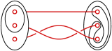
Figure 1: The deformation of observables corresponding to the implementation of a braid process on three anyons is shown. Configurations before and after are connected by world lines shown in red, while the charge observables are shown in black. This process relates two different ways of fusing the top two charges.

The defining difference between abelian and nonabelian anyon theories is that in an abelian theory particle content alone uniquely determines the outcome of joint charge measurements. In contrast, outcomes for nonabelian charge measurements depend on the history of the particles as well as their type. That is, the fusion space of a set of abelian anyons is one-dimensional, while it is generally larger for nonabelian anyons.

We consider a system supporting nonabelian Fibonacci anyon excitations, denoted by $\tau$. Two such anyons can have total charge that is either $\tau$ or $\mathbb{I}$ (vacuum), or any superposition of these, and so the fusion space in this case is 2-dimensional. We can represent basis states for this space using diagrams of definite total charge for the Wilson loops, and arbitrary states as linear combinations of these diagrams:

For $n$ anyons of type $\tau$, the dimension of the fusion space grows asymptotically as $\varphi^{n}$, where $\varphi=\frac{1+\sqrt{5}}{2}$ is the golden ratio.

Observables associated to non-intersecting loops commute, and so a basis for the space can be built from a maximal set of disjoint, nested loops. For three anyons, two possible ways of nesting loops are related via $F$-moves:

(1)

Here we have shown particles with charges $a$, $b$, and $c$ as well as total charge $d$. The lefthand side shows a state where the anyons with charge $a$ and $b$ are observed to have total charge $i$. The righthand side involves a superposition over total charge $j$ of the anyons with charge $b$ and $c$. The green line serves to linearly order the anyons, and track the history of braiding processes (see Ref. Burton (2016) for a more comprehensive discussion). It also denotes the direction along with $F$-moves occur. A clockwise braiding process, or half-twist, is effected by an $R$-move:

(2)

These diagrams can be composed (glued) by regarding the outermost observable as a charge in another diagram. This operation distributes over superpositions, and it also respects the $R$- and $F$-moves. Conversely, fusion of anyons corresponds to replacing the interior of a loop by a single charge.

For Fibonacci anyons, the non-trivial $R$ and $F$ moves are

$$R_{\mathbb{I}}^{\tau\tau}=\mathrm{e}^{\frac{-4\pi i}{5}}\ \ ,\ \ R_{\tau}^{\tau\tau}=\mathrm{e}^{\frac{3\pi i}{5}}\ \ ,\ \ F_{\tau}^{\tau\tau\tau}=\begin{pmatrix}\varphi^{-1}&\varphi^{-\frac{1}{2}}\\ \varphi^{-\frac{1}{2}}&-\varphi^{-1}\end{pmatrix}\,,$$

where the matrix is given in a basis labelled $(\mathbb{I},\tau)$. For more details of the Fibonacci anyon theory, see e.g. Ref. Nayak et al. (2008) and references therein.

In addition to the fusion space there is also a global degeneracy associated with the topology of the manifold on which the anyons reside. We consider systems with the topology of a torus, which for the Fibonacci anyons gives rise to a 2-fold degeneracy. This extra degree of freedom can be thought of being associated with the total anyonic charge (or flux) running through the torus itself. Since there are two different possible charges in the Fibonacci anyon model, the global degeneracy is 2.

I.2 Noise and error-correction

We consider encoding a qubit of quantum information in the global degeneracy associated with the topology of the manifold of our system. We endow this manifold with a finite set of $L\times L$ Wilson loops arranged in a square lattice tiling $\Lambda$. These tiles will be the observables accessible to the error-correction procedure (decoder). We can use these observables to construct an idealized Hamiltonian for this system of the form $H=-\sum_{t\in\Lambda}|{\mathbb{I}}\rangle\!\langle{\mathbb{I}}|_{t}\;,$ with $|{\mathbb{I}}\rangle\!\langle{\mathbb{I}}|_{t}$ the projector to charge $\mathbb{I}$ at tile $t$, i.e. the ground space of the model has vacuum total charge in each tile. Given the toroidal boundary conditions, this space is the two-fold degenerate codespace.

Typical thermal noise processes in this kind of system are pair-creation, hopping, exchange etc. of anyons. Such a model was analyzed in detail for Ising anyons in Ref. Brell et al. (2014). For convenience, in the numerical results presented in this study we will restrict to considering pair-creation events only, though all of our simulation techniques could be applied directly to the more general noise considered in Ref. Brell et al. (2014) as desired. It was seen in Ref. Brell et al. (2014) that the pair-creation-only setting was sufficient to capture the qualitative features of an error-correction simulation for the Ising anyons and we have no reason to expect that this would change when considering the Fibonacci anyon model.

Pair-creation events acting within a single tile do not affect the corresponding observable, and so the only pair-creation events we need explicitly consider act between neighboring pairs of tiles. These are then each associated with an edge of the lattice $\Lambda$, chosen uniformly at random to model high-temperature, short timescale thermalizing dynamics. In studies of codes based on abelian anyon models, the error correction threshold or memory lifetime is typically quoted in terms of an iid noise strength per edge. This measure is not appropriate in a nonabelian anyon setting, where noise processes on neighbouring edges do not commute. We thus measure the error correction threshold and memory lifetime in terms of the average number of noise processes per edge. It is easy to see that, in those cases where they are both appropriate, these two methods coincide in the limit of low error rates, and for the typical noise strengths we encounter in this paper, the discrepancy is around $10\%$ (see Ref. Brell et al. (2014) for more details).

We consider this treatment of anyon dynamics to be a phenomenological model in that it neglects any microscopic details of the system. This is consistent with the principles of topologically ordered systems and anyonic physics, where the key universal features describing the anyon model correspond to large length-scale physics, while the microscopic physics plays a less important (and non-universal) role. Note also that our analysis applies equally well to either a continuum setting, or to discrete lattice models supporting anyonic excitations.

In order to perform a logical error on our code, a noise process must have support on a a homologically nontrivial region of the manifold. These correspond to processes in which anyonic charge is transported around a non-trivial loop before annihilating to vacuum.

Our error-correction algorithm begins by measuring the charge on each tile of the lattice, producing a syndrome of occupied sites. Following this, it joins nearby occupied tiles into clusters, and measures the total charge within each cluster. Clusters with trivial charge are discarded, and then nearby clusters are merged (agglomeratively Hastie et al. (2009)). The merging process iterates at linearly increasing length scales, at each step measuring total charge and discarding trivial clusters, before concluding when there is at most a single cluster remaining (see Fig. 2). This decoder is based on a hierarchical clustering algorithm Hastie et al. (2009); Wootton and Hutter (2015), and follows a similar strategy to the hard-decision renormalization group decoder Bravyi and Haah (2013). The error-correction protocol and simulation procedure are discussed in more depth in Section IV.

Note that unlike the case of abelian anyons, the decoder cannot determine the charge of each cluster given only the syndrome information (as in Bravyi and Haah (2013)), and so must repeatedly physically query the system to measure these charges. Our simulation proceeds in this way as a dialogue between decoder and system, terminating when either the decoder itself terminates or when it performs a homologically nontrivial operation, thereby performing a potential logical error. Note that, as was found in Ref. Brell et al. (2014), we expect that our qualitative results may be reproduced by most alternative families of decoders, although it may not be clear in all cases how to extend these decoders to the nonabelian setting. The advantage of using a clustering decoder is its simplicity and flexibility, and the fact that its clustering scheme is compatible with the structure of the noise processes that allows us to classically simulate them.

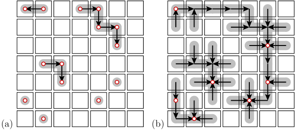
Figure 2: The decoder works by maintaining a set of disjoint clusters as rooted trees. (a) At the initial clustering stage, these trees are formed from neighboring sites that contain charges. Within each cluster, the charges are transported to the root of the tree (chosen arbitrarily), and their combined charge measured. The direction of transport (towards the root) is denoted by arrows. (b) At each successive round, all trees are grown in every direction, and overlapping trees are joined. Again, any charges within a cluster are transported to the root of the tree and measured. All clusters with vacuum total charge are deleted.

II Simulation

II.1 Classical simulability

Although simulating pair creation, braiding, and fusion of Fibonacci anyons is equivalent in computational power to universal quantum computing (and thus unlikely to be classically tractable), noise processes and error-correction procedures have structure that we can exploit to efficiently simulate typical processes of interest. In particular, those processes in which we expect error-correction to succeed are also those that we expect to be able to efficiently simulate for the following heuristic reasons (we leave a more rigorous analysis of simulability for noise and error correction processes as an open problem).

Below the (bond) percolation threshold for (say) a 2D square lattice, we expect random sets of bonds to decompose into separate connected components of average size $O(\log(L))$ and variance $O(1)$ Bazant (2000). Each noise process in our model is associated with a (randomly distributed) edge, and so disconnected components correspond to sets of anyons that could not have interacted at any point in their history. We are free to neglect the degrees of freedom associated with braiding between components because each component has trivial total charge. This allows us to simulate the braiding processes within each component separately. In other words: the quantum state in the fusion space of all anyons factorizes into a tensor product over components. Since each component has size only $O(\log(L))$, we can typically simulate these dynamics efficiently because the resulting fusion space has dimension $O(\mathrm{poly}(L))$. Of course, this is only a probabilistic statement, and so there may be cases where there exist components with size larger than $O(\log(L))$. However, the likelihood of this is suppressed exponentially in the lattice size $L$ Grimmett (1989).

However, random noise processes are not the only dynamics that we need to consider. We must also consider the effect of the error-correction routine itself. This acts iteratively to fuse anyons on increasing length scales. While this kind of fusion would typically merge components, forcing us to compute dynamics of larger and larger sets of anyons, large components are sparsely distributed (and thus unlikely to be merged), and in addition at each length scale the total number of anyons present is dramatically reduced by fusion, leading to a smaller number of anyons that must be simulated.

In the regime where the combined action of noise and error-correction does not percolate it is reasonable to expect that the simulation is efficient. However, with strong enough noise the state in the fusion space will no longer decompose at all and computing dynamics will become exponentially difficult in the system size. Nevertheless, we are able to simulate error-correction in the regime around the error-correction threshold for linear lattice sizes up to $L=128$.

II.2 Simulation algorithm

In order to track the state of the system we represent the state of the fusion space with a set of disjoint directed curves, one for each connected component with trivial total charge. Unlike previous work Brell et al. (2014), this creates a dynamically generated basis for the fusion space that allows for tensor factorization of disjoint components. A pair-creation noise process corresponds to the addition of an extra curve to the lattice, supporting two new anyons. Following the noise processes, our simulation must measure the total charge within each tile; the results of these measurements will form the error syndrome. This requires joining the curves that intersect that tile, and then performing $R$- and $F$-moves on the resulting curve so that all anyons within the tile have been localized within a contiguous region of the curve. An example of this procedure for a simple noise process is shown in Fig. 3. This procedure is discussed in more detail in Section IV, and the theoretical framework underlying it is expanded in Ref. Burton (2016). Braiding processes that encircle a non-trivial loop of our (toric) manifold can also be treated in an analogous way, following e.g. Ref. Pfeifer et al. (2012).

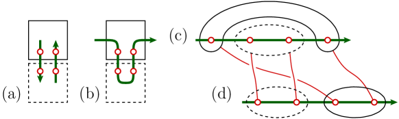
Figure 3: (a) Noise processes initially form isolated sets of pair-created anyons, each crossing the boundary of a tile. (b) To measure the total charge contained within each tile, we first join the participating curve diagrams arbitrarily into a single curve diagram. (c) The total charge of each tile can then be found by braiding anyons around each other until all charges within a tile are neighbors on the curve, as in (d). The red lines correspond to the worldlines for these braids.

Following the results of the charge measurements, the decoder determines a recovery operation that involves fusion of subsets of anyons. These fusions can be simulated and their results calculated in the same way, and the output charge placed at an appropriate point in the lattice. This procedure is iterated until either the decoder terminates successfully, or the simulation itself declares failure because the components become too large to analyze (roughly when they span the lattice).

III Results

III.1 Numerical results

We plot the performance of the decoder as a function of noise strength for varying lattice sizes in Fig. 4. The noise strength is parameterized by the Poisson process duration $t_{\mathrm{sim}}$, representing the expected number of errors per edge during the simulation. We find evidence of a decoding threshold below which decoding succeeds with asymptotic certainty as the system size increases at $t_{\mathrm{sim}}\simeq 0.125\pm 0.003$.

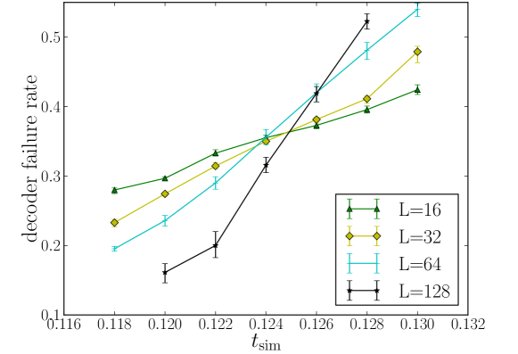
Figure 4: The decoder failure rate (a lower bound on the logical error probability) is shown as a function of simulation time for linear lattice sizes from $L=16$ to $128$. This provides strong evidence of threshold behavior at a critical memory lifetime of $t_{\mathrm{sim}}^{*}\simeq 0.125$. The existence of such a threshold implies that the Fibonacci anyon code simulated here is able to perfectly reliably store quantum information for times less than $t_{\mathrm{sim}}^{*}$ in the $L\to\infty$ limit.

We can guarantee that error-correction will succeed whenever the action of noise plus decoder does not percolate the anyons over the lattice, but it is possible that percolated events may still result in no error. The connection between the percolation threshold and the error-correction threshold is not well understood in general Hastings et al. (2014), though it is clear that our threshold estimate would be a lower bound for the true threshold that may be found if all events (including those that have percolated) were simulated. In any case, we do not expect this possible discrepancy to be significant in our simulations.

III.2 Discussion

We have demonstrated classical simulation of successful error correction in a universal anyon model. Though we have chosen several properties of our model and simulation in a convenient way for simplicity, Ref. Brell et al. (2014) presents good evidence that it is unlikely these choices will affect our results qualitatively. In particular, although we have considered a logical qubit encoded in the global topological degrees of freedom of our system, we could have encoded it in the fusion space of several preferred anyons. This situation would be appropriate to model error-correction routines for topological quantum computation. Additionally, we expect our results to be stable to changes in details of the noise model and decoding algorithm, again following Ref. Brell et al. (2014).

None of our techniques are restricted to simulation of Fibonacci anyon dynamics, and could equally well be used to simulate successful error-correction protocols in an arbitrary anyon code. As such, our methods could be used to demonstrate successful error-correction for an arbitrary anyonic topological quantum computer.

There are several interesting avenues for further research. Although it is not completely obvious how to do so, applying similar methods to more realistic models such as concrete microscopic spin models or models with non-topological features would give direct insight into practical error rates needed for nonabelian topological quantum memories. It would also be interesting to find classical spin models whose phase diagram encodes the threshold for error correction in these systems Dennis et al. (2002). Finally, an important extension of this work would be to the simulation of fault-tolerant error-correction protocols for nonabelian anyon codes.

IV Technical details

In order to estimate the error-correction threshold of Fibonacci anyon codes, we perform monte-carlo simulations of noise and recovery operations on systems of various sizes. For a given sample, the simulation can be broken down into several stages:

• Noise 

• Syndrome extraction 

• Decoding 

• Recovery 

After application of noise, the subsequent three steps (forming the error-correction routine) are iterated until success or failure, as will be described in more detail below.

It should be noted that while the noise, syndrome extraction, and recovery steps of this procedure are intended to really be a simulation of the physics of an anyon system, the decoding step is better thought of as an implementation of the classical processing that a successful error-correction experiment will require. Furthermore, the simulation of the noise and recovery steps will be rendered straightforward by the way we model our system in the first place. As such, the main novelty of our simulations is in the model itself, and the syndrome extraction step.

The key to simulating these processes effectively is the ability to describe topological operations by curve diagrams. This is an alternative representation of topological operations that is particularly suited to these kinds of numerical simulations of sparsely populated 2-dimensional anyon systems. The theoretical framework underpinning this description and the relation to to other representations of topological operations is discussed in Ref. Burton (2016).

In this section, we first describe our physical model of an anyon system and the corresponding noise, before showing how to simulate joint charge measurements (the core of syndrome extraction) within this model. The use of curve-diagrams is presented in an intuitive but ad-hoc way. Finally we describe our decoder and detail holistically how the different parts of the simulation interact.

IV.1 Physical model

We consider anyon systems defined on a torus. We endow this with a $L\times L$ square lattice of observables:

$$\Lambda:=\bigl{\{}\gamma_{ij}\bigr{\}}_{i,j=1,...,L}$$

These observables are the physically accessible charge observables that will be measured during syndrome extraction, before being passed to the decoder which will in turn determine physical recovery operations to be performed on the system. We call each $\gamma_{ij}$ a tile. In figures we show a small gap between the tiles but this is not meant to reflect an actual physical gap.

As noted above, the key to our model is to represent anyons and topological operations with curve diagrams. A curve diagram is a directed path that connects several anyons, which are denoted by preferred points along these paths. A curve diagram specifies a linear ordering of the anyons that allows us to define a basis for the corresponding fusion space, as well as to keep track of topological operations on this ordering. See Ref. Burton (2016) for a more formal introduction to curve diagrams.

The main noise processes we consider in our simulations are pair-creation events, though other topological processes such as hopping, exchange, etc. can also be implemented straightforwardly. The pair-creation process acts to populate the manifold with a randomly distributed set of anyon pairs, whose separation is much smaller than the size of a tile.

Each such pair will have vacuum total charge and so the observables $\gamma_{ij}$ will only be affected by pairs that cross a tile boundary, i.e. we need only consider distributing these pairs along edges of the tiles:

In simulating system undergoing noise for time $T$, we place a Poisson-distributed number of pair-creation events on the edges of tiles, with mean $2L^{2}T$.

In order to allow us to later calculate fusion outcomes for sets of anyons, in addition to locations of created anyons we also assign each pair a (directed) piece of curve, denoted in green. This curve can be thought of as a choice of fusion basis for the anyons along it. Since the total charge of any newly-created particle-antiparticle pair is vacuum, each of their fusion spaces can be treated independently. This results in our being able to consider independent disconnected curves for each such pair. We only need consider the joint state in the fusion space of different sets of anyons if they have interacted, and so it is with curve diagrams. Using this picture, it is easy to track the effects of moving anyons, which essentially are represented by appropriate extensions or deformations of the curve along which the anyon lies. These kinds of straightforward processes are all that are required to describe the noise and recovery steps of our simulation.

IV.2 Syndrome extraction

Syndrome extraction in this model corresponds to simulating measurements of the observables $\gamma_{ij}$, which represent the total charge contained within the corresponding tile. In order to compute measurement outcomes for the $\gamma_{ij}$ we first need to concatenate any two curve diagrams that participate in the same $\gamma_{ij}.$ Because each curve has vacuum total charge this can be done in an arbitrary way:

Working in the basis picked out by the resulting curve diagrams, we will show how to calculate measurement outcomes for each tile, the result of which is recorded on the original curve:

The basic data structure involved in the simulation we term a combinatorial curve diagram. Firstly, we will require each curve to intersect the edges of tiles transversally, and in particular a curve will not touch a tile corner.

For each tile in the lattice, we store a combinatorial description of the curve(s) intersected with that tile. Each component of such an intersection we call a piece-of-curve.

We follow essentially the same approach as taken in Abramsky (2007) to describe elements of a Temperley-Leib algebra, but with some extra decorations. The key idea is to store a word for each tile, comprised of the letters $\bigl{<}$ and $\bigr{>}$. Reading in a clockwise direction around the edge of the tile from the top-left corner, we record our encounters with each piece-of-curve, writing $\bigl{<}$ for the first encounter, and $\bigr{>}$ for the second. We may also encounter a dangling piece-of-curve (the head or the tail), so we use another symbol $*$ for this. The words for the above two tiles will then be $\bigl{<}\bigl{<}\bigr{>}\bigr{>}\bigl{<}\bigr{>}$ and $\bigl{<}\bigr{>}*\bigl{<}\bigl{<}\bigr{>}\bigr{>}.$ When the brackets are balanced, each such word will correspond one-to-one with an intersection of a curve in a tile, up to a continuous deformation of the interior of the tile, i.e. the data structure will be insensitive to any continuous deformation of the interior of the tile, but the simulation does not need to track any of these degrees of freedom.

We will also need to record various other attributes of these curves, and to do this we make this notation more elaborate in the paragraphs (I), (II) and (III) below. Each symbol in the word describes an intersection of the curve with the tile boundary, and so as we decorate these symbols these decorations will apply to such intersection points.

(I) We will record the direction of each piece-of-curve, this will be either an in or out decoration for each symbol. Such decorations need to balance according to the brackets. The decorated symbols $*_{\mbox{\tt in}}$ and $*_{\mbox{\tt out}}$ will denote respectively either the head or the tail of a curve. The words for the diagrams above now read as $\bigl{<}_{\mbox{\tt in}}\bigl{<}_{\mbox{\tt out}}\bigr{>}_{\mbox{\tt in}}\bigr{>}_{\mbox{\tt out}}\bigl{<}_{\mbox{\tt out}}\bigr{>}_{\mbox{\tt in}}$ and $\bigl{<}_{\mbox{\tt in}}\bigl{>}_{\mbox{\tt out}}*_{\mbox{\tt in}}\bigr{<}_{\mbox{\tt out}}\bigr{<}_{\mbox{\tt in}}\bigl{>}_{\mbox{\tt out}}\bigr{>}_{\mbox{\tt in}}.$

(II) We will record, for each intersection with the tile edge, a numeral indicating which of the four sides of the tile the intersection occurs on. Numbering these clockwise from the top as $1,2,3,4$ we have for the above curves: $\bigl{<}_{1}\bigl{<}_{2}\bigr{>}_{2}\bigr{>}_{3}\bigl{<}_{3}\bigr{>}_{4}$ and $\bigl{<}_{1}\bigr{>}_{1}*_{2}\bigl{<}_{3}\bigl{<}_{3}\bigr{>}_{4}\bigr{>}_{4}.$

(III) Finally, we will also decorate these symbols with anyons. This will be an index to a leaf of a (sum of) fusion tree(s). This means that anyons only reside on the curve close to the tile boundary, and so we cannot have more than two anyons for each piece-of-curve. The number of such pieces is arbitrary, and so this is no restriction on generality.

In joining tiles together to make a tiling we will require adjacent tiles to agree on their shared boundary. This will entail sequentially pairing symbols in the words for adjacent tiles and requiring that the in and out decorations are matched. Because the word for a tile proceeds conter-clockwise around the tile, this pairing will always reverse the sequential order of the symbols of adjacent tiles. For example, given the above two tiles we sequentially pair the $\bigl{<}_{\mbox{\tt out},2}\bigr{>}_{\mbox{\tt in},2}$ and $\bigr{>}_{\mbox{\tt out},4}\bigr{>}_{\mbox{\tt in},4}$ symbols with opposite order so that $\bigl{<}_{\mbox{\tt out},2}\sim\bigr{>}_{\mbox{\tt in},4}$ and $\bigr{>}_{\mbox{\tt in},2}\sim\bigr{>}_{\mbox{\tt out},4}.$

Note that in general, this will allow us to store the multiple disjoint curve diagrams that cover the lattice.

For each piece-of-curve, apart from a head or tail, there is an associated number we call the turn number. This counts the number of “right-hand turns” the piece-of-curve makes as it traverses the tile, with a “left-hand turn” counting as $-1.$ This number will take one of the values $-2,-1,0,1,2:$

IV.3 The paperclip algorithm

In order to calculate the total charge of each tile, we must transport all anyons within the tile until they are neighbours along their curve. In doing so, it will be convenient to consider transporting these anyons by moving them along tile edges. This is equivalent to a “refactoring” of the fusion space, as described in Ref. Burton (2016). We can further break down transport along the tile edge into a sequence of transports between neighbouring pieces of curve at that edge. The origin and destination of such a path now splits the curve diagram into three disjoint pieces which we term head, body and tail, where the head contains the endpoint of the curve, the tail contains the beginning of the curve and the body is the remainder. Here we consider transport forwards along the curve (from tail towards head), but the reverse case is analogous.

This arrangement is equivalent (isotopic) to one of four “paperclips”, which we distinguish between by counting how many right-hand turns are made along the body of the curve diagram. We also show an equivalent (isotopic) picture where the curve diagram has been straightened, and the resulting distortion in the anyon path:

In order to perform the desired transport, we must braid the anyon under consideration around the other anyons along the curve diagram. Denoting the sequence of anyons along the head, body and tail, $H,B$ and $T,$ respectively, and using $H^{r},B^{r}$ and $T^{r}$ to denote the same anyons with the reversed order, the appropriate braiding transformation ($R$-move) can be read off for each of the four paperclips:

$$-2: \ R[B]$$

$$-4: \ R[H^{r}]\ R[H]\ R[B]$$

$$+4: \ R[B]\ R[T]\ R[T^{r}]$$

$$+6: \ R[H^{r}]\ R[H]\ R[B]\ R[T]\ R[T^{r}]$$

where notation such as $R[B]$ is understood as sequentially clockwise braiding around each anyon in $B$.

Once all the anyons within a tile have been brought into a sequential piece of the curve, their total charge can easily be read off by an appropriate $F$-move. This allows us to perform syndrome extraction, by repeating this procedure for each tile of the lattice.

IV.4 Decoding and error-correction

After the noise process is applied to the system, the error correction routine attempts to annihilate all the anyons on the lattice in a way that does not affect the encoded information. It proceeds as a dialogue between the decoder and the system. The syndrome extraction procedure provides information to the decoder, which suggests a recovery procedure, the results of which are found by a subsequent syndrome extraction step, and so on. This iterative procedure continues until the extracted syndrome is empty (i.e. i.e. there are no remaining anyons on the lattice), or the decoder declares failure. Here we show this in a process diagram, with time running up the page:

So far we have discussed the simulation of the (quantum) system and now we turn to the decoder algorithm. This is similar to other clustering-type decoders used in the literature Bravyi and Haah (2013), in that it attempts to form and fuse together clusters of anyons on larger and larger length scales, declaring failure if anyons remain after fusion at the largest length scale. Our simulation also declares failure if at any point the curve diagrams describing the state of the system form a homologically non-trivial loop (span the lattice), this being a necessary condition for error-correction failure.

The structure of the error-correction routine is as follows, and will be illustrated by an example below.

 1:  def error_correct():
 2:      syndrome = get_syndrome()
 3:
 4:      # build a cluster for each charge
 5:      clusters = [Cluster(charge) for charge in syndrome]
 6:
 7:      # join any neighbouring clusters
 8:      join(clusters, 1)
 9:
10:      while clusters:
11:
12:          # find total charge on each cluster
13:          for cluster in clusters:
14:              fuse_cluster(cluster)
15:
16:          # discard vacuum clusters
17:          clusters = [cluster for cluster in clusters if non_vacuum(cluster)]
18:
19:          # grow each cluster by 1 unit
20:          for cluster in clusters:
21:              grow_cluster(cluster, 1)
22:
23:          # join any intersecting clusters
24:          join(clusters, 0)
25:
26:      # success !
27:      return True

First, we show the result of the initial call to get_syndrome(), on line 2. This is computed using the syndrome extraction step as described above. The locations of anyon charges are highlighted in red. For each of these charges we build a Cluster, on line 5. Each cluster is shown as a gray shaded area.

The next step is the call to join(clusters, 1), on line 8, which joins clusters that are separated by at most one lattice spacing. We now have seven clusters:

Each cluster is structured as a rooted tree, as indicated by the arrows which point in the direction from the leaves to the root of the tree. This tree structure is used in the call to fuse_cluster(), on line 14. This moves anyons in the tree along the arrows to the root, fusing with the charge at the root. This movement of anyons is a physical recovery operation that is easily simulated by extending the curve diagram along the transport path, and moving the anyons along it.

For each cluster, the charge is then measured using the syndrome extraction procedure, and the resulting charge at the root is taken as the charge of that cluster. Any cluster with vacuum total charge is then discarded (line 17). In our example, we find two clusters with vacuum charge and we discard these. The next step is to grow the remaining clusters by one lattice spacing (line 20-21), and join (merge) any overlapping clusters (line 24).

Note that we can choose the root of each cluster arbitrarily since we are only interested in the total charge of each cluster, and also that for simplicity we have neglected the boundary of the lattice in this example.

We repeat these steps of fusing, growing and then joining clusters (lines 10-24.) If at any point this causes a topologically non-trivial operation, the simulation aborts and a failure to decode is recorded. Otherwise we eventually run out of non-vacuum clusters, and the decoder succeeds (line 27).

By repeatedly performing this simulation of noise and error-correction on different sized lattices, and for different noise rates (or memory lifetimes), we are able to estimate the error-correction threshold for this type of system.