Maximizing the detection probability of kilonovae associated with gravitational wave observations

Abstract

Estimates of the source sky location for gravitational wave signals are likely span areas ranging up to hundreds of square degrees or more, making it very challenging for most telescopes to search for counterpart signals in the electromagnetic spectrum. To boost the chance of successfully observing such counterparts, we have developed an algorithm which optimizes the number of observing fields and their corresponding time allocations by maximizing the detection probability. As a proof-of-concept demonstration, we optimize follow-up observations targeting kilonovae using telescopes including CTIO-Dark Energy Camera, Subaru-HyperSuprimeCam, Pan-STARRS and Palomar Transient Factory. We consider three simulated gravitational wave events with $90\%$ credible error regions spanning areas from ${\sim}30\,\mathrm{deg^{2}}$ to ${\sim}300\,\mathrm{deg^{2}}$. Assuming a source at $200\,\mathrm{Mpc}$, we demonstrate that to obtain a maximum detection probability, there is an optimized number of fields for any particular event that a telescope should observe. To inform future telescope design studies, we present the maximum detection probability and corresponding number of observing fields for a combination of limiting magnitudes and fields-of-view over a range of parameters. We show that for large gravitational wave error regions, telescope sensitivity rather than field-of-view, is the dominating factor in maximizing the detection probability.

I. Introduction

The detection of gravitational waves from the inspiral and merger of binary black-hole systems (Abbott et al., 2016a, b) has marked the beginning of the GW astronomy era. With the advanced interferometric detectors, GWs are expected to be observed from a number of additional source types including the mergers of binary neutron stars (BNS), and neutron star-black hole (NSBH) systems. For these other sources the presence of matter from the neutron stars (NS) components, in such a violent interaction with its companion, makes it likely that electromagnetic (EM) emission will be generated. The joint detection of a GW signal and its EM counterpart is therefore of particular interest. A coincident EM observation together with the detection of GWs from these sources would lead to a deeper and more comprehensive understanding of these objects. A successful EM follow-up observation triggered by a GW event can greatly improve the identification and localization of the host galaxy, bring us a more accurate estimate of the distance and energy involved, and provide better understanding of the merger’s hydrodynamics and the local environment of the progenitor (Bloom et al., 2009; Kulkarni & Kasliwal, 2009; Phinney, 2009). Additionally, knowledge obtained by EM follow-up observations may break the modeling degeneracies of binary properties, and confirm the association between the GW source and its EM counterpart. Also, successfully locating the EM counterpart of a GW event could increase the confidence in the GW detection (Blackburn et al., 2015).

Among many other potential EM counterparts of GW events, it has been argued that kilonovae are a strong candidate for GW signals from BNS and NSBH mergers (Li & Paczynski, 1998; Metzger & Berger, 2011; Tanvir et al., 2013; Li et al., 2016). We therefore focus our discussion on kilonovae only. Kilonovae are predicted to produce an optical/infrared and isotropic quasi-thermal transient, and thought to originate from the hot neutron-rich matter ejected from BNS mergers. This ejection triggers r-process nucleosynthesis, the radioactive decay of which sustains the high temperature of the ejecta and powers the kilonovae. Kilonovae can be ${\sim}1000$ times brighter than a nova (peak luminosity $L\sim 10^{40}\,\mathrm{erg/s}$) (Metzger et al., 2015), but given the expected rate of BNS events, their corresponding distances make kilonovae relatively dim EM transients. In addition, according to Metzger & Berger (2011), a kilonova maintains its peak luminosity only for hours to days after merger. However, more recent calculations including the opacity of the $r-process$ elements (Barnes & Kasen, 2013; Tanaka et al., 2014; Grossman et al., 2014) indicate that this timescale is likely to be days to weeks. Currently, there are three detections associated with the short-duration gamma-ray bursts GRB 130603B (Tanvir et al., 2013; Berger et al., 2013) and GRB 060614 (Yang et al., 2015; Jin et al., 2015) and GRB 050709 (Jin et al., 2016).

The sky location estimate for a GW event can cover a large fraction of the sky (${\gtrsim}100\,\mathrm{deg^{2}}$ (Singer et al., 2014)), posing a significant challenge to telescopes with fields of view of order ${\sim}1\,\mathrm{deg^{2}}$ trying to find counterpart signals in the EM spectrum. Observing and confidently detecting kilonovae demands long exposure times even for powerful telescopes. It has been proposed that the infrared sensitivity of the planned James Webb Space Telescope (JWST) may enable detections with short exposure times, thus compensating for its small FOV (Bartos et al., 2015b). The use of galaxy catalogs may also provide prior information on the direction of an event (Fan et al., 2014; Bartos et al., 2015a; Gehrels et al., 2016). Nonetheless, even with JWST and galaxy catalogs, the observation time can still span an entire night, which may make target-of-opportunity BNS merger observations less attractive.

Given that current and future EM telescopes will be subject to limited observational resources, we might ask how can we maximize the detection probability of a GW triggered kilonova signature. We have developed an algorithm to answer this question, and here we present the results of a proof-of-concept demonstration applied to four different telescopes including Subaru-HyperSuprimeCam (HSC) (Miyazaki et al., 2012) , CTIO-Dark Energy Camera (DEC) (Bernstein et al., 2012), Pan-Starrs (Kaiser et al., 2002), and Palomar Transient Factory (PTF) (Law et al., 2009) for three different simulated GW events. This algorithm takes as inputs GW sky localization information, and returns a guidance strategy for time allocation and telescope pointing for a given EM telescope. In this paper we restrict the discussion to kilonovae from BNS mergers and leave the discussion of kilonova from NSBH for future study. This is in part due to the fact that our chosen GW data set from Singer et al. (2014) contains only BNS mergers. However, we remind the readers that there is no theoretical restriction preventing us from applying our algorithm using other EM counterpart models and neither is it restricted to using only GW sky maps from compact binary coalescence (CBC) events.

This paper is organized as follows: the methodology is introduced in Section II and we describe the implementation in Section III. The results obtained with the algorithm and a discussion of these results are given in Section IV. The possible future directions of this work are provided in Section VI, and our conclusions are presented in Section VII.

II. Methodology

As a proof-of-concept of our general EM follow-up method, here we have chosen to focus on kilonovae counterpart signatures. We have also adopted some simplifications which will be relaxed in future studies. We assume that the available observation time is short compared to the luminosity variation timescale of a kilonova. This is validated by the fact that kilonova’s luminosity variation timescale is estimated to be $\sim$days to a week, which is longer than a reasonable continuous EM observation. This approximation allows us to assume that a kilonova has constant luminosity during the observation period. We also only consider the use of R-band luminosity information, while the method presented can be extended to other regions of the EM spectrum. In reality, identifying a target EM counterpart requires tracking the object’s light curves, leading to several observations of the same point in the sky over several days. However, in this work we deal with the problem of detection, rather than identification. We consider only single observations and calculate optimized pointing directions and durations for a constrained total observation length and constant luminosity. Subsequent observations for the purpose of identifying variation within a field can be achieved by repeating our proposed observing strategy at some later time.

In general, GW events could be localized to ${\gtrsim}100\,\deg^{2}$, which is much larger than a typical EM telescope’s FOV (${\lesssim}1\,\deg^{2}$). We therefore do not consider the telescope’s rotation around its own axis, hence throughout this work, reference to single telescope pointing implies a rectangular Charge-coupled device (CCD) image with edges parallel to lines of longitude and circles of latitude.

We also assume that the prior information from a GW trigger can be approximated as having independent sky location and distance probability distributions. Generally, this may not be the case, however, our mathematical treatment can be greatly simplified under this assumption. We note that the sky maps available for our chosen dataset (discussed in Sec. III) naturally lend themselves to this approximation since no distance information was computed as part of the rapid sky localization study reported in Singer et al. (2012). The final assumption is that the EM telescope can see every direction regardless of the location of the Sun, Moon, and the horizon. The issue of optimization of EM follow-up observations under the time-critical constraints such as those imposed by a source dipping below the horizon is explored in Rana et al. (2016).

II.1. Bayesian Framework

We use $D_{\text{EM}}$ to denote the successful detection of an EM counterpart. The probability of this occurring depends on the size of the selected telescope’s FOV $\omega$, the observed sky locations$(\alpha,\delta)$, and the exposure time $\tau$. The posterior probability of successful detection is then given by

$$P(D_{\mathrm{EM}}|\omega,\tau,I)=\int_{N^{*}}^{\infty}dN~{}p(N|\omega,\alpha,\delta,\tau,I).$$ (1)

Here, $I$ is prior information that includes the selected telescope’s parameters, such as its photon collecting area $\mathrm{A}$, filter and CCD efficiency. For a particular observation the number of photons $N$ collected by the telescope is

$$N=10^{\frac{25-m}{2.5}}\times\left(\tau A\right)$$ (2)

where $m$ is the apparent magnitude of the observed source. The threshold count $N^{*}$ is the criterion for detection determined by the signal-to-noise ratio (SNR) threshold, background noise and the selected telescope’s sensitivity. The value of $N^{*}$ is given by Eq. 2 with input values of $m$ and $\tau$ corresponding to the selected telescope’s detection threshold (see Table 1). The constant $10^{10}$ in Eq. 2 is the number of photons per second at $m=0$. In practice, the value of $N^{*}$ should also account for the change in background light accumulated for different choices of observation time $\tau$, however, for simplicity we ignore this effect in this work. Since the number of photons expected from a target EM counterpart depends on its absolute magnitude $M$, distance $R$ from the telescope, and how likely that the GW event is located within the field being observed, Eq. 1 can be expanded such that

$$P(D_{\mathrm{EM}}|\omega,\tau,I)=\int_{N^{*}}^{\infty}dN\int dM\int dR\times$$

$$\int_{\omega}d\alpha\,d\delta~{}p(N|M,R,\tau,I)p(M|I)p(\alpha,\delta,R|I).$$ (3)

The quantity $P(N|M,R,\tau,I)$ is the probability of receiving $N$ photons from a source, given its absolute magnitude $M$, distance $R$, and observation time $\tau$, and is described by a Poisson distribution. Since we assume that the prior distribution on the distance to the target EM counterpart is statistically independent of the prior distribution on its sky location, Eq. II.1 can be written as

$$P(D_{\mathrm{EM}}|\omega,\tau,I)=P_{\mathrm{GW}}(\omega)\times P_{\mathrm{EM}}(\tau)$$ (4)

where,

$$P_{\mathrm{GW}}(\omega) = \int_{\omega}p(\alpha,\delta|I)d\alpha\,d\delta,$$ (5a)

$$P_{\mathrm{EM}}(\tau) = \int dM\int dR\int_{N^{*}}^{\infty}dN$$ (5b)

$$p(N|M,R,\tau,I)p(R|I)p(M|I).$$

Table 1Telescope parameters

Telescope	Aperture	FOV	Exposure	Sensitivity	$N^{*}/A$
	(m)	(deg2)	(s)	(5-$\sigma$ mag
				in R-band)	(m-2)
DEC	4.0	3.0	50	23.7	162.0
HSC	8.2	1.13	30	24.5	46.5
Pan-Starrs	1.8	7.0	60	22.0	930.5
PTF	1.2	7.0	60	20.6	3378.3
LSST	6.7	9.6	15	24.5	23.26

It should be noted that the GW sky localization information used for this work has been marginalized over distance, meaning that the GW information represents a 2D error region projected onto the sky. However, since the distance estimate inferred from a GW observation will typically be poorly constrained and can be well approximated by a Gaussian distribution (Veitch et al., 2015; Singer et al., 2016), we assume a Gaussian prior with mean $=200\mathrm{Mpc}$ and standard deviation $=60\mathrm{Mpc}$ for the distance. In principle any form of positional information can be incorporated into our analysis and therefore our method can be adapted to include more realistic GW distance information. It is also possible that further constraints from galaxy catalogs can also be incorporated into our method (Fan et al., 2014).

We assume the least informative prior on peak luminosity such that $p(L|I)\propto L^{-\frac{1}{2}}$. It then follows that the prior on peak magnitude is given by

$$p(M|I)\propto 10^{-\frac{M}{5}}$$ (6)

where we assume $M$ has a prior range of $(-13,-8)$ as defined by the peak magnitudes of the models in Barnes & Kasen (2013).

The probability of EM detection as defined in Eq. 1 considers only one observing field. Given the size of a GW sky localization error region, and the typical size of an EM telescope’s FOV, the number of fields needed to be considered is ${>}1$. If an error region enclosing $90\%$ of the GW probability covers $S\,\mathrm{deg^{2}}$ and the EM telescope FOV is $w\,\mathrm{deg^{2}}$, the maximum number $n$ of fields required to cover the error region at $90\%$ can be estimated as $n{\lesssim}S/\omega$.

One might assume that observing as many fields as possible is optimal but we will show that telescope time is better spent by observing $k$ fields where $k$ lies in the range $[1,n]$. This occurs when it becomes more beneficial to observe a particular field for longer than observing a new field.

For a given total observation time $T$, we are free to choose which fields we observe and the observation time allocated to each field. We represent these quantities by the vectors $\{\omega^{(k)}\}$ and $\{\tau^{(k)}\}$ respectively where $k$ is the total number of chosen fields. Maximizing the detection probability of a kilonova amounts to finding the values of these vectors and the value of $k$ which maximizes:

$$P(D_{\mathrm{EM}}|k) \equiv P(D_{\mathrm{EM}}|\{\omega^{(k)}\},\{\tau^{(k)}\},I)$$ (7)

$$\equiv \sum_{i=1}^{k\leq n}P(D_{\mathrm{EM}}|\omega^{(k)}_{i},\tau^{(k)}_{i},I).$$

The choices of $\{\tau^{(k)}\}$ are subject to the constraint that

$$kT_{0}+\sum_{i=1}^{k}\tau^{(k)}_{i}=T,$$ (8)

where $T_{0}$ represents the time required to slew between telescope pointings and/or perform CCD readout, and is equal to $\mathrm{max}(\mathrm{slew~{}time,CCD~{}readout~{}time})$. We treat $T_{0}$ as independent of the angular distance between pointings.

The expression we have for kilonova detection probability (Eq. 7) as a function of the number of observed fields depends on our choice of field location and observation time within each field. Given a number of fields $k$ we begin choosing fields with a greedy algorithm, which will be described in section III. Once the $k$ fields have been chosen, they are represented by $\{\omega^{(k)}\}$ and Eq. 7 is maximized over the parameter vector $\{\tau^{(k)}\}$ to obtain the optimal kilonova detection probability. This is then repeated for each $k$ in the range $[1,n]$ to find the optimal number of observed fields $k$.

III. Implementation

In this section we describe the processes for applying the GW sky localization information and generating the optimal observing strategy. The flow chart in Fig. 1 is a visual representation of this process.

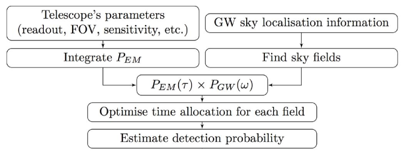
Figure 1.— The process for generating an optimized observing strategy. Our algorithm takes two inputs: the GW sky localization information and a set of telescope parameters. After integrating over the number of received photons $N$, the source distance $R$, and the source absolute magnitude $M$, the algorithm returns the probability of detection of an EM kilonova signal $P_{\mathrm{EM}}$ as a function of the field observation time $\tau$. In parallel, for each choice of the total number of observed fields $k$, the algorithm selects the fields using a greedy algorithm. Based on the enclosed GW probability within each field the corresponding optimized observation times are computed using a Lagrange Multiplier approach. The total EM detection probability is then output for each choice of k.

As shown in Fig. 1, we require information regarding the sky position of the GW source which we obtain from the BAYESTAR algorithm (Singer & Price, 2016). This algorithm outputs GW sky localization information using a HEALPix coverage of the sky. Each HEALPix point corresponds to a value of the GW probability and represents an equal area of the sky. BAYESTAR can rapidly (in ${\sim}10$s) generate event location information and has been shown in Singer et al. (2014) to closely match results from more computationally intensive off-line Bayesian inference methods (Veitch et al., 2015). The simulated GW events used in this work are from BNS systems and taken directly from the dataset used in Singer et al. (2014).

In this work, we consider follow-up observations using four telescopes (HSC, DEC, Pan-Starrs, and PTF) for three simulated representative GW events (see Table 2) which are studied assuming three total observation times $T=2,4,6\,\mathrm{hrs}$. For any telescope, GW event and total observation time the first stage of our procedure is to calculate the maximum number of fields $n$ required to cover the sky area enclosed by the $90\%$ probability contour of the GW sky region.

In order to identify the possible observing fields for a given GW event, the greedy algorithm identifies the least number of HEALPix locations on the sky whose sum of GW probability is equal to the desired confidence level (in our case $90\%$). Then, assuming that each of those points represents the center of an observing field we compute the sum of GW probability from each HEALPix point whose center lies within each of those fields. The field returning the maximum sum of the GW probability among those fields will be the first field. Subsequent fields are found by the same procedure, with the HEALPix points in the previous fields ignored. The summed probability within each field is an accurate approximation to the quantity $P_{\text{GW}}(w)$ as defined in Eq. 5a. The $n$ selected fields are labeled in the order with which they are chosen and hence their label indicates their rank in terms of enclosed GW probability. Therefore the first $k\leq n$ fields represent our optimized choice of the values of $\{\omega^{(k)}\}$ in Eq. 7.

As shown in Eqns. 4, 5b and 7, the detection probability achieved by observing $k$ selected fields can be expressed as the sum of the product of the EM and GW probabilities in each field. For each value of $k$ in the range $[1,n]$ we apply a Lagrange Multiplier to find the solution for the values $\{\tau^{(k)}\}$ that maximizes the detection probability given by Eq. 7. This is subject to the constraints defined in Eq. 8 and the value of $k$ that returns the highest detection probability is identified as the optimal solution. The analysis therefore guides us as to which subset of fields should be observed with the selected telescope and how much time should be allocated to each of those selected fields given the total observation time constraint.

IV. Results

In this section we present the results of our algorithm using our four example telescopes applied to the follow up of three simulated GW events. These events are taken from the dataset used in (Singer et al., 2014) and are designated with the IDs 28700, 19296 and 18694. The error regions for these events each cover ${\sim}300\,\mathrm{deg^{2}}$, ${\sim}100\,\mathrm{deg^{2}}$, and ${\sim}30\,\mathrm{deg^{2}}$ respectively and details of these events are presented in Table 2. These events were chosen to represent the potential variation in sky localization ability of a global advanced detector network. We highlight that the actual injected distances for our chosen events are $51\,\mathrm{Mpc}$, $27\,\mathrm{Mpc}$ and $12\,\mathrm{Mpc}$ respectively, while for our analysis we have assumed a distance of $200\,\mathrm{Mpc}$ for each event. However, the validity of this work is not undermined. The injected events were originally simulated assuming a 2 detector aLIGO First Observational Run configuration. Our analysis assumes a 2(3) detector design sensitivity aLIGO configuration. The SNR and sky localization for an event at $200\,\mathrm{Mpc}$ in the latter configuration is comparable (to within factors of ${\sim}$few) to events at a few tens $\mathrm{Mpc}$ for the former configuration.

Table 2Simulated GW event parameters.

Event ID1	SNR	90% Region	Chirp Mass
		$(\mathrm{deg^{2}})$	$(M_{\odot})$
28700	16.8	302	1.33
19296	24.3	103	1.28
18694	24.0	28.2	1.31

Figure 2 shows the optimized tiling of observing fields obtained using the greedy algorithm approach. For each telescope we show sky maps of the GW probability overlaid with the $90\%$ coverage tiling choices for the three representative GW events. The FOV’s of the telescopes range from $1.13\,\text{deg}^{2}$ to $7.1\,\text{deg}^{2}$ and as such the required number and location of tilings differ accordingly. The largest and smallest number of observation tilings are 230 and 7 for the largest GW error region (ID 28700) using HSC and for the smallest error region (ID 18694) using either Pan-Starrs or PTF respectively.

Each of the event maps are the result of an analysis assuming only 2 GW detectors. Without a third detector the sky location of an event is restricted to a thin band of locations consistent with the single time delay measurement between detectors. This degeneracy is partially broken with the inclusion of antenna response information resulting in extended arc structures. The third event that we consider (ID 18694) has sufficient SNR and suitable orientation with respect to the detector network that even with 2 detectors the sky region is well localized and is only partially extended. We consider this event to be approximately representative of sky maps obtained from a 3 detector network. We also note that given the imperfect duty factors of both the initial and advanced detectors it is highly likely that future detections will be made whilst one or more detectors are offline. We therefore use the first 2 example events (ID 28700 and 19296) as simultaneously representative of such a 2-detector scenario and of the potential situation in which a third detector is significantly less sensitive than the other two.

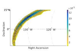
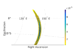
(a) $90\%$ coverage tilings used for the HSC telescope.

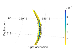
(b) $90\%$ coverage tilings used for the DEC telescope.

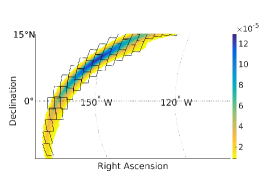
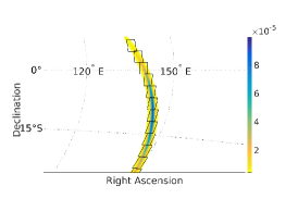
(c) $90\%$ coverage tilings used for the Pan-Starrs telescope.

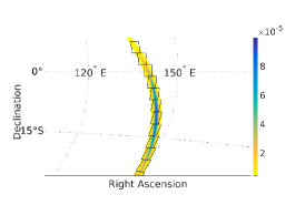
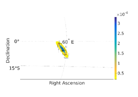
(d) $90\%$ coverage tilings used for the PTF telescope.

Figure 2.— The optimized locations of the observing fields covering $90\%$ of the GW probability for each telescope and for each of the 3 simulated GW events. Each row of plots corresponds to the 4 different telescopes (a) HSC, (b) DEC, (c) Pan-Starrs, and (d) PTF. Within each row we show the optimized observing field locations for the ${\sim}300\,\text{deg}^{2}$ event (ID 28700) on the left, the ${\sim}100\,\text{deg}^{2}$ event (ID 19296) in the center, and the ${\sim}30\,\text{deg}^{2}$ event (ID 18694) on the right. In each plot the GW sky error is shown as a shaded region with the color bar indicating the value of posterior probability density.

Figures 3, 4 and 5 display the results of the simulated EM follow-up observations for the events labeled 28700, 19296 and 18694 respectively. From the top panels to the bottom panels, the assumed total observation times are 6 hrs, 4 hrs and 2 hrs. The plots on the left of the figure show the optimized detection probability $P(D_{\mathrm{EM}}|k)$ as a function of the total observed number of fields $k$. The plots on the right of the figure display the optimal time allocations corresponding to the value of $k$ returning the highest detection probability (indicated by a circular marker in the detection probability plots on the left of the figure). The indices refer to the labels assigned to the fields when being chosen by the greedy algorithm.

We highlight the asymptotic behavior of the detection probability curves in Figs. 3, 4 and 5. This is due to a particular feature of our algorithm and is explained as follows. As the number of fields are increased we approach an optimal value $k^{*}$ where to observe an addition field with any finite observation time would actually reduce the detection probability. This occurs where the gains from an additional field are outweighed by the losses incurred by reducing the lengths of the observations of the other fields. In this case, for a given value of $k$ above the optimal value the optimal choice is to allocate $\tau=0$ to all fields with index greater than $k^{*}$. If we know that we will allocate no time to these fields then we also have no need to slew to them or to readout from the CCD. Hence the optimal time allocations and also detection probability for values of $k>k^{*}$ remains constant at the maximum value.

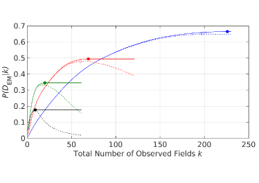
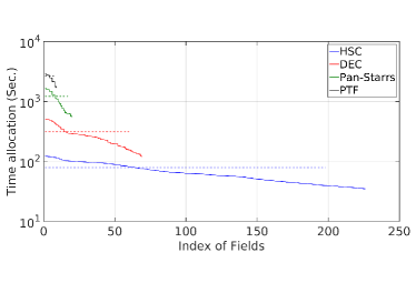
(a) EM detection probability and optimized observation times for $T=6$ hour total observation times.

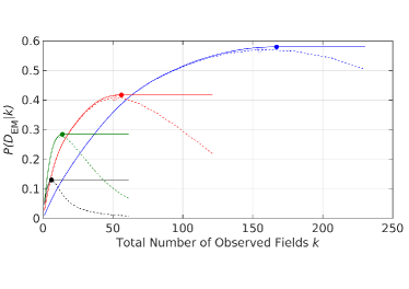
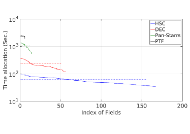
(b) EM detection probability and optimized observation times for $T=4$ hour total observation times.

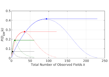
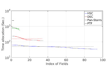
(c) EM detection probability and optimized observation times for $T=2$ hour total observation times.

Figure 3.— The results of simulated EM follow-up observations for the ${\sim}300\,\text{deg}^{2}$ GW event (ID 28700). We show the optimized EM detection probability as a function of the number of observing fields (left) and the allocated observing times for the optimal number of fields (right). The subfigures (a), (b) and (c) show results from 3 different total observation times for 6 hrs, 4 hrs and 2 hrs, respectively. For each total observation time the 4 solid curves in each plot correspond to the optimal time allocation strategy applied to each of the 4 telescopes. The dashed lines show results for the equal time strategy. The solid markers and the circles indicate the number of observing fields at which the maximum detection probability is achieved using the optimal time allocation strategy and the equal time strategy respectively.

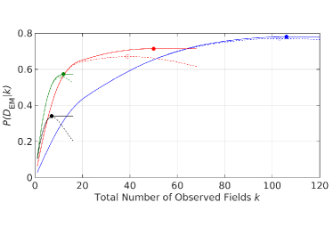
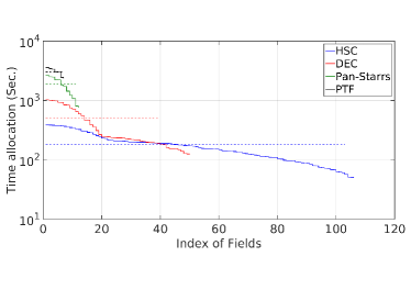
(a) EM detection probability and optimized observation times for $T=6$ hour total observation times.

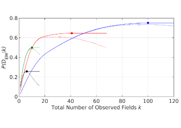
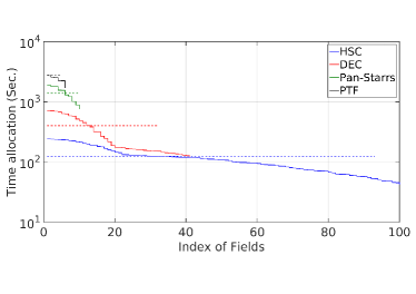
(b) EM detection probability and optimized observation times for $T=4$ hour total observation times.

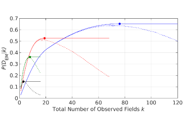
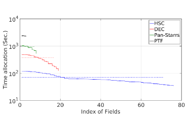
(c) EM detection probability and optimized observation times for $T=2$ hour total observation times.

Figure 4.— The results of simulated EM follow-up observations for the ${\sim}100\,\text{deg}^{2}$ GW event (ID 19296). We show the optimized EM detection probability as a function of the number of observing fields (left) and the allocated observing times for the optimal number of fields (right). The subfigures (a), (b) and (c) show results from 3 different total observation times for 6 hrs, 4 hrs and 2 hrs, respectively. For each total observation time the 4 solid curves in each plot correspond to the optimal time allocation strategy applied to each of the 4 telescopes. The dashed lines show results for the equal time strategy. The solid markers and the circles indicate the number of observing fields at which the maximum detection probability is achieved using the optimal time allocation strategy and the equal time strategy respectively.

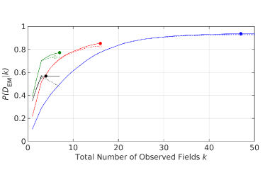
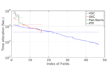
(a) EM detection probability and optimized observation times for $T=6$ hour total observation times.

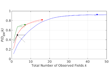
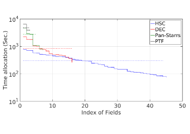
(b) EM detection probability and optimized observation times for $T=4$ hour total observation times.

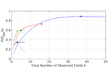
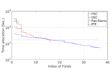
(c) EM detection probability and optimized observation times for $T=2$ hour total observation times.

Figure 5.— The results of simulated EM follow-up observations for the ${\sim}30\,\text{deg}^{2}$ GW event (ID 18694). We show the optimized EM detection probability as a function of the number of observing fields (left) and the allocated observing times for the optimal number of fields (right). The subfigures (a), (b) and (c) show results from 3 different total observation times for 6 hrs, 4 hrs and 2 hrs, respectively. For each total observation time the 4 solid curves in each plot correspond to the optimal time allocation strategy applied to each of the 4 telescopes. The dashed lines show results for the equal time strategy. The solid markers and the circles indicate the number of observing fields at which the maximum detection probability is achieved using the optimal time allocation strategy and the equal time strategy respectively.

As a comparison, we introduce a second observing strategy for time allocation in which all the fields are observed with equal time. We call this method the equal time strategy. For each value of $k$, subject to the total observation time constraints and slew/readout time, the time allocated to each field is given by $T/k-T_{0}$. The values of $P(D_{\mathrm{EM}}|k)$ obtained using this strategy are plotted as dashed lines in the plots on the left of Figs. 3, 4 and 5. The time allocations corresponding to the peaks of the dashed lines are plotted as flat lines (constant equal values) in the plots on the right of the figures. The resultant maximal probabilities and corresponding optimal number of fields for both time allocation strategies are given in Table 3 for all simulated events and total observation times. We also indicate the relative gains in detection probability obtained using our fully optimized (Lagrange multiplier) approach relative to the equal time strategy.

Table 3The EM detection probability using both the optimal and equal time strategies

Telescope	Event ID	Strategy	EM detection probability (optimal number of fields)						Relative Gain
			6 hrs		4 hrs		2 hrs		6 h	4 h	2 h
HSC	28700	LM	66.4%	(226)	58.0%	(167)	41.6%	(94)	1.4%	1.0%	0.3%
		ET	65.0%	(198)	57.0%	(155)	41.3%	(90)
	19296	LM	78.1%	(106)	75.1%	(100)	65.3%	(76)	1.1%	1.4%	1.6%
		ET	77.0%	(103)	73.7%	(93)	63.7%	(71)
	18694	LM	93.7%	(47)	92.7%	(45)	89.1%	(37)	0.8%	1.2%	1.7%
		ET	92.9%	(47)	91.5%	(44)	87.4%	(36)
DEC	28700	LM	49.4%	(69)	41.7%	(56)	28.1%	(35)	1.4%	1.0%	0.5%
		ET	48.0%	(60)	40.7%	(51)	27.6%	(34)
	19296	LM	71.5%	(50)	64.7%	(41)	52.6%	(19)	4.3%	3.8%	1.1%
		ET	67.2%	(39)	60.9%	(32)	51.5%	(17)
	18694	LM	85.3%	(16)	81.7%	(16)	73.0%	(16)	2.3%	3.0%	3.9%
		ET	83.0%	(16)	78.7%	(16)	69.1%	(13)
Pan-Starrs	28700	LM	34.6%	(20)	28.5%	(14)	19.0%	(9)	1.2%	0.5%	0.2%
		ET	33.4%	(17)	28.0%	(13)	18.8%	(9)
	19296	LM	57.4%	(12)	50.1%	(10)	36.2%	(8)	1.5%	1.0%	0.4%
		ET	55.9%	(11)	49.1%	(10)	35.8%	(7)
	18694	LM	77.2%	(7)	71.5%	(7)	59.7%	(5)	4.0%	3.7%	1.4%
		ET	73.2%	(6)	67.8%	(5)	58.3%	(3)
PTF	28700	LM	17.7%	(9)	13.0%	(6)	7.1%	(3)	0.2%	0.1%	0.0%
		ET	17.5%	(8)	12.9%	(6)	7.1%	(3)
	19296	LM	34.1%	(7)	25.8%	(6)	14.6%	(3)	0.3%	0.2%	0.0%
		ET	33.8%	(7)	25.6%	(5)	14.6%	(3)
	18694	LM	56.9%	(4)	50.1%	(3)	34.9%	(3)	0.8%	0.9%	1.4%
		ET	56.1%	(3)	49.2%	(3)	33.5%	(3)

In Fig. 6 we provide an insight into the detection potential of future telescopes and those not included in our analysis. We have computed the detection probability $P(D_{EM}|k)$ and corresponding optimal number of fields $k$ as a function of arbitrary FOV and telescope sensitivity. We define this sensitivity via the quantity $N^{*}/A$, the number of photons per m² required for detection (see Eq. 2). For this general case we consider only a 6 hr total observation of each of the 3 simulated events. For reference we include the 4 telescopes already considered plus the proposed Large Synoptic Survey Telescope (LSST) (Abell et al., 2009) plotted with points indicating their locations in the FOV, telescope sensitivity plane. The relevant parameters for all telescopes included are given in Table 1.

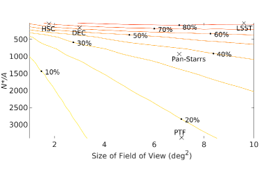
(a) The EM detection probability and optimized number of fields for a general telescope observing event 28700 (${\sim}300\,\text{deg}^{2}$).

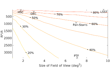
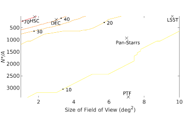
(b) The EM detection probability and optimized number of fields for a general telescope observing event 19296 (${\sim}100\,\text{deg}^{2}$).

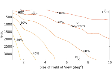
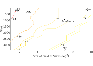
(c) The EM detection probability and optimized number of fields for a general telescope observing event 18694 (${\sim}30\,\text{deg}^{2}$).

Figure 6.— Contours of EM follow-up performance of kilonovae as a function of the size of telescope FOV and sensitivity assuming a 6 hr total observation. We show results for the 3 simulated GW events (a) event ID 28700, ${\sim}300\,\text{deg}^{2}$, (b) event ID 19296 ${\sim}100\,\text{deg}^{2}$, and event 18694 ${\sim}30\,\text{deg}^{2}$. For each event we plot contours of equal detection probability (left) and the corresponding optimal number of observing fields (right). Overlayed for reference on all plots are the locations of the telescopes considered in this work (including the proposed LSST).

V. Discussion

The behavior of the detection probability as a function of the number of observed fields (as shown in Figs. 3, 4, and 5) shows that the 2 time allocation strategies produce similar detection probabilities. In all cases the optimized approach gives marginally greater probability. As listed in Table 3 we see that for the particular cases examined in this work the fully optimal approach leads to a typical gain of a few percent in detection probability over the equal time strategy. The biggest gains of $\sim 5\%$ are obtained for the DEC telescope. These relatively modest gains suggests that spreading observation time equally is close to optimal at the optimal number of observing fields $k^{*}$. We also note that the number of fields at which the peak detection probability is achieved is similar for both strategies but always marginally lower for the equal time approach.

Both strategies clearly indicate that with a given telescope, there exits a number of fields at which the probability of a successful EM follow-up is maximized for a given GW event and a fixed amount of total observation time. In other words, exploring more or fewer fields than necessary will result in a decrease in detection probability. Although one would expect the probability of a successful EM follow-up first increases with the number of fields observed, a drop occurs if so many fields are observed that only observations of short exposure time in some or all of the observed fields are allowed, given that the observation time is fixed. This trade-off between exploring new fields and achieving increased depth within fields is broadly consistent with  Nissanke et al. (2012). Overall, for the same event, the peak detection probabilities increase as the total observation time increases. For the same telescope, the detection probability increases as the size of error region decreases. This is expected since smaller error regions mean that a telescope requires fewer fields to cover that region at a given confidence. By examining the curves in Figs. 3, 4 and 5, it can be seen that an increase in the total observation time shifts the position of the peak to larger numbers of fields, but does not change the general shape of the function.

The time allocations shown in the plots on the right of Figs. 3, 4 and 5 are those computed for the optimal number of fields. In all cases our optimal strategy ensures that proportionally more time will be assigned to those fields containing the greater fraction of GW probability (the lower index fields). In general the range in observation times per field spans $\sim 1$ order of magnitude for a given optimized observation. A surprising feature of these distributions is that the optimal time allocations can therefore differ by factors of a few per field with respect to the equal time distribution. However, both distributions result in very similar detection probabilities. Recently, Coughlin & Stubbs (2016) have produced an analytic result for the distribution of observing times under a number of simplifying assumptions including a uniform prior on peak luminosity. They recommend that the time spent per field should be proportional to the prior GW probability in each field to the $2/3$ power. We find that our numerical results are broadly consistent with this result but highlight again that the relative gains in detection probability are quite insensitive to the time allocation distribution.

Figure 6 shows our results from another perspective, namely the optimal performance of a any existing or future telescope of arbitrary sensitivity and FOV. As mentioned in Sec. II our treatment of the detection threshold criterion $N^{*}$ is simplified and hence these results should be treated as illustrative rather than definitive. However, as might be expected, a telescope with poor sensitivity and small FOV will be unlikely to detect an EM counterpart unless the GW event is particularly well localized.

That LSST should explore more fields than PTF for these GW events may seem slightly confusing at first glance as LSST’s FOV is larger than PTF’s. This is because LSST is far more sensitive than PTF and can therefore explore as many fields as needed to cover the entire error region. In comparison PTF has to spend a considerable fraction of its total observation time on each of its observed fields, which results in PTF being only able to observe a limited number of fields.

In general, the EM detection probabilities achieved are more sensitive to the telescope parameters for events with smaller error regions. For example, imagine that a telescope with a $2\,\mathrm{deg}^{2}$ FOV and a R-band limiting magnitude of $20.3$ in $30$ sec ($N^{*}/A=2273$) needed to raise the detection probability $P(D_{\mathrm{EM}}|k)$ by 10%. For event 18694, where the size of the $90\%$ credible region is ${\sim}30\,\mathrm{deg}^{2}$, it could either increase its FOV by a factor of $\approx 2$, or reduce its limiting magnitude to $\approx 21.0$ in $30$ s. However, if the $90\%$ credible region is ${\sim}300\mathrm{deg^{2}}$ as for event 28700, it would have to either further increase its FOV by a factor of $\approx 2.5$ or enhance its limiting magnitude to $\approx 21.5$ in $30$ sec to have the same factor of improvement.

In addition, the fact that at high sensitivity the contours in Fig. 6 appear to be almost flat indicates that as the size of the GW error region becomes larger, the FOV of a telescope has negligible impact on the detection probability $P(D_{EM}|\omega)$. For the design of future EM telescopes performing follow-up observations of GW events there will likely be a trade-off between sensitivity and FOV. This result implies that for GW triggers with relatively large error regions, sensitivity, rather than FOV, is the dominant factor determining EM follow-up success. However, we remind the reader that this result is based on particular choices of source and corresponding prior on the source luminosity (see Eq. 6). Different choices may have different impacts on the outcome of our method.

VI. Future Work

This work considers source sky error regions based solely on the information obtained from low latency GW sky localization (Singer & Price, 2016). One may also include galaxy catalogs to further constrain source locations within our existing Bayesian approach. In this work, the GW source distance was assumed to be statistically independent of its sky location. In the future we plan to use more realistic distance information (Singer, L. P. et al., 2016) therefore enhancing the effectiveness of our follow-up optimization strategy.

Moreover, since telescopes are distributed at various latitudes and longitudes on the Earth, different telescopes are able to see different parts of the sky at different times. As has been studied by (Rana et al., 2016) we would include the effect of observation prioritization when considering the diurnal cycle and for instances where GW sky error regions may pass below the horizon during a follow-up observation. Depending on the type of telescope considered we would also incorporate factors such as the obscuration of the source by the Sun and/or moon.

In this work, we ask the question of detecting kilonovae rather than identifying and characterizing them. The task of source identification is more demanding and will require the ability to differentiate our desired sources from contaminating backgrounds such as SNe and M-dwarf flares. One way to accomplish this is to perform multiple observations of the same fields. In this case a tentative detection is followed by an observation of the candidate for a period of time until the source’s light curve allows it to be classify as a kilonova or contaminating noise (Cowperthwaite & Berger, 2015; Nissanke et al., 2012). As mentioned in Sec. II, simply repeating our proposed observations would enable the identification of variable objects for deeper follow-ups. However, a more involved procedure could incorporate light-curve information into our strategy therefore jointly optimizing the pointings used in both the detection and identification stages. This more complex strategy is left for future implementation.

VII. Conclusion

In summary, we have demonstrated a proof-of-concept method for quantifying and maximizing the probability of a successful EM follow-up of a candidate GW event. We have applied this method to kilonovae counterparts but we emphasize that this method is versatile and applicable to any EM counterpart model. We have shown that there exists an optimal number of fields on which time should be spent, and that observing more or fewer fields will result in a decrease in the detection probability. This analysis has been based on the assumptions of a static telescope with unconstrained pointings, a kilonova source at constant peak luminosity and the independence of statistical uncertainty between the distance and the GW trigger sky location.

Our approach takes as inputs the GW sky localization information, and the selected telescope’s characteristics. The method selects the observed field locations with a greedy algorithm and then uses Lagrange Multipliers to compute the time allocation for those fields based on maximizing the detection probability. We have tested the algorithm by optimizing the EM follow-up observations of the HSC, DEC, Pan-Starrs, and PTF telescopes for three simulated GW events. By comparing the results of our methods with the results of equally dividing the observation time amongst the observed fields, we have shown that both strategies return similar results, with our method producing marginally larger detection probabilities.

In addition, we have provided estimates for the EM follow-up performance of a general telescope of arbitrary sensitivity and FOV. These results indicate that in terms of telescope design, the likelihood of its success in the follow-up of kilonova signals is approximately independent of the FOV for reasonably sensitive telescopes.

To extend this work, it may be helpful to consider including constraints from galaxy catalogs on source location. Also, the assumptions that the kilonova luminosity is constant during the observation period, more realistic treatment of the source distance, and consideration of the dynamics of the telescope with respect to the source should also be investigated. Finally, the inclusion of multiple observations of the same fields should be implemented to help distinguish kilonovae from contaminating sources.

References

- Abbott et al. (2016a) Abbott, B. et al. 2016a, Physical review letters, 116, 061102
- Abbott et al. (2016b) Abbott, B. P. et al. 2016b, Phys. Rev. Lett., 116, 241103
- Abell et al. (2009) Abell, P. A., Allison, J., Anderson, S. F., Andrew, J. R., Angel, J. R. P., Armus, L., Arnett, D., Asztalos, S., Axelrod, T. S., Bailey, S., et al. 2009, arXiv preprint arXiv:0912.0201
- Barnes & Kasen (2013) Barnes, J. & Kasen, D. 2013, The Astrophysical Journal, 775, 18
- Bartos et al. (2015a) Bartos, I., Crotts, A. P. S., & Márka, S. 2015a, The Astrophysical Journal Letters, 801, L1
- Bartos et al. (2015b) Bartos, I., Huard, T., & Marka, S. 2015b, in prep.
- Berger et al. (2013) Berger, E., Fong, W., & Chornock, R. 2013, The Astrophysical Journal, 774, L23
- Bernstein et al. (2012) Bernstein, J., Kessler, R., Kuhlmann, S., Biswas, R., Kovacs, E., Aldering, G., Grane, I., D’Andrea, C., Finley, D., Frieman, J., et al. 2012, The Astrophysical Journal, 152
- Blackburn et al. (2015) Blackburn, L., Briggs, M. S., Camp, J., Christensen, N., Connaughton, V., Jenke, P., Remillard, R. A., & Veitch, J. 2015, The Astrophysical Journal Supplement Series, 217, 8
- Bloom et al. (2009) Bloom, J. S., Holz, D. E., Hughes, S. A., & Menou, K. 2009, 2010
- Coughlin & Stubbs (2016) Coughlin, M. W. & Stubbs, C. W. 2016, arXiv preprint arXiv:1604.05205
- Cowperthwaite & Berger (2015) Cowperthwaite, P. S. & Berger, E. 2015, The Astrophysical Journal, 814, 25
- Fan et al. (2014) Fan, X., Messenger, C., & Heng, I. S. 2014, The Astrophysical Journal, 795, 43
- Gehrels et al. (2016) Gehrels, N., Cannizzo, J. K., Kanner, J., Kasliwal, M. M., Nissanke, S., & Singer, L. P. 2016, The Astrophysical Journal, 820, 136
- Grossman et al. (2014) Grossman, D., Korobkin, O., Rosswog, S., & Piran, T. 2014, Monthly Notices of the Royal Astronomical Society, 439, 757
- Jin et al. (2016) Jin, Z.-P., Hotokezaka, K., Li, X., Tanaka, M., D’Avanzo, P., Fan, Y.-Z., Covino, S., Wei, D.-M., & Piran, T. 2016, arXiv preprint arXiv:1603.07869
- Jin et al. (2015) Jin, Z.-P., Li, X., Cano, Z., Covino, S., Fan, Y.-Z., & Wei, D.-M. 2015, The Astrophysical Journal Letters, 811, L22
- Kaiser et al. (2002) Kaiser, N., Aussel, H., Burke, B. E., Boesgaard, H., Chambers, K., Chun, M. R., Heasley, J. N., Hodapp, K.-W., Hunt, B., Jedicke, R., Jewitt, D., Kudritzki, R., Luppino, G. A., Maberry, M., Magnier, E., Monet, D. G., Onaka, P. M., Pickles, A. J., Rhoads, P. H. H., Simon, T., Szalay, A., Szapudi, I., Tholen, D. J., Tonry, J. L., Waterson, M., & Wick, J. 2002, Survey and Other Telescope Technologies and Discoveries. Edited by Tyson, 4836, 154
- Kulkarni & Kasliwal (2009) Kulkarni, S. & Kasliwal, M. M. 2009, 312
- Law et al. (2009) Law, N. M., Kulkarni, S. R., Dekany, R. G., Ofek, E. O., Quimby, R. M., Nugent, P. E., Surace, J., Grillmair, C. C., Bloom, J. S., Kasliwal, M. M., et al. 2009, Publications of the Astronomical Society of the Pacific, 121, 1395
- Li & Paczynski (1998) Li, L.-X. & Paczynski, B. 1998, The Astrophysical Journal Letters, 507, L59
- Li et al. (2016) Li, X., Hu, Y.-M., Fan, Y.-Z., & Wei, D.-M. 2016, arXiv.org, arXiv:1601.00180
- Metzger et al. (2015) Metzger, B. D., Bauswein, A., Goriely, S., & Kasen, D. 2015, MNRAS, 446, 1115
- Metzger & Berger (2011) Metzger, B. D. & Berger, E. 2011, The Astrophysical Journal, 746, 16
- Miyazaki et al. (2012) Miyazaki, S., Komiyama, Y., Nakaya, H., Kamata, Y., Doi, Y., Hamana, T., Karoji, H., Furusawa, H., Kawanomoto, S., Morokuma, T., et al. 2012, in SPIE Astronomical Telescopes+ Instrumentation, International Society for Optics and Photonics, 84460Z–84460Z
- Nissanke et al. (2012) Nissanke, S., Kasliwal, M., & Georgieva, A. 2012, The Astrophysical Journal, 124, 124
- Phinney (2009) Phinney, E. S. 2009, 2010
- Rana et al. (2016) Rana, J., Singhal, A., Gadre, B., Bhalerao, V., & Bose, S. 2016, arXiv preprint arXiv:1603.01689
- Singer et al. (2016) Singer, L., Chen, H.-Y., Holz, D. E., Farr, W. M., Price, L. R., Raymond, V., Cenko, S. B., Gehrels, N., Cannizzo, J., Kasliwal, M. M., et al. 2016, arXiv preprint arXiv:1605.04242
- Singer et al. (2012) Singer, L., Price, L., & Speranza, A. 2012, arXiv preprint arXiv:1204.4510
- Singer & Price (2016) Singer, L. P. & Price, L. R. 2016, Physical Review D, 93, 024013
- Singer et al. (2014) Singer, L. P., Price, L. R., Farr, B., Urban, A. L., Pankow, C., Vitale, S., Veitch, J., Farr, W. M., Hanna, C., Cannon, K., Downes, T., Graff, P., Haster, C.-J., Mandel, I., Sidery, T., & Vecchio, A. 2014, The Astrophysical Journal, 795, 105
- Singer, L. P. et al. (2016) Singer, L. P., Chen, H. Y., Holz, D. E., Farr, W. M., Price, L. R., Raymond, V., Cenko, S. B., Gehrels, N., Cannizzo, J., Kasliwal, M. M., Nissanke, S., Coughlin, M., Farr, B., Urban, A. L., Vitale, S., Veitch, J., Graff, P., Berry, C. P. L., Mohapatra, S., & Mandel, I. 2016, arXiv.org, arXiv:1603.07333
- Tanaka et al. (2014) Tanaka, M., Hotokezaka, K., Kyutoku, K., Wanajo, S., Kiuchi, K., Sekiguchi, Y., & Shibata, M. 2014, The Astrophysical Journal, 780, 31
- Tanvir et al. (2013) Tanvir, N. R., Levan, a. J., Fruchter, a. S., Hjorth, J., Hounsell, R. a., Wiersema, K., & Tunnicliffe, R. L. 2013, Nature, 500, 547
- Veitch et al. (2015) Veitch, J., Raymond, V., Farr, B., Farr, W., Graff, P., Vitale, S., Aylott, B., Blackburn, K., Christensen, N., Coughlin, M., Del Pozzo, W., Feroz, F., Gair, J., Haster, C.-J., Kalogera, V., Littenberg, T., Mandel, I., O’Shaughnessy, R., Pitkin, M., Rodriguez, C., Röver, C., Sidery, T., Smith, R., Van Der Sluys, M., Vecchio, A., Vousden, W., & Wade, L. 2015, Physical Review D, 91, 042003
- Yang et al. (2015) Yang, B., Jin, Z.-P., Li, X., Covino, S., Zheng, X.-Z., Hotokezaka, K., Fan, Y.-Z., Piran, T., & Wei, D.-M. 2015, NATURE COMMUNICATIONS, 6, 7323