Defining Coherent Vortices Objectively from the Vorticity

Abstract

Rotationally coherent Lagrangian vortices are formed by tubes of deforming fluid elements that complete equal bulk material rotation relative to the mean rotation of the deforming fluid volume. We show that initial positions of such tubes coincide with tubular level surfaces of the Lagrangian-Averaged Vorticity Deviation (LAVD), the trajectory integral of the normed difference of the vorticity from its spatial mean. LAVD-based vortices are objective, i.e., remain unchanged under time-dependent rotations and translations of the coordinate frame. In the limit of vanishing Rossby numbers in geostrophic flows, cyclonic LAVD vortex centers are precisely the observed attractors for light particles. A similar result holds for heavy particles in anticyclonic LAVD vortices. We also establish a relationship between rotationally coherent Lagrangian vortices and their instantaneous Eulerian counterparts. The latter are formed by tubular surfaces of equal material rotation rate, objectively measured by the Instantaneous Vorticity Deviation (IVD). We illustrate the use of the LAVD and the IVD to detect rotationally coherent Lagrangian and Eulerian vortices objectively in several two- and three-dimensional flows.

1 Introduction

Coherent vortices still have no universal definition in fluid mechanics, but two main features of a possible definition have been emerging. First, vortices are broadly agreed to be concentrated regions of high vorticity. Some authors require this dominance of vorticity relative to other flow domains (McWilliams 1984, Hussein 1986), others expect it relative to the strain in the same domain (Okubo 1970, Hunt et al. 1988, Weiss 1991, Hua & Klein 1998, Hua, McWilliams & Klein 1998). Yet others compare vorticity to strain in the rate-of-strain eigenbasis (Tabor & Klapper 1995; see also Lapeyre, Klein & Hua 1999, and Lapeyre, Hua & Legras 2001).

Second, vortices are generally viewed as evolving domains with a high degree of material invariance. Lugt (1979) writes that a vortex is a “multitude of material particles rotating around a common center”. McWilliams (1984) expects the vortex to “persist under passive advection by the large-scale flow”. Chong, Perry & Cantwell (1990) propose to capture vortices by finding spiraling particle motions in the frozen-time limit of the flow. Vortices are described as “highly impermeable to inward and outward particle fluxes” by Provenzale (1999), who requires small relative dispersion within vortex cores (see also Cucitore Quadrio & Baron 1999). Chakraborty, Balachandar & Adrian (2005) proposes that both swirling motion and small particle separation should be distinguishing features of a vortex core. Haller (2005) views vortices as sets of trajectories with a persistent lack of Lagrangian hyperbolicity. Chelton et al. (2011) observe that nonlinear eddies (vortices with a rotation speed exceeding their translation speed) trap fluid in their interior and transport them along. Finally, in a similar geophysical setting, Mason, Pascual & McWilliams (2014) stress that vortices are “efficient carriers of mass and its physical, chemical, and biological properties”.

The core of a coherent vortex is, therefore, broadly expected to be an impermeable material region marked by a high concentration of vorticity. What constitutes high vorticity is, however, subject to individual judgement, thresholding, and choice of the reference frame. It is therefore the material invariance of a vortex core that holds more promise as a first requirement in an unambiguous vortex definition. Indeed, the Lagrangian nature of a vortex can simply be assured by defining its boundary as a tubular (i.e., cylindrical, cup-shaped or toroidal) material surface. The challenging next step is then to select such a material surface in a way that it also encloses a region of concentrated vorticity.

Unlike vorticity, materially defined vortex boundary surfaces are inherently frame-invariant, defined by a set of fluid trajectories rather than by coordinates or instantaneous scalar field values. In continuum mechanics terminology, a material vortex boundary must therefore be objective, i.e., invariant with respect to all Euclidean frame changes of the form

$$x=Q(t)y+b(t),$$ (1)

where $x\in\mathbb{R}^{3}$ and $y\in\mathbb{R}^{3}$ denote coordinates in the original and in the transformed frame, respectively; $Q(t)\in SO(3)$ is an arbitrary rotation matrix; and $b(t)\in\mathbb{R}^{3}$ is an arbitrary translation vector (Truesdell & Noll 1965). Paradoxically, with the exception of the approach initiated by Tabor & Klapper (1995), none of the instantaneous Eulerian vortex criteria listed above are objective. Accordingly, they may only detect coherent structures after passage to an appropriately rotating or translating coordinate frame. For instance, the unsteady Navier-Stokes velocity field

$$v(x,t)=\left(\begin{array}[]{c}x_{1}\sin 4t+x_{2}(2+\cos 4t)\\ x_{1}(\cos 4t-2)-x_{2}\sin 4t\\ 0\end{array}\right),$$ (2)

is classified as a vortex by the Okubo–Weiss, Hua–Klein, Hua–McWilliams–Klein, and Chakraborty–Balachandar–Adrian criteria, as well as by the $Q$-criterion of Hunt et al., the $\Delta$-criterion of Chong, Perry and Cantwell, and the nonlinear eddy criterion of Chelton et al. In reality, (2) is a rotating saddle-point flow, with typical trajectories growing exponentially in norm. This instability, however, only becomes detectable to these criteria after one passes to an appropriately chosen rotating frame (Haller 2005, 2015). Promisingly, if we simply impose the localized high-vorticity requirement, the constant-vorticity flow (2) is immediately discounted as a vortex without further need for analysis.

Selecting vortex boundaries as material surfaces ensures material invariance for the vortex, but any tubular material surface can a priori be considered for this purpose. Recent stretching-based variational approaches narrow down this consideration to exceptional material tubes that remain perfectly unfilamented under material advection (Haller & Beron–Vera 2013, Blazevski & Haller 2004, Haller 2015). As an alternative, Farazmand & Haller (2016) seek vortex boundaries as maximal material tubes along which material elements complete the same polar rotation over a finite time interval of interest. These approaches have proven effective in two-dimensional flows. They, however, rely on a precise computation of the invariants of the Cauchy–Green strain tensor along a Lagrangian grid, which requires the accurate numerical differentiation of trajectories with respect to their initial positions. This presents a challenge in three-dimensional unsteady flows, for which the polar rotation approach additionally fails to be objective. Most importantly, however, Lagrangian strain-based approaches offer no link between material vortices and the expected high vorticity concentration, a defining feature of observed vortices.

In summary, despite recent advances in vortex criteria and fluid trajectory stability analysis, a fully three-dimensional, computationally tractable and objective global vortex definition, with guaranteed material invariance and experimentally observable rotational coherence, has not yet emerged. Here we propose such a vortex definition and a corresponding vortex detection technique.

Our approach is based on a recently obtained, unique decomposition of the deformation gradient into the product the two deformation gradients: one for a purely straining flow and one for a purely rotational flow (Haller 2016). This rotational deformation gradient, the dynamic rotation tensor, obeys the temporal superposition property of rigid body rotations, thereby eliminating a dynamical inconsistency of the classic polar rotation tensor used in classical continuum mechanics. The dynamic rotation tensor can further be factorized into a spatial mean-rotation component and a deviation from this rotation. The latter deviatory part yields an objective, intrinsic material rotational angle relative to the deforming fluid mass.

We then define a rotationally coherent Lagrangian vortex as a nested set of material tubes, each exhibiting uniform intrinsic material rotation. Such a vortex turns out to be foliated by outward decreasing tubular level sets of the Lagrangian-averaged vorticity (LAVD). Additionally, we prove that the center of an LAVD-based vortex is always the observed attractor for nearby finite-size (inertial) particle motions in geostrophic flows.

In the limit of zero advection time, our Lagrangian vortex definition turns into an objective Eulerian vortex definition: a set of tubular surfaces of equal intrinsic rotation rate. These surfaces are tubular level sets of the instantaneous vorticity deviation (IVD), providing a mathematical link between rotationally coherent Eulerian and Lagrangian vortices: the former are effectively derivatives of the latter. We illustrate our results on several examples, ranging from analytic velocity fields to time-dependent two- and three-dimensional models and observational data.

2 Set-up

We consider an unsteady velocity field $v(x,t)$, defined on a possibly time-dependent spatial domain $U(t)\subset\mathbf{\mathbb{R}}^{3}$ over a finite time interval $[t_{0},t_{1}].$ We assume that $U(t)$ is invariant under the fluid flow generated by the velocity field (cf. eq. (8) below). Thus, $U(t)$ is either a physical domain with an impermeable boundary, or $U(t)$ is a material domain formed by a set of evolving trajectories of $v(x,t)$.

We write the velocity gradient $\nabla v$ as

$$\nabla v(x,t)=D(x,t)+W(x,t),$$ (3)

where $D=\frac{1}{2}\left(\nabla v+\left[\nabla v\right]^{T}\right)$ is the rate of stain tensor and $W=\frac{1}{2}\left(\nabla v-\left[\nabla v\right]^{T}\right)$ is the spin tensor. We recall that the vorticity $\omega=\nabla\times v$ of the fluid satisfies

$$We=-\frac{1}{2}\omega\times e,\qquad\forall e\in\mathbb{R}^{3}.$$ (4)

We will also use the instantaneous spatial mean $\bar{\omega}$ of the vorticity over $U(t)$, defined as

$$\bar{\omega}(t)=\frac{\int_{U(t)}\omega(x,t)\,dV}{\mathrm{vol}\,(U(t))},$$ (5)

where $\mathrm{vol}\,(\cdot\,)$ denotes the volume for three-dimensional flows, and the area for two-dimensional flows. Accordingly, $dV$ refers to the volume or area element, respectively, in $U(t)$.

Under general observer changes of the form (1), the spin tensor and the vorticity in the new $y$ coordinate frame take the form

$$\tilde{W}(y,t)=Q^{T}(t)W(x,t)Q(t)-Q^{T}(t)\dot{Q}(t),\qquad\tilde{\omega}(y,t)=Q^{T}(t)\omega(x,t)+\dot{q}(t),$$ (6)

with the vector $\dot{q}$ defined uniquely by the relation $\dot{Q}Q^{T}e=\frac{1}{2}\dot{q}\times e$ for all $e\in\mathbb{R}^{3}$ (see, e.g., Truesdell & Rajagopal 2009). Formula (6) shows that the spin tensor and the vorticity are not objective quantities: the eigenvalues and eigenvectors of $W$ change in rotating frames, and so does the direction and the magnitude of $\omega$. Thus, neither $W$ nor $\omega$ is, by itself, suitable for defining distinguished material sets in the flow. This is because material sets are tied to evolving fluid particles without any reference to coordinates, and hence are inherently frame-invariant. More generally statements about the material response of a moving continuum cannot depend on the observer and hence should be objective (Gurtin 1982).

Fluid particle trajectories generated by $v(x,t)$ are solutions of the differential equation

$$\dot{x}=v(x,t),$$

defining the flow map

$$\mathcal{F}_{t_{0}}^{t}\colon x_{0}\mapsto x(t;x_{0}),\qquad\ t\in[t_{0},t_{1}],$$ (7)

as the mapping from initial particle positions $x_{0}\in U(t_{0})$ to their later positions $x(t;x_{0})\in U(t)$. The assumed invariance of $U(t)$ over the time interval $[t_{0},t_{1}]$ can now be conveniently expressed as

$$\mathcal{F}_{t_{0}}^{t}(U(t_{0}))=U(t)\qquad t\in[t_{0},t_{1}].$$ (8)

We will also use the notion of a material surface, which is a smooth, codimension-one, time-dependent surface family $\mathcal{M}(t)$ advected by the flow, i.e., $\mathcal{M}(t)=\mathcal{F}_{t_{0}}^{t}(\mathcal{M}(t_{0}))\qquad t\in[t_{0},t_{1}].$

The deformation gradient

$$F_{t_{0}}^{t}(x_{0})=\nabla\mathcal{F}_{t_{0}}^{t}(x_{0})$$ (9)

is a linear map, taking initial infinitesimal perturbations to the fluid trajectory $x(t;x_{0})$ at time $t_{0}$ to their later positions at time $t$. Although often believed otherwise, $F_{t_{0}}^{t}$ is not objective: its eigenvectors and eigenvalues depend on the frame of reference (see, e.g., Liu 2004). Therefore, the invariants of $F_{t_{0}}^{t}$ do not provide an objective indication of the rotational component of the deformation.

3 Finite material rotation from the Dynamic Polar Decomposition

We seek to identify coherent Lagrangian vortices as the union of tubular material surfaces in which fluid elements exhibit the same bulk material rotation over a finite time interval of interest. Individual material fibers based at an initial point $x_{0}$ in a deforming continuum, however, all rotate around different axes and by different angles. In recent work (Farazmand & Haller 2016), we used the classic polar rotation angle (PRA) from finite strain theory to identify pointwise bulk material rotation in a moving fluid systematically. The use of the PRA, however, also leaves several challenges unaddressed, as we discuss in Appendix A. Most notable of these are an inconsistency of the PRA with experimentally observed dynamic rotation angles of spherical tracers in fluids, and its lack of objectivity in three dimensions.

To address these challenges, we use here the recently developed Dynamic Polar Decomposition (DPD) to identify a dynamically consistent and fully frame-invariant rotational component in the finite deformation of fluid elements (Haller 2016). This decomposition gives a unique, time-evolving factorization of the deformation gradient into the product of two deformation gradients: one for a purely rotational flow with zero rate of strain, and one for a purely straining flow with zero vorticity.

Specifically, the unique right DPD of $F_{t_{0}}^{t}$ at $x_{0}$ can be written as

$$F_{t_{0}}^{t}=O_{t_{0}}^{t}M_{t_{0}}^{t},\qquad t\in[t_{0},t_{1}],$$ (10)

where the proper orthogonal dynamic rotation tensor $O_{t_{0}}^{t}=\partial_{a_{0}}a(t)$ is the deformation gradient of the purely rotational flow

$$\dot{a}=W\left(x(t;x_{0}),t\right)a,$$ (11)

and the non-degenerate right dynamic stretch tensor $M_{t_{0}}^{t}=\partial_{b_{0}}b(t)$ is the deformation gradient of the purely straining flow

$$\dot{b}=O_{t}^{t_{0}}D\left(x(t;x_{0}),t\right)O_{t_{0}}^{t}b.$$ (12)

The linear velocity field for $a(t)$ in (11) is strainless because its coefficient matrix $W$ is skew-symmetric. Similarly, the linear velocity field for $b(t)$ in (12) is irrotational because its coefficient matrix $O_{t}^{t_{0}}D\left(x(t;x_{0}),t\right)O_{t_{0}}^{t}$ is symmetric. Unlike the classic polar rotation tensor (cf. Appendix A), the dynamic rotation tensor $O_{t_{0}}^{t}$ is dynamically consistent, i.e., satisfies the fundamental superposition property of solid-body rotations:

$$O_{t_{0}}^{t}=O_{s}^{t}O_{t_{0}}^{s},\qquad s,t\in[t_{0},t_{1}].$$ (13)

This follows because $O_{t_{0}}^{t}$ is the fundamental matrix solution of a classical linear differential equation and hence satisfies the process property noted in (13) (cf. Dafermos 1971, Arnold 1978). In contrast, $M_{t_{0}}^{t}$ is the fundamental matrix solution of a non-classical linear differential equation with memory, i.e., with explicit dependence on the initial time $t_{0}$. Such fundamental solutions do not obey the process-property indicated in (13). The reason behind the dynamical inconsistency (35) of polar rotations is a similar memory effect in eq. (34).

The decomposition in (10) is a right-type decomposition, i.e., the dynamic stretch tensor precedes the dynamic rotation tensor from the right. Just as for the classic polar decomposition, a left-type version of the DPD is also available (Haller 2016).

4 Lagrangian-averaged vorticity deviation (LAVD)

Despite its dynamical consistency, the dynamic rotation tensor $O_{t_{0}}^{t}$ is not objective. Its frame-dependence is the consequence of the frame-dependence of the spin tensor $W(x,t)$ appearing in the differential equation (11). The single remaining challenge out of those listed in Appendix A is, therefore, to identify an objective part of the rotation described by $O_{t_{0}}^{t}$ which also preserves the dynamical consistency of $O_{t_{0}}^{t}$. Below we recall further results from Haller (2016), and use them to address this challenge.

The dynamic rotation tensor $O_{t_{0}}^{t}$ can further be factorized into two deformation gradients: one for a spatially uniformly rotating flow, and one for a flow that describes deviations from this uniform rotation. Specifically, we have

$$O_{t_{0}}^{t}=\Phi_{t_{0}}^{t}\Theta_{t_{0}}^{t},$$ (14)

where the proper orthogonal relative rotation tensor $\Phi_{t_{0}}^{t}=\partial_{\alpha_{0}}\alpha(t)$ is dynamically consistent, serving as the deformation gradient of the relative rotation flow

$$\dot{\alpha}=\left[W\left(x(t;x_{0}),t\right)-\bar{W}\left(t\right)\right]\alpha.$$ (15)

In contrast, the proper orthogonal mean rotation tensor $\Theta_{t_{0}}^{t}=D_{\beta_{0}}\beta(t)$ is the deformation gradient of the mean-rotation flow

$$\dot{\beta}=\Phi_{t}^{t_{0}}\bar{W}\left(t\right)\Phi_{t_{0}}^{t}\beta.$$ (16)

The mean rotation tensor $\Theta_{t_{0}}^{t}$ is not dynamically consistent because (16) exhibits the same memory effect discussed for (12).

The dynamic consistency of $\Phi_{t_{0}}^{t}$ implies that the total angle swept by this tensor around its own axis of rotation is dynamically consistent. This angle $\psi_{t_{0}}^{t}(x_{0})$, called intrinsic rotation angle (see Fig. (1)), therefore satisfies

$$\psi_{t_{0}}^{t}(x_{0})=\psi_{s}^{t}(x_{0})+\psi_{t_{0}}^{s}(x_{0}),\qquad s,t\in[t_{0},t_{1}].$$

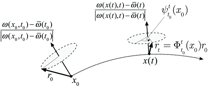
Figure 1: The geometry of the intrinsic rotation angle $\psi_{t_{0}}^{t}(x_{0})$ along a material trajectory $x(t)$ in a three-dimensional deforming continuum.

In addition, as shown in Haller (2016), $\psi_{t_{0}}^{t}(x_{0})$ is objective both in two and three dimensions. In two dimensions, even the tensor $\Phi_{t_{0}}^{t}$ itself turns out to be objective, not just its associated scalar field $\psi_{t_{0}}^{t}(x_{0})$.

Using the results obtained in Haller (2016), the intrinsic dynamic rotation $\psi_{t_{0}}^{t}(x_{0})$ can be computed as

$$\psi_{t_{0}}^{t}(x_{0})=\frac{1}{2}\mathrm{LAVD}_{t_{0}}^{t}(x_{0}),$$ (17)

with the Lagrangian-Averaged Vorticity Deviation (LAVD) defined here as

$$\mathrm{LAVD}_{t_{0}}^{t}(x_{0}):=\int_{t_{0}}^{t}\left|\omega(x(s;x_{0}),s)-\bar{\omega}(s)\right|\,ds.$$ (18)

The objectivity of $\psi_{t_{0}}^{t}$ and LAVD can be confirmed directly from formula (6). Indeed, under a Euclidean observer change $x=Q(t)y+b(t)$, the transformed vorticity $\tilde{\omega}(y,t)$ satisfies

$$\left|\tilde{\omega}(y(s),s)-\tilde{\bar{\omega}}(s)\right| = \left|Q^{T}(s)\omega(x(s),s)+Q^{T}(t)\dot{q}(t)-\left(Q^{T}(s)\bar{\omega}(s)+Q^{T}(t)\dot{q}(t)\right)\right|$$ (19)

$$= \left|Q^{T}(s)\left[\omega(x(s),s)-\bar{\omega}(s)\right]\right|$$

$$= \left|\omega(x(s),s)-\bar{\omega}(s)\right|,$$

because the rotation matrix $Q^{T}(s)$ preserves the length of vectors. We summarize the results of this section in a theorem.

Theorem 1.

For an infinitesimal fluid volume starting from $x_{0}$, the $\mathrm{LAVD}_{t_{0}}^{t}(x_{0})$ field is a dynamically consistent and objective measure of bulk material rotation relative to the spatial mean-rotation of the fluid volume $U(t)$. Specifically, $\mathrm{LAVD}_{t_{0}}^{t}(x_{0})$ is twice the intrinsic dynamic rotation angle generated by the relative rotation tensor $\Phi_{t_{0}}^{t}$. The latter tensor is obtained from the dynamically consistent decomposition

$$F_{t_{0}}^{t}=\Phi_{t_{0}}^{t}\Theta_{t_{0}}^{t}M_{t_{0}}^{t}$$ (20)

with the deformation gradient $\Theta_{t_{0}}^{t}$ of a pure rigid-body rotation, and with the deformation gradient $M_{t_{0}}^{t}$of a unique, purely straining flow.

For detailed proofs of all statements in Theorem 1, we refer the reader to Haller (2016). Importantly, this theorem enables the extraction of an objective and dynamically consistent, material rotation component from the deformation gradient without carrying out the differentiation with respect to initial conditions in the definition (9) of $F_{t_{0}}^{t}$.

5 Rotationally coherent Lagrangian vortices

We now use the LAVD to identify objectively material tubes along which small fluid volumes experience the same bulk rotation over $[t_{0},t_{1}]$ relative to the mean rigid-body rotation of the fluid. By Theorem 1, the time $t_{0}$ positions of such material tubes are tubular level surfaces of the scalar function $\mathrm{LAVD}_{t_{0}}^{t_{1}}(x_{0})$. By a tubular set, we mean here a convex, cylindrical, cup-shaped or toroidal set in three dimensions, and a closed convex curve in two dimensions. We require convexity for tubular surfaces, motivated by the near-circular cross section generally observed for stable vortices.

If the gradient $\partial_{x_{0}}\mathrm{LAVD}_{t_{0}}^{t_{1}}(x_{0})$ is nonzero along a tubular LAVD level surface, then this level surface is surrounded by a continuous, nested family of tubular level surfaces (Milnor 1963). The singular center of such a nested sequence of tubes, with inward increasing LAVD values, gives a definition of a Lagrangian vortex center. Similarly, the largest convex member of such a nested tube family defines the boundary of a Lagrangian vortex. We summarize these concepts in the following definition, with its geometry illustrated in Fig. 2.

Definition 1.

Over the finite time interval $[t_{0},t_{1}]$:

(i) A rotationally coherent Lagrangian vortex is an evolving material domain $\mathcal{V}(t)$ such that $\mathcal{V}(t_{0})$ is filled with a nested family of tubular level surfaces of $\mathrm{LAVD}_{t_{0}}^{t_{1}}(x_{0})$ with outward-decreasing LAVD values.

(ii) The boundary $\mathcal{B}(t)$ of $\mathcal{V}(t)$ is a material surface such that $\mathcal{B}(t_{0})$ is the outermost tubular level surface of $\mathrm{LAVD}_{t_{0}}^{t_{1}}(x_{0})$ in $\mathcal{V}(t_{0})$.

(iii) The center $\mathcal{C}(t)$ of $\mathcal{V}(t)$ is a material set $\mathcal{C}(t)$ such that $\mathcal{C}(t_{0})$ is the innermost member (maximum) of the $\mathrm{LAVD}_{t_{0}}^{t_{1}}(x_{0})$ level-surface family in $\mathcal{V}(t_{0})$.

We refer to the evolving positions $\mathcal{L}(t)$ of the tubular level sets

$$\mathcal{L}(t_{0})=\left\{x_{0}\in U(t_{0})\,:\,\mathrm{LAVD}_{t_{0}}^{t_{1}}(x_{0})=const.\right\}$$

as a rotational Lagrangian Coherent Structure (rotational LCS), as indicated in Fig. 2. These LCSs give a foliation of the evolving Lagrangian vortex $\mathcal{V}(t)$ into tubes along which material elements complete the same intrinsic dynamic rotation $\psi_{t_{0}}^{t}(x_{0})$.

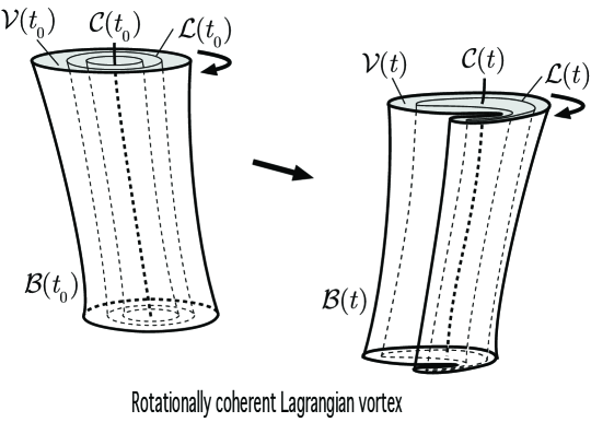
Figure 2: Initial and current positions of a rotationally coherent Lagrangian vortex $\mathcal{V}(t)$; a Lagrangian vortex boundary $\mathcal{B}(t);$ and a Lagrangian vortex center $\mathcal{C}(t)$. Also shown within $\mathcal{V}(t)$ is a rotational LCS $\mathcal{L}(t)$, i.e., a material surface along which volume elements exhibit the same intrinsic dynamic rotation over the time interval $[t_{0},t_{1}].$ As a consequence, $\mathcal{V}(t)$ experiences only tangential material filamentation without global breakaway.

Rotational LCSs, as well as Lagrangian vortices, their boundaries and centers are material objects by definition. Therefore, their time $t$ position is uniquely determined by Lagrangian advection of their initial positions:

$$\mathcal{L}(t)=\mathcal{F}_{t_{0}}^{t}\left(\mathcal{L}(t_{0})\right),\qquad\mathcal{B}(t)=\mathcal{F}_{t_{0}}^{t}\left(\mathcal{B}(t_{0})\right),\qquad\mathcal{C}(t)=\mathcal{F}_{t_{0}}^{t}\left(\mathcal{C}(t_{0})\right),\qquad t\in[t_{0},t_{1}].$$

Recent stretching-based definitions of Lagrangian vortices allow for no filamentation in boundary of the vortex (Haller & Beron–Vera 2013, Blazevski & Haller 2014). In contrast, the LAVD-based definition of a rotational LCS allows for tangential material filamentation. The filamented part of the material surface, however, still rotates together with the LCS without global breakaway.

The above definitions capture Lagrangian vortices with the simplest (i.e., convex) geometry at time $t_{0}$. More generally, one may allow for small tangential filamentation to be a priori present in the vortex boundary even at time $t_{0}$. This involves the relaxation of the convexity of $\mathcal{L}(t_{0})$ and $\mathcal{B}(t_{0})$ to material surfaces with small convexity deficiency, as discussed along with other numerical aspects in Section 9.

In geophysical flows over a rotating planet, rotationally coherent Lagrangian vortices can directly be computed from the flow induced in the curvilinear coordinate space instead of the curved surface of the planet (cf. Appendix B). By construction, the resulting vortices and their centers are invariant with respect to time-dependent rotations and translations within the space of curvilinear coordinates. With this approach, one simply computes the classic Euclidean vorticity of the longitudinal and latitudinal coordinate speeds, as opposed to computing the vorticity in curvilinear coordinates.

6 Rotationally coherent Eulerian vortices

Over a short time interval $[t_{0},t+s]$ with $\left|s\right|\ll 1$, we can Taylor expand the LAVD field as

$$\mathrm{LAVD}_{t_{0}}^{t+s}(x_{0})=\mathrm{LAVD}_{t_{0}}^{t}(x_{0})+\mathrm{IVD}(x(t;x_{0}),t)\cdot s+\mathcal{O}\left(s^{2}\right),$$ (21)

with the instantaneous vorticity deviation (IVD) defined as

$$\mathrm{IVD}(x,t):=\left|\omega(x,t)-\bar{\omega}(t)\right|.$$ (22)

By the calculation (19), the IVD field is objective. By equation (21), $\mathrm{IVD}(x(t;x_{0}),t)$ describes the rate of change of the LAVD field at an initial condition $x_{0}$ under increasing integration time.

Using the IVD, we now introduce the instantaneous notion of a rotationally coherent Eulerian vortex by taking the limit $t_{0},t_{1}\to t$ in Definition 1. At a time $t\in[t{}_{0},t_{1}],$ such an Eulerian vortex is composed of tubular surfaces along which the intrinsic rotation rates $\dot{\psi}_{t}^{t}$ of fluid elements are equal. Indeed, by formula (17), we have $\dot{\psi}_{t}^{t}(x)=\frac{1}{2}\mathrm{IVD}(x,t)=const.$ along these tubular surfaces. The following definition summarizes the details for this objective Eulerian vortex concept.

Definition 2.

At a time instance $t\in[t_{0},t_{1}]:$

(i) A rotationally coherent Eulerian vortex is a set $V(t)$ filled with a nested family of tubular level sets of $IVD(x,t)$ with outwards non-increasing IVD values.

(ii) The boundary $B(t)$ of $V(t)$ is the outermost level surface of $\mathrm{IVD}(x,t)$ in $V(t)$.

(iii) The center $C(t)$ of $V(t)$ is the innermost member (maximum) of the $\mathrm{IVD}(x,t)$ level-surface family in $V(t)$.

A rotational Eulerian Coherent Structure (rotational ECS) is then just a level surface

$$E(t)=\left\{x\in U(t)\,:\,\mathrm{IVD}(x,t)=C_{0}(t)\right\}$$ (23)

along which material elements experience the same dynamic rotation rate $\dot{\psi}_{t}^{t}(x)=C_{0}(t)/2$. Unlike rotational LCSs, individual rotational ECSs are instantaneous quantitates without a well-defined evolution, unless $C_{0}(t)$ is specifically selected as constant over time. We illustrate the geometry of Definition 2 in Fig. 3.

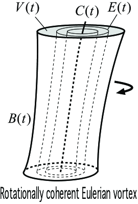
Figure 3: A rotationally coherent Eulerian vortex $V(t)$, with boundary $B(t)$ and vortex center $C(t)$. Also shown within $V(t)$ is a rotational ECS $E(t)$, i.e., a surface along which volume elements exhibit the same intrinsic dynamic rotation rate instantaneously at time $t$. No material coherence is guaranteed for the Eulerian vortex $V(t)$ under passive advection.

Given that

$$\frac{d}{dt}\mathrm{LAVD}_{t_{0}}^{t}(x_{0})=\mathrm{IVD}(x(t;x_{0}),t),$$

rotationally coherent Eulerian vortices are effectively the derivatives of rotationally coherent Lagrangian vortices with respect to the length of the extraction time of the latter. Setting $t=t_{0}$ in (21) and observing that $\mathrm{LAVD}_{t_{0}}^{t_{0}}(x_{0})=0,$ we conclude that the $\mathcal{B}(t_{0})$ initial positions of rotationally coherent Lagrangian vortex boundaries evolve precisely from their Eulerian coherent counterparts $B(t_{0})$ as the Lagrangian extraction time $t_{1}-t_{0}$ increases from zero (see Fig. 4).

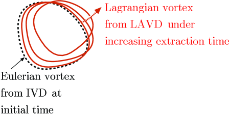
Figure 4: A rotationally coherent Eulerian vortex is the limit of a rotationally coherent Lagrangian vortex under vanishing extraction time (i..e, integration) time.

Physically, these Eulerian vortices are built of tubular surfaces showing instantaneous coherence in the rate of their bulk material rotation. This instantaneous coherence in rotation rates generally does not imply sustained coherence in the finite rotation of material trajectories released from these surfaces. Furthermore, the interior of an evolving vortex $V(t)$ is not a material domain.

By the objectivity of the IVD, Definition 2 nevertheless gives an objective definition of an Eulerian vortex, its center and boundary. To our knowledge, no other objective, three-dimensional Eulerian vortex definition has been proposed in the literature. Specifically, none of the Eulerian criteria reviewed or proposed in Jeung & Hussein (1995), Haller (2005), and Chakraborty, Balachandar & Adrian (2005) are invariant under time-dependent rotations and translations of the observer. Since truly unsteady flows have no distinguished frames of reference (Lugt 1979), non-objective Eulerian vortex criteria do not yield well-defined material vortices for unsteady flows.

A relevant discussion can be found in Jeung & Hussein (1995) about the $\left|\omega\right|$-criterion, by which $\left|\omega\right|$ must exceed a preselect threshold within a vortex. This approach is found intuitive but inadequate in Jeung & Hussein (1995) for several reasons. We agree with this general assessment, because the $\left|\omega\right|$-criterion is threshold-dependent and not objective. In contrast, our rotationally coherent Eulerian vortex definition in Definition 2 is based on a threshold-independent and objective assessment of the level surface topology of $\left|\omega-\bar{\omega}\right|.$

Importantly, for flows with zero mean vorticity in their frame of definition, outermost convex tubular level sets of the vorticity magnitude $\left|\omega\right|$ or of the enstrophy $\left|\omega\right|^{2}$ coincide with rotationally coherent Eulerian vortices. Therefore, when properly interrogated, the vorticity and enstrophy distribution of zero-mean-vorticity flows do reveal objective structures that can be viewed as derivatives of rotationally coherent Lagrangian vortices.

7 Rotationally coherent vortices in planar flows

In a flow defined in the $(x_{1},x_{2})$ plane, the LAVD (18) takes the simple form

$$\mathrm{LAVD}_{t_{0}}^{t}(x_{0})=\intop_{t_{0}}^{t}\left|\omega_{3}(x(s;x_{0}),s)-\bar{\omega}_{3}(s)\right|\,\,ds,$$ (24)

with $\omega_{3}$ referring here to the $x_{3}$ component of the vorticity vector $\omega(x,t)=(0,0,\omega_{3}(x,t))$, and with the mean vorticity $\bar{\omega}_{3}(s)$

By Definition 1, a rotational LCS evolves over the time interval $[t_{0},t_{1}]$ via advection from a closed and convex level curve of the $\mathrm{LAVD}_{t_{0}}^{t_{1}}(x_{0})$ computed in (24). By the same definition, Lagrangian vortex boundaries are outermost members of such rotational LCS families. Similarly, Lagrangian vortex centers are advected positions of isolated maxima of $\mathrm{LAVD}_{t_{0}}^{t_{1}}(x_{0})$.

By Definition 2, a rotational ECS at time $t$ is a closed and convex level curve of

$$\mathrm{IVD}(x,t)=\left|\omega_{3}(x,t)-\bar{\omega}_{3}(t)\right|,$$

around one of its local maxima. Accordingly, rotationally coherent Eulerian vortices are outermost members of such nested curve families with outwards non-increasing instantaneous IVD values.

For two-dimensional flows only, Haller (2016) shows that the relative dynamic rotation angle

$$\phi_{t_{0}}^{t}(x_{0}):=\frac{1}{2}\int_{t_{0}}^{t}\left[\omega_{3}(x(s;x_{0}),s)-\bar{\omega}_{3}(s)\right]\,ds$$

is also an objective and dynamically consistent measure of rotation. It measures the net rotation angle generated by the relative rotation tensor around the $x_{3}$ axis, with sign changes in the rotation accounted for.

While $\psi_{t_{0}}^{t_{1}}(x_{0})$, as the total angle swept by the relative rotation tensor over the time interval $[t_{0},t_{1}]$, is always positive, the sign of the angle $\phi_{t_{0}}^{t_{1}}(x_{0})$ is unrestricted. In vortical regions preserving the pointwise the sign of the Lagrangian vorticity $\omega_{3}(x(s;x_{0}),s)-\bar{\omega}_{3}(s)$, contours of $\phi_{t_{0}}^{t_{1}}(x_{0})$, contours of $\mathrm{LAVD}_{t_{0}}^{t_{1}}(x_{0})$, and contours of the Lagrangian-averaged vorticity (LAV)

$$\mathrm{LAV}_{t_{0}}^{t_{1}}(x_{0}):=\int_{t_{0}}^{t_{1}}\omega_{3}(x(s;x_{0}),s)\,ds$$

all coincide with each other, albeit generally correspond to different values of the underlying scalar fields. In such regions, the sign of $\phi_{t_{0}}^{t_{1}}(x_{0})$ will also carry objective information about the direction of the relative rotation.

Differences in the contours of $\mathrm{LAVD}_{t_{0}}^{t_{1}}(x_{0})$, $\phi_{t_{0}}^{t_{1}}(x_{0})$ and $\mathrm{LAV}_{t_{0}}^{t_{1}}(x_{0})$ will arise in regions where the sign of $\omega_{3}(x(s),s)-\bar{\omega}_{3}(s)$ crosses zero, i.e., near the boundaries of regions with a well-defined sign in their deviation from the mean vorticity of the flow. In such regions, connected level curves of $\mathrm{LAV}_{t_{0}}^{t_{1}}(x_{0})$ can group together initial conditions with substantially different global rotational histories, as long as their final net rotations are equal. The use of $\left.\mathrm{LAVD}\right._{t_{0}}^{t_{1}}(x_{0})$ eliminates such coincidental agreement in the net rotation angles.

8 Geostrophic Lagrangian vortex centers are attractors for inertial particles

Consider a small spherical particle of radius $r_{0}$ and density $\rho_{part}$ in a geostrophic flow of density $\rho$ and viscosity $\nu$. Under the $\beta$-plane approximation, let $f$ denote the Coriolis parameter (twice the local vertical component of the angular velocity of the earth). Applying a slow-manifold reduction to the Maxey–Riley equations (Maxey & Riley 1983) in the limit of small Rossby numbers, Beron–Vera et al. (2015) showed that the inertial particle motion satisfies

$$\dot{x}=v(x,t)+\tau(\delta-1)fJv(x,t)+\mathcal{O}(\tau^{2}),\qquad J=\left(\begin{array}[]{cc}0&-1\\ 1&0\end{array}\right),$$ (25)

where

$$\delta=\frac{\rho}{\rho_{part}},\qquad\tau:=\frac{2r_{0}^{2}}{9\nu\delta}.$$

Provenzale (1999) considered the Maxey–Riley equation in the same physical setting, but without a slow-manifold reduction. His second-order differential equation also included additional terms that either vanish along the $\beta$-plane or appear at higher order in the reduced first-order equation (25) (cf. Beron–Vera et al. 2015 for more detail.)

Remarkably, in the limit of vanishing Rossby numbers, cyclonic attractors for light particles $(\delta>1)$ and anticyclonic attractors for heavy particles $(\delta<1)$ in eq. (25) turn out to be precisely the rotationally coherent vortex centers defined in Definition 1. The same Lagrangian vortex centers act as cyclonic repellers for heavy particles and anticyclonic repellers for light particles. We state these results in more detail as follows:

Theorem 2.

Assume that $x_{0}^{*}\in U(t_{0})$ is the initial position of a rotationally coherent Lagrangian vortex center whose relative rotation keeps constant sign, i.e.,

$$\mathrm{sign}\left[\omega_{3}(x_{0}^{*},t)-\bar{\omega}_{3}(t)\right]=\mu(x_{0}^{*}),\qquad t\in[t_{0},t_{1}],$$ (26)

for an appropriate sign constant $\mu(x_{0}^{*})\in\{-1+1\}$. Then, for $\tau>0$ small enough, the following hold:

(i) In a cyclonic ($\mu(x_{0}^{*})f>0$) rotationally coherent vortex, there exists a finite-time attractor (repeller) for light (heavy) particles that stays $\mathcal{O}(\tau)$ close to the vortex center $\mathcal{C}(t)$.

(ii) In an anticyclonic ($\mu(x_{0}^{*})f<0$) rotationally coherent vortex, there exists a finite-time attractor (repeller) for heavy (light) particles that stays $\mathcal{O}(\tau)$ close to the vortex center $\mathcal{C}(t)$.

Proof: See the Appendix C.

Theorem 2 provides an independent, experimentally verifiable justification for defining vortex centers as in Definition 1 for geostrophic flows. Specifically, positively buoyant drifters or floating debris released well inside a cyclonic oceanic eddy will spiral onto the evolving Lagrangian vortex center identified from Definition 1 (Fig. 5). We will illustrate this effect using simulated inertial particle motion on satellite-based ocean velocities in Section 10.5.

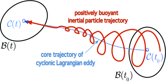
Figure 5: By Theorem 2, cyclonic Lagrangian eddy centers evolving from LAVD maxima act as observed attractors for small, positively buoyant particles, such as drifters and floating debris.

9 Numerical aspects

Computing a rotation angle from the classic polar decomposition requires the computation of the deformation gradient $F_{t_{0}}^{t}$ (cf. (33) in Appendix A). This is either achieved by the numerical differentiation of fluid trajectories with respect to their initial conditions, or by solving the equation of variations $\frac{d}{dt}F_{t_{0}}^{t}=\nabla v(x(t;t_{0},x_{0}),t)F_{t_{0}}^{t}$, whose solutions typically grow exponentially. Either way, computing polar rotation has the same long-time numerical sensitivity that arises in computing the invariants of the Cauchy-Green strain tensor.

In contrast, computing rotationally coherent vortices based on Definition 1 only requires the integration of the normed vorticity deviation along fluid trajectories. This is the simplest to do simultaneously with trajectory integration, solving the extended system of differential equations

$$\frac{dx}{dt} = v(x,t),$$

$$\frac{d}{dt}\mathrm{LAVD}_{t_{0}}^{t} = \left|\nabla\times v(x,t)-\overline{\nabla\times v}(t)\right|,$$ (27)

over a grid of initial conditions over the time interval $[t_{0},t_{1}].$ In our experience, however, features of the $\mathrm{LAVD}_{t_{0}}^{t}(x_{0})$ turn out to be sharper when the trajectory ODE $\dot{x}=v(x,t)$ is solved first, and the vorticity is subsequently integrated along trajectories. This is because adaptive ODE solvers make different decisions about time steps when the trajectory ODE is amended with the ODE for the LAVD field. This is especially so when both ODEs are solved simultaneously over large grids of initial conditions.

The computational domain for solving (27) is just $U(t)\equiv U$ in case of a closed flow with a fixed boundary. In open flows, the focus may be on vortices on a smaller domain. In that case, the domain should still be chosen large enough so that the averaged vorticity $\overline{\nabla\times v}(t)$ is representative of the overall mean rotation of the fluid mass under study. In geophysical flows, this mean rotation is expected to be zero, which is confirmed by our calculations even for domains of the size of a few degrees.

For two-dimensional flows, we first identify local maxima of the LAVD field, then extract nearby closed LAVD level curves. In all our computations, we use the level set function of MATLAB for this purpose, and identify the closedness of a level curve by probing the output from this function. Definition 1 then requires the identification of the outermost convex LAVD level curve around an LAVD maximum as vortex boundary. This convexity requirement is conservative, ensuring that the material vortex starts out unfilamented at the initial time $t_{0}$. At later times, our approach allows for tangential filamentation in the advected LCS due to local strain, but disallows large-scale filamentation arising from differences in the bulk rotation along material filaments. As a consequence, filaments developed by rotational LCSs rotate together with the main body of the underlying material vortex.

In actual computations, one reason to relax strict convexity for closed LAVD level surfaces is that they are numerically represented by discrete polygons. The more vertices such a polygon has, the more likely it is that the polygon is not convex, even if the approximated level curve is. A second reason for relaxing convexity is to remove the conceptual asymmetry of Fig. 2, allowing for small tangential filamentation even in the initial positions of vortex boundaries. A third reason for relaxing strict convexity in multi-scale data sets is the presence of smaller-scale vortices near the perimeter of a larger-scale vortex. This necessitates the use of an appropriately coarse-grained notion for the boundary of the larger vortex.

In two dimensions, addressing the finite-grid, the initial tangential filamentation, and the multi-scale challenges can be achieved by allowing for a small convexity deficiency in the LAVD level curves (Gonzalez & Woods 2008, Batchelor & Whealan 2012). Here, we define the convexity deficiency of a closed curve in the plane as the ratio of the area difference between the curve and its convex hull to the area enclosed by the curve. In Fig. 6, we show cases of closed LAVD level sets with small convexity deficiency. In three dimensions, we require small convexity deficiency for the one-dimensional intersection of LAVD level surfaces with a family $\left\{\mathcal{P}_{i}\right\}$ of planes transverse to the expected vortex center curve $\mathcal{C}(t_{0})$.

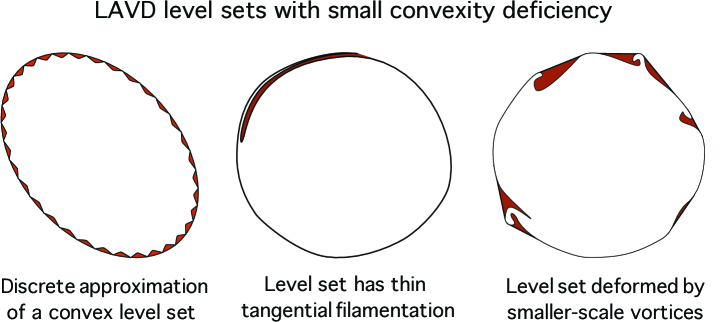
Figure 6: Cases of closed LAVD level sets benefiting from the relaxation of convexity to small convexity deficiency. Shaded area indicates the area difference between the level set and its convex hull. (1) A convex LAVD level set with a non-convex approximating polygon arising from discretization. (2) Closed LAVD level set with minor initial filamentation in the tangential direction. (3) Closed LAVD level set that is only convex after a filtering of smaller-scale vortices.

In our computations, we set the convexity deficiency bound to $10^{-3}$ or lower, which, we find to produce robust results for the first two cases covered in Fig. 6. Applications to multi-scale data sets (last panel of Fig. 6) will likely require a somewhat higher bound. In general, increasing the convexity deficiency bound produces larger eddies that also tend to filament more.

Small-scale local maxima of the LAVD function also arise due to numerical or observational noise in the velocity data. To eliminate the resulting artificial vortex candidates, we choose to ignore closed LAVD contours whose arclength falls below a minimal threshold. In a given application, this threshold should be chosen below the minimal vortex perimeter that is expected to be reliably resolved by the data set.

We summarize the extraction algorithm for rotationally coherent Lagrangian vortices in two- and three-dimensional flows in the tables entitled Algorithm 1 and Algorithm 2 below. The extraction of their rotationally coherent Eulerian counterparts follows the same steps (2)-(4), but applied to the function $\mathrm{IVD}(x,t)$ instead of $\mathrm{LAVD}_{t_{0}}^{t}(x_{0}).$

Algorithm 1 Coherent Lagrangian vortex boundaries and vortex centers for 2-dimensional flows

Input: A 2-dimensional, time resolved velocity field

1. For a two-dimensional grid of initial conditions $x_{0}$, compute the Lagrangian-Averaged Vorticity Deviation $\mathrm{LAVD}_{t_{0}}^{t_{1}}(x_{0})=\int\limits_{t_{0}}^{t_{1}}|\omega_{3}\left(x(s;x_{0}),s\right)-\bar{\omega}_{3}(s)|ds$.

2. Detect initial positions $\mathcal{C}(t_{0})$ of vortex centers as local maxima of $\mathrm{LAVD}_{t_{0}}^{t_{1}}(x_{0})$.

3. Seek initial vortex boundaries $\mathcal{B}(t_{0})$ as outermost, closed contours of $\mathrm{LAVD}_{t_{0}}^{t_{1}}(x_{0})$ satisfying all the following:

   1. $\mathcal{B}(t_{0})$ encircles a vortex center $\mathcal{C}(t_{0})$.

   2. $\mathcal{B}(t_{0})$ has arclength exceeding a threshold $l_{\min}$.

   3. $\mathcal{B}(t_{0})$ has convexity deficiency less than a bound $d_{\max}$.

Output: Initial positions of rotationally coherent Lagrangian vortex boundaries (closed curves) and vortex centers (isolated points) with respect to the time interval $[t_{0},t_{1}].$

Algorithm 2 Coherent Lagrangian vortex boundaries and vortex centers for 3-dimensional flows

Input: A 3-dimensional, time-resolved velocity field

1. For a three-dimensional grid of initial conditions $x_{0}$, compute the Lagrangian-Averaged Vorticity Deviation $\mathrm{LAVD}_{t_{0}}^{t_{1}}(x_{0})=\int\limits_{t_{0}}^{t_{1}}|\omega\left(x(s;x_{0}),s\right)-\bar{\omega}(s)|ds$.

2. Detect initial positions $\mathcal{C}(t_{0})$ of vortex centers as local maximum curves (singular level sets) of $\mathrm{LAVD}_{t_{0}}^{t_{1}}(x_{0})$. This is best done by locating and connecting local maximum points $\hat{\mathcal{C}}_{i}(t_{0})$ of $\mathrm{LAVD}_{t_{0}}^{t_{1}}(x_{0})$ in a family $\left\{\mathcal{P}_{i}\right\}_{i=1}^{N}$ of $N$ parallel planes.

3. Seek initial vortex boundaries $\mathcal{B}(t_{0})$ as outermost tubular level surfaces of $\mathrm{LAVD}_{t_{0}}^{t_{1}}(x_{0})$ whose intersections $\mathcal{\hat{\mathcal{B}}}_{i}(t_{0})=\mathcal{B}(t_{0})\cap\mathcal{P}_{i}$ with the planes $\mathcal{P}_{i}$ satisfy the following for $i=1,\ldots,N$:

   1. $\mathcal{\hat{\mathcal{B}}}_{i}(t_{0})$ encircles a vortex center $\hat{\mathcal{C}}_{i}(t_{0})$.

   2. $\mathcal{\hat{\mathcal{B}}}_{i}(t_{0})$ has arclength exceeding a threshold $l_{\min}$.

   3. $\mathcal{\hat{\mathcal{B}}}_{i}(t_{0})$ has convexity deficiency less than a bound $d_{\max}$.

Output: Initial positions of rotationally coherent Lagrangian vortex boundaries (tubular surfaces) and vortex centers (curves) with respect to the time interval $[t_{0},t_{1}].$

The procedure outlined in Algorithm 2 is mathematically well-defined by the level-surface topology of the LAVD. Step 2 of the algorithm describes one possible numerical extraction scheme for these level surfaces, using their intersections with planes transverse to the anticipated vortex center $\mathcal{C}(t_{0})$. (A MATLAB implementation of this algorithm is available under https://github.com/LCSETH.) Complex flow geometries with multiple vortices and a priori unknown vortex orientations will require more involved numerical approaches to level-set extraction.

To implement Algorithms 1 and 2 in the forthcoming examples, we use a variable-order Adams–Bashforth–Moulton solver (ODE113 in MATLAB) for trajectory advection. The absolute and relative tolerances of the ODE solver are chosen as $10^{-6}$ or higher. In Sections 10.3, 10.4, 10.5 and 11.2, we use cubic and bilinear interpolation schemes for computing pointwise vorticity values for the IVD and LAVD functions, respectively. The lower-order interpolation suffices for the LAVD calculation, because trajectory advection smoothes out the LAVD contours in our experience.

10 Two-dimensional examples

10.1 Planar Euler flows

On any solution of the two-dimensional Euler equation on the $(x_{1},x_{2})$ coordinate plane, the scalar vorticity value $\omega_{3}(x,t)$ is preserved along trajectories. Therefore, the LAVD defined in (18) simplifies to

$$\mathrm{LAVD}_{t_{0}}^{t}(x_{0})=(t-t_{0})\left|\omega_{3}(x_{0},t_{0})-\bar{\omega}_{3}(t_{0})\right|=(t-t_{0})\,\mathrm{IVD}(x_{0},t_{0}),$$

Consequently, at time $t_{0}$, the boundaries and centers of all rotationally coherent Lagrangian vortices coincide with those of rotationally coherent Eulerian vortices. Specifically, ${\cal B}(t_{0})=B(t_{0})$ are outermost, closed and convex level curves of $\left|\omega_{3}(x_{0},t_{0})-\bar{\omega}_{3}(t_{0})\right|$, encircling a local maximum ${\cal C}(t_{0})=C(t_{0})$ of $\left|\omega_{3}(x_{0},t_{0})-\bar{\omega}_{3}(t_{0})\right|$.

If the planar Euler flow is steady, then

$$\frac{d\omega(x(t))}{dt}=\nabla\omega(x(t))\cdot v(x(t))=0.$$

Consequently, as long as the vorticity is not constant on open sets, vorticity contours coincide with streamlines. In that case, both the Lagrangian and the Eulerian vortices are bounded by outermost closed streamlines, with their centers marked by a center-type fixed point, as expected.

Despite these formal LAVD calculations for planar Euler flows, one must remember: the eternal conservation of vorticity in these flows creates a high-degree of degeneracy for the rotation of fluid parcels. Indeed, despite the temporal and spatial complexity of a planar Euler velocity field $v(x,t)$, a fluid element traveling along a fluid trajectory $x(t)$ will keep its initial angular velocity (i..e, half of its vorticity at $t_{0}$ ) for all times $t$. This property locks the initial conditions of initially rotationally coherent fluid parcels to the same LAVD level curve for all times, no matter how much these parcels separate or deform in the meantime. Specifically, even if material filaments break away transversely from a vortical region and undergo high stretching and global filamentation, they will eternally keep the exact same pointwise angular velocity they initially acquired near the vortex (see, e.g., the Eulerian vortex interaction simulation of Dritschel and Waugh 1992 for a striking example).

This rotational degeneracy of the planar Euler equation is lost under the addition of the slightest viscous dissipation, compressibility or three-dimensionality. Under any of these regularizing perturbations, LAVD-based vortex detection can be applied to reveal the Lagrangian signature of vortex interactions in the perturbed flow. We illustrate this in a viscous perturbation of the contour dynamics simulation of Dritschel and Waugh (1992) in Section 10.4.

10.2 Irrotational vortices

Although physically unrealizable, swirling flows with regions of zero vorticity are important theoretical models. The classic irrotational vortex flow is a given by the two-dimensional, circularly symmetric velocity field

$$v(x)=\left(\begin{array}[]{c}\frac{-\alpha x_{2}}{x_{1}^{2}+x_{2}^{2}}\\ \frac{\alpha x_{1}}{x_{1}^{2}+x_{2}^{2}}\end{array}\right).$$ (28)

The vorticity of this flow is identically zero, implying $\mathrm{LAVD}_{t_{0}}^{t}(x_{0})\equiv 0$ and $IVD(x)\equiv 0$ for any choice of $t_{0}$ and $t$. This may seem to be at odds with the fact that all particles move on circular orbits, and hence line elements tangent to the trajectories exhibit one full rotation over the period of the circular orbit.

However, the tangents are special line elements and are not representative of the overall bulk rotation of fluid elements. Material fibers transverse to the trajectory tangents all rotate at different speeds. The average rate of rotation for all line elements emanating from a given point is zero, as was already pointed out by Helmholtz (1858) in a related debate with Bertrand (1873) (cf. Truesdell & Rajagopal 2009, Haller 2016). Therefore, an infinitesimal fluid volume has no experimentally measurable bulk rigid-body rotation component in its deformation, as indeed demonstrated by Shapiro (1961).

The irrotational vortex flow (28) is composed of a single, degenerate LAVD and IVD level set $\mathrm{LAVD}_{t_{0}}^{t}(x_{0})=\mathrm{IVD}(x)\equiv 0$, as opposed to a nested family of codimension-one tubular level sets with outward decreasing LAVD and IVD values. Therefore, the flow (28) does not satisfy our Definitions 1 and 2, and hence does not qualify as a rotationally coherent Lagrangian or Eulerian vortex. A similar conclusion holds on the irrotational domains of the Rankine and the Lamb–Oseen vortices (Majda & Bertozzi 2002), or more generally, in a recirculation region of any potential flow. We note that irrotational vortices are also either explicitly excluded by most systematic vortex criteria or fail the test for being a vortex according to these criteria.

10.3 Direct numerical simulation of two-dimensional turbulence

We solve numerically the forced Navier–Stokes equation

$$\partial_{t}v+v\cdot\nabla v=-\nabla p+\nu\Delta v+f,\qquad\nabla\cdot v=0,$$ (29)

for a two-dimensional velocity field $v(x,t)$ with $x=(x_{1},x_{2})\in U=[0,2\pi]\times[0,2\pi]$. We use a pseudo-spectral code with viscosity $\nu=10^{-5}$. We evolve a random-in-phase velocity field in the absence of forcing ($f=0$) until the flow is fully developed, then turn on a random-in-phase forcing (cf. Farazmand et al. 2013). We identify this latter time instance with the initial time $t_{0}=0$, and run the simulation till the final time $t_{1}=50.$

To construct the LAVD field, we advect trajectories from an initial grid of $1024\times 1024$ points over the time interval $[0,50]$. We integrated the vorticity deviation norm separately (as opposed to solving the combined ODE (27)), using 1200 vorticity values along each trajectory, equally spaced in time. Figure 7 shows the results superimposed on the contours of $\mathrm{LAVD}_{0}^{50}(x_{0})$. In this computation, we have set the minimum arc-length, $l_{\mathrm{min}}=0.3$ and convexity deficiency bound $d_{\mathrm{max}}=10^{-4}$.

Figure 7 shows the Lagrangian vortex boundaries extracted from Definition 1 using Algorithm 1 at the initial time $t_{0}=0$. In Figure 7, we confirm the Lagrangian rotational coherence of these vortex boundaries by advecting them to the final time $t_{1}=50$. As expected, the vortex boundaries do not give in the general trend of exponential stretching and folding observed for generic material lines. Instead, they display only local (tangential) filamentation. The complete advection sequence over the time interval $[0,50]$ is illustrated in the online supplemental movie M1.

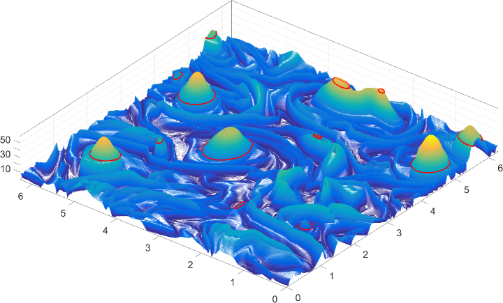
(a)

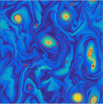
(b)

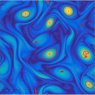
(c)

Figure 7: (a) Three-dimensional contour plot of $\mathrm{LAVD}_{0}^{50}(x_{0})$. Lagrangian vortex boundaries (outermost rotational LCSs) extracted from Algorithm 1 are shown in red. (b) Vortex boundaries shown in the flow domain at initial time $t=0$. Shown in the background is the contour plot of $\mathrm{LAVD}_{0}^{50}(x_{0})$ for reference.(c) Advected Lagrangian vortex boundaries at the final time $t_{1}=50$. (See the on-line supplemental movie M1 for the complete advection sequence of the vortex boundaries).

In Fig. 8a, we show the time $t_{0}$ positions of rotationally coherent Eulerian vortices in green, along with their Lagrangian counterparts in red. Passively advected positions of the Eulerian vortices are shown in Fig. 8b, displaying substantial material fingering into their surroundings. While this lack of full material coherence over time is expected for the Eulerian vortices, some of them are impressively close to their Lagrangian counterparts at the initial time $t_{0}$, even though they are extracted just from an instantaneous analysis. At the same times, other Eulerian vortices without nearby Lagrangian counterparts disintegrate completely under advection, as seen in Fig. 8b.

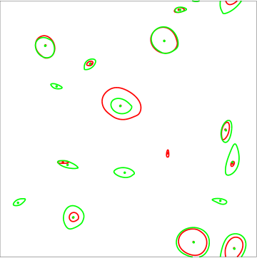
(a)

(b)

(c)

Figure 8: (a) Lagrangian (red) and Eulerian (green) rotationally coherent vortices at time $t_{0}$ in the two-dimensional turbulence example. (b) Rotationally coherent Eulerian vortex boundaries and centers at time $t_{0}$, with the $\mathrm{IVD}(x,t_{0})$ field shown in the background. (c) The same objects advected passively to the final time $t_{1}=50$, with $\mathrm{IVD}(x,t_{1})$ shown in the background.

10.4 Interaction of two unequal vortices

Motivated by the inviscid contour-dynamics simulation of Dritschel & Waugh (1992), we seek to identify Lagrangian vortex cores in the interaction of two vortices of unequal strength (cf. our discussion in Section 10.1). We solve the Navier–Stokes equation (29) in two dimensions with viscosity $\nu=2\times 10^{-6}$. As initial velocity field, we let

$$v(x,0)=v_{1}(x)+v_{2}(x),\qquad v_{i}(x)= \Gamma_{i}\frac{1-\exp(-r_{i}^{2}/\delta_{i}^{2})}{2\pi r_{i}^{2}}\,R_{\pi/2}\,(x-x_{i}),\quad i=1,2,$$

where $r_{i}^{2}=|x-x_{i}|^{2}$ , and the matrix $R_{\pi/2}$ refers counter-clockwise rotation by $\pi/2$. Each $v_{i}$ defines a vortex centered at a point $x_{i}$ with a Gaussian profile. The parameters $\Gamma_{i}$ and $\delta_{i}$ control the strength and width of each vortex, respectively. In our simulation. we chose

$$\Gamma_{1}=0.01,\quad\delta_{1}=0.05,\quad x_{1}=(\pi,\pi+0.2),$$

$$\Gamma_{2}=0.12,\quad\delta_{2}=0.20,\quad x_{2}=(\pi,\pi-0.2).$$

The vortex described initially by $v_{1}$ is, therefore, weaker and smaller, and hence is expected to deform significantly under the strain field created by the second vortex initially described by $v_{2}$. The computational domain is $x\in[0,2\pi]\times[0,2\pi]$, discretized into $512\times 512$ grid points. During the simulation, the vortices stay far enough from the boundary so that the boundary effects on their evolution are negligible. A relevant Reynolds number can be computed as $Re=\Gamma_{2}/\nu=6\times 10^{4}$ (cf. Kevlahan & Farge 1997). For this Reynolds number, the flow still remains fairly close to its inviscid limit, with the standard deviation of the vorticity from its initial value staying below $0.5\%$ along fluid trajectories.

We have run the computation from the non-dimensional time $t_{0}=0$ up to $t=30.$ Over this time scale, we could preserve the smoothness of the velocity field without additional numerical effort. We applied Algorithm 1 with the tight convexity deficiency $d_{max}=10^{-3}$ and the arclength filter $l_{min}=0.1$. We show the rotationally coherent vortex boundaries obtained in this fashion in Fig. 9, along with two other closed material lines initiated around the vortex cores. The latter two circles approximate closely the Eulerian vorticity boundaries inferred from the instantaneous vorticity at time $t_{0}=0$. They, therefore, mimic the the role of the initially circular vorticity jump contours advected in the inviscid simulation of Dritschel & Waugh (1992).

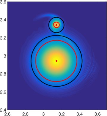
(a)

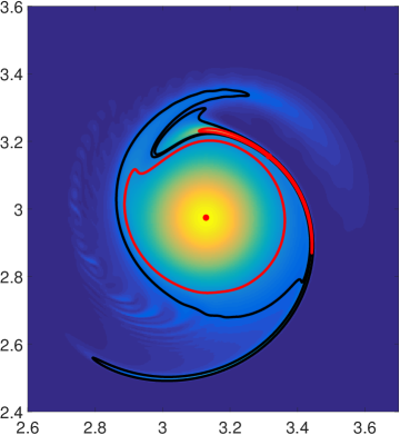
(b)

Figure 9: (a) Rotationally coherent Lagrangian vortex boundaries (red) at time $t_{0}=0$ in the vortex interaction example. Also shown are two circles (black) approximating the Eulerian vortex boundaries inferred at time $t_{0}$ from the vorticity distribution. The $LAVD_{0}^{30}(x_{0})$ is shown in the background for reference. (b) advected position of the Lagrangian vortex boundaries and the two closed material curves at time $t=30.$ The advected LAVD field $LAVD_{0}^{30}(x(30;0,x_{0}))$ is shown in the background. (See the on-line supplemental movie M2 for the complete advection sequence of the vortex boundaries).

As seen in Fig. 9, the stronger Eulerian vortex creates a sizable rotationally coherent Lagrangian vortex in the center. This vortex shows only tangential filamentation, as confirmed by its advected position at $t=30$. The weaker Eulerian vortex has a substantially smaller coherent Lagrangian footprint that orbits around the larger vortex.

This weaker satellite vortex gradually reaches a maximal elongated perimeter at about $t=24$, then preserves its arclength in an approximate rigid-body rotation for the remaining $20\%$ of the simulation time. No transverse filamentation occurs in this case either: the satellite vortex remains rotationally coherent in the sense of our Definition 1.

Therefore, as Figure 9 illustrates, two unequal viscous vortices may interact strongly and still preserve their rotationally coherent material cores during a finite time interval of their interaction. Such coherent cores remain hidden in contour dynamics studies focused on the advection of Eulerian vortex boundaries inferred from large initial vorticity gradients. Indeed, the two black material curves of Figure 9, mimicking the role of vortex-bounding inviscid vorticity contours, develop substantial transverse filamentation during the same time interval.

10.5 Two-dimensional Agulhas eddies in satellite altimetry

Here we illustrate the detection of rotationally coherent eddy boundaries in velocity data derived from satellite-observed sea-surface heights under the geostrophic approximation. In this approximation, the satellite-measured sea-surface height $\eta(\varphi,\theta,t)$ serves as a non-canonical Hamiltonian for surface velocities in $(\varphi,\theta)$ longitude-latitude $(\varphi,\theta)$ coordinate system.

The evolution of fluid particles satisfies

$$\dot{\varphi}(\varphi,\theta,t) = -\frac{g}{R^{2}f(\theta)\cos\theta}\ \partial_{\theta}\eta(\varphi,\theta,t),$$ (30)

$$\dot{\theta}(\varphi,\theta,t) = \frac{g}{R^{2}f(\theta)\cos\theta}\ \partial_{\varphi}\eta(\varphi,\theta,t),$$ (31)

where $g$ is the constant of gravity, $R$ is the mean radius of the Earth, and $f(\theta)\equiv 2\Omega\sin\theta$ is the Coriolis parameter, with $\Omega$ denoting the Earth’s mean angular velocity. The publicly available AVISO sea-surface height data base for $\eta(\varphi,\theta,t)$ is given at a spatial resolution of $1/4^{\circ}$ and a temporal resolution of $7$ days.

We select the computational domain in the longitudinal range $[-4^{\circ},9^{\circ}]$ and the latitudinal range $[-35^{\circ},-28{}^{\circ}]$, which falls inside the region of the Agulhas leakage in the Southern Ocean. A Lagrangian analysis of coherent mesoscale eddies is particularly important in this context, as the amount of warm and salty water carried from the Indian Ocean to Atlantic Ocean has relevance for global circulation and climate (Beal et al. 2011).

Recent two-dimensional Lagrangian studies of the Agulhas leakage used geodesic LCS theory to locate perfectly non-filamenting (black-hole type) material eddies (Haller & Beron–Vera 2013, Beron–Vera et al. 2013). Here we use a relaxed notion of coherence, which allows for tangential filamentation, but not for global break-away of material from the eddy. The computational cost in the present method is substantially lower: the calculation of the deformation gradient and the search for limit cycles bounding the black-hole eddies are absent.

We consider the AVISO data set ranging from the initial time $t_{0}=\mathrm{November}\,11,\,2006$ to the final time $t_{1}=t_{0}+90\,\mathrm{days}$. We select an initial grid of particles with stepsize $\Delta x_{0}=1/50^{\circ}$. As an additional filter for eliminating LAVD and IVD maxima due to resolution coarseness, we ignore from the start LAVD and IVD maxima that are closer than the submesoscale distance $0.2^{\circ}$ (about 20 km). As a complexity deficiency bound, we select $d_{\max}=10^{-3}$. As an arclength threshold, we fix $l_{\min}=2\pi r$, with $r=20$ km selected again as a lower bound on mesoscale structures reliably resolved by altimetry.

Beyond executing Algorithm 1 to extract rotationally coherent in this setting, we also use this example to illustrate the predictions obtained from Theorem 2 for the attractor role of rotationally coherent Lagrangian vortex centers. Figure 10a shows the rotationally coherent eddies, while Figure 10b confirms that their boundaries only develop tangential filamentation under Lagrangian advection, as expected. This second plot also confirms that LAVD-based vortex centers are precisely the observed attractors for light particles released in cyclonic eddies, and for heavy particles released in anticyclonic eddies.

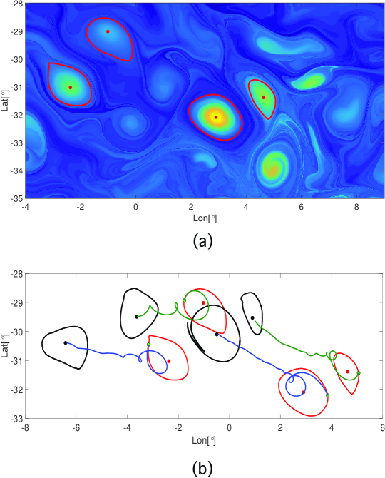
Figure 10: (a) Rotationally coherent Lagrangian vortices at time $t_{0}=\mathrm{November}\,11,\,2006$, identified from Algorithm 1 using the contours of $\mathrm{LAVD}_{t_{0}}^{t_{0}+T}(x_{0})$ with $T=90\,\mathrm{days}$. Shown in the background is the contour plot of $\mathrm{LAVD}_{t_{0}}^{t_{0}+T}(x_{0})$ for reference. (b) Initial (red) and final (black) positions of the Lagrangian vortex boundaries at time $t_{0}+T$, along with representative inertial particle trajectories. Heavy particles (blue) converge to the centers of anti-cyclonic (clockwise) eddies. Light particles (green) converge to the centers of cyclonic (clockwise) eddies. Here $\delta_{heavy}=0.99$, $\delta_{light}=1.01$, $r_{0}=1$ m. (See the on-line supplemental movie M3 for the complete advection sequence of the vortex boundaries and the inertial particles).

We show a comparison of the initial positions of rotationally coherent Lagrangian and Eulerian vortices in Fig. 11a. Three of the Eulerian eddies (green) are close to Lagrangian eddies (red), and will accordingly show some coherence under advection by the end of the observational period in Fig. 11c. The remaining Eulerian eddies show major filamentation and disintegrate under advection. We note the large number of false positives for coherent eddies based on the instantaneous Eulerian prediction at the initial time, even though this prediction is frame-invariant.

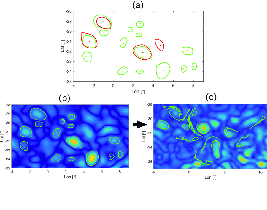
Figure 11: (a) Lagrangian (red) and Eulerian (green) rotationally coherent vortices at time $t_{0}$ in the satellite altimetry example. (b) Rotationally coherent Eulerian vortex boundaries and centers at time $t_{0}$, with the $\mathrm{IVD}(x,t_{0})$ field shown in the background. (c) The same objects advected passively to the final time $t_{1}=t_{0}+T$, with $\mathrm{IVD}(x,t_{1})$ shown in the background.

In Appendix D, we also use this example to illustrate differences between LAVD-based vortex detection and two other objective Lagrangian tools for two-dimensional flows: the geodesic LCS approach of Haller & Beron–Vera (2013) and the ellipticity-time diagnostic of Haller (2001).

We find that the geodesic LCS approach generally identifies similar material vortex regions as LAVD. By construction, however, geodesic vortex boundaries enclose perfectly non-filamenting vortex cores, and hence miss the rotationally coherent (but tangentially filamenting) outer annuli of Lagrangian vortices. The identification of the perfectly coherent, black-hole-type core by the geodesic LCS approach also comes with a higher computational cost and does not extend to three dimensions (cf. Appendix D for details).

We also find that the ellipticity-time diagnostic highlights the general vicinity of the coherent material vortex regions, but offers no well-defined procedure for defining vortex boundaries. Focused on individual trajectory stability rather than global coherence, the ellipticity time has equally high values in some regions that do not remain coherent as a whole. Conversely, the ellipticity time indicates predominantly hyperbolic (i.e., non-vortical) behavior in the outer, tangentially filamenting parts of rotationally coherent vortices.

In summary, despite their higher computational costs, neither globally uniform-stretching material lines nor elliptic fluid trajectories are able to provide the large, coherent material vortex boundaries obtained from the LAVD.

11 Three-dimensional examples

11.1 Strong Beltrami flows

Strong Beltrami flows are steady flows whose vorticity field is a constant scalar multiple of the velocity field (Majda & Bertozzi 2002), i.e.

$$\omega(x)=\lambda v(x).$$

In this case, formula (18) gives

$$\left.\mathrm{LAVD}\right._{t_{0}}^{t}(x_{0})=\left|\lambda\right|\intop_{t_{0}}^{t}\left|v(x(s))-\bar{v}\right|ds,\qquad\bar{v}:=\frac{1}{\mathrm{vol}\,(U)}\int_{U}v(x)\,dV.$$ (32)

Thus, for any strong Beltrami flow with $\lambda\neq 0$, a rotationally coherent Lagrangian vortex boundary is a locally outermost, closed and convex level surface of $\intop_{t_{0}}^{t}\left|v(x(s))-\bar{v}\right|ds,$ the trajectory-averaged deviation of the velocity field from its spatial mean. For general 3D steady flows, level sets of asymptotically Lagrangian-averaged observables have been noted to approximate ergodic components (Budišić & Mezić 2012). The new result here is that tubular levels sets of the finite-time average of the normed velocity deviation in strong Beltrami flows specifically define rotationally coherent Lagrangian structures (surfaces of constant net bulk rotation) in an objective fashion.

By formula (32), rotationally coherent Eulerian vortices in strong Beltrami flows are composed of convex tubular level surfaces of the normed velocity deviation $\mathrm{IVD}(x)=$$\left|v(x)-\bar{v}\right|$.

As an example, we consider the ABC flow whose velocity field is given by

$$v(x)=\left(\begin{array}[]{c}A\sin x_{3}+C\cos x_{2}\\ B\sin x_{1}+A\cos x_{3}\\ C\sin x_{2}+B\cos x_{1}\end{array}\right)$$

over the triply periodic domain $U=[0,2\pi]^{3}$. A direct calculation gives $\bar{v}(x)\equiv 0$ and $\lambda=1$. We select the parameter configuration $A=1,$ $B=\sqrt{2/3}$, and $C=\sqrt{1/3}$. For our Lagrangian advection, we select an initial grid of $200^{3}$ evenly distributed particles, which we advect over the interval $[t_{0},t_{1}]=[0,50]$.

Figure 12a shows three representative Lagrangian vortex boundaries obtained as outermost, convex tubular level surfaces of $\left.\mathrm{LAVD}\right._{0}^{50}(x_{0})$. By the simplicity of this steady flow, relaxing convexity was not necessary (the convexity deficiency is zero). Also shown in Figure 12 are trajectory-segments launched along the Lagrangian vortex boundaries, illustrating their Lagrangian invariance. Figure 12b shows the single IVD-based Eulerian vortex obtained for the ABC flow. While this Eulerian structure is near one of the Lagrangian vortices, the shape of the IVD-based vortex is not representative of the true Lagrangian vortex in this example. Furthermore, no IVD-based Eulerian vortices arise near the remaining Lagrangian vortices. This might seem puzzling first, but one must remember the spatial anisotropy of the ABC flow for unequal $A,B$ and $C$ parameter values.

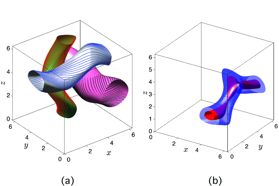
Figure 12: (a) Three representative rotationally coherent Lagrangian vortex boundaries in the ABC flow, obtained as outermost, convex tubular level sets of $\left.\mathrm{LAVD}\right._{0}^{50}(x_{0})$. Black curves indicate trajectories launched on these boundaries. (b) Two representative $\mathrm{IVD}(x_{0})$ level surfaces (with blue denoting the rotationally coherent Eulerian vortex boundary) in the single Eulerian coherent vortex obtained from the IVD field for the ABC flow for the parameter values considered here.

11.2 Three-dimensional Agulhas eddies in a data-assimilating circulation model

Here we apply LAVD-based vortex extraction to a three-dimensional unsteady velocity field set obtained from the Southern Ocean State Estimation (SOSE) model (Mazloff, Heimbach & Wunsch 2012). The domain of the data set is again in the area of the Agulhas leakage in the Southern Ocean, representing a three-dimensional extension of the Agulhas eddy extraction study of Section 10.5.

Our Lagrangian study covers a period of $T=120\,\mathrm{days}$, ranging from $t_{0}=$ 15 May 2006 to $t=$ 12 September 2006. The selected computational domain in the South Atlantic ocean is bounded by longitudes $[11^{\circ}\text{E},16^{\circ}\text{E}]$, latitudes $[37^{\circ}\text{S},33^{\circ}\text{S}]$, and depths $[7,2000]$ meters. We compute the LAVD and IVD fields over a uniform grid of $350\times 350\times 350$ points, and identify a rotationally coherent Lagrangian and Eulerian vortices using Algorithm 2. As in our two-dimensional turbulence example, we integrate the vorticity deviation norm separately (as opposed to solving the combined ODE (27)), using 1000 vorticity values along each trajectory, equally spaced in time. For the plane family $\mathcal{P}_{i}$ featured in Algorithm 2, we consider horizontal planes along nodes of the initial grid, starting from 28 meters below the sea surface level to eliminate noise due to boundary effects at the surface. In these planes we use the arclength threshold $l_{\min}=0.1$ and the maximal convexity deficiency $d_{\max}=10^{-4}.$ The spatial mean vorticity $\bar{\omega}(t)$, as the practically observed mean vorticity for a large enough fluid mass in the ocean, is taken to be zero.

Figure 13a shows the initial position of a rotationally coherent Lagrangian eddy boundary (yellow) and its center (red), extracted as a level sets of $\mathrm{LAVD}_{t_{0}}^{t_{1}}(x_{0})$ by Algorithm 2. Also shown is a nearby LAVD level surface outside the eddy boundary, illustrating the complexity of the near-surface mixing region enclosing the eddy. Figure 13b gives a full view of the Lagrangian eddy, whereas Figure 13c shows the materially advected position of the eddy at the final time, $120$ days later. As expected, there is mild tangential filamentation in the material eddy boundary, but strictly no break-away from the rotating water mass. Given the complexity of material mixing in the surrounding waters, this high degree of material coherence illustrates well the accuracy of LAVD-based vortex extraction.

(a)

(b)

(c)

Figure 13: (a) Representative level surfaces of $\mathrm{LAVD}_{t_{0}}^{t_{0}+T}(x_{0})$ with $t_{0}=\mathrm{May}\,15,\,2006$ and $T=120$ days.  The yellow surface is extracted using Algorithm 2, marking the vortex boundary for a mesoscale, rotationally coherent Lagrangian eddy, extending from $28$ meters down to $646$ meters in depth. The green surface is a nearby level surface of $\mathrm{LAVD}_{t_{0}}^{t_{0}+T}(x_{0})$ outside the Lagrangian vortex region. The red curve marks the coherent vortex center, as defined in Definition 1. (b) Full view of the Lagrangian eddy boundary and its center at the initial time $t_{0}$ (c) The advected eddy boundary and vortex center $120$ days later, extending from 49 meters down to 726 meters below the surface (See the on-line supplemental movie M4 for the complete advection sequence of the eddy boundary).

The corresponding rotationally coherent Eulerian eddy extracted at the same initial location, then materially advected for 120 days, is shown in Fig. 14. In the Eulerian computation, noise in the level surface computation is more moderate than in the Lagrangian case. As a result, the plane family $\mathcal{P}_{i}$ featured in Algorithm 2 can be selected to start from as high as 7 meters below the surface.

This Eulerian eddy has about the same diameter near the sea surface as its Lagrangian counterpart, but maintains this diameter and reaches to substantially larger depths. Its vertical size is further increased under advection, with the bottom forming a sharp tip. Overall, the advected surface shows high ribbing and filamentation. Large-scale material break-away is absent in this example, but this cannot be guaranteed a priori for an Eulerian eddy (see our two-dimensional computations in Section 10.5). A comparison of Figures 13 and 14 suggests that the Lagrangian eddy forms a smooth, coherent center region that transports water without observable filamentation inside the vortical Eulerian feature.

(a)

(b)

Figure 14: (a) The rotationally coherent Eulerian counterpart of the Lagrangian eddy shown in Figure 13a, ranging from 7 $m$ down to 1,007 $m$ below the see surface. (b) The materially advected position of the Eulerian eddy 120 days later, ranging from 15 $m$ to 1,163 $m$ below the sea surface (See the on-line supplemental movie M5 for the complete advection sequence of the eddy boundary).

With a larger number of dedicated control points, the computation of LAVD level surfaces can be extended closer to the ocean surface. Figure 15 shows a higher-resolution computation of the initial and advected positions of the top slices of IVD-based and LAVD-based rotationally coherent vortex boundary surfaces. In this computation, the initial top slice of the LAVD-based vortex boundary is located only $15$ $m$ below the ocean surface, as opposed to the $28$ $m$ distance used in Fig. 13c. Even this Lagrangian boundary slice remains more coherent than the Eulerian one, but the Eulerian slice still performs well under material advection for this eddy and for this advection time.

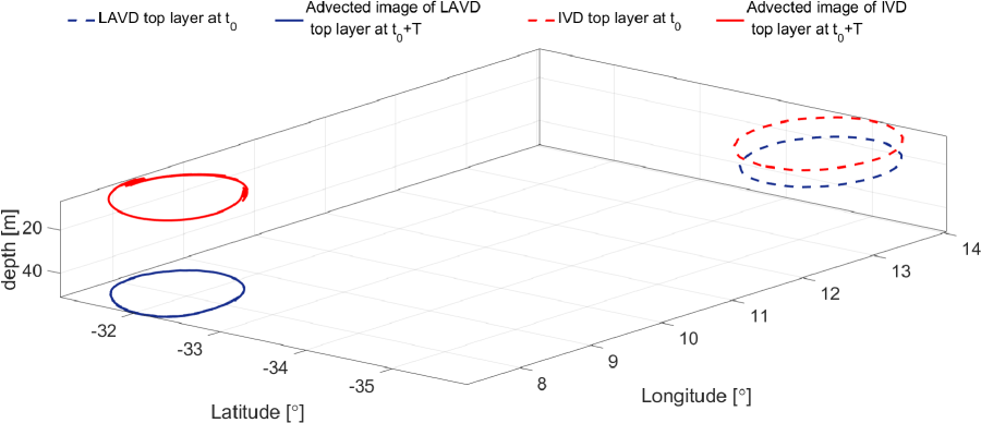
Figure 15: Initial top slices (dashed line, at time $t_{0}=\mathrm{May}\,15,\,2006$) and their advected positions (solid line, $T=120\,days$ later) of the LAVD- and IVD-based rotationally coherent vortex boundaries.

12 Conclusions

We have given an objective (fully observer-independent) definition of a Lagrangian vortex as a set of material tubes in which fluid elements complete the same intrinsic dynamic rotation. This material rotation angle is obtained from the exact, dynamically consistent decomposition (20) of the deformation gradient. Remarkably, the intrinsic material rotation angle is expressible as the trajectory integral of the normed deviation of the vorticity from its spatial mean (LAVD). The intrinsic material rotation is, therefore, directly observable as the rotation of vorticity-meters in fluid experiments (Shapiro 1961), once the mean rotation reported by these devices is subtracted from the measurements.

Locating a rotationally coherent material vortex does not require advection of high-density material grids, a generally taxing numerical procedure in Lagrangian coherence calculations. By construction, LAVD-based material vortices may show material filamentation, but even filamented material elements will rotate together with the vortex without global breakaway. The vortex interior, therefore, shows no advective mixing with its environment, as we have illustrated on several several examples in two- and three-dimensional unsteady flows.

Our approach also enables the extraction of vortex centers as singular level sets (local maxima) of the LAVD. We have proved that in two-dimensional geostrophic flows, these vortex centers coincide precisely with attractors of light particles in cyclonic eddies and for heavy particles in anticyclonic eddies. Indeed, we have found that numerically simulated light and heavy inertial particles show quick convergence to the appropriate moving vortex cores in a satellite-inferred, geostrophic ocean velocity field. On the same example, we have illustrated the advantages of LAVD-based coherent vortex detection compared to other objective Lagrangian vortex detection tools.

The deviation of potential vorticity from its spatial mean is tempting to consider for a similar analysis, but such an approach would remain heuristic, driven purely by analogy. This is because potential vorticity is not objective and cannot be rigorously connected to intrinsic material rotation generated by the deformation gradient.

Motivated by our results on LAVD, one might proceed by analogy and probe plots of Lagrangian averages of arbitrary scalar fields for vortical features. As long as these scalar fields are non-degenerate and favorably initialized, material vortices should indeed have a footprint in the resulting plots due to the coherence of trajectories in the vortex interiors. For instance, the trajectory-averaged Okubo–Weiss parameter (Dresselhaus & Tabor 1989, P rez–Mu uzuri & Huhn 2013) and trajectory-averaged helicity (P rez–Mu uzuri & Huhn 2013) may also have lows and highs, respectively, near material vortices. Such extrema are, however, heuristic diagnostics, each signaling a different domain for a vortex, and each showing extrema in other flow regions as well. Their features are a consequence, rather than a well understood root cause, of material coherence (cf. Beron–Vera 2015).

In contrast, we arrive here at LAVD-based vortices by solving an objectively posed coherence problem for material surfaces of equal bulk rotation. The LAVD then arises from an exact, dynamically consistent decomposition of the deformation gradient into purely rotational and purely straining deformation gradients. The vortex boundaries and centers so obtained are sharply defined, do not develop global material filamentation, and remain invariant with respect to all possible Euclidean observer changes.

We have also formulated an objective Eulerian definition of a rotationally coherent vortex: a domain filled with tubular surfaces of constant intrinsic material rotation rate. These surfaces coincide with outward-decreasing tubular level sets of the instantaneous vorticity deviation (IVD). In some cases, we have found rotationally coherent Eulerian vortices and their centers to be surprisingly close to their Lagrangian counterparts. While such closeness does not hold in general, IVD-based vortices do provide a systematic and frame-invariant way to track coherent velocity features that are infinitesimally consistent in time with coherent material vortices. This makes these Eulerian vortices and vortex centers appropriate tools for a fully frame-invariant, automated vortex census in turbulent flow data.

Acknowledgements

We acknowledge helpful discussions with Matt Mazloff, and exploratory work by Dan Blazevski on the SOSE data set. We are grateful to one of the anonymous reviewers of this paper for suggesting the example considered in Section 10.4 and the comparison carried out in Appendix D. The altimeter products used in this work are produced by SSALTO/DUACS and distributed by AVISO, with support from CNES (http://www.aviso.oceanobs.com/duacs).

13 Appendix A: Material rotation from the classical Polar Decomposition

Finite strain theory (Truesdell & Noll 1965) infers a unique bulk material rotation for material volume elements between times $t_{0}$ and $t_{1}$ from the polar decomposition

$$F_{t_{0}}^{t_{1}}=R_{t_{0}}^{t_{1}}U_{t_{0}}^{t_{1}},\qquad R_{t_{0}}^{t_{1}}=F_{t_{0}}^{t_{1}}\left[C_{t_{0}}^{t_{1}}\right]^{-1/2},\qquad U_{t_{0}}^{t_{1}}=\left[C_{t_{0}}^{t_{1}}\right]^{1/2},$$ (33)

of the deformation gradient. Here the rotation tensor $R_{t_{0}}^{t_{1}}$ is proper orthogonal, interpreted as the solid-body rotation component of the deformation. The right stretch tensor, $U_{t_{0}}^{t_{1}}$, is symmetric and positive definite, obtained as the principal square root of the Cauchy–Green strain tensor $C_{t_{0}}^{t_{1}}$. The right stretch tensor is interpreted as the stretching preceding the solid-body rotation represented by $R_{t_{0}}^{t_{1}}$. The tensors $R_{t_{0}}^{t_{1}}$ and $U_{t_{0}}^{t_{1}}$ are not objective, but the eigenvalues of $U_{t_{0}}^{t_{1}}$ are preserved under time-dependent rotations and translations (Truesdell & Noll 1965).

In a given frame of reference, $R_{t_{0}}^{t_{1}}(x_{0})$ represents the unique rotation that gives the closest fit to the linear operator $F_{t_{0}}^{t_{1}}(x_{0})$ in the Frobenius matrix norm (Gollub & Van Loan 1983). In two and three dimensions, the action of $R_{t_{0}}^{t_{1}}(x_{0})$ can be described by a single polar rotation angle (PRA). Well-defined up to multiples of $2\pi$, PRA is the signed angle of rotation along the axis of rotation associated with the tensor $R_{t_{0}}^{t_{1}}(x_{0})$

In recent work, we used tubular and singular level surfaces of the PRA to visualize elliptic Lagrangian regions and their centers, respectively (Farazmand & Haller 2016). To our knowledge, this represents the first systematic approach to identifying Lagrangian coherence based on a synchrony in the net material rotation of infinitesimal volume elements. The level sets of PRA are objective in two dimensions, and have shown themselves to be accurate indicators of elliptic regions in unsteady flows with general time dependence.

Nevertheless, several challenges remain that the classic polar decomposition, and hence also the PRA, are unable to address:

1. PRA level sets are not frame-invariant in three dimensions. Therefore, PRA in three dimensions cannot be used to define elliptic LCSs, which are material (and hence fundamentally frame-invariant) surfaces.

2. The computation of the PRA is based on the invariants of the Cauchy–Green strain tensor. This requires the accurate differentiation of the flow map $\mathcal{F}_{t_{0}}^{t_{1}}(x_{0})$ with respect to initial conditions. This is numerically costly for extended times in large flow domains.

3. No straightforward relationship exists between finite material rotation represented by the PRA and physical quantities (most notably, vorticity) used in Eulerian vortex identification. Indeed, only an involved link exists between $R_{t_{0}}^{t_{1}}$ and the spin tensor $W$ through the formula

   $$\dot{R}_{t_{0}}^{t}=\left(W-\frac{1}{2}R_{t_{0}}^{t}\left[\dot{U}_{t_{0}}^{t}\left(U_{t_{0}}^{t}\right)^{-1}-\left(U_{t_{0}}^{t}\right)^{-1}\dot{U}_{t_{0}}^{t}\right]\left(R_{t_{0}}^{t}\right)^{T}\right)R_{t_{0}}^{t},$$ (34)

   where dot refers to differentiation with respect to $t$ (Truesdell & Rajagopal 2009).

4. Between two fixed times $t_{0}$ and $t_{1}$, the polar rotation tensor $R_{t_{0}}^{t_{1}}$ represents the closest solid-body rotation to $F_{t_{0}}^{t_{1}}$ in the Frobenius norm. For intermediate times $t\in[t_{0},t_{1}],$the rotation family $R_{t_{0}}^{t}$ provides no self-consistent solid-body rotation component for the evolving deformation gradients $F_{t_{0}}^{t}$ . Indeed, one generally has

   $$R_{t_{0}}^{t}\neq R_{s}^{t}R_{t_{0}}^{s},\qquad s,t\in[t_{0},t_{1}],$$ (35)

   which means that the rotation family $R_{t_{0}}^{t}$ does not satisfy the basic superposition principle of subsequent rigid-body rotations. Consequently, experimentally observed finite material rotation in fluids (visualized by small rigid-body tracers (Shapiro 1961) will differ from the PRA even in the simplest flows (see Haller 2016 for further discussion).

Haller (2016) also discusses the rotational component yielded by $R_{t_{0}}^{t}$ for two simple fluid-mechanical examples: irrotational vortices and parallel shear flows. In these examples, observed material rotation signaled by small inertial tracers (vorticity-meters) differs fundamentally from the rotation captured by $R_{t_{0}}^{t}$.

14 Appendix B: Rotationally coherent vortices in flow over a moving surface

Here we show how the LAVD and IVD can be computed over moving surfaces, such as the rotating Earth, without having to compute vorticity in the curvilinear coordinates. Consider first a three-dimensional spatial domain $U(t)\subset\mathbb{R}^{3}$ that possibly also translates and rotates in time. We assume that $U(t)$ admits a globally orthogonal parametrization

$$f_{t}\colon\mathcal{U} \subset \mathbb{R}^{3}\rightarrow U(t),$$ (36)

$$\alpha \mapsto x,$$

where $\alpha$ is non-dimensionalized. If the velocity field at points $x\in U(t)$ is denoted by $v(x,t),$ then

$$\dot{x}=v(f_{f}(\alpha),t)=Df_{t}(\alpha)\dot{\alpha}+\partial_{t}f(\alpha),$$

which induces the corresponding velocity field

$$\dot{\alpha}=\tilde{v}(\alpha,t):=\left[Df_{t}(\alpha)\right]^{-1}\left[v(f_{f}(\alpha),t)-\partial_{t}f(\alpha)\right]$$ (37)

in the parameter space $\mathcal{U}$. The vorticity associated with the flow (37) in the parameter space is then given by

$$\tilde{\omega}(\alpha,t)=\nabla_{\alpha}\times\tilde{v},$$ (38)

with $\nabla_{\alpha}$ denoting the gradient operation in the orthogonal coordinates $\alpha.$ Theorem 1 is then applicable to the pull-back flow (37) in the parameter space with the vorticity $\tilde{\omega}(\alpha,t)$.

As an example, we let $U(t)$ denote a three-dimensional spherical shell region rotating with the Earth. A non-dimensional version of the classical spherical parametrization of the globe is given by $\alpha=(\lambda/360^{\circ},\psi/360^{\circ},\rho/R)$, where $\lambda$ and $\psi$ denote longitudes and latitudes in degrees, $\rho$ denotes altitude in kilometers, in and $R$ denotes the radius of the Earth in kilometers.

With the Earth modeled as a sphere placed of the $x$ coordinate system and rotating with uniform angular velocity $\nu_{0}$ about the $x_{3}$ axis, we have the parametrization (36) in the form

$$f_{t}(\alpha)=R\left(\begin{array}[]{c}\alpha_{3}\cos 2\pi\alpha_{2}\cos\left(2\pi\alpha_{1}+\nu_{0}t\right)\\ \alpha_{3}\cos 2\pi\alpha_{2}\sin\left(2\pi\alpha_{1}+\nu_{0}t\right)\\ \alpha_{3}\sin 2\pi\alpha_{2}\end{array}\right).$$ (39)

The velocity field $v(\alpha,t)$ in $U(t)$ and the corresponding velocity field (37) in the space $\mathcal{U}$ of curvilinear coordinates are of the form

$$v(\alpha,t)=\left(\begin{array}[]{c}v_{\lambda}(\alpha,t)\\ v_{\psi}(\alpha,t)\\ v_{\rho}(\alpha,t)\end{array}\right),\qquad\tilde{v}(\alpha,t)=\left(\begin{array}[]{c}v_{\lambda}(\alpha,t)/\left[R\alpha_{3}\cos\left(2\pi\alpha_{1}+\nu_{0}t\right)\right]\\ v_{\psi}(\alpha,t)/\left(R\alpha_{3}\right)\\ v_{\rho}(\alpha,t)\end{array}\right),$$ (40)

respectively, Here $(v_{\lambda},v_{\psi},v_{\rho})$ denote projections of the velocity $v$ onto local unit vectors tangent to coordinate lines of the latitude, longitude and altitude.

The parameter-space vorticity (38) can be computed from the velocity field $\tilde{v}(\alpha,t)$ in (40), then used in computing the IVD and the LAVD. For the special case of two-dimensional flows over a sphere, the $\rho$-component of $\tilde{v}$ is zero, and $\rho\equiv R$ in all formulas above.

15 Appendix C: Proof of Theorem 2

The linearization of (25) along a particle motion $x_{p}(t)$ starting from a position $x_{0}$ at time $t_{0}$ gives the equation of variations

$$\dot{\xi}=\left[\nabla v(x_{p}(t),t)+\tau(\delta-1)fJ\nabla v(x_{part}(t),t)+\mathcal{O}(\tau^{2})\right]\xi.$$

By Liouville’s theorem (Arnold 1978), the fundamental matrix solution $P_{t_{0}}^{t}(x_{0})$ of this linear system of ODEs satisfies the relationship

$$\det P_{t_{0}}^{t}(x_{0}) = e^{\int_{t_{0}}^{t}\mathrm{Trace}\left[\nabla v(x_{part}(s),s)+\tau(\delta-1)fJ\nabla v(x_{part}(s),s)+\mathcal{O}(\tau^{2})\right]ds}$$ (41)

$$= e^{\tau(\delta-1)f\int_{t_{0}}^{t}\omega_{3}(x_{part}(s),s)ds+\mathcal{O}(\tau^{2})}.$$

By smooth dependence of the solutions of (25) on parameters, over a finite time interval and for small enough $\tau$, the inertial particle trajectory $x_{part}(s)$ is $\mathcal{O}(\tau)$ $C^{1}$-close to the fluid particle trajectory $x(t;x_{0})$ starting from the same initial position $x_{0}$ at time $t_{0}$. We thus have

$$\omega_{3}(x_{part}(s),s)=\omega_{3}(x(s;x_{0}),s)+\mathcal{O}(\tau),\qquad s\in[t_{0},t_{1}].$$

Substituting this relation together with assumption (26) into (41), we obtain

$$\det P_{t_{0}}^{t}(x_{0}^{*})=e^{\tau(\delta-1)f\int_{t_{0}}^{t}\omega_{3}(x(s;x_{0}^{*}),s)ds+\mathcal{O}(\tau^{2})}=e^{\tau(\delta-1)f\bar{\omega}_{3}(t)}e^{\mu\tau(\delta-1)f\mathrm{LAVD}_{t_{0}}^{t}(x_{0}^{*})+\mathcal{O}(\tau^{2})},$$ (42)

with the two-dimensional LAVD field defined in (24), and the sign parameter$\mu$ defined in (26). Note that the planar form (24) of the LAVD applies in the present spherical flow setting because the $\beta$-plane approximation is assumed in the derivation of the reduced Maxey-Riley equation (25).

Over a finite time interval $[t_{0},t_{1}]$, no unique classical attractor can be defined in a dynamical system. Indeed, by smooth dependence on initial conditions, any attracting trajectory has an open neighborhood filled with other attracting trajectories. What prevails from such an open set as a uniquely observed finite-time attractor is the trajectory that attracts the others at the strongest rate.

Such a strongest attracting or repelling inertial particle motion starting from an initial position $x_{0}$ is signaled by a local extremum of the function $\det P_{t_{0}}^{t_{1}}(x_{0})$ at $x_{0}^{*}$, i.e., by the relation $\nabla_{x_{0}}\left[\det P_{t_{0}}^{t_{1}}(x_{0}^{*})\right]=0$. By (42), this extremum condition is equivalent to

$$e^{\mu\tau(\delta-1)f\mathrm{LAVD}_{t_{0}}^{t_{1}}(x_{0}^{*})}\left[\mu\tau(\delta-1)f\nabla_{x_{0}}\mathrm{LAVD}_{t_{0}}^{t_{1}}(x_{0}^{*})+\mathcal{O}(\tau^{2})\right]=0,$$

which is in turn equivalent, for nonzero $\tau$, to an equation of the general form

$$\nabla_{x_{0}}\mathrm{LAVD}_{t_{0}}^{t_{1}}(x_{0}^{*})+\mathcal{O}(\tau)=0.$$ (43)

Assume now that $x_{0}^{*}$ is a non-degenerate maximum point of $\mathrm{LAVD}_{t_{0}}^{t_{1}}(x_{0})$, i.e., we have

$$\nabla_{x_{0}}\mathrm{LAVD}_{t_{0}}^{t_{1}}(x_{0}^{*})=0,\qquad\det\left[\nabla_{x_{0}}^{2}\mathrm{LAVD}_{t_{0}}^{t_{1}}(x_{0}^{*})\right]>0.$$ (44)

Then, by the implicit function theorem, for small enough $\tau>0$, the equation (43) has a unique solution of the form

$$\bar{x}_{0}(\tau)=x_{0}^{*}+\mathcal{O}(\tau).$$ (45)

Inertial particle trajectories starting from the initial position $\bar{x}_{0}(\tau)$, therefore, prevail as the strongest finite-time attractors or repellers over the time interval $[t_{0},t_{1}]$. These attracting and repelling trajectories remain $\mathcal{O}(\tau)$ $C^{1}$- close to fluid particle trajectories starting from the positions $x_{0}^{*}$.

Now, on a large enough domain, the spatially averaged relative vorticity is approximately zero. (This already holds on the computational domain used in Section 10.5). Thus, the exponent in expression (42) can be written as

$$\tau\left[\mu(\delta-1)f\mathrm{LAVD}_{t_{0}}^{t_{1}}(x_{0}^{*})+\mathcal{O}(\tau,f\bar{\omega}_{3})\right].$$

When this expression is negative (positive) at the local maximum $x_{0}^{*}$ of $\mathrm{LAVD}_{t_{0}}^{t}$ , then the fluid trajectory starting from $x_{0}^{*}$ approximates the locally strongest finite-time attractor (repeller) of the inertial particle motion by (45). In other words, when $\mu(\delta-1)f$ is negative (positive) at $x_{0}^{*}$, the Lagrangian fluid trajectory starting from $x_{0}^{*}$ approximates the locally strongest attractor (repeller) over the time interval $[t_{0},t_{1}]$.

We conclude that in the limit of $\tau\to 0$, cyclonic ($\mu f>0$) Lagrangian eddy centers, as defined in Definition 1, are attractors for light $(\delta>1$) particles and repellers for heavy particles $(\delta<1$). Likewise, for $\tau\to 0$, anticyclonic ($\mu f<0$) Lagrangian eddy centers, as defined in Definition 1, are attractors for heavy $(\delta<1$) particles and repellers for light $(\delta>1$) particles. This completes the proof of Theorem 2.

16 Appendix D: Comparison of LAVD-based vortex identification with other objective approaches

16.1 Geodesic vortex detection

Geodesic vortex detection seeks time $t_{0}$ positions of Lagrangian vortex boundaries as outermost, closed stationary curves of the material-line-averaged tangential stretching functional

$$Q(\gamma)=\frac{1}{\sigma}\int_{0}^{\sigma}\frac{\sqrt{\langle x_{0}^{\prime}(s),C_{t_{0}}^{t}(x_{0}(s))x_{0}^{\prime}(s)\rangle}}{\sqrt{\langle x_{0}^{\prime}(s),x_{0}^{\prime}(s)\rangle}}\,\mathrm{d}s,$$

with $C_{t_{0}}^{t}(x_{0})=\left[F_{t_{0}}^{t}(x_{0})\right]^{T}F_{t_{0}}^{t}(x_{0})$ denoting the left Cauchy–Green strain tensor, and with $r(s)$ referring to a parametrization of the closed curve $\gamma$ (cf. Haller & Beron–Vera 2013 and Haller 2015 for details). On such stationary curves, the functional $Q$ must necessarily have a vanishing variation:

$$\delta Q(\gamma)=0.$$ (46)

This variational problem can be solved explicitly, with the solution depending on the eigenvalues $\lambda_{i}(x_{0})$ and eigenvectors $\xi_{i}(x_{0})$ of $C_{t_{0}}^{t}(x_{0})$, defined and indexed as

$$C_{t_{0}}^{t}\xi_{i}=\lambda_{i}\xi_{i},\quad\left|\xi_{i}\right|=1,\quad i=1,2;\qquad 0<\lambda_{1}\leq\lambda_{2},\qquad\xi_{1}\perp\xi_{2}.$$

Using these quantities, all closed curves solving (46) can be expressed as limit cycles of the autonomous differential equation family

$$x_{0}^{\prime}=\eta_{\lambda}^{\pm}(x_{0}),\qquad\eta_{\lambda}^{\pm}=\sqrt{\frac{\lambda_{2}-\lambda^{2}}{\lambda_{2}-\lambda_{1}}}\,\xi_{1}\pm\sqrt{\frac{\lambda^{2}-\lambda_{1}}{\lambda_{2}-\lambda_{1}}}\,\xi_{2},$$ (47)

for some value of $\lambda>0$ and for some choice of the sign in $\pm.$ This constant $\lambda$ turns out to be precisely the factor by which any subset of a trajectory of (47) will be stretched under the flow map $\mathcal{\mathcal{F}}_{t_{0}}^{t}$. Outermost members of nested limit cycle families of(47) are, therefore, locally the maximal closed curves in the flow that stretch uniformly (i.e., without filamentation). The geodesic theory of elliptic LCSs developed by Haller & Beron–Vera (2013) defines coherent Lagrangian vortex boundaries to be these outermost limit cycles. These boundaries are objective by the objectivity of the invariants of $C_{t_{0}}^{t}(x_{0})$. An automated detection algorithm for geodesic vortex boundaries is given by Karrasch et al. (2014). Geodesic vortex detection has no direct extension to three-dimensional flows, but a variational approach for nearly-uniformly-stretching material surfaces is available (Öttinger et al. 2015).

16.2 Ellipticity–time diagnostic

Haller (2001) studies the finite-time stability of a fluid trajectory $x(t;t_{0},x_{0})$ in a frame aligned with to the eigenvectors of the rate-of-strain tensor $D(x,t)$ along the trajectory. A topological argument shows that the trajectory has an instantaneous elliptic stability type if throughout the time interval of interest, either $D$ vanishes or the strain-acceleration tensor

$$M=\dot{D}+2D\nabla v,$$ (48)

is indefinite on the zero rate of strain set $Z=\left\{a\in\mathbb{R}^{2}:\,\left\langle a,Da\right\rangle=0\right\}$. (In (48), dot refers to the material derivative.) The ellipticity time $\tau_{e}(t_{1},t_{0},x_{0})$ for a trajectory released from $x_{0}$ at time $t_{0}$ is then defined as the percentage of time within $[t_{0},t_{1}]$ over which the trajectory has instantaneous elliptic stability.

The scalar field $\tau_{e}(t_{1},t_{0},x_{0})$ is an objective, pointwise indicator of fluid trajectory stability. It does not offer a strict definition of a material vortex boundary, but its high values indicate the general location of material vortices. As shown in Haller (2001), $\tau_{e}(t_{1},t_{0},x_{0})$ can equivalently be defined as the percentage of time over which the trajectory $x(t;t_{0},x_{0})$ is elliptic in the sense of the Okubo–Weiss criterion, applied in a frame co-rotating rate-of-strain eigenbasis. A similar ellipticity time diagnostic can be defined in three dimensions (Haller 2005), but this extension is no longer related to other known instantaneous vortex criteria.

To be experimentally verifiable, a vortex criterion based on coherent rotation of fluid elements should have a direct relation to observable mean material rotation visualized by small inertial tracers with an attached arrow (vorticity meters). Experiments show that this mean material rotation has an angular velocity that is precisely one half of the local vorticity (Shapiro 1967). In contrast, the relative vorticity observed in strain basis theoretical remains invisible under all possible Euclidean observer changes from the lab frame. Indeed, the coordinate change to the pointwise differing rate-of-strain eigenbases would require a spatially nonlinear rotation tensor $Q(x,t)$ in (1), under which (1) no longer describes a physically meaningful observer change.

16.3 Comparison with LAVD on the Agulhas leakage data set

Both the geodesic and the ellipticity-time approach require more computational effort than the LAVD approach. For the geodesic method, limit-cycle families of a vector field composed of the invariants of the Cauchy–Green strain tensor must be computed with high accuracy, requiring the accurate differentiation of trajectories with respect to their initial conditions. For the ellipticity-time approach, the time-derivative of the rate-of-strain eigenbasis must be determined along trajectories wit high accuracy.

Both approaches are also more stringent than the LAVD approach, requiring uniform stretching (geodesic method) or a lack of trajectory-level instability (ellipticity-time diagnostic) along the Lagrangian vortex boundaries. By their objectivity, both approaches should generally capture the same Lagrangian vortex region as the LAVD approach, but are expected to yield tighter vortex boundaries because of their more stringent definitions of coherence and trajectory stability, respectively.

Figure 16 shows the results from these two alternative approaches for the data set analyzed in section 10.5, with the LAVD-based vortex boundaries superimposed in red. For the purposes of this comparison, we have used the numerical implementation of the geodesic eddy detection method described by Hadjighasem & Haller (2016).

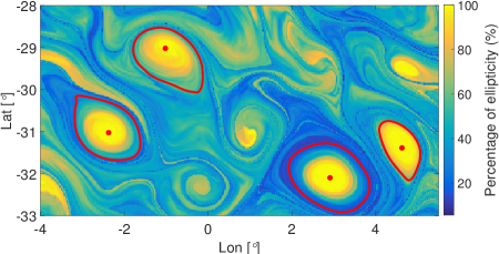
(a)

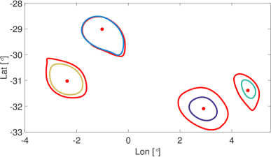
(b)

Figure 16: (a) Ellipticity time field $\tau_{e}(t_{1},t_{0},x_{0})$ for the Agulhas leakage data set of Section 10.6 with $t_{0}=\mathrm{November}\,11,\,2006$ and $t_{1}=t_{0}+90\,\mathrm{days}$. Rotationally coherent Lagrangian vortex boundaries (red) are superimposed for reference. (b) Geodesic vortex boundaries at time $t_{0}$ for the same data set, with the LAVD-based vortex boundaries (red) superimposed.

As seen in Fig. 16a, the pointwise ellipticity time diagnostic highlights the same material vortex regions labelled as coherent by the other two methods. However, it also suggests further vortical regions that are neither rotationally no stretching-wise coherent. The diagnostic does not offer a well-defined boundary for the detected vortices either.

Fig. 16b confirms the expectation that the variationally derived geodesic vortex detection method generally labels the same coherent material vortices, but yields smaller vortex boundaries due to its uniform stretching requirement. This, coupled with the significantly decreased computational cost and coding effort, renders LAVD-based Lagrangian vortex identification preferable over the other two objective methods considered here.

References

- [1] Arnold, V. I. 1978 Ordinary Differential Equations, MIT Press, Cambridge.
- [2] Batchelor, B. G., & Whelan, P.F. 2012 Intelligent Vision Systems for Industry. Springer, London.
- [3] Beal, L. M., De Ruijter, W. P. M., Biastoch, A., Zahn, R. & SCOR/WCRP/IAPSO Working Group 2011 On the role of the Agulhas system in ocean circulation and climate. Nature 472, 429–436.
- [4] Beron-Vera, F. J., Wang, Y., Olascoaga, M. J. , Goni, J. G. & Haller, G. 2013 Objective detection of oceanic eddies and the Agulhas leakage, J. Phys. Oceanogr. 43, 1426–1438.
- [5] Beron-Vera, F. J., Olascoaga, M. J. , Haller, G. Farazmand, M., Triñanes, J., & Wang, Y. 2015 Dissipative inertial transport patterns near coherent Lagrangian eddies in the ocean. Chaos 25, 087412.
- [6] Beron–Vera, F. J. 2015 Flow coherence: Distinguishing cause from effect. in Selected Topics of Computational and Experimental Fluid Mechanics Environmental Science and Engineering (Eds: . Klapp, G. Ruíz Chavarr a, A. M. Ovando, A. López Villa, L. Di G. Sigalotti, Springer, New York. pp: 81-89.
- [7] Bertrand, J. 1873 Théoreme relatif au mouvement d’un point attiré vers un centre fixe. C. R. Acad. Sci. 77, 849–853.
- [8] Blazevski, D., & Haller, G. 2014 Hyperbolic and elliptic transport barriers in three-dimensional unsteady flows. Physica D, 273-274, 46-64.
- [9] Budišić, M., and Mezić, I. 2012 Geometry of the ergodic quotient reveals coherent structures in flows. Physica D., 241, 1255–1269
- [10] Chakraborty, P., Balachandar, S. & Adrian, R. 2005 On the relationships between local vortex identification schemes. J. Fluid Mech. 535, 189–214.
- [11] Chelton, D. B., Gaube, P., Schlax, M. G., Early, J. J., Samelson, R. M. 2011 The influence of nonlinear mesoscale eddies on near-surface oceanic chlorophyll, Science 334, 328–332.
- [12] Chong, M. S., Perry, A. E. & Cantwell, B. J. 1990 A general classification of three-dimensional flow fields. Phys. Fluids A 2, 765–777.
- [13] Cucitore, R., Quadrio, M. & Baron, A. 1999 On the effectiveness and limitations of local criteria for the identification of a vortex. Eur. J. Mech. B/Fluids 18, 261–282.
- [14] Dafermos, C. M. 1971 An invariance principle for compact processes. J. Diff. Eqs. 239-252.
- [15] Dienes, J.K. 1986 A discussion of material rotation and stress rate. Acta Mechanica 65, 1–11.
- [16] Dresselhaus, E. & Tabor, M. 1989 The persistence of strain in dynamical systems. Phys. A: Math. Gen. 22, 971-984
- [17] Dresselhaus, E. & Tabor, M. 1991 The kinematics of stretching and alignment of material elements in general flow fields, Fluid Mech., 236, 415-444.
- [18] Dritschel, D. G. & Waugh, D. W. 1992 Quantification of the inelastic interaction of unequal vortices in two-dimensional vortex dynamics. Phys. Fluids. A 4 (8), 1737-1744.
- [19] Farazmand, M. & Haller, G. 2013 Attracting and repelling Lagrangian coherent structures from a single computation. Chaos 15, 023101 1-11
- [20] Farazmand, M., & Haller, G. 2016 Polar rotation angle identifies elliptic islands in unsteady dynamical systems, Physica D 315 (2016) 1-12.
- [21] Golub, G. H., and Van Loan, C. F. 1983 Matrix Computations, Johns Hopkins University Press, Baltimore, MD.
- [22] Gonzalez, R. C., & Woods, R. E. 2008 Digital Image Processing. Pearson, Prentice Hall.
- [23] Gurtin, M. E. 1982 An Introduction to Continuum Mechanics. Academic Press.
- [24] Hadjighasem, A., and Haller, G. 2016 Geodesic Transport Barriers in Jupiter’s Atmosphere: A Video-Based Analysis, SIAM Review 58(1): 69-89
- [25] Haller, G. 2001 Lagrangian structures and the rate of strain in a partition of two-dimensional turbulence. Phys. Fluids. 13, 3365-3385.
- [26] Haller, G. 2005 An objective definition of a vortex J. Fluid Mech. 525, 1-26.
- [27] Haller, G., & Beron-Vera, F. J. 2013 Coherent Lagrangian vortices: The black holes of turbulence. J. Fluid Mech., 731, R4, 2013.
- [28] Haller, G. 2015 Lagrangian Coherent Structures. Annual Rev. Fluid. Mech, 47, 137-162.
- [29] Haller, G. 2016 Dynamically consistent rotation and stretch tensors from a dynamic polar decomposition. J. Mech. Phys. Solids, 86 (2016) 70-93.
- [30] Helmholtz, H. 1858 Über Integrale der hydrodynamischen Gleichungen, welche den Wirbelbewegungen entsprechen. J. Reine und Angew. Math. 55, 25-55.
- [31] Hunt, J. C. R., Wray, A. A. & Moin, P. 1988 Eddies, stream, and convergence zones in turbulent flows. Center for Turbulence Research Report CTR-S88, pp. 193–208.
- [32] Hussain, A. K. M. F. 1986 Coherent structures and turbulence. J. Fluid Mech. 173, 303–356.
- [33] Ito, M., Yamazaki, T., & Yanagida, M. 2004 On the polar decomposition of the product of two operators and its applications. Integr. Equ. Oper. Theory 49, 461–472.
- [34] Jeong, J. & Hussein, A. K. M. F. 1995 On the identification of a vortex. J. Fluid Mech. 285, 69-94.
- [35] Kevlahan, N. K.-R., & Farge, M. 1997 Vorticity filaments in two-dimensional turbulence: creation, stability and effect. J. Fluid. Mech. 346, 49–76.
- [36] Karrasch, D., Huhn, F., & Haller, G. 2014 Automated detection of coherent Lagrangian vortices in two-dimensional unsteady flows. Proc. Royal Society 471, 20140639
- [37] Lapeyre, G., Klein, P. & Hua, B. L. 1999 Does the tracer gradient vector align with the strain eigenvectors in 2D turbulence? Phys. Fluids 11, 3729–3737.
- [38] Lapeyre, G., Hua, B. L. & Legras, B. 2001 Comment on ”finding finite-time invariant manifolds in two-dimensional velocity fields”. Chaos 11, 427–430.
- [39] Liu, I.-S. 2004 On the transformation property of the deformation gradient under a change of frame. in The Rational Spirit in Modern Continuum Mechanics. C.-S. Man & R. L. Fosdick (eds.) Springer, Amsterdam, 555-562.
- [40] Lugt, H. J. 1972 Vortex Flow in Nature and Technology. Wiley.
- [41] Lugt, H. J. 1979 The dilemma of defining a vortex. In Recent Developments in Theoretical and Experimental Fluid Mechanics. (ed. U. Müller, K. G. Riesner & B. Schmidt), pp. 309–321, Springer.
- [42] Majda, A. J., & Bertozzi, A. L., 2002 Vorticity and Incompressible Flow. Cambridge University Press.
- [43] Mason, E., Pascual, A. & McWilliams, J.C. 2014 A New Sea Surface Height–Based Code for Oceanic Mesoscale Eddy Tracking. J. Atmos. Oceanic Technol., 31, 1181–1188.
- [44] Maxey, M. R. & Riley, J. J. 1983 Equation of motion for a small rigid sphere in a nonuniform flow, Phys. Fluids 26, 883-889.
- [45] Mazloff, M. R., Heimbach, P., & Wunsch, C. 2010 An Eddy-Permitting Southern Ocean State Estimate. J. Phys. Oceanogr. 40, 880-99.
- [46] McWilliams, J. C., 1984 The emergence of isolated coherent vortices in turbulent flow. Fluid Mech. 146, 21-43.
- [47] Milnor, J. 1963 Morse Theory (Based on lecture notes by M. Spivak and R. Wells). Annals of Math. Stud. 51. Princeton University Press, Princeton.
- [48] Öttinger, D., Blazevski, D., & Haller, G. 2015 Global variational approach to elliptic transport barriers in three dimensions. submitted
- [49] Pérez-Muñuzuri, V., & Huhn, F. 2013 Path-integrated Lagrangian measures from the velocity gradient tensor. Nonlin. Processes Geophys., 20, 987–991.
- [50] Provenzale, A. 1999 Transport by coherent barotropic vortices. Annu. Rev. Fluid Mech. 31,55–93.
- [51] Shapiro, A. 1961 Vorticity. US National Committee for Fluid Mechanics Film Series. MIT, Cambridge.
- [52] Smith, A. C., & Kaloni, P.N. 1996 A note on spin, vorticity and the deformation-rate tensor. J. Non-Newtonian Fluid Mech., 62, 95-98
- [53] Tabor, M. & Klapper, I. 1994 Stretching and alignment in chaotic and turbulent flows. Chaos Soliton Fract. 4, 1031–1055.
- [54] Truesdell, C. & Noll, W. 1965 The nonlinear field theories of mechanics, in Handbuch der Physik, Band III/3, e by Flugge, S., (ed.) , Springer-Verlag, Berlin.
- [55] Truesdell, C. & Rajagopal, K. R. 2009 An Introduction to the Mechanics of Fluids. Birkh user, Boston.
- [56] http://www.webbresearch.com/pdf/Apex_Float_Brochure.pdf