Laser-induced electron localization in H${}_{2}^{+}$: Mixed quantum-classical dynamics based on the exact time-dependent potential energy surface

Abstract

We study the exact nuclear time-dependent potential energy surface (TDPES) for laser-induced electron localization with a view to eventually developing a mixed quantum-classical dynamics method for strong-field processes. The TDPES is defined within the framework of the exact factorization [A. Abedi, N. T. Maitra, and E. K. U. Gross, Phys. Rev. Lett. 105, 123002 (2010)] and contains the exact effect of the couplings to the electronic subsystem and to any external fields within a scalar potential. We compare its features with those of the quasistatic potential energy surfaces (QSPES) often used to analyse strong-field processes. We show that the gauge-independent component of the TDPES has a mean-field-like character very close to the density-weighted average of the QSPESs. Oscillations in this component are smoothened out by the gauge-dependent component, and both components are needed to yield the correct force on the nuclei. Once the localization begins to set in, the gradient of the exact TDPES tracks one QSPES and then switches to the other, similar to the description provided by surface-hopping between QSPESs. We show that evolving an ensemble of classical nuclear trajectories on the exact TDPES accurately reproduces the exact dynamics. This study suggests that the mixed quantum-classical dynamics scheme based on evolving multiple classical nuclear trajectories on the exact TDPES will be a novel and useful method to simulate strong field processes.

I Introduction

With the advent of attosecond technology Krausz and Ivanov (2009); Vrakking (2014); Lépine et al. (2014); Haessler et al. (2010); Corkum and Krausz (2007); Calegari et al. (2014), the experimentally accessible time-scale has shifted to that of electronic motion. It allows the observation of electronic motion in real-time, and even offers the control of electron motion and localization via lasers. Several groups Sansone et al. (2010); He et al. (2007); Ray et al. (2009); Singh et al. (2010); Fischer et al. (2010); Calvert et al. (2010); Kelkensberg et al. (2011); He (2012); Liu et al. (2012); Jia et al. (2014); Wang et al. (2015); Kling et al. (2006); Kremer et al. (2009); Roudnev et al. (2004); Tong and Lin (2007); Graefe and Ivanov (2007); Rathje et al. (2013); Kling et al. (2013); Li et al. (2014); Lan et al. (2012) have demonstrated that it is possible to control electronic motion in a dissociating molecule and localize it selectively on one of the products of dissociation, with several different strategies. One technique employs the carrier envelope phase (CEP) of a single few-cycle laser pulse  Kling et al. (2006); Kremer et al. (2009); Roudnev et al. (2004); Tong and Lin (2007); Graefe and Ivanov (2007); Rathje et al. (2013); Kling et al. (2013); Li et al. (2014) , and another employs the time-delay between two coherent ultrashort pulses Sansone et al. (2010); He et al. (2007); Ray et al. (2009); Singh et al. (2010); Fischer et al. (2010); Calvert et al. (2010); Kelkensberg et al. (2011); He (2012); Liu et al. (2012); Jia et al. (2014); Wang et al. (2015).

These experiments so far treat small systems (such as H₂ and D₂), with the aim of understanding the mechanisms of localization, before applying the techniques to the control of larger systems Kübel et al. (2014); Li et al. (2015). Theoretical studies have a dual role Sansone et al. (2010); He et al. (2007); Ray et al. (2009); Singh et al. (2010); Fischer et al. (2010); Calvert et al. (2010); Kelkensberg et al. (2011); He (2012); Liu et al. (2012); Jia et al. (2014); Wang et al. (2015); Kling et al. (2006); Kremer et al. (2009); Roudnev et al. (2004); Tong and Lin (2007); Graefe and Ivanov (2007); Rathje et al. (2013); Kling et al. (2013); Li et al. (2014); Lan et al. (2012) : (i) to help understand the complex correlation between the electron dynamics and nuclear dynamics, and (ii) to establish methods, generally extendable to larger systems, that accurately simulate the coupled electron-nuclear dynamics. For systems with more than two or three degrees of freedom, we must rely on approximate methods, and usually some kind of mixed quantum-classical approach is appropriate, where the electrons are treated quantum-mechanically, coupled to nuclei described via classical trajectories Mitrić et al. (2009); Tavernelli et al. (2010); Richer et al. (2011); Bajo et al. (2012). Different mixed quantum-classical schemes such as Ehrenfest and surface-hopping Tully (1990); Hammes-Schiffer and Tully (1994); Tully (1998), differ in their treatment of the classical nuclear motion, but use the same form for the potential acting on the electrons. For dynamics in strong fields, a surface-hopping scheme between quasi-static potential energy surfaces (QSPES) was introduced Dietrich et al. (1996); Thachuk et al. (1996, 1998), and in fact applied to the electron-localization problem Kelkensberg et al. (2011). Although this semiclassical approach was shown to reproduce the experimental asymmetries reasonably well, it is not altogether clear why surface-hopping should give good predictions, given its problems associated with over-coherence Shenvi et al. (2011); Jasper et al. (2006); Bittner and Rossky (1995); Akimov et al. (2014); Curchod and Tavernelli (2013); Makri (2014); Grunwald et al. (2008); Granucci and Persico (2007).

In this paper, we will study the possibility of using a potential derived from first-principles, the time-dependent potential energy surface (TDPES) Abedi et al. (2010, 2012), in a mixed quantum-classical description of the coupled dynamics. This potential arises out of the exact factorization framework where a time-dependent Schrödinger equation (TDSE) for the nuclei alone can be formulated. The potentials appearing in this equation capture exactly all coupling to the electronic system as well as any external fields, and the resulting nuclear wavefunction reproduces the exact nuclear dynamics. The scalar potential is denoted the TDPES, and in many situations, including all one-dimension problems, the TDPES is the only potential acting on the nuclear subsystem; its gradient therefore yields the exact force on the nuclei. For this reason, it is important to gain an understanding of its structure, to address both points (i) and (ii) above. Therefore, our aim in this paper is to find the exact TDPES for the problem of laser-induced electron localization in a one-dimensional model of H${}_{2}^{+}$, compare its structure with potential surfaces more traditionally used for strong-field dynamics, and study classical nuclear dynamics on the exact TDPES with a view to developing mixed quantum-classical schemes based on the exact factorization.

Previous work Abedi et al. (2013); Agostini et al. (2013, 2015) has analysed the structure of the exact TDPES for a case of field-free dynamics, non-adiabatic charge-transfer in the Shin-Metiu model Shin and Metiu (1995), finding that much intuition is gained by analysing it in term of the Born-Oppenheimer (BO) potential energy surfaces (BOPESs), and that such an analysis enables connections to be made with traditional approximate methods for coupled electron-ion dynamics, such as surface-hopping. Further, it was found that evolving an ensemble of classical nuclear trajectories on the exact TDPES accurately reproduces the exact nuclear dynamics Agostini et al. (2015).

We will show here that analogous conclusions can be drawn for the laser-induced electron localization problem: an ensemble of classical nuclear trajectories evolving on the exact TDPES accurately reproduces the exact nuclear dynamics, and analysis in terms of the QSPESs, which play the role of the BOPESs when strong fields are present, is helpful. The TDPES naturally separates into a gauge-independent part and a gauge-dependent part. We show that the density-weighted average of the QSPESs approximates the gauge-independent component, which is rather oscillatory and the force on the nuclei resulting from its gradient is incorrect. Once the gauge-dependent component of the TDPES is included, the oscillations smoothen out: together, they yield the correct force on the nuclei. Further, we find that, once localization begins to set in, the gradient of the exact TDPES at the location of the mean nuclear position, tracks that of one QSPES and then switches to the other, resembling the picture provided by the semiclassical surface-hopping approach Kelkensberg et al. (2011); Thachuk et al. (1996, 1998).

A multiple trajectory Ehrenfest dynamics simulation shows that although the nuclear dynamics is reasonably reproduced, an incorrect electron localization asymmetry is obtained. The error can be related to the incorrect BO projections of the electronic wavefunction. The fact that the Ehrenfest dynamics yields inaccurate electron dynamics can be anticipated from our recent work on the exact electronic-TDPES Suzuki et al. (2014): in this complementary picture, instead of asking what is the exact potential acting on nuclei in an exact TDSE for nuclei, one asks what is the exact potential acting on electrons in an exact TDSE for the electronic subsystem. We found Suzuki et al. (2014) that the exact electronic-TDPES is significantly different from the potential acting on electrons in the usual mixed quantum-classical schemes – including Ehrenfest as well as surface-hopping schemes – yielding significant errors in the prediction of the electron localization asymmetry. The results of the present paper suggest that, instead, mixed quantum-classical schemes based on evolving multiple classical trajectories on the exact TDPES (or good approximations to it) will be a useful method to simulate strong field processes.

This paper is organized as follows. In section II, we review two different concepts of potential energy surfaces for TD processes in laser fields: the QSPES and the exact TDPES. In section III we compare the features of these potentials for electron localization dynamics in the dissociation of a model H${}_{2}^{+}$ molecule induced by time-delayed coherent ultra shortlaser pulses. We show the exact TDPES gives the correct force acting on nuclei, so evolving multiple classical trajectories on it reproduces the correct nuclear wavepacket dynamics. The force obtained from surface-hopping between QSPESs can approximately reproduce such an exact force once localization begins to set in. We also compute multiple trajectory Ehrenfest dynamics and reveal how it fails to reproduce electron localization dynamics while it reasonably reproduces the nuclear dynamics. In section IV we summarize the results and remark on the future directions.

II THEORY

II.1 Quasi-static potential energy surface

In this section we first review the concept of the QSPES introduced for the description of molecules in strong-fields. The QSPES has been thoroughly discussed in earlier works Kelkensberg et al. (2011); Dietrich and Corkum (1992); Zuo and Bandrauk (1995); Seideman et al. (1995); Dietrich et al. (1996); Thachuk et al. (1996, 1998); Kawata et al. (1998, 1999); Kono et al. (2004); Kato et al. (2009) , but we here give a discussion particularly relevant for the electron localization dynamics problem in the dissociation of H${}_{2}^{+}$.

For this problem, the essential physics is contained in the two lowest field-free electronic states of the BO Hamiltonian, i.e., the 1s$\sigma_{g}$ and 2p$\sigma_{u}$ states, and the full molecular wavefunction $\Psi(R,{\bf r},t)$ of the system can be expressed as

$$\Psi(R,{\bf r},t)=\chi_{g}(R,t)\phi^{g}_{R}({\bf r})+\chi_{u}(R,t)\phi^{u}_{R}({\bf r})\;.$$ (1)

Here $\chi_{g}(R,t)$ and $\chi_{u}(R,t)$ describe nuclear wavefunctions that exist in the 1s$\sigma_{g}$ and 2p$\sigma_{u}$ states respectively, functions of the internuclear distance $R$ and time $t$, and $\phi^{g}_{R}({\bf r})$ and $\phi^{u}_{R}({\bf r})$ describe the 1s$\sigma_{g}$ and 2p$\sigma_{u}$ electronic wavefunction respectively, which parametrically depend on $R$. Since $\phi^{g}_{R}({\bf r})$ and $\phi^{u}_{R}({\bf r})$ are bonding and anti-bonding combination of 1s atomic orbitals, a coherent superposition of them provides the localized electronic states $\phi^{\rm left,right}_{R}({\bf r})=\frac{1}{\sqrt{2}}(\phi^{g}_{R}({\bf r})\pm\phi^{u}_{R}({\bf r}))$ that have the electron on either the left or the right proton. These states form a convenient basis in which to monitor the electron localization asymmetry. In the experiment, interactions of the molecule with the time-delayed infra-red laser field in the course of the dissociation provides a coupling of $\phi^{g}_{R}({\bf r})$ and $\phi^{u}_{R}({\bf r})$, creating a coherent superposition state, and, instead of Eq. 1, it is instructive to write:

$$\Psi(R,{\bf r},t)=\chi_{\rm left}(R,t)\phi^{\rm left}_{R}({\bf r})+\chi_{\rm right}(R,t)\phi^{\rm right}_{R}({\bf r})$$ (2)

where $\chi_{\rm left}(R,t)$ and $\chi_{\rm right}(R,t)$ are defined as the nuclear wavefunctions that exist in connection with $\phi^{\rm left}_{R}({\bf r})$ and $\phi^{\rm right}_{R}({\bf r})$. Measurements of ion fragment asymmetries left or right along the polarization axis directly relate to $\chi_{\rm left}(R,t)$ and $\chi_{\rm right}(R,t)$.

While the field-free states above are useful to analyse the asymmetry, to understand the time-development of the localization it is helpful to consider a third, time-dependent, basis, the TD quasistatic states, $\phi^{\rm QS(i)}_{R}({\bf r},t)$, also known as phase-adiabatic states. These states are defined as instantaneous eigenstates of the instantaneous electronic Hamiltonian $\hat{H}^{\rm int}_{R}({\bf r},t)$, defined by

$$\hat{H}^{\rm int}_{R}({\bf r},t)=\hat{H}^{\rm BO}_{R}({\bf r})+\hat{v}_{\rm laser}({\bf r},t),$$ (3)

i.e.,

$$\hat{H}^{\rm int}_{R}({\bf r},t)\phi^{\rm QS(i)}_{R}({\bf r},t)=\epsilon^{\rm QS(i)}(R,t)\phi^{\rm QS(i)}_{R}({\bf r},t)$$ (4)

where $\epsilon^{\rm QS(i)}(R,t)$ are the quasistatic potential energy surfaces (QSPESs). Within our two-state model we may write

$$\phi^{\rm QS(i)}_{R}({\bf r},t)=c_{g}^{(i)}(R,t)\phi^{g}_{R}({\bf r})+c_{u}^{(i)}(R,t)\phi^{u}_{R}({\bf r}),$$ (5)

so that the $\epsilon^{\rm QS(i)}(R,t)$ of Eq. (4) are given by the eigenvalue equation:

$$\left(\begin{array}[]{cc}\langle\phi^{g}_{R}\arrowvert\hat{H}^{\rm int}_{R}\arrowvert\phi^{g}_{R}\rangle&\langle\phi^{g}_{R}\arrowvert\hat{H}^{\rm int}_{R}\arrowvert\phi^{u}_{R}\rangle\\ \langle\phi^{u}_{R}\arrowvert\hat{H}^{\rm int}_{R}\arrowvert\phi^{g}_{R}\rangle&\langle\phi^{u}_{R}\arrowvert\hat{H}^{\rm int}_{R}\arrowvert\phi^{u}_{R}\rangle\end{array}\right)\left(\begin{array}[]{cc}c_{g}^{(i)}\\ c_{u}^{(i)}\end{array}\right)=\epsilon^{\rm QS(i)}\left(\begin{array}[]{cc}c_{g}^{(i)}\\ c_{u}^{(i)}\end{array}\right).$$ (6)

Therefore we can express the QSPESs in terms of the BOPESs $\epsilon^{\rm BO(i)}(R)$ as

$$\begin{split}\epsilon^{\rm QS(1,2)}(R,t)=&\epsilon^{\rm BO(1,2)}(R)\cos^{2}\theta(R,t)+\epsilon^{\rm BO(2,1)}(R)\sin^{2}\theta(R,t)\\ &\pm\langle\phi^{g}_{R}\arrowvert\hat{v}_{\rm laser}\arrowvert\phi^{u}_{R}\rangle\sin 2\theta(R,t)\end{split}$$ (7)

and the electronic quasi-static eigenstates in terms of the BO states,

$$\begin{split}&\phi^{\rm QS(1)}_{R}({\bf r},t)=\cos\theta(R,t)\phi^{g}_{R}({\bf r})+\sin\theta(R,t)\phi^{u}_{R}({\bf r})\\ &\phi^{\rm QS(2)}_{R}({\bf r},t)=\sin\theta(R,t)\phi^{g}_{R}({\bf r})-\cos\theta(R,t)\phi^{u}_{R}({\bf r}),\end{split}$$ (8)

where the TD mixing parameter $\theta(R,t)$ is given by

$$\tan 2\theta(R,t)=\frac{2\langle\phi^{g}_{R}\arrowvert\hat{v}_{\rm laser}\arrowvert\phi^{u}_{R}\rangle}{\epsilon^{\rm BO(1)}(R)-\epsilon^{\rm BO(2)}(R)}.$$ (9)

The molecular wavefunction expressed in terms of quasi-static states is

$$\Psi(R,{\bf r},t)=\chi^{\rm QS}_{1}(R,t)\phi^{\rm QS(1)}_{R}({\bf r},t)+\chi^{\rm QS}_{2}(R,t)\phi^{\rm QS(2)}_{R}({\bf r},t).$$ (10)

Note that the nuclear wavefunctions $\chi^{\rm QS}_{1}(R,t)$ and $\chi^{\rm QS}_{2}(R,t)$ that are connected to the quasi-static states $\phi^{\rm QS(1)}_{R}({\bf r},t)$ and $\phi^{\rm QS(2)}_{R}({\bf r},t)$ can be expressed in terms of $\chi_{\rm left}(R,t)$ and $\chi_{\rm right}(R,t)$ as

$$\begin{split}\chi^{\rm QS}_{1}(R,t)=&\frac{1}{\sqrt{2}}[\chi_{\rm left}(R,t)(\cos\theta+\sin\theta)\\ &+\chi_{\rm right}(R,t)(\cos\theta-\sin\theta)]\\ \chi^{\rm QS}_{2}(R,t)=&\frac{1}{\sqrt{2}}[\chi_{\rm left}(R,t)(-\cos\theta+\sin\theta)\\ &+\chi_{\rm right}(R,t)(\cos\theta+\sin\theta)].\end{split}$$ (11)

which can be used to extract the electron localization from $\chi^{\rm QS}_{1}(R,t)$ and $\chi^{\rm QS}_{2}(R,t)$.

A semi-classical surface-hopping model based on QSPESs has recently been utilized to understand and reproduce the electron localization dynamics and asymmetry Kelkensberg et al. (2011); Thachuk et al. (1996, 1998) in H${}_{2}^{+}$. In this approach, an ensemble of classical nuclear trajectories evolve on one QSPES or the other QSPES, making instantaneous hops between them as determined by a Landau-Zener formula. It was shown that the electron localization sets in a region where the dynamics is intermediate between adiabatic and diabatic: the ensemble of nuclear trajectories traverses several laser-induced avoided crossings between the QSPESs. This semi-classical method gives asymmetry parameters in reasonably good overall agreement with that obtained from the full TDSE although the details differ. The agreement lends some hope to the use of this semiclassical scheme to simulate coupled electron-ion dynamics in control problems in more complicated systems; however, at the same time a further understanding of the errors in the details is desirable. We will analyse this approach by comparing the QSPESs with the exact TDPES, which we will review in the next section.

II.2 Exact time-dependent potential energy surface

In Ref. Abedi et al. (2010, 2012), it was shown that the full molecular wavefunction $\Psi({\underline{\underline{\bf r}}},{\underline{\underline{\bf R}}},t)$ which solves the TDSE

$$\hat{H}\Psi({\underline{\underline{\bf r}}},{\underline{\underline{\bf R}}},t)=i\partial_{t}\Psi({\underline{\underline{\bf r}}},{\underline{\underline{\bf R}}},t)$$ (12)

can be exactly factorized to the single product

$$\Psi({\underline{\underline{\bf r}}},{\underline{\underline{\bf R}}},t)=\chi({\underline{\underline{\bf R}}},t)\Phi_{\underline{\underline{\bf R}}}({\underline{\underline{\bf r}}},t)$$ (13)

of the nuclear wavefunction $\chi({\underline{\underline{\bf R}}},t)$ and the electronic wavefunction $\Phi_{\underline{\underline{\bf R}}}({\underline{\underline{\bf r}}},t)$ that parametrically depends on the nuclear positions ${\underline{\underline{\bf R}}}$ and satisfies the partial normalization condition

$$\int d{\underline{\underline{\bf r}}}|\Phi_{\underline{\underline{\bf R}}}({\underline{\underline{\bf r}}},t)|^{2}=1\;\;\;\;\forall{\underline{\underline{\bf R}}},t.$$ (14)

Here, the complete molecular Hamiltonian is

$$\hat{H}=\hat{T}_{n}({\underline{\underline{\bf R}}})+\hat{V}^{n}_{ext}({\underline{\underline{\bf R}}},t)+\hat{H}_{\rm BO}({\underline{\underline{\bf r}}},{\underline{\underline{\bf R}}})+\hat{v}^{e}_{ext}({\underline{\underline{\bf r}}},t),$$ (15)

and $\hat{H}_{\rm BO}({\underline{\underline{\bf r}}},{\underline{\underline{\bf R}}})$ is the BO electronic Hamiltonian,

$$\hat{H}_{\rm BO}=\hat{T}_{e}({\underline{\underline{\bf r}}})+\hat{W}_{ee}({\underline{\underline{\bf r}}})+\hat{W}_{en}({\underline{\underline{\bf r}}},{\underline{\underline{\bf R}}})+\hat{W}_{nn}({\underline{\underline{\bf R}}}).$$ (16)

Note that $\hat{T}_{n}=-\sum_{\alpha=1}^{N_{n}}\frac{\nabla^{2}_{\alpha}}{2M_{\alpha}}$ and $\hat{T}_{e}=-\sum_{j=1}^{N_{e}}\frac{\nabla^{2}_{j}}{2m}$ are the nuclear and electronic kinetic energy operators, $\hat{W}_{ee}$, $\hat{W}_{en}$ and $\hat{W}_{nn}$ are the electron-electron, electron-nuclear and nuclear-nuclear interaction, and $\hat{V}^{n}_{ext}({\underline{\underline{\bf R}}},t)$ and $\hat{v}^{e}_{ext}({\underline{\underline{\bf r}}},t)$ are time-dependent (TD) external potentials acting on the nuclei and electrons, respectively. Throughout this paper ${\underline{\underline{\bf R}}}$ and ${\underline{\underline{\bf r}}}$ collectively represent the nuclear and electronic coordinates respectively and $\hbar=1$.

Returning to Eq. (13), the stationary variations of the quantum mechanical action with respect to $\Phi_{\underline{\underline{\bf R}}}({\underline{\underline{\bf r}}},t)$ and $\chi({\underline{\underline{\bf R}}},t)$ under the condition (14) lead to the following equations of motion for $\chi({\underline{\underline{\bf R}}},t)$ and $\Phi_{\underline{\underline{\bf R}}}({\underline{\underline{\bf r}}},t)$:

$$\begin{split}\left(\hat{H}_{BO}({\underline{\underline{\bf r}}},{\underline{\underline{\bf R}}})+\hat{v}^{e}_{ext}({\underline{\underline{\bf r}}},t)+\hat{U}_{en}^{coup}[\Phi_{\underline{\underline{\bf R}}},\chi]-\epsilon({\underline{\underline{\bf R}}},t)\right)\Phi_{{\underline{\underline{\bf R}}}}({\underline{\underline{\bf r}}},t)\\ =i\partial_{t}\Phi_{{\underline{\underline{\bf R}}}}({\underline{\underline{\bf r}}},t)\end{split}$$ (17)

$$\begin{split}\left[\sum_{\alpha=1}^{N_{n}}\frac{\left[-i\nabla_{\alpha}+{\bf A}_{\alpha}({\underline{\underline{\bf R}}},t)\right]^{2}}{2M_{\alpha}}+\hat{V}^{n}_{ext}({\underline{\underline{\bf R}}},t)+\epsilon({\underline{\underline{\bf R}}},t)\right]\chi({\underline{\underline{\bf R}}},t)\\ =i\partial_{t}\chi({\underline{\underline{\bf R}}},t).\end{split}$$ (18)

Here, $\epsilon({\underline{\underline{\bf R}}},t)$ is the exact nuclear TDPES

$$\epsilon({\underline{\underline{\bf R}}},t)=\left\langle\Phi_{\underline{\underline{\bf R}}}(t)\right|\hat{H}_{BO}+\hat{v}^{e}_{ext}({\underline{\underline{\bf r}}},t)+\hat{U}_{en}^{coup}-i\partial_{t}\left|\Phi_{\underline{\underline{\bf R}}}(t)\right\rangle_{\underline{\underline{\bf r}}},$$ (19)

$\hat{U}_{en}^{coup}[\Phi_{\underline{\underline{\bf R}}},\chi]$ is the “electron-nuclear coupling operator”,

$$\hat{U}_{en}^{coup} [\Phi_{\underline{\underline{\bf R}}},\chi]=\sum_{\alpha=1}^{N_{n}}\frac{1}{M_{\alpha}}\left[\frac{\left[-i\nabla_{\alpha}-{\bf A}_{\alpha}({\underline{\underline{\bf R}}},t)\right]^{2}}{2}\right.$$ (20)

$$\left.+\left(\frac{-i\nabla_{\alpha}\chi}{\chi}+{\bf A}_{\alpha}({\underline{\underline{\bf R}}},t)\right)\left(-i\nabla_{\alpha}-{\bf A}_{\alpha}({\underline{\underline{\bf R}}},t)\right)\right],$$

and ${\bf A}_{\alpha}\left({\underline{\underline{\bf R}}},t\right)$ is the TD vector potential potential,

$${\bf A}_{\alpha}\left({\underline{\underline{\bf R}}},t\right)=\left\langle\Phi_{\underline{\underline{\bf R}}}(t)\right|-i\nabla_{\alpha}\left.\Phi_{\underline{\underline{\bf R}}}(t)\right\rangle_{\underline{\underline{\bf r}}}.$$ (21)

The symbol $\left\langle\,\,\cdot\,\,\right\rangle_{\underline{\underline{\bf r}}}$ indicates an integration over electronic coordinates only. Note that the PNC makes the factorization (13) unique up to within a $({\underline{\underline{\bf R}}},t)$-dependent gauge transformation,

$$\begin{array}[]{rcl}\chi({\underline{\underline{\bf R}}},t)\rightarrow\tilde{\chi}({\underline{\underline{\bf R}}},t)&=&e^{-i\theta({\underline{\underline{\bf R}}},t)}\chi({\underline{\underline{\bf R}}},t)\\ \Phi_{\underline{\underline{\bf R}}}({\underline{\underline{\bf r}}},t)\rightarrow\tilde{\Phi}_{\underline{\underline{\bf R}}}({\underline{\underline{\bf r}}},t)&=&e^{i\theta({\underline{\underline{\bf R}}},t)}\Phi_{\underline{\underline{\bf R}}}({\underline{\underline{\bf r}}},t),\end{array}$$ (22)

and Eqs. (17) and (18) are form invariant under this transformation while the scalar potential and the vector potential transform as

$$\tilde{\epsilon}({\underline{\underline{\bf R}}},t) = \epsilon({\underline{\underline{\bf R}}},t)+\partial_{t}\theta({\underline{\underline{\bf R}}},t)$$ (23)

$$\tilde{\bf A}_{\alpha}({\underline{\underline{\bf R}}},t) = {\bf A}_{\alpha}({\underline{\underline{\bf R}}},t)+\nabla_{\alpha}\theta({\underline{\underline{\bf R}}},t).$$ (24)

The equation for the exact nuclear wavefunction, Eq. (18), is Schrödinger-like, and the TD vector potential (21) and TD scalar potential (19) that appear in it, exactly govern the nuclear dynamics. It is important to note that $\chi({\underline{\underline{\bf R}}},t)$ can be interpreted as the exact nuclear wave-function since it leads to an $N$-body nuclear density, $\Gamma({\underline{\underline{\bf R}}},t)=|\chi({\underline{\underline{\bf R}}},t)|^{2},$ and an $N$-body current density, ${\bf J}_{\alpha}({\underline{\underline{\bf R}}},t)=\frac{1}{M_{\alpha}}\Big{[}\mbox{Im}(\chi^{*}({\underline{\underline{\bf R}}},t)\nabla_{\alpha}\chi({\underline{\underline{\bf R}}},t))+\Gamma({\underline{\underline{\bf R}}},t){\bf A}_{\alpha}({\underline{\underline{\bf R}}},t)\Big{]},$ which reproduce the true nuclear $N$-body density and current density Abedi et al. (2012) obtained from the full wave-function $\Psi({\underline{\underline{\bf r}}},{\underline{\underline{\bf R}}},t)$.

In our previous work the shape of this exact TDPES has been useful to interpret dynamics for both a strong field process (strong-field dissociation of H${}_{2}^{+}$) Abedi et al. (2010, 2012) as well as for field-free dynamics of non-adiabatic charge-transfer Abedi et al. (2013); Agostini et al. (2013, 2015). In particular, in the field-free case, a detailed study of the form of its gauge-dependent and gauge-independent parts proved instructive to understand its effect on the nuclear dynamics, and the structure to be expected for general field-free problems. Importantly, in a mixed quantum-classical description, the gradient of this exact TDPES gives uniquely the correct force on the nuclei, and it was shown, in the field-free case, that an ensemble of classical trajectories evolving on the exact TDPES accurately reproduces the exact nuclear wavepacket dynamics. We now consider a detailed study of the form of the exact TDPES for the present case of dynamics in external fields, with the aims of addressing three questions. First, does running classical nuclear dynamics on the exact TDPES reproduce the dynamics of laser-induced electron localization? Second, how are the QSPESs related to the exact TDPES? Third, can we see hints of the semiclassical surface-hopping method in the exact TDPES?

III Results and discussion

III.1 Theoretical model

We employ a one-dimensional model of the H${}_{2}^{+}$ molecule to study electron localization dynamics achieved by time-delayed coherent ultra short laser pulses Sansone et al. (2010); He et al. (2007); Kelkensberg et al. (2011). In the experiment, first an ultraviolet (UV) pulse excites H${}_{2}^{+}$ to the dissociative 2p$\sigma_{u}$ state while a second time-delayed infrared (IR) pulse induces electron transfer between the dissociating atoms. In our model, we start the dynamics after the excitation by the UV pulse: the wavepacket starts at $t=0$ on the first excited state (2p$\sigma_{u}$ state) of H${}_{2}^{+}$ as a Frank-Condon projection of the wavefunction of the ground state, and then is exposed to the IR laser pulse. The full Hamiltonian of the system is given by

$$\begin{split}&\hat{H}(R,z,t)=\hat{T}_{n}(R)+\hat{H}^{\rm int}_{R}(z,t)\\ &=\hat{T}_{n}(R)+\hat{T}_{e}(z)+\hat{W}_{nn}(R)+\hat{W}_{en}(z,R)+\hat{v}_{\rm laser}(z,t)\end{split}$$ (25)

where $R$ is the internuclear distance and $z$ is the electronic coordinate as measured from the nuclear center of mass. The kinetic energy terms are $\hat{T}_{n}(R)=-\frac{1}{2\mu_{n}}\frac{\partial^{2}}{\partial R^{2}}$ and, $\hat{T}_{e}(z)=-\frac{1}{2\mu_{e}}\frac{\partial^{2}}{\partial z^{2}}$, respectively, where the reduced mass of the nuclei is given by $\mu_{n}=M_{\rm H}/2$, and reduced electronic mass is given by $\mu_{e}=\frac{2M_{\rm H}}{2M_{\rm H}+1}$ ($M_{\rm H}$ is the proton mass). The interactions are soft-Coulomb: $\hat{W}_{nn}(R)=\frac{1}{\sqrt{0.03+R^{2}}}$, and $\hat{W}_{en}(z,R)=-\frac{1}{\sqrt{1.0+(z-\frac{R}{2})^{2}}}-\frac{1}{\sqrt{1.0+(z+\frac{R}{2})^{2}}}$ (and $\hat{W}_{ee}=0$). The IR pulse is described within the dipole approximation and length gauge, as $\hat{v}^{e}_{ext}(z,t)=E(t)q_{e}z$, where $E(t)=E_{0}\exp\left[-\left(\frac{t-\Delta t}{\tau}\right)^{2}\right]\cos(\omega(t-\Delta t))$, and the reduced charge $q_{e}=\frac{2M_{\rm H}+2}{2M_{\rm H}+1}$. The wavelength is 800 nm and the peak intensity $I_{0}=E_{0}^{2}=3.0\times 10^{12}$W/cm². The pulse duration is $\tau=4.8fs$ and $\Delta t$ is the time delay between the UV and IR pulses. Here we show the results of $\Delta t=$ 7 fs.

We propagate the full TDSE

$$\hat{H}(z,R,t)\Psi(z,R,t)=i\partial_{t}\Psi(z,R,t)$$ (26)

numerically exactly to obtain the full molecular wavefunction $\Psi(z,R,t)$, and from it we calculate the probabilities of directional localization of the electron, $P_{\pm}$, which are defined as $P_{+(-)}=\int_{z>(<)0}dz\int dR|\Psi(z,R,t)|^{2}$. These are shown as the green solid ($P_{-}$) and red dashed ($P_{+}$) lines in Fig. 1b. It is evident from this figure that considerable electron localization occurs, with the electron density predominantly localized on the left (negative z-axis).

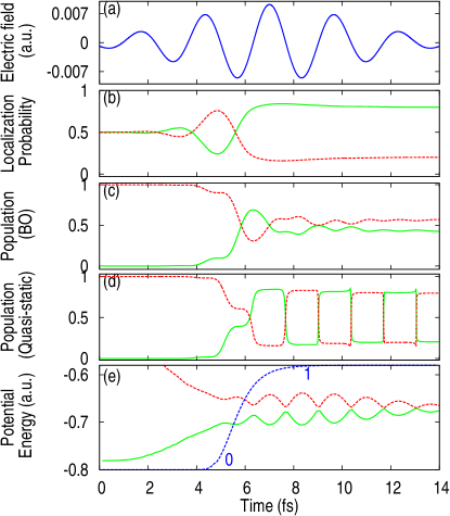
Figure 1: (a) 4.8 fs FWHM 800 nm laser pulse. (b) Electron localization probabilities along the negative (green solid line) and the positive z-axis (red dashed line) as a function of time. (c) Population dynamics during dissociation on the BO state $\phi^{g}_{R}(z)$ (green solid) and $\phi^{u}_{R}(z)$ (red dashed). (d) Population dynamics during dissociation on the 1st quasi-static state $\phi^{\rm QS(1)}_{R}(z,t)$ (green solid) and 2nd quasi-static state $\phi^{\rm QS(2)}_{R}(z,t)$ (red dashed). (e) Quasi-static potential energy surfaces $\epsilon^{\rm QS(1)}(R,t)$ (green solid) and $\epsilon^{\rm QS(2)}(R,t)$ (red dashed) for a nuclear trajectory $\langle R\rangle(t)$ that tracks the expectation value of the internuclear distance. The blue curve shows the transition probability given by a Landau-Zener formula  (Eq. 18 of Ref. Kelkensberg et al. (2011)).

Furthermore, we calculate the population dynamics of the BO states $\phi^{g}_{R}(z)$ (green solid) and $\phi^{u}_{R}(z)$ (red dashed) (Fig. 1c) during dissociation, as well as the population dynamics on the 1st quasi-static state $\phi^{\rm QS(1)}_{R}(z,t)$ (green solid) and 2nd quasi-static state $\phi^{\rm QS(2)}_{R}(z,t)$ (red dashed) (Fig. 1d); the relative simplicity of the latter demonstrate the usefulness of the QS basis for laser-induced processes. We then plot the QSPESs $\epsilon^{\rm QS(1)}(\langle R(t)\rangle,t)$ (green solid) and $\epsilon^{\rm QS(2)}(\langle R(t)\rangle,t)$ (red dashed) evaluated at a nuclear trajectory $\langle R(t)\rangle$ that tracks the expectation value of the internuclear distance. These results coincide qualitatively with the previous results reported by Kelkensberg et al. Kelkensberg et al. (2011) Panels b, d, and e, suggest that the electron localization is determined by the passage of the dissociating molecule through a regime where the laser-molecule interaction is neither diabatic nor adiabatic. As discussed in the previous section, the semiclassical scheme, with the avoided crossings between the QSPES inducing the trajectories to hop between them, reproduces the general behavior. Next, we will compare the exact TDPES with the QSPES to understand the relation between the two, shed some light on the surface-hopping scheme, and find the exact force on classical nuclei.

III.2 Exact TDPES vs. QSPES

First we show the exact TDPES for this process in Fig. 2. We calculate the TDPES in the gauge where the vector potential $A(R,t)$ is zero Abedi et al. (2012), so the TDPES $\epsilon(R,t)$ is the only potential acting on the nuclear subsystem. It is instructive to express the TDPES as the sum of the gauge-independent term $\epsilon_{gi}(R,t)$ and the gauge-dependent term $\epsilon_{gd}(R,t)$ as done in previous studies Abedi et al. (2012, 2013) :

$$\epsilon(R,t)=\epsilon_{gi}(R,t)+\epsilon_{gd}(R,t)$$ (27)

where

$$\epsilon_{gi}(R,t)=\left\langle\Phi_{R}(t)\right|\hat{H}_{BO}+\hat{v}_{\rm laser}+\hat{U}_{en}^{coup}\left|\Phi_{R}(t)\right\rangle_{z}$$ (28)

and

$$\epsilon_{gd}(R,t)=\left\langle\Phi_{R}(t)\right|-i\partial_{t}\left|\Phi_{R}(t)\right\rangle_{z}.$$ (29)

In Fig. 2, $\epsilon(R,t)$(black solid), $\epsilon_{gi}(R,t)$(blue solid) and $\epsilon_{gd}(R,t)$(orange solid) are plotted at nine different times, along with the two lowest BOPESs, $\epsilon^{\rm BO(1)}(R)$ and $\epsilon^{\rm BO(2)}(R)$. (Note that the TDPES $\epsilon(R,t)$(black solid) and its GD component $\epsilon_{gd}(R,t)$(orange solid) have been rigidly shifted along the energy axis).

We also plot the exact nuclear density $|\chi(R,t)|^{2}$ (green solid) and the nuclear density reconstructed from evolving an ensemble of $800$ classical trajectories on the exact TDPES (red dashed) Agostini et al. (2015) at each time. The closeness of these last two curves shows that a mixed quantum-classical scheme for the electron localization process is appropriate and that the exact TDPES $\epsilon(R,t)$ gives the correct force acting on classical nuclei in such a scheme.

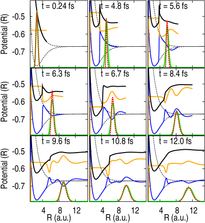
Figure 2: Snapshot of the exact TDPES $\epsilon(R,t)$ (black solid) , its gauge-invariant part $\epsilon_{gi}(R,t)$ (blue solid) and gauge-dependent part $\epsilon_{gd}(R,t)$ (orange solid) at indicated times along with two lowest BOPESs (black dashed). Furthermore, the exact nuclear density $|\chi(R,t)|^{2}$ (green solid) and the nuclear density reconstructed from the multiple trajectory dynamics on the exact TDPES (red dashed) for each time are also plotted.

In previous work Abedi et al. (2013); Agostini et al. (2013, 2015), step-like features of $\epsilon_{gi}(R,t)$ and $\epsilon_{gd}(R,t)$ in the field-free non-adiabatic process in the vicinity of the avoided crossing have been shown. In particular, after passage through the avoided crossing, where the nuclear wavepacket had spatially separated on two BOPESs, the GI component tracked one BO surface or the other, with a step between them, while the GD component was piecewise flat, but with a step in the same region with opposite sign. The net TDPES was overall more smooth than either of the components. Here, we find again very interesting features of $\epsilon_{gi}(R,t)$ and $\epsilon_{gd}(R,t)$. First note that both $\epsilon_{gi}(R,t)$ and $\epsilon_{gd}(R,t)$ shows many small hills and valleys after the laser-induced nonadiabatic transitions begin, but with opposite slopes to each other, so that these structures largely cancel each other when the exact TDPES $\epsilon(R,t)$ is constructed (much like the near-cancellation of the steps in the field-free case). Like the field-free case, both the GI and GD terms are important to consider to predict the correct nuclear dynamics. Second, in the present strong-field case, unlike the field-free examples studied in Abedi et al. (2013); Agostini et al. (2013, 2015), $\epsilon_{gi}(R,t)$ does not piecewise track one BOPES or the other. However, it does track a density-weighted QSPES, as we will show next.

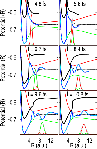
Figure 3: Snapshots of the gauge-invariant part of exact TDPES $\epsilon_{gi}(R,t)$ (blue solid), QSPESs $\epsilon^{\rm QS(1)}(R,t)$ (green solid) and $\epsilon^{\rm QS(2)}(R,t)$ (red solid), and the weighted average of the QSPESs $\epsilon^{\rm QS}_{ave}(R,t)$ (light blue solid) at indicated times. $|\chi^{\rm QS}_{1}(R,t)|^{2}$ (green) and $|\chi^{\rm QS}_{2}(R,t)|^{2}$ (red) are also plotted.

In Fig. 3, we show $\epsilon(R,t)$(black solid) (which is again rigidly shifted along the energy axis) and the gauge-invariant part $\epsilon_{gi}(R,t)$ (blue solid) together with the QSPESs $\epsilon^{\rm QS(1)}(R,t)$ (green solid) and $\epsilon^{\rm QS(2)}(R,t)$ (red solid). We find that the oscillations in the gauge-invariant part of exact TDPES $\epsilon_{gi}(R,t)$ (blue solid) tend to step between the two QSPESs: $|\chi^{\rm QS}_{1}(R,t)|^{2}$ and $|\chi^{\rm QS}_{2}(R,t)|^{2}$ are also plotted in Fig. 3, and we see that $\epsilon_{gi}(R,t)$ tends towards the QSPES whose population is dominant, i.e. when $|\chi^{\rm QS}_{1}(R,t)|^{2}$ is larger than $|\chi^{\rm QS}_{2}(R,t)|^{2}$ $\epsilon_{gi}(R,t)$ approaches to $\epsilon^{\rm QS(1)}(R,t)$ and when $|\chi^{\rm QS}_{2}(R,t)|^{2}$ is larger than $|\chi^{\rm QS}_{1}(R,t)|^{2}$ $\epsilon_{gi}(R,t)$ approaches to $\epsilon^{\rm QS(2)}(R,t)$. In fact, $\epsilon_{gi}(R,t)$ lies practically on top of the the weighted average of the quasi-static surfaces $\epsilon^{\rm QS}_{ave}(R,t)$:

$$\begin{split}\epsilon^{\rm QS}_{ave}(R,t)&=\frac{|\chi^{\rm QS}_{1}(R,t)|^{2}}{|\chi^{\rm QS}_{1}(R,t)|^{2}+|\chi^{\rm QS}_{2}(R,t)|^{2}}\epsilon^{\rm QS(1)}(R,t)\\ &+\frac{|\chi^{\rm QS}_{2}(R,t)|^{2}}{|\chi^{\rm QS}_{1}(R,t)|^{2}+|\chi^{\rm QS}_{2}(R,t)|^{2}}\epsilon^{\rm QS(2)}(R,t)\end{split}$$ (30)

This is plotted with light blue line in Fig. 3. Therefore the weighted-average of the QSPESs approximates the gauge-invariant part of exact TDPES $\epsilon_{gi}(R,t)$, but not the full exact TDPES $\epsilon(R,t)$. In fact, this is quite analogous to the previous results on the field-free passage through an avoided crossing Abedi et al. (2013); Agostini et al. (2013, 2015): there, at the times considered, the density-weighted average collapsed to one BO surface or the other except in the intermediate (step) region, because the spatial separation of the parts of the density projected onto different BO surfaces meant that in the field-free analog to Eq. 30, the prefactors of each term was either one or zero. Here it is evident that the density does not spatially separate (Fig. 3), i.e. the projections on to the QSPESs overlap. One can make entirely analogous statements in both cases: the density-weighted average of the BOPES approximates the gauge-invariant part of exact TDPES $\epsilon_{gi}(R,t)$ in the field-free case, and the density-weighted average of the QSPES approximates the gauge-invariant part of exact TDPES $\epsilon_{gi}(R,t)$ in the presence of strong fields.

To confirm the relationship between $\epsilon_{gi}(R,t)$ and $\epsilon^{\rm QS}_{ave}(R,t)$, we consider the expansion of the complete wavefunction with the two lowest quasi-static states (Eq. 10). Then the exact electronic conditional wavefunction $\Phi_{R}(z,t)$ is expressed as:

$$\Phi_{R}(z,t)=\frac{\chi^{\rm QS}_{1}(R,t)}{\chi(R,t)}\phi^{\rm QS(1)}_{R}(z,t)+\frac{\chi^{\rm QS}_{2}(R,t)}{\chi(R,t)}\phi^{\rm QS(2)}_{R}(z,t).$$ (31)

Then we realize:

$$\begin{split}&\langle\Phi_{R}(z,t)|\hat{H}^{\rm BO}+\hat{v}_{\rm laser}|\Phi_{R}(z,t)\rangle_{z}\\ &=\frac{|\chi^{\rm QS}_{1}(R,t)|^{2}}{|\chi(R,t)|^{2}}\epsilon^{\rm QS(1)}+\frac{|\chi^{\rm QS}_{2}(R,t)|^{2}}{|\chi(R,t)|^{2}}\epsilon^{\rm QS(2)}\\ &=\epsilon^{\rm QS}_{ave}(R,t).\end{split}$$ (32)

Since $\epsilon_{gi}(R,t)=\langle\Phi_{R}(z,t)|\hat{H}^{\rm BO}+\hat{v}_{\rm laser}|\Phi_{R}(z,t)\rangle_{z}+\frac{1}{2M}\langle\Phi_{R}(z,t)\arrowvert(-i\frac{\partial}{\partial R}-A(R,t))^{2}\arrowvert\Phi_{R}(z,t)\rangle_{z}$, we can conclude

$$\epsilon_{gi}(R,t)\approx\epsilon^{\rm QS}_{ave}(R,t),$$ (33)

because $O(M^{-1})$ term gives a much smaller contribution.

To reproduce the correct dynamics, however the effect of $\epsilon_{gd}(R,t)$ is crucial to include, as in the field-free case studied before Agostini et al. (2015). In the gauge we have chosen $A(R,t)=0$, but we note that if instead we choose the gauge where $\epsilon_{gd}(R,t)=0$ then the vector potential $A(R,t)$ will be non-zero, and will be responsible for the role of effectively reducing the oscillatory structure in the GI term.

In Fig. 4, we plot the gradient of the different potentials computed on the trajectory of mean nuclear distance $\langle R\rangle(t)$, as a more direct probe of the force on the nuclei.

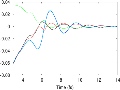
Figure 4: Time evolution of the gradient of each TDPES at position $\langle R(t)\rangle$. Green line: $\frac{\partial}{\partial R}\epsilon^{\rm QS(1)}(\langle R(t)\rangle)$; Red line: $\frac{\partial}{\partial R}\epsilon^{\rm QS(2)}(\langle R(t)\rangle)$; Blue line: $\frac{\partial}{\partial R}\epsilon_{gi}(\langle R(t)\rangle)$; Light blue line: $\frac{\partial}{\partial R}\epsilon^{\rm QS}_{ave}(\langle R(t)\rangle)$; Black line: $\frac{\partial}{\partial R}\epsilon(\langle R(t)\rangle)$.

The black line, which is the gradient of the exact TDPES $\frac{\partial}{\partial R}\epsilon(\langle R(t)\rangle)$, gives the exact force on the nuclei. First we immediately notice that the gradient of the weighted average of the two QSPES $\frac{\partial}{\partial R}\epsilon^{\rm QS}_{ave}(\langle R(t)\rangle)$ (light blue line) (equivalently, the GI component (blue line)) is completely different from the exact force. A semi-classical simulation on the weighted average of the two QSPES would not give the correct nuclear dynamics. We observe instead that, as the localization sets in, the exact force $\frac{\partial}{\partial R}\epsilon(\langle R(t)\rangle)$ coincides with the gradient of one or the other QSPES (red or green). This supports the idea of semiclassical surface-hopping between QSPES Thachuk et al. (1996, 1998); Kelkensberg et al. (2011) at least after the localization begins to set in (time $\sim$6 fs): the exact force on the nuclei is given by the gradient of the exact TDPES, and, when evaluated at the mean nuclear position, coincides with the force from one QSPES or the other, making transitions between them at their avoided crossings. This explains why the semiclassical simulations of Ref. Kelkensberg et al. (2011) had a reasonable agreement with the exact results. Furthermore the figure shows the important role of the gauge-dependent part $\epsilon_{gd}(R,t)$; without this term, the force on the nuclei would be more oscillatory and quite different (blue line in the figure). We note that if instead we choose the gauge where $\epsilon_{gd}(R,t)=0$ then the vector potential $A(R,t)$ will be responsible for the role of effectively reducing the oscillatory structure in the GI term. As stated above, when we choose the gauge where $\epsilon_{gd}(R,t)=0$, then the vector potential $A(R,t)$ plays the role of it according to their relationship: $\tilde{A}(R,t)=\int^{t}_{0}dt^{\prime}\left(-\partial_{R}\epsilon_{gd}(R,t^{\prime})\right)$ Agostini et al. (2015).

III.3 Multiple trajectory Ehrenfest dynamics

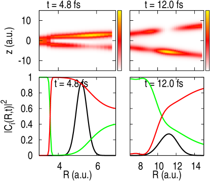
Figure 5: Upper panel: Conditional electron density $|\Phi_{R}(z,t)|^{2}$ obtained from the exact calculation at the indicated times. Lower panel: Squared expansion coefficients of the Born-Oppenheimer expansion $|C_{g}(R,t)|^{2}$ (green) and $|C_{u}(R,t)|^{2}$ (red) of the exact conditional electronic wave function $\Phi_{R}(z,t)$ ($\Phi_{R}(z,t)=C_{g}(R,t)\Phi^{g}_{R}(z)+C_{u}(R,t)\Phi^{u}_{R}(z)$) at the indicated times. The exact nuclear density is also plotted (black).

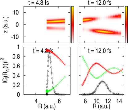
Figure 6: Upper panel: Electron density $|\Phi(z,t|R_{cl}(t))|^{2}$ obtained from multiple trajectory Ehrenfest dynamics calculation at the indicated times (plotted for all trajectories $R_{cl}(t))$). Lower panel: Squared expansion coefficients of the Born-Oppenheimer expansion $|C_{g}(R_{cl}(t))|^{2}$ (green) and $|C_{u}(R_{cl}(t))|^{2}$ (red) of the electronic wave function $\Phi(z,t|R_{cl}(t))$ obtained from multiple trajectory Ehrenfest dynamics calculation ($\Phi(z,t|R_{cl}(t))=C_{g}(R_{cl}(t))\Phi^{g}_{R}(z)+C_{u}(R_{cl}(t))\Phi^{u}_{R}(z)$) at the indiacted times. Nuclear density reconstructed from the distribution of classical trajectories are also plotted (black circle line).

Given that there are several avoided crossings during the localization dynamics, one might ask how well a mean-field surface to propagate the electrons would work. To this end, we run a multiple-trajectory Ehrenfest calculation , and compare the electron and nuclear densities with the exact ones.

In the upper panel of Fig. 5, we plot the conditional electron density $|\Phi_{R}(z,t)|^{2}$ obtained from the exact calculation at indicated times. In the lower panel, we plot its squared expansion coefficients of the Born-Oppenheimer expansion $|C_{g}(R,t)|^{2}$ (green) and $|C_{u}(R,t)|^{2}$ (red) ($\Phi_{R}(z,t)=C_{g}(R,t)\Phi^{g}_{R}(z)+C_{u}(R,t)\Phi^{u}_{R}(z)$), along with the nuclear density (black). In Fig. 6, we plotted electron density $|\Phi(z,t|R_{cl}(t))|^{2}$ obtained from the multiple trajectory Ehrenfest dynamics calculation at the indicated times (plotted for all $800$ trajectories $R_{cl}(t))$. The lower panel shows the squared expansion coefficients of the Born-Oppenheimer expansion $|C_{g}(R_{cl}(t))|^{2}$ (green) and $|C_{u}(R_{cl}(t))|^{2}$ (red) of the electronic wave function $\Phi(z,t|R_{cl}(t))$ obtained from multiple trajectory Ehrenfest dynamics calculation ($\Phi(z,t|R_{cl}(t))=C_{g}(R_{cl}(t))\Phi^{g}_{R}(z)+C_{u}(R_{cl}(t))\Phi^{u}_{R}(z)$). We also show the nucler densities reconstructed from the distribution of classical trajectories obtained from multiple trajectory Ehrenfest dynamics calculation (black circle line).

Comparing the top panels of these figures shows that Ehrenfest dynamics gets the overall structure of the electronic conditional probability reasonably well, however not exactly; in fact, these differences lead to an incorrect prediction of the localization asymmetry. For example, at $t=12.0$ fs at the internuclear separation where the nuclear density is peaked, the projections shown in the lower panels, onto the BO surfaces predicted by Ehrenfest are each close to 0.5, while the exact are closer to 0.6 and 0.4. Given the nature of the BO $g$ and $u$ states in terms of the left and right basis (Sec. II.1), this suggests the localization asymmetry predicted by Ehrenfest is close to 1:0 while the exact is close to 0.8:0.2. Indeed this is verified by the calculation of the asymmetry. Further, throughout the width of the nuclear wavepacket, the Ehrenfest projections remain close to 0.5, while the exact projections fall away, indicating there is a larger degree of decoherence in the exact dynamics, missed in the Ehrenfest dynamics. The differences in the conditional wavefunction and the BO projections is even greater where the nuclear density is small ($R=8\sim 10$ and $R=12\sim 14$).

In the field-free problem of non-adiabatic charge-transfer Abedi et al. (2013); Agostini et al. (2013, 2015); Min et al. , multiple-trajectory Ehrenfest dynamics failed, and this might have been expected given that the density spatially separates (branches) onto two different BO surfaces. In the present case, the nuclear density does not split in space, and actually predicts the nuclear dynamics quite well, but the errors in the electronic dynamics are more significant. Further, it is the same potential that evolves the electrons in the Ehrenfest calculation as in surface-hopping calculations, and this same potential was shown to lack significant structures that the exact potential acting on the electron subsystem (e-TDPES) in Ref. Suzuki et al. (2014) has.

IV Conclusions and Outlook

The TDPES and vector potential arising from the exact factorization of the molecular wavefunction exactly accounts for the coupling to the electronic subsystem as well as coupling to external fields and so it is important to understand their structure, and to relate this to the QSPES which is traditionally used, in order to be able to develop accurate practical mixed quantum-classical methods for strong-field dynamics. In this paper, we have studied the topical phenomenon of laser-induced electron localization in the dissociation of H${}_{2}^{+}$, choosing a gauge where the TDPES is only potential acting on the nuclear system. We found that the gauge-independent component of the TDPES has a mean-field-like character very close to the density-weighted average of the QSPESs and yields an oscillatory force on the nuclei. The gauge-dependent component of the TDPES smoothens the oscillations of the gauge-independent component and together they lead to the correct force.

We demonstrated that running an ensemble of classical nuclear trajectories on this exact TDPES accurately reproduces the exact nuclear dynamics. We found that the force obtained by considering surface-hopping transitions between QSPESs at the laser-induced avoided crossing approximates this exact force, after the localization begins to set in. We showed that errors in multiple-trajectory Ehrenfest dynamics are less significant for the nuclear dynamics than for the electronic dynamics explored in Ref. Suzuki et al. (2014), where it was shown that Ehrenfest yields an incorrect electron localization asymmetry. It is worth noting that the potential acting on the electrons in Ehrenfest dynamics and in surface-hopping schemes lack important step and peak features that the exact potential acting on the electronic system (the e-TDPES) has. Therefore the results of this study show that to reproduce the laser-induced electron localization dynamics accurately by means of a mixed quantum-classical dynamics scheme, we have to go beyond the traditional methods such as surface-hopping or Ehrenfest methods. Our results here encourage the development of mixed quantum-classical schemes based on Eqs (17) and (18) Min et al. to simulate strong-field processes.

Acknowledgments: Partial support from the Deutsche Forschungsgemeinschaft (SFB 762), the European Commission (FP7-NMP-CRONOS), and the U.S. Department of Energy, Office of Basic Energy Sciences, Division of Chemical Sciences, Geosciences and Biosciences under award DE-SC0008623 (NTM),is gratefully acknowledged.

References

- Krausz and Ivanov (2009) F. Krausz and M. Ivanov, Rev. Mod. Phys. 81, 163 (2009).
- Vrakking (2014) M. J. J. Vrakking, Phys. Chem. Chem. Phys. 16, 2775 (2014).
- Lépine et al. (2014) F. Lépine, M. Y. Ivanov, and M. J. J. Vrakking, Nature Photon. 8, 195 (2014).
- Haessler et al. (2010) S. Haessler et al., Nature Phys. 6, 200 (2010).
- Corkum and Krausz (2007) P. B. Corkum and F. Krausz, Nature Phys. 3, 381 (2007).
- Calegari et al. (2014) F. Calegari et al., Science 346, 336 (2014).
- Sansone et al. (2010) G. Sansone et al., Nature 465, 763 (2010).
- He et al. (2007) F. He, C. Ruiz, and A. Becker, Phys. Rev. Lett. 99, 083002 (2007).
- Ray et al. (2009) D. Ray et al., Phys. Rev. Lett. 103, 223201 (2009).
- Singh et al. (2010) K. P. Singh et al., Phys. Rev. Lett. 104, 023001 (2010).
- Fischer et al. (2010) B. Fischer et al., Phys. Rev. Lett. 105, 223001 (2010).
- Calvert et al. (2010) C. R. Calvert et al., J. Phys. B: At. Mol. Opt. Phys. 43, 011001 (2010).
- Kelkensberg et al. (2011) F. Kelkensberg, G. Sansone, M. Y. Ivanov, and M. Vrakking, Phys. Chem. Chem. Phys. 13, 8647 (2011).
- He (2012) F. He, Phys. Rev. A 86, 063415 (2012).
- Liu et al. (2012) K. Liu, Q. Zhang, and P. Lu, Phys. Rev. A 86, 033410 (2012).
- Jia et al. (2014) Z. Jia, Z. Zeng, R. Li, Z. Xu, and Y. Deng, Phys. Rev. A 89, 023419 (2014).
- Wang et al. (2015) Z. Wang, K. Liu, P. Lan, and P. Lu, Phys. Rev. A 91, 043419 (2015).
- Kling et al. (2006) M. F. Kling et al., Science 312, 246 (2006).
- Kremer et al. (2009) M. Kremer et al., Phys. Rev. Lett. 103, 213003 (2009).
- Roudnev et al. (2004) V. Roudnev, B. D. Esry, and I. Ben-Itzahk, Phys. Rev. Lett. 93, 163601 (2004).
- Tong and Lin (2007) X. M. Tong and C. D. Lin, Phys. Rev. Lett. 98, 123002 (2007).
- Graefe and Ivanov (2007) S. Graefe and M. Y. Ivanov, Phys. Rev. Lett. 99, 163603 (2007).
- Rathje et al. (2013) T. Rathje et al., Phys. Rev. Lett. 111, 093002 (2013).
- Kling et al. (2013) N. G. Kling et al., Phys. Rev. Lett. 111, 163004 (2013).
- Li et al. (2014) H. Li et al., J. Phys. B: At. Mol. Opt. Phys. 47, 124020 (2014).
- Lan et al. (2012) P. Lan, E. J. Takahashi, and K. Midorikawa, Phys. Rev. A 86, 013418 (2012).
- Kübel et al. (2014) M. Kübel et al., New J. Phys. 16, 065017 (2014).
- Li et al. (2015) H. Li et al., Phys. Rev. Lett. 114, 123004 (2015).
- Mitrić et al. (2009) R. Mitrić, J. Peterson, and V. Bonac̆ić-Koutecký, Phys. Rev. A 79, 053416 (2009).
- Tavernelli et al. (2010) I. Tavernelli, B. F. E. Curchod, and U. Rothlisberger, Phys. Rev. A 81, 052508 (2010).
- Richer et al. (2011) M. Richer, P. Marquetand, J. González-Vázquez, I. Sola, and L. González, J. Chem. Theory Comput. 7, 1253 (2011).
- Bajo et al. (2012) J. J. Bajo, J. González-Vázquez, I. Sola, J. Santamaria, M. Richer, P. Marquetand, , and L. González, J. Phys. Chem. A 116, 2800 (2012).
- Tully (1990) J. C. Tully, J. Chem. Phys. 93, 1061 (1990).
- Hammes-Schiffer and Tully (1994) S. Hammes-Schiffer and J. C. Tully, J. Chem. Phys. 101, 4657 (1994).
- Tully (1998) J. C. Tully, Faraday Discuss. 110, 407 (1998).
- Dietrich et al. (1996) P. Dietrich, M. Y. Ivanov, F. A. Ilkov, and P. B. Corkum, Phys. Rev. Lett. 77, 4150 (1996).
- Thachuk et al. (1996) M. Thachuk, M. Y. Ivanov, and D. M. Wardlaw, J. Chem. Phys. 109, 4094 (1996).
- Thachuk et al. (1998) M. Thachuk, M. Y. Ivanov, and D. M. Wardlaw, J. Chem. Phys. 109, 5747 (1998).
- Shenvi et al. (2011) N. Shenvi, J. E. Subotnik, and W. Yang, J. Chem. Phys. 134, 144102 (2011).
- Jasper et al. (2006) A. W. Jasper, S. Nangia, C. Zhu, and D. G. Truhlar, Acc. Chem. Res. 39, 101 (2006).
- Bittner and Rossky (1995) E. R. Bittner and P. J. Rossky, J. Chem. Phys. 103, 8130 (1995).
- Akimov et al. (2014) A. V. Akimov, R. long, and O. V. Prezhdo, J. Chem. Phys. 140, 194107 (2014).
- Curchod and Tavernelli (2013) B. F. E. Curchod and I. Tavernelli, J. Chem. Phys. 138, 184112 (2013).
- Makri (2014) N. Makri, Chem. Phys. Lett. 593, 93 (2014).
- Grunwald et al. (2008) R. Grunwald, H. Kim, and R. Kapral, J. Chem. Phys. 128, 164110 (2008).
- Granucci and Persico (2007) G. Granucci and M. Persico, J. Chem. Phys. 126, 134114 (2007).
- Abedi et al. (2010) A. Abedi, N. T. Maitra, and E. K. U. Gross, Phys. Rev. Lett. 105, 123002 (2010).
- Abedi et al. (2012) A. Abedi, N. T. Maitra, and E. K. U. Gross, J. Chem. Phys. 137, 22A530 (2012).
- Abedi et al. (2013) A. Abedi, F. Agostini, Y. Suzuki, and E. K. U. Gross, Phys. Rev. Lett. 110, 263001 (2013).
- Agostini et al. (2013) F. Agostini, A. Abedi, Y. Suzuki, and E. K. U. Gross, Mol. Phys. 111, 3625 (2013).
- Agostini et al. (2015) F. Agostini, A. Abedi, Y. Suzuki, S. K. Min, N. T. Maita, and E. K. U. Gross, J. Chem. Phys. 142, 084303 (2015).
- Shin and Metiu (1995) S. Shin and H. Metiu, J. Chem. Phys. 102, 23 (1995).
- Suzuki et al. (2014) Y. Suzuki, A. Abedi, N. T. Maitra, K. Yamashita, and E. K. U. Gross, Phys. Rev. A 89, 040501(R) (2014).
- Dietrich and Corkum (1992) P. Dietrich and P. B. Corkum, J. Chem. Phys. 97, 3187 (1992).
- Zuo and Bandrauk (1995) T. Zuo and A. Bandrauk, Phys. Rev. A 52, R2511 (1995).
- Seideman et al. (1995) T. Seideman, M. Y. Ivanov, and P. B. Corkum, Phys. Rev. Lett. 75, 2819 (1995).
- Kawata et al. (1998) I. Kawata, H. Kono, and Y. Fujimura, Chem. Phys. Lett. 289, 546 (1998).
- Kawata et al. (1999) I. Kawata, H. Kono, and Y. Fujimura, J. Chem. Phys. 110, 11152 (1999).
- Kono et al. (2004) H. Kono et al., Chem. Phys. 304, 203 (2004).
- Kato et al. (2009) T. Kato, H. Kono, M. Kanno, Y. Fujimura, and K. Yamanouchi, Laser Phys. 19, 1712 (2009).
-
Note (1)
A set of 800 trajectories is propagated according to
and(36)
where the initial conditions are sampled from the phase-space distribution corresponding to .(37) - (62) S. K. Min, F. Agostini, and E. K. U. Gross, arXiv:1504.0025 [physics.chem-ph] .