Unambiguous atomic Bell measurement assisted by multiphoton states

Abstract

We propose and theoretically investigate an unambiguous Bell measurement of atomic qubits assisted by multiphoton states. The atoms interact resonantly with the electromagnetic field inside two spatially separated optical cavities in a Ramsey-type interaction sequence. The qubit states are postselected by measuring the photonic states inside the resonators. We show that if one is able to project the photonic field onto two coherent states on opposite sites of phase space, an unambiguous Bell measurement can be implemented. Thus our proposal may provide a core element for future components of quantum information technology such as a quantum repeater based on coherent multiphoton states, atomic qubits and matter-field interaction.

1 Introduction

Establishing well-controlled entanglement between spatially separated quantum systems is essential for quantum communication Briegel98 ; Duer99 . At its core a quantum repeater employs entanglement which is generated and distributed among intermediary nodes positioned not too distant from each other. Entanglement purification Bennett ; Deutsch enables the distillation of a high-fidelity state from a large number of low-fidelity entangled pairs and with the help of entanglement swapping procedures Zuk the two end points of a repeater are entangled. There are many different implementation proposals for quantum repeaters, utilizing completely different systems and entanglement distribution protocols Sangouard . A promising approach towards these schemes is to require some compatibility with existing optical communication networks. The proposal of van Loock et al. vanLoock1 ; vanLoock2 ; vanLoock3 ; vanLoock4 is such an approach where the repeater scheme employs coherent multiphoton states. These proposals assume dispersive interaction between the atomic qubits and the single-mode of the radiation field. This imposes limitations on the photonic postselection. It was shown that these limitations can be overcome in the case of resonant atom-field interactions Bernad1 ; Bernad2 and it was demonstrated for one building block of a repeater, namely the entanglement generation between spatially separated and neighbouring nodes. A natural extension of this approach is to propose resonant atom-field interaction based schemes also for the other building blocks. In the case of entanglement swapping a complete atomic Bell measurement is required.

Bell measurements play a central role also in entanglement-assisted quantum teleportation Bennett93 and in superdense coding Bennett92 . In the case of photonic qubits theoretical proposals Knill ; Pittman ; Munro have been made and experimental realizations have already been carried out Kim ; Schuck . However, for atomic qubits there are still experimental difficulties which restrain implementations of complete Bell measurements where projections onto the four Bell states can be accomplished. There exist experimental proposals that rely on the application of a controlled NOT gate Pellizzari ; Lloyd . These proposals have the drawback that experimental implementations of two-qubit gates have still complications to attain high fidelity Schmidt-Kaler ; Isenhower ; Noelleke . This implies that the fidelity of the generated Bell states is also affected Isenhower . A proposal focusing specifically on a non-invasive atomic Bell measurement with high fidelity is still missing.

In previous work we have introduced a protocol to project onto one Bell state with high fidelity Torres2014 based on atomic qubits which interact sequentially with coherent field states prepared in two cavities. The field states emerging after the interactions are postselected by balanced homodyne photodetection. In this paper we expand our previous work to accomplish the projection onto all four Bell states provided the protocol is successful. Thus we introduce an unambiguous Bell measurement of two atomic qubits with the help of coherent multiphoton field states. We demonstrate that the possibility of implementing field projections onto two coherent states on opposite sites of phase space implies the possibility to realize an unambiguous Bell measurement. Our protocol has a finite probability of error depending on the initial states of the atoms. This is due to the imperfect overlap of the field contributions with coherent states. Nevertheless, it is an unambiguous protocol as there are four successful events that lead to postselection of four different Bell states. The scheme is based on basic properties of the two-atom Tavis-Cummings model Tavis and on resonant matter-field interactions which are already under experimental investigation Casabone1 ; Casabone2 ; Reimann ; Nussmann2005 . These considerations make our scheme compatible with a quantum repeater or a quantum relay based on coherent multiphoton states, atomic qubits and resonant matter-field interaction. Our proposal demonstrates that scenarios involving the two-atom Tavis-Cummings model are rich enough to enable future Bell measurement implementations.

The paper is organized as follows. In Sec. 2 we introduce the theoretical model and analyse the solutions of the field state with the aid of the Wigner function in phase space. Furthermore, we provide approximate solutions of the global time dependent state vector that facilitate the analysis of the system. In Sec. 3 we present a scheme to perform an unambiguous Bell measurement provided one is able to project a single mode photonic field onto coherent states. In Sec. 4 we provide a numerical analysis of the fidelity of the projected Bell states and discuss general features of the protocol. Details of our calculations are presented in Appendices A and B.

2 Theoretical model

2.1 Basic equations

In this section we recapitulate basic features of the two-atom Tavis-Cummings model Tavis . This model has been considered previously to study the dynamics of entanglement Torres2014 ; Jarvis ; Rodrigues ; Kim2002 ; Tessier . The model describes the interaction between two atoms $A$ and $B$ and a single mode of the radiation field with frequency $\omega$. The two identical atoms have ground states $|{0}\rangle_{i}$ and excited states $|{1}\rangle_{i}$ ($i\in\{A,B\}$) separated by an energy difference of $\hbar\omega$. In the dipole and rotating-wave approximation the Hamiltonian in the interaction picture is given by

$$\hat{H} =\hbar g\sum_{i=A,B}\left(\hat{\sigma}^{+}_{i}\hat{a}+\hat{\sigma}^{-}_{i}\hat{a}^{\dagger}\right)$$ (1)

where $\hat{\sigma}^{+}_{i}=|{1}\rangle\langle{0}|_{i}$ and $\hat{\sigma}^{-}_{i}=|{0}\rangle\langle{1}|_{i}$ are the atomic raising and lowering operators ($i\in\{A,B\}$), and $\hat{a}$ ($\hat{a}^{\dagger}$) is the annihilation (creation) operator of the single mode field. The coupling between the atoms and the field is characterized by the vacuum Rabi frequency $2g$.

The time evolution of the system can be evaluated for an initial pure state as

$$|{\Psi_{t}}\rangle=e^{-i\hat{H}t/\hbar}|{\Psi_{0}}\rangle.$$ (2)

We are interested in the case where the atoms and the cavity are assumed to be prepared in the product state

$$|{\Psi_{0}}\rangle=\Big{(}c^{-}|{\Psi^{-}}\rangle+c^{+}|{\Psi^{+}}\rangle+d_{\phi}^{-}|{\Phi^{-}_{\phi}}\rangle+d_{\phi}^{+}|{\Phi^{+}_{\phi}}\rangle\Big{)}|{\alpha}\rangle,$$ (3)

with the radiation field considered initially in a coherent state Glauber ; Perelomov

$$|{\alpha}\rangle=\sum_{n=0}^{\infty}e^{-\frac{|\alpha|^{2}}{2}}\frac{\alpha^{n}}{\sqrt{n!}}|{n}\rangle,\quad\alpha=\sqrt{\overline{n}}\,e^{i\phi},$$ (4)

with mean photon number $\bar{n}$ and photon-number states $|{n}\rangle$. The parameters $c^{\pm}$ and $d_{\phi}^{\pm}$ are the initial probability amplitudes of the orthonormal Bell states

$$|{\Psi^{\pm}}\rangle =\tfrac{1}{\sqrt{2}}\left(|{0,1}\rangle\pm|{1,0}\rangle\right),$$

$$|{\Phi^{\pm}_{\phi}}\rangle =\tfrac{1}{\sqrt{2}}\left(e^{-i\phi}|{0,0}\rangle\pm e^{i\phi}|{1,1}\rangle\right),$$ (5)

with the atomic states $|{i,j}\rangle=|{i}\rangle_{A}|{j}\rangle_{B}$ ($i,j\in\{0,1\}$). We have chosen an atomic orthonormal basis containing the states $|{\Psi^{\pm}}\rangle$ as the state $|{\Psi^{-}}\rangle|{n}\rangle$ is an invariant state of the system. This is explained in Appendix A where we present the full solution of the temporal state vector. The other two Bell states $|{\Phi_{\phi}^{\pm}}\rangle$ depend on the initial phase $e^{i\phi}$ of the coherent state. They appear naturally in the Tavis-Cummings model due to the exchange of excitations between atoms and cavity, and are involved in an approximate solution of the state vector that facilitate the analysis of the dynamics. Before showing the detailed form of our solution, let us give an overview of the dynamical features that impose relevant time scales in the system.

2.2 Collapse and revival phenomena

The collapse and revival phenomena of the Jaynes-Cummings model and of the two-atom Tavis-Cummings model play an essential role in the quantum information protocols presented in Refs. Bernad1 ; Torres2014 ; Jarvis . This behaviour was first found in the time dependent atomic population in the Jaynes-Cummings model Eberly1980 when the field is initially prepared in a coherent state: The populations display Rabi oscillations that cease after a collapse time $t_{c}$ and appear again at a revival time $t_{r}$. In the case of the two atom Tavis-Cummings model, the collapse and revival time of the Rabi oscillations are given by

$$t_{r}=\frac{\pi}{g}\sqrt{4\bar{n}+2},\quad t_{c}=\frac{1}{\sqrt{2}g}.$$ (6)

These time scales have been previously introduced and can be found, for instance, in Refs. Jarvis ; Eberly1980 . As they play an essential role in the dynamics of the system it is convenient to introduce the rescaled time

$$\tau=t/t_{r}=tg/\pi\sqrt{4\bar{n}+2}.$$ (7)

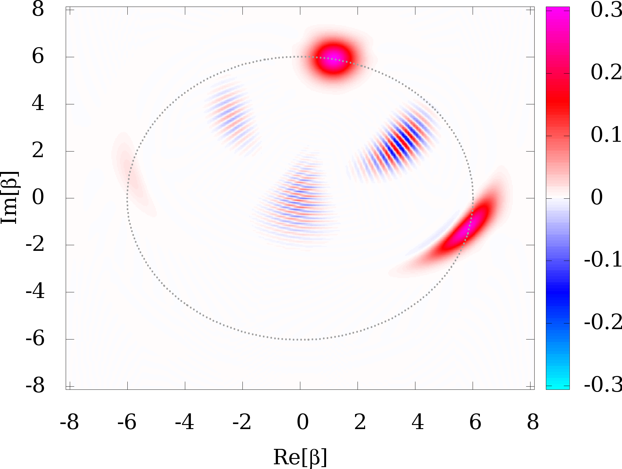
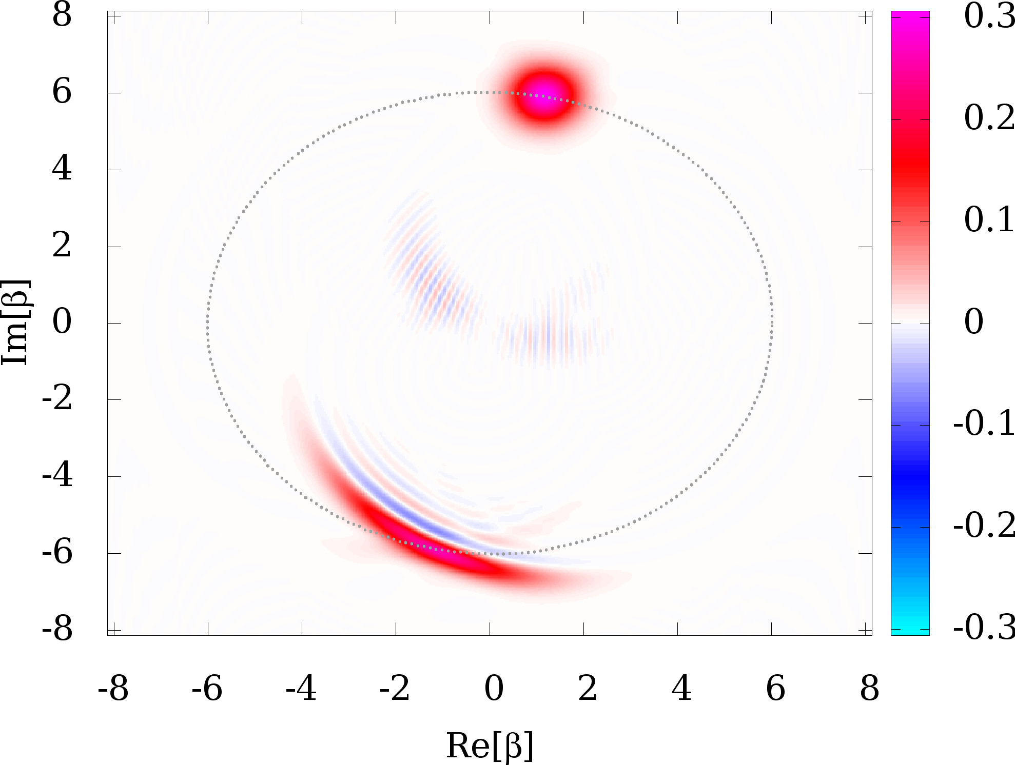
Figure 1: Wigner function of the cavity field after the interaction with two two-level atoms at times $\tau=1/4$ (top) and $\tau=1/2$ (bottom) with the rescaled time of Eq. (7). The initial states of the atoms are defined by the parameters: $c^{-}=0.5554$, $c^{+}=0.3213+i0.5004$, $d^{-}_{\phi}=-0.2053+i0.3726$, $d^{+}_{\phi}=0.1046+i0.3819$, and the parameter $\alpha=\sqrt{36.16}e^{i1.37}$ characterizes the initial coherent sate.

Let us explain these phenomena by visualizing the phase space of the radiation field with the aid of the Wigner function Schleich ; Risken

$$W_{t}(\beta,\beta^{*})=\frac{1}{\pi^{2}}\int{\rm Tr}\left\{\hat{\varrho}_{t}\,e^{\zeta\hat{a}^{\dagger}-\zeta^{*}\hat{a}}\right\}e^{\beta\zeta^{*}-\beta^{*}\zeta}d^{2}\zeta,$$ (8)

with the complex numbers $\beta$ and $\zeta$. The operator $\hat{\varrho}_{t}={\rm Tr}_{\rm atoms}\left\{|{\Psi_{t}}\rangle\langle{\Psi_{t}}|\right\}$ is the density matrix of the field state obtained after taking partial trace over the atomic degrees of freedom from the full density matrix corresponding to the state vector in Eq. (2). In Fig. 1 we show the Wigner function after interaction times $\tau=1/4$ in the top panel and $\tau=1/2$ in the bottom panel. The circular shape corresponds to the initial coherent state $|{\alpha}\rangle$. This contribution to the field remains stationary as long as there is an initial contribution of the state $|{\Psi^{-}}\rangle$. The reason is that $|{\Psi^{-}}\rangle|{n}\rangle$ is an invariant state of the system. There are two other contributions to the field that rotate around the origin. In the top panel of Fig. 1 it can be noticed that for an interaction time of $\tau/4$ they have completed a quarter of cycle. At the bottom, the situation at interaction time $\tau/2$ is shown where half a rotation has been completed. The interference fringes between the field contributions signify that there are coherent superposition between these states of the field. The behaviour of the field state in phase space explain the phenomena: Rabi oscillations cease (collapse) when the field contributions are well separated, e.g. at time $\tau/4$, and revive when the field contributions overlap, e.g. at $\tau/2$ or the main revival at $\tau$ when all the field constituents coincide at the position of the initial coherent state.

2.3 Approximation of the state vector

The full solution to the time dependent state vector of the two atoms Tavis-Cummings model has already been presented in previous work, see for instance Kim2002 ; Torres2010 . Coherent state approximations have also been considered in the past Torres2014 ; Jarvis ; Rodrigues ; Gea-Banacloche . In this context, the eigenfrequencies of the Hamiltonian (1) that depend on the photonic number $n$ are expanded in a first order Taylor series around the mean photon number $\bar{n}$. However, the coherent state description is accurate only for times well below the revival time. In this work we go beyond the coherent state approximation by considering second order contributions of the eigenfrequencies around $\bar{n}$. The details can be found in the Appendix A where it is shown that the time dependent state vector of the system can be approximated by

$$|{\Psi^{\rm A}_{\tau}}\rangle= \frac{1}{N_{\tau}}\left(c^{-}|{\Psi^{-}}\rangle+d_{\phi}^{-}|{\Phi^{-}_{\phi}}\rangle\right)|{\alpha}\rangle+$$

$$\frac{c^{+}-d^{+}_{\phi}}{2N_{\tau}}\left(|{\Psi^{+}}\rangle-|{\Phi^{+}_{\phi+2\pi\tau}}\rangle\right)|{\alpha_{\tau}^{+}}\rangle+$$

$$\frac{c^{+}+d^{+}_{\phi}}{2N_{\tau}}\left(|{\Psi^{+}}\rangle+|{\Phi^{+}_{\phi-2\pi\tau}}\rangle\right)|{\alpha_{\tau}^{-}}\rangle,$$ (9)

with the photonic states

$$|{\alpha_{\tau}^{\pm}}\rangle=\sum_{n=0}^{\infty}\frac{\alpha^{n}e^{-\frac{|\alpha|^{2}}{2}}}{\sqrt{n!}}e^{\pm i2\pi\tau\left[\bar{n}+1+n-\frac{(n-\bar{n})^{2}}{4\bar{n}+2}\right]}|{n}\rangle$$ (10)

and with the normalization factor

$$N_{\tau}=\Big{(}1 +{\rm Re}[(c^{+}+d^{+}_{\phi})^{\ast}(c^{+}-d^{+}_{\phi})\langle{\alpha^{-}_{\tau}}|{\alpha^{+}_{\tau}}\rangle]\sin^{2}(2\pi\tau)$$

$$+2{\rm Re}[d^{-}_{\phi}(d^{+}_{\phi})^{\ast}]{\rm Im}[\langle{\alpha^{-}_{\tau}}|{\alpha}\rangle]\sin(2\pi\tau).$$

$$+2{\rm Im}[(c^{+})^{\ast}d^{-}_{\phi}]{\rm Re}[\langle{\alpha^{-}_{\tau}}|{\alpha}\rangle]\sin(2\pi\tau)\Big{)}^{1/2}.$$ (11)

The quantity $\langle{\alpha^{-}_{\tau}}|{\alpha}\rangle$ is evaluated in Appendix B and an approximate expression is given in Eq. (29).

In order to test the validity of Eq. (9) we have considered the fidelity $F(\tau)=|\langle{\Psi^{\rm A}_{\tau}}|{\Psi_{t_{r}\tau}}\rangle|^{2}$ of the approximated state vector with respect to the exact result given in Eq. (20). In Fig. 2 we have plotted the results of numerical evaluations of the fidelity $F(\tau)$ for different values of the mean photon number $\bar{n}$. It can be noticed that the validity of this approximation improves with increasing mean photon number $\bar{n}$. In the Appendix A it is discussed that our approximation is valid provided the condition $\tau\ll\sqrt{\bar{n}}/2\pi$ is fulfilled.

The form of the solution given in Eq. (9) allows a simple analysis of the dynamics. It is written in terms of an orthonormal atomic basis of Bell states and is therefore suitable for the analysis of the atomic entanglement. In particular, it is interesting to note that for an initial state without a contribution of the state $|{\Phi^{-}_{\phi}}\rangle$, i.e. $d_{\phi}^{-}=0$, a photonic projection that discriminates the state $|{\alpha}\rangle$ from the states $|{\alpha_{\tau}^{\pm}}\rangle$ can postselect the atomic Bell state $|{\Psi^{-}}\rangle$. In Ref. Torres2014 we studied this Bell state projection and found that its implementation requires a flexible restriction for the interaction time: it has to be below the revival time and above the collapse time given in Eq. (6). In the following we concentrate in a more specific interaction time. We analyze the dynamics at the specific interaction time $\tau=1/2$. This analysis will allow us to introduce in Sec. 3 a protocol to perform the four Bell state projections.

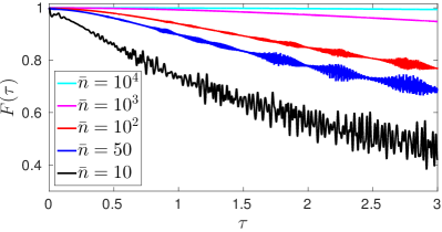
Figure 2: Fidelity of the total state of Eq. (9) with respect to the exact solution given by Eq. (20) as a function of the time $\tau$ in Eq. (7) scaled in terms of the revival time $t_{r}$: Five curves are presented for different values of the mean photon number $\bar{n}$ as described in the legend. The rest of the parameters are the same as in Fig. 1.

2.4 Basic dynamical features at scaled interaction time $\tau=1/2$

There are two main reasons for studying in detail the case with scaled interaction time $\tau=1/2$. The first one is that the time dependent atomic states in Eq. (9) coincide, i.e.

$$|{\Phi_{\phi+\pi}^{\pm}}\rangle=|{\Phi_{\phi-\pi}^{\pm}}\rangle=-|{\Phi_{\phi}^{\pm}}\rangle.$$ (12)

The second reason is that the photonic states $|{\alpha_{1/2}^{\pm}}\rangle$ have completed half a rotation in phase space and lie on the opposite site to the initial coherent state $|{\alpha}\rangle$ whereby overlapping with the coherent state $|{-\alpha}\rangle$. This means that at this interaction time and for $|\alpha|\gg 1$, the initial photonic state $|{\alpha}\rangle$ can be approximately distinguished from the other two states $|{\alpha_{1/2}^{\pm}}\rangle$. However, the states $|{\alpha_{1/2}^{\pm}}\rangle$ overlap significantly. This can be noticed in Fig. 1 where we have plotted the Wigner function. The circular shape corresponds to the initial coherent state $|{\alpha}\rangle$, while the distorted ellipses on the opposite site of the phase space correspond to the states $|{\alpha^{\pm}_{1/2}}\rangle$. To distinguish these two components of the field it is convenient to conceive an experiment that is able to project the field state onto the coherent states $|{\pm\alpha}\rangle$.

In order to study the projection onto the state $|{\pm\alpha}\rangle$, one has to evaluate its overlap with the photonic states of the state vector in Eq. (9). First we consider the overlaps that can be neglected for large value $\bar{n}$, namely

$$\langle{\alpha}|{-\alpha}\rangle=e^{-2\bar{n}},\quad\langle{\alpha}|{\alpha_{1/2}^{\pm}}\rangle\propto e^{-\frac{2\pi^{2}}{4+\pi^{2}}\bar{n}}.$$ (13)

The explicit form of the overlap $\langle{\alpha}|{\alpha_{1/2}^{\pm}}\rangle$ is given in Eq. (28) of the Appendix B where its approximation is also evaluated. The nonvanishing overlaps in the limit of large mean photon number are $\langle{\alpha}|{\alpha}\rangle=1$ and

$$\langle{-\alpha}|{\alpha_{1/2}^{\pm}}\rangle \approx\sqrt{\frac{2}{\sqrt{4+\pi^{2}}}}e^{\mp i\left(\frac{1}{2}\arctan\frac{\pi}{2}-(\bar{n}+1)\pi\right)}.$$ (14)

The expression in Eq. (14) is also evaluated in detail in Appendix B. This overlap is real valued if the mean photon number $\bar{n}=|\alpha|^{2}$ fulfills the relation

$$\bar{n}=m+\tfrac{1}{2\pi}\arctan\tfrac{\pi}{2},\quad{\rm with}\quad m\in\mathbb{N}.$$ (15)

If the condition in Eq. (15) is fulfilled and if we suppose an initial atomic state with no contribution from the state $|{\Phi^{+}_{\phi}}\rangle$, i.e. $d^{+}_{\phi}=0$, then it can be verified that a projection onto the field state $|{-\alpha}\rangle$ postselects the atoms in the unnormalized atomic Bell state $\sqrt{b}c^{+}|{\Psi^{+}}\rangle$, with

$$b=2/\sqrt{4+\pi^{2}}.$$ (16)

The success probability of this projection is given by $b|c^{+}|^{2}$ which is proportional to the initial probability of this particular Bell state $|{\Psi^{+}}\rangle$. The factor $b$ is the result of our inability to project perfectly and simultaneously onto both field states $|{\alpha^{\pm}_{1/2}}\rangle$. In the next section we present a protocol that can perform postselection of the four Bell states regardless of the initial state of the atoms.

3 An unambiguous Bell measurement

In this section we introduce a protocol which implements a projection onto four orthogonal atomic Bell states of Eq. (5) for any given initial condition of the atoms. The scheme we propose requires interactions between the atoms with two different cavities as sketched in Fig. 3. The interaction time between the atoms and the electromagnetic field in each cavity is assumed to be $\tau=1/2$. The field in the first (second) cavity has to be prepared in a coherent state $|{\alpha}\rangle$ ($|{i\alpha}\rangle$). After the interaction with the first cavity the resulting field is projected onto the initial state $|{\alpha}\rangle$. In case of failure a projection onto the state $|{-\alpha}\rangle$ is performed. The projection of the field postselects the atoms in a state that has contribution of only two of the Bell states. This postselected atomic state is taken as initial condition to interact with a second cavity prepared in the state $|{i\alpha}\rangle$. The atoms are assumed to evolve freely for a time $\tau_{f}$ before interacting with a second cavity. This does not affect the protocol as the free Hamiltonian commutes with the interaction Hamiltonian in Eq. (1). After the interaction of the atoms with the second cavity, the field in the second cavity is projected onto $|{i\alpha}\rangle$ and if this fails another projection onto the state $|{-i\alpha}\rangle$ is performed. With this field state projection, the atoms are finally postselected in a unit fidelity Bell state. In what follows we discuss in detail all the possible outcomes of the protocol. There is a finite probability to fail completely when none of the coherent state field projections is successful. This is discussed in Sec. 4.

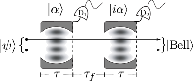
Figure 3: Schematic representation of the proposed atomic Bell measurement: Two atomic qubits interact with the electromagnetic field inside two independent cavities in a Ramsey-type interaction sequence. Different projections on the field states inside the cavities, recorded by detectors ${\rm D}_{1}$ and ${\rm D}_{2}$, result in a postselection of atomic Bell states as described in Table 1.

3.1 Projection onto $|{\alpha}\rangle$ in the first cavity

Let us consider a successful projection onto the field state $|{\alpha}\rangle$ of the first cavity. In this case the atoms are postselected in the state

$$\frac{1}{\sqrt{P_{1}}}\left(c^{-}|{\Psi^{-}}\rangle+d_{\phi+\pi/2}^{+}|{\Phi^{+}_{\phi+\pi/2}}\rangle\right)$$ (17)

with probability $P_{1}=|c^{-}|^{2}+|d_{\phi}^{-}|^{2}$. To write this state we have also considered the relations

$$|{\Phi_{\phi+\pi/2}^{\pm}}\rangle=-i|{\Phi^{\mp}_{\phi}}\rangle,\quad d^{\pm}_{\phi+\pi/2}=id^{\mp}_{\phi}.$$ (18)

The postselected atomic state of Eq. (17) is taken as initial condition for the interaction with the second cavity prepared in the coherent state $|{i\alpha}\rangle$ as depicted in Fig. 3. Two scenarios are possible for the projection of the field in the second cavity. In the first place we consider a projection onto the coherent state $|{i\alpha}\rangle$ where the atoms are postselected in the state $|{\Psi^{-}}\rangle$ with probability $P_{11}=|c^{-}|^{2}/P_{1}$. This can be verified from Eq. (9) as the new initial state does not have a contribution of $|{\Phi^{-}_{\phi+\pi/2}}\rangle$. As the projections performed in the first and second cavity are independent events the state $|{\Psi^{-}}\rangle$ can be projected with overall success probability $P_{1}P_{11}=|c^{-}|^{2}$, the initial probability weight of this state before the protocol. The second possibility is to project onto the state $|{-i\alpha}\rangle$. In that case the atoms are postselected in the state $|{\Phi_{\phi}^{-}}\rangle=i|{\Phi_{\phi+3\pi/2}^{+}}\rangle$ provided the condition in Eq. (15) is fulfilled. This can be verified using Eq. (9) with an initial coherent state $|{i\alpha}\rangle$ and the atoms initially in the state of Eq. (17) that has no contribution of $|{\Psi^{+}}\rangle$. The success probability for this event is $P_{10}=b|d_{\phi}^{-}|^{2}/P_{1}$. Correspondingly the projection onto the atomic state $|{\Phi^{-}_{\phi}}\rangle$ occurs with overall success probability $P_{1}P_{10}=b|d_{\phi}^{-}|^{2}$. This is proportional to its initial probability weight but not equal. The proportionality factor $b$ is given in Eq. (16) and accounts to the imperfect projection onto the states $|{i\alpha_{1/2}^{\pm}}\rangle$.

Field state in detector ${\rm D}_{1}$	Field state in detector ${\rm D}_{2}$	Atomic state $|{{\rm Bell}}\rangle$	Probability
$|{\alpha}\rangle$	$|{i\alpha}\rangle$	$|{\Psi^{-}}\rangle$	$|c^{-}|^{2}$
$|{\alpha}\rangle$	$|{-i\alpha}\rangle$	$|{\Phi^{-}_{\phi}}\rangle$	$b|d^{-}_{\phi}|^{2}$
$|{-\alpha}\rangle$	$|{i\alpha}\rangle$	$|{\Phi^{+}_{\phi}}\rangle$	$b|d^{+}_{\phi}|^{2}$
$|{-\alpha}\rangle$	$|{-i\alpha}\rangle$	$|{\Psi^{+}}\rangle$	$b^{2}|c^{+}|^{2}$

Table 1: Summary of the Bell state protocol assisted by photonic state measurements. The first (second) column indicates the photonic field that has to be selected in the first (second) cavity by detector ${\rm D}_{1}$ (${\rm D}_{2}$) in the interaction sequence depicted in Fig. 3. The third column indicates the resulting atomic state with the probability of occurrence given in the last column with $b=2/\sqrt{4+\pi^{2}}\approx 0.537$. The protocol fails with probability $(1-b)(|d^{-}_{\phi}|^{2}+|d^{+}_{\phi}|^{2})+(1-b^{2})|c^{+}|^{2}$.

3.2 Projection onto $|{-\alpha}\rangle$ in the first cavity

Now we consider a successful projection onto the coherent state $|{-\alpha}\rangle$ in the first cavity. In this situation the atoms are postselected in the state

$$\sqrt{\frac{b}{P_{0}}}\left(c^{+}|{\Psi^{+}}\rangle-d^{-}_{\phi+\pi/2}|{\Phi^{-}_{\phi+\pi/2}}\rangle\right)$$ (19)

with probability $P_{0}=b|c^{+}|^{2}+b|d_{\phi}^{+}|^{2}$. We have used the relations in Eqs. (12) and (18).

The normalized state of Eq. (19) is taken as initial condition to interact with the second cavity prepared in the coherent state $|{i\alpha}\rangle$. There are two scenarios in the projection of the second cavity. First we consider a successful projection onto the state $|{i\alpha}\rangle$. As the initial state of Eq. (19) does not have any contribution of $|{\Psi^{-}}\rangle$, the atoms are postselected in the state $|{\Phi^{+}_{\phi}}\rangle=i|{\Phi^{-}_{\phi+3\pi/2}}\rangle$. This occurs with success probability $P_{01}=b|d^{+}_{\phi}|^{2}/P_{0}$. Thus the state $|{\Phi^{+}_{\phi}}\rangle$ is postselected with an overall success probability $P_{0}P_{01}=b|d^{+}_{\phi}|^{2}$. A second possible situation is a projection onto the state $|{-i\alpha}\rangle$ in the second cavity. In this situation the atoms are postselected in the state $|{\Psi^{+}}\rangle$. This can be noted from Eq. (9) as the second initial atomic state of Eq. (19) does not have any contribution of the state $|{\Phi^{+}_{\phi+\pi/2}}\rangle$. The success probability of this event is $P_{00}=|c_{+}|^{2}b^{2}/P_{0}$. It implies an overall success probability of postselecting state $|{\Psi^{+}}\rangle$ of $P_{0}P_{00}=b^{2}|c^{+}|^{2}$.

4 Discussion of the protocol

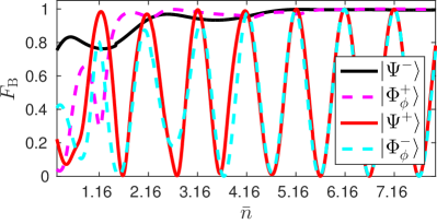
Figure 4: Fidelity $F_{\rm B}$ of the projected atomic Bell states as a function of the initial mean photon number of the fields inside the cavities: The interaction time in both cavities is given by $\tau=1/2$, i.e. half the revival time (see Eq. (7)) and the rest of the initial conditions are the same as in Fig. 2. Each curve correspond to a different Bell state as explained in the legend.

4.1 Fidelity of the postselected Bell states

In order to test our protocol based on the approximations of Eqs. (9) and (14) we have numerically evaluated the fidelity $F_{\rm B}=|\langle{\rm Bell}|{\psi}\rangle|^{2}$ of the resulting Bell states in each of the four possible successful outcomes. The state $|{\rm Bell}\rangle$ stands for any of the four Bell states of Eq. (5). The state $|{\psi}\rangle$ is the exact numerical solution after the protocol and depends either on the $\bar{n}$ or $\tau$. In Fig. 4 we have plotted the fidelity $F_{\rm B}$ for the different Bell states as a function of the mean photon number $\bar{n}=|\alpha|^{2}$ of the initial coherent field states $|{\alpha}\rangle$ and $|{i\alpha}\rangle$. Interestingly, the protocol already shows high fidelity (above 0.9) even for small mean photon numbers. The results improve for increasing values of $\bar{n}$ in accordance to the validity of our approximation for high photon number explained in Sec. 2. The fidelity has an oscillatory periodic behaviour and maxima are achieved close to the values of $\bar{n}$ predicted by Eq. (15), i.e. when $\bar{n}$ is an integer number plus the constant $\arctan(\pi/2)/2\pi\approx 0.16$. A possible error $\delta\bar{n}$ in the previous value has to fulfill the condition $\delta\bar{n}\ll 1/\pi$ to ensure a high fidelity of the atomic states. It should be mentioned that in the extreme opposite case in which both cavities are initially prepared in the vacuum state, i.e. $\bar{n}=0$, the proposed protocol does not work. According to Eq. (9) the four orthogonal Bell states are paired up with three field states and in order to filter out all Bell states they have to be orthogonal. This requirement can only be fulfilled in the limit of high mean number of photons.

To test the sensitivity of the protocol with respect to the interaction time we have also evaluated the fidelity $F_{\rm B}$ as a function of the scaled interaction time $\tau$ between the atoms and the cavities. The results with the initial atomic conditions of Fig. 2 are plotted in Fig. 5. We present the results for an initial coherent state with mean photon number $\bar{n}=36+\arctan(\pi/2)/2\pi$. The black solid curve represents the fidelity of projecting onto state $|{\Psi^{-}}\rangle$ and it shows a constant unit fidelity in the time interval of the plot. The stability of this result has also been discussed in Ref. Torres2014 and is due to the fact that $|{\Psi^{-}}\rangle$ is a special invariant atomic state of the two-atom Tavis-Cummings model. The fidelity of the state $|{\Phi^{+}_{\phi}}\rangle$ also shows robustness with respect to the interaction time $\tau$. This is due to the fact that this state is obtained after projecting onto $|{i\alpha}\rangle$ which is the stationary initial state of the second cavity. Advantages of the two-atom Tavis-Cummings model for generating this particular Bell state have also been mentioned previously in Ref. Rodrigues . The other two fidelities of projections onto states $|{\Phi^{-}_{\phi}}\rangle$ and $|{\Psi^{+}}\rangle$ oscillate as a function of $\tau$. In this case the second field projection is performed onto field state $|{-i\alpha}\rangle$ and this in turn has to “catch” the time dependent states $|{i\alpha_{\tau}^{\pm}}\rangle$. Therefore, the oscillations are originated by the overlap between photonic states $\langle{-\alpha}|{\alpha^{\pm}_{\tau}}\rangle$ that is calculated in the Appendix B. One can estimate that the fidelity $F_{\rm B}$ around $\tau=1/2$ oscillates with frequency $2(\bar{n}+1)$. The optimal interaction time according to Eq. (29) is $\tau=1/2$ where the absolute value of the overlap attains its maximum. A possible error $\varepsilon$ in the scaled interaction time $\tau=1/2+\varepsilon$ has to be restricted to the condition $|\varepsilon|\ll 1/4\pi(\bar{n}+1)$.

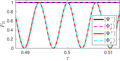
Figure 5: Fidelity $F_{\rm B}$ of the projected atomic Bell states as a function of the scaled interaction time $\tau$ (see Eq. (7)) on both cavities: The initial conditions are the same as in Fig. 1 with $\bar{n}=36.16$. Each curve correspond to a different Bell state of Eq. 5 as explained in the legend.

4.2 Experimental constraints

Our protocol requires that the pair of atoms interact with two different coherent states. This could be realized, for instance, by transporting and positioning the atomic qubits in separate cavities. Current experimental realizations report coherent transport and controlled positioning of neutral atoms in optical cavities Reimann ; Nussmann2005 ; Khudaverdyan ; Brakhane , where a dipole trap is used as a conveyor belt to displace them. Two trapped ions have also been reported to be coupled in a controlled way to an optical resonator Casabone1 ; Casabone2 . The cavity can be shifted with respect to ions, allowing to tune the coupling strength between ions and optical cavity. In this setting, instead of transporting the atoms to a different cavity, the same cavity might be shifted to a position where it decouples from the atoms until the measurement is achieved. Then it would have to be prepared and shifted again for a second interaction with the ions.

In our discussion we have not considered losses. The effects of decoherence can be neglected in the strong coupling regime, where the coupling strength $g$ between atoms and cavity is much larger than the spontaneous decay rate of the atoms $\gamma$ and the photon decay rate of the cavity $\kappa$. Actually, in our setting due to the specific interaction time $t_{r}/2\approx\pi\sqrt{\bar{n}}/g$ tighter constraints are required. More specifically, for the cavities we require $1/\kappa\gg\pi\sqrt{\bar{n}}/g$ and for the atoms $1/\gamma\gg\pi\sqrt{\bar{n}}/g$. The experiment by Khudaverdyan et al. Khudaverdyan achieved ratios $g/\kappa=32.5$ and $g/\gamma=5$ which imply that $\bar{n}\ll 2.5$. For a single atom interacting with a cavity, the experiment by Birnbaum et al. Birnbaum involves ratios $g/\kappa=8.26$, $g/\gamma=13.03$ and if there is a possibility to attain these parameters for a two-atom scenario then the constraint would yield $\bar{n}\ll 7$. In microwave cavities Raimond , the numbers are $g/\kappa\approx 60$ and $g/\gamma\approx 3000$ which lead to the condition $\bar{n}\ll 360$. Thus, the coherence requirement of our proposal is in the reach of current experimental capabilities.

We have mentioned that our protocol requires the implementation of projections onto coherent states. We are not aware of an experimental solution to this problem. However, coherent states and the vacuum state are routinely distinguished in current experiments, see e.g. Wittmann . A successful measurement of the vacuum state is achieved when no photons are detected. Therefore, for our purposes it would be sufficient to displace the state of the field in such a way that the field contributions $|{\alpha_{1/2}^{\pm}}\rangle$ are close to the vacuum state. This can be achieved by driving the optical cavity with a resonant laser. The Hamiltonian describing this situation in the interaction picture is $\hat{V}=\hbar(\Omega^{\ast}\hat{a}+\Omega\hat{a}^{\dagger})$. Under this interaction the states of the field evolve under the influence of the evolution operator $\hat{U}_{t_{d}}=\exp{(-it_{d}\hat{V}/\hbar)}$ that can be identified with the displacement operator $\hat{D}(\alpha)=\exp{(\alpha\hat{a}^{\dagger}-\alpha^{\ast}\hat{a})}$ provided the interaction strength of the laser $\Omega$ and the driving time $t_{d}$ are adjusted as $\Omega t_{d}=i\alpha$. In this way one is able perform the displacement $\hat{D}(\alpha)|{-\alpha}\rangle=|{0}\rangle$. Finally, we conceive a photodetection of the field with three possible outputs; $1)$ No signal, meaning a projection onto the vacuum state, i.e. $|{-\alpha}\rangle$ in the undisplaced picture; $2)$ a weak signal indicating a failure of the protocol; 3) a strong signal would come from the field state $|{2\alpha}\rangle$.

4.3 Probabilities in the protocol

A summary of all the possible outcomes of the protocol is given in the Table 1. We note that summing the probabilities of all the successful outcomes of the protocol results in an overall success probability of $P_{\rm T}=b+(1-b)(|c^{-}|^{2}-b|c^{+}|^{2})$ which depends on the initial state of the system. The complementary probability $1-P_{\rm T}$ corresponds to events that lead to failure of the protocol. There is a possible failure after a successful projection onto $|{\alpha}\rangle$ but unsuccessful projection onto $|{-i\alpha}\rangle$. This occurs with probability $(1-b)|d_{\phi}^{-}|^{2}$. It also might happen that the projection onto the field state $|{-\alpha}\rangle$ in the first cavity is unsuccessful. This takes place with probability $(1-b)(|c^{+}|^{2}+|d_{\phi}^{+}|^{2})$. Finally, it is possible that both projections in the first and second cavity fail with probability $(1-b)b|c^{+}|^{2}$. Summing all these failure probabilities leads to $1-P_{\rm T}=(1-b)(|d^{-}_{\phi}|^{2}+|d_{\phi}^{+}|^{2})+(1-b^{2})|c^{+}|^{2}$.

5 Conclusion

We have presented a proposal of an unambiguous Bell measurement on two atomic qubits with almost unit-fidelity. The theoretical description of the scheme involves the resonant two-atom Tavis-Cummings model and a Ramsey-type sequential interaction of both atoms with single modes of the electromagnetic field in two spatially separated cavities. The first and second cavities are initially prepared in coherent states $|{\alpha}\rangle$ and $|{i\alpha}\rangle$ respectively. The interaction time can be adjusted by controlling the velocities of the two atoms passing trough the cavities. Our discussion has concentrated on basic properties of the two-atom Tavis-Cummings model in the limit of high photon numbers. We have derived an approximate solution of the dynamical equation which is expressed as a sum of three terms correlating atomic and field states. A superposition of two atomic Bell states is correlated with the initial coherent state. Superpositions of the other two Bell states are correlated with two time dependent field states. In phase space these time dependent contributions of the field state overlap on the opposite site to the initial coherent state $|{\alpha}\rangle$ ($|{i\alpha}\rangle$) in the first (second) cavity at an interaction time of half the revival time. For this reason we have proposed projections onto the two coherent states $|{\alpha}\rangle$ and $|{-\alpha}\rangle$ in the first cavity, and $|{i\alpha}\rangle$ and $|{-i\alpha}\rangle$ in the second cavity. In order to obtain almost unit fidelity atomic Bell states the mean photon number has to be restricted to the condition given in Eq. (15). Our protocol has a finite error probability due to the imperfect projection onto the time dependent contributions of the field states in the cavities that overlap with $|{-\alpha}\rangle$ and $|{-i\alpha}\rangle$. Nevertheless, the four successful events of our protocol summarized in Table 1 unambiguously project onto four different Bell states with almost unit fidelity.

In view of current experimental realizations of quantum information protocols in the field of cavity quantum electrodynamics the scheme discussed in this work requires cutting edge technology. An experimental implementation would require accurate control of the interaction time and of the average number of photons in the cavity. Furthermore, the coherent evolution of the joint system must be preserved. This imposes the condition that the characteristic time of photon damping in the cavity and of atomic decay have to be much larger than the interaction time that scales with the square root of the mean photon number in the cavity. Finally, we point out that the implementation of a von Neumann coherent state projection is, up to our knowledge, an open problem that has to be considered in future investigations. If these obstacles are overcome, our proposal offers a key component for quantum information technology such as a multiphoton based hybrid quantum repeater.

Appendix A Approximations with large mean photon numbers

In this Appendix we present the derivation of the time dependent state vector of Eq. (9). It has been shown in Ref. Torres2014 ; Torres2010 that the time evolution of any initial state in the form of Eq. (3) can be obtained from the solution of the eigenvalue problem of the two-atom Tavis-Cummings Hamiltonian (1). The exact solution can be written in the following form

$$|{\Psi_{t}}\rangle=|{0,0}\rangle|{\chi_{t}^{0}}\rangle+|{1,1}\rangle|{\chi^{1}_{t}}\rangle+|{\Psi^{+}}\rangle|{\chi^{+}_{t}}\rangle+c_{-}|{\Psi^{-}}\rangle|{\alpha}\rangle$$ (20)

with the relevant photonic states

$$|{\chi^{0}_{t}}\rangle =c_{0}\,p_{0}|{0}\rangle+\sum_{n=1}^{\infty}\tfrac{\sqrt{n}\left(\xi_{n,t}^{-}-\xi_{n,t}^{+}\right)+\sqrt{n-1}\xi_{n}}{\sqrt{2n-1}}|{n}\rangle,$$

$$|{\chi^{1}_{t}}\rangle =\sum_{n=2}^{\infty}\tfrac{\sqrt{n-1}\left(\xi_{n,t}^{-}-\xi_{n,t}^{+}\right)-\sqrt{n}\xi_{n}}{\sqrt{2n-1}}|{n-2}\rangle,$$

$$|{\chi^{+}_{t}}\rangle =\sum_{n=1}^{\infty}\left(\xi_{n,t}^{-}+\xi_{n,t}^{+}\right)|{n-1}\rangle,$$ (21)

and with the aid of the following abbreviations

$$\xi_{n,t}^{\pm}=\frac{e^{\pm i\omega_{n}t}}{2}\left(c_{+}p_{n-1}\mp\tfrac{\sqrt{n}\,c_{0}p_{n}+\sqrt{n-1}\,c_{1}p_{n-2}}{\sqrt{2n-1}}\right),$$

$$\xi_{n}=\frac{\sqrt{n-1}\,c_{0}p_{n}-\sqrt{n}\,c_{1}p_{n-2}}{\sqrt{2n-1}},\quad\omega_{n}=g\sqrt{4n-2}.$$

The coefficients $p_{n}$ are initial probability amplitudes of the photon number states $|{n}\rangle$ of the initial field state $|{\alpha}\rangle$. The coefficients $c_{0}$ and $c_{1}$ are the initial probability amplitudes of the states $|{0,0}\rangle$ and $|{1,1}\rangle$ and are related to the probability amplitudes of the state in Eq. (3) by

$$d_{\phi}^{\pm} =\frac{c_{0}e^{i\phi}\pm c_{1}e^{-i\phi}}{\sqrt{2}}.$$ (22)

The expressions of Eq. (21) can be significantly simplified approximately by taking into account that the field is initially prepared in a coherent state $|{\alpha}\rangle$ with photonic distribution $p_{n}=\exp(-\bar{n}/2+i\phi)\sqrt{\bar{n}^{n}/n!}$ and by assuming a large mean photon number $\bar{n}=|\alpha|^{2}\gg 1$. In such case the photonic distribution has the following property

$$p_{n}=\sqrt{\frac{\bar{n}}{n}}e^{i\phi}p_{n-1}\approx e^{i\phi}p_{n-1}.$$ (23)

Applying this approximation to the states of Eq. (21) we find the following approximations

$$|{\chi^{0}_{t}}\rangle\approx\sum_{n=1}^{\infty}\tfrac{(c_{+}+d_{\phi}^{+})e^{-i\omega_{n}t}-(c_{+}-d_{\phi}^{+})e^{i\omega_{n}t}+2d_{\phi}^{-}}{2\sqrt{2}}p_{n-1}|{n}\rangle,$$

$$|{\chi^{1}_{t}}\rangle\approx\sum_{n=2}^{\infty}\tfrac{(c_{+}+d_{\phi}^{+})e^{-i\omega_{n}t}-(c_{+}-d_{\phi}^{+})e^{i\omega_{n}t}-2d_{\phi}^{-}}{2\sqrt{2}}p_{n-1}|{n-2}\rangle,$$

$$|{\chi^{+}_{t}}\rangle\approx\sum_{n=1}^{\infty}\tfrac{(c_{+}+d_{\phi}^{+})e^{-i\omega_{n}t}+(c_{+}-d_{\phi}^{+})e^{i\omega_{n}t}}{2}p_{n-1}|{n-1}\rangle.$$

In order to simplify these expressions we perform a Taylor expansion in the frequencies $\omega_{n}$ around $\bar{n}+1$ as

$$\omega_{n}/g \approx\sqrt{4\bar{n}+2}+2\frac{n-\bar{n}-1}{\sqrt{4\bar{n}+2}}-2\frac{(n-\bar{n}-1)^{2}}{(4\bar{n}+2)^{3/2}}.$$ (24)

The previous second order expansion is valid provided the third order contribution multiplied by $gt$ is negligible. This imposes the restriction on the interaction time

$$t\ll\frac{(4\bar{n}+2)^{5/2}}{4g\bar{n}^{3/2}}\approx\bar{n}/g.$$ (25)

For the rescaled time $\tau=gt/\pi\sqrt{4\bar{n}+2}$ used in the main text this implies $\tau\ll\sqrt{\bar{n}}/2\pi$. In this approximation the field states can be written as

$$|{\chi^{0}_{t}}\rangle \approx e^{-i\phi}\tfrac{(c_{+}+d_{\phi}^{+})|{\alpha_{t}^{-},-1}\rangle-(c_{+}-d_{\phi}^{+})|{\alpha_{t}^{+},-1}\rangle+2d_{\phi}^{-}|{\alpha}\rangle}{2\sqrt{2}},$$

$$|{\chi^{1}_{t}}\rangle \approx e^{i\phi}\tfrac{(c_{+}+d_{\phi}^{+})|{\alpha_{t}^{-},1}\rangle-(c_{+}-d_{\phi}^{+})|{\alpha_{t}^{+},1}\rangle-2d_{\phi}^{-}|{\alpha}\rangle}{2\sqrt{2}},$$

$$|{\chi^{+}_{t}}\rangle \approx\tfrac{(c_{+}+d_{\phi}^{+})|{\alpha^{-}_{t},0}\rangle+(c_{+}-d_{\phi}^{+})|{\alpha^{+}_{t},0}\rangle}{2},$$ (26)

with

$$|{\alpha_{t}^{\pm},j}\rangle =\sum_{n=0}^{\infty}e^{-\frac{|\alpha|^{2}}{2}}\frac{\alpha^{n}}{\sqrt{n!}}e^{\pm i\left(\nu+2\tfrac{n-\bar{n}+j}{\nu}-2\frac{(n-\bar{n}+j)^{2}}{\nu^{3}}\right)gt}|{n}\rangle$$

$$\approx e^{\pm ij2\pi\tau}|{\alpha^{\pm}_{\tau}}\rangle,$$ (27)

$j\in\{-1,0,1\}$ and $\nu=\sqrt{4\bar{n}+2}$. Furthermore, the states $|{\alpha_{\tau}^{\pm}}\rangle$ are defined by Eq. (10). We neglected the contribution of $j$ in the quadratic term of the exponent in Eq. (27). This can be justified given the fact a Poisson distribution with high mean value is almost symmetrically centered around its mean with variance equal to its mean. This implies that the maximal relevant value in the quadratic term is given by

$${\rm max}\left\{\frac{(n-\bar{n}+j)^{2}}{\nu}\right\}\approx 2+\frac{2j}{\sqrt{\bar{n}}}+\frac{j}{2\bar{n}},$$

which shows that the contribution of $j=-1,0,1$ to this term is negligible for $\bar{n}\gg 1$.

Finally, using the approximations of Eq. (26) and (27) in Eq. (20) and separating the atomic states accompanying to the photonic states $|{\alpha_{\tau}^{\pm}}\rangle$ and $|{\alpha}\rangle$ yields the result of Eq. (9).

Appendix B Evaluation of $\langle{\alpha}|{\alpha^{\pm}_{\tau}}\rangle$ and $\langle{-\alpha}|{\alpha^{\pm}_{\tau}}\rangle$

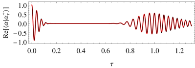
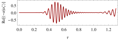
Figure 6: Top (bottom) figure: Real part of the overlap $\langle{\alpha}|{\alpha^{+}_{\tau}}\rangle$ ($\langle{-\alpha}|{\alpha^{+}_{\tau}}\rangle$) as function of the rescaled time $\tau$. The red curve was evaluated using the exact expression in the first line of Eq. (28) and the black narrow line corresponds to the approximation given in Eq. (29). The mean photon number is $\bar{n}=12.16$.

In this appendix we investigate the overlaps between the field states $|{\alpha^{\pm}_{\tau}}\rangle$ and $|{\pm\alpha}\rangle$ defined in Eqs. (10) and (4) respectively. Using the index $j\in\{-1,1\}$ one can write a single expression for the four overlaps as

$$\langle{j\alpha}|{\alpha_{\tau}^{\pm}}\rangle=\sum_{n=0}^{\infty}\frac{\bar{n}^{n}j^{n}}{n!e^{\bar{n}}}e^{\pm i2\pi\tau\left[\bar{n}+1+n-\frac{(n-\bar{n})^{2}}{4\bar{n}+2}\right]}$$ (28)

$$\approx\frac{e^{\pm i(\bar{n}+1)2\pi\tau}}{\sqrt{2\pi\bar{n}}}\sum_{n=-\infty}^{\infty}e^{\pm i\pi n\left(2\tau+\frac{1-j}{2}\right)-\frac{(1\pm i\pi\tau)}{2\bar{n}}(n-\bar{n})^{2}}$$

$$=\frac{e^{\pm i(\bar{n}+1)2\pi\tau}}{\sqrt{1\pm i\pi\tau}}\sum_{n=-\infty}^{\infty}e^{\pm i2\pi\bar{n}\left(\tau+\frac{1-j}{4}\pm n\right)-\frac{2\pi^{2}\bar{n}}{1\pm i\pi\tau}\left(\tau+\frac{j-1}{4}\pm n\right)^{2}}.$$

In the second line we have approximated the Poisson distribution by a normal distribution and we have extended the sum to $-\infty$. These approximations are valid in the limit $\bar{n}\gg 1$. In the third line we have used the Poisson summation formula Bellman which in the case of a Gaussian sum can be expressed as

$$\sum_{n=-\infty}^{\infty}e^{i2\pi un-s(n-\bar{n})^{2}}=\sqrt{\frac{\pi}{s}}\sum_{n=-\infty}^{\infty}e^{i2\pi\bar{n}(n+u)-\frac{\pi^{2}}{s}(n+u)^{2}},$$

with ${\rm Re}[s]>0$. The last expression in Eq. (28) involves a summation of Gaussian terms with variance $(1+\pi^{2}\tau^{2})/4\pi^{2}\bar{n}$. This variance is very small provided the condition $4\bar{n}\gg\tau^{2}$ is fulfilled. If this requirement is met, there exists a dominant contribution in the summation that corresponds to the value of $n$ where $|\tau+(1-j)/4\pm n|$ achieves its minimum value. This minimum can be evaluated as

$$f_{j}(\tau)={\rm frac}\left(\tau+\tfrac{1-j}{4}+\tfrac{1}{2}\right)-\tfrac{1}{2},$$

where ${\rm frac}(x)$ denotes the fractional part of $x$. By considering only the dominant term of the last summation in Eq. (28) one can find the following approximation of the overlap between field states

$$\langle{j\alpha}|{\alpha^{\pm}_{\tau}}\rangle \approx\frac{e^{\pm i2\pi[\bar{n}f_{j}(\tau)+(\bar{n}+1)\tau]}}{\sqrt{1\pm i\pi\tau}}e^{-\frac{2\pi^{2}\bar{n}}{1\pm i\pi\tau}[f_{j}(\tau)]^{2}},$$ (29)

with $j\in\{-1,1\}$. This result for $\tau=1/2$ and $j=-1$ has been rewritten in polar form in Eq. (14) of the main text, where we used that $f_{-1}(1/2)=0$. In Eq. (13) we have used that $f_{1}(1/2)=-1/2$. In the top panel of Fig. 6 have plotted the real part of the overlap $\langle{\alpha}|{\alpha^{+}_{\tau}}\rangle$ as a function of the rescaled time $\tau$. The evaluation of the exact expression is shown in red and the approximation in black. The collapse and revival phenomena are well described by the approximation of the overlap in Eq. (29). Similar treatment to describe the collapse and revival phenomena in the Jaynes-Cummings model has been presented in Ref. Karatsuba . In the bottom figure of Fig. 6 we have plotted the real part of the overlap $\langle{-\alpha}|{\alpha^{+}_{\tau}}\rangle$.

References

- (1) H.-J. Briegel, W. Dür, J. I. Cirac and P. Zoller, Phys. Rev. Lett. 81, 5932 (1998).
- (2) W. Dür, H.-J. Briegel, J. I. Cirac and P. Zoller, Phys. Rev. A 59, 169 (1999).
- (3) C. H. Bennett, G. Brassard, S. Popescu, B. Schumacher, J. A. Smolin, and W. K. Wootters, Phys. Rev. Lett. 76, 722 (1996).
- (4) D. Deutsch, A. Ekert, R. Jozsa, C. Macchiavello, S. Popescu, and A. Sanpera, Phys. Rev. Lett. 77, 2818 (1996).
- (5) M. Zukowski, A. Zeilinger, M. A. Horne, and A. K. Ekert, Phys. Rev. Lett. 71, 4287 (1993).
- (6) N. Sangouard, C. Simon, H. de Riedmatten, and N. Gisin, Rev. Mod. Phys. 83, 33 (2011).
- (7) P. van Loock, T. D. Ladd, K. Sanaka, F. Yamaguchi, K. Nemoto, W. J. Munro, and Y. Yamamoto, Phys. Rev. Lett. 96, 240501 (2006).
- (8) T. D. Ladd, P. van Loock, K. Nemoto, W. J. Munro, and Y. Yamamoto, New J. Phys. 8, 184 (2006).
- (9) P. van Loock, N. Lütkenhaus, W. J. Munro, and K. Nemoto, Phys. Rev. A 78, 062319 (2008).
- (10) D. Gonta and P. van Loock, Phys. Rev. A 88, 052308 (2013).
- (11) J. Z. Bernád and G. Alber, Phys. Rev. A 87, 012311 (2013).
- (12) J. Z. Bernád, H. Frydrych, and G. Alber, J. Phys. B 46, 235501 (2013).
- (13) J.M. Torres, J.Z. Bernád and G. Alber, Phys. Rev. A 90, 012304 (2014).
- (14) C. H. Bennett, G. Brassard, C. Crépeau, R. Jozsa, A. Peres, and W. K. Wootters, Phys. Rev. Lett. 70, 1895 (1993).
- (15) C. H. Bennett and S. J. Wiesner, Phys. Rev. Lett. 69, 2881 (1992).
- (16) E. Knill, R. Laflamme and G. Milburn,Nature 409, 46 (2001).
- (17) T. B. Pittman, M. J. Fitch, B. C Jacobs, and J. D. Franson, Phys. Rev. A 68, 032316 (2003).
- (18) W. J. Munro, K. Nemoto, T. P. Spiller, S. D. Barrett, P. Kok, and R. G. Beausoleil, J. Opt. B: Quantum Semiclass. Opt. 7, 135 (2005).
- (19) Y.-H. Kim, S. P. Kulik and Y. Shih, Phys. Rev. Lett. 86, 1370 (2001).
- (20) C. Schuck, G. Huber, C. Kurtseifer, and H. Weinfurter, Phys. Rev. Lett. 96, 190501 (2006).
- (21) T. Pellizzari, S. A. Gardiner, J. I. Cirac and P. Zoller, Phys. Rev. Lett. 21, 3788 (1995).
- (22) S. Lloyd, M. S. Shahriar, J. H. Shapiro and P. R. Hemmer, Phys. Rev. Lett. 87, 167903 (2001).
- (23) F. Schmidt-Kaler, H. Häffner, M. Riebe, S. Gulde, G. P. T. Lancaster, T. Deuschle, C. Becher, C. F. Roos, J. Eschner, and R. Blatt, Nature 422, 408 (2003).
- (24) L. Isenhower, E. Urban, X. L. Zhang, A. T. Gill, T. Henage, T. A. Johnson, T. G. Walker, and M. Saffman, Phys. Rev. Lett. 104, 010503 (2010).
- (25) C. Nölleke, A. Neuzner, A. Reiserer, C. Hahn, G. Rempe, and S. Ritter, Phys. Rev. Lett. 110, 140403 (2013).
- (26) M. Tavis and F. W. Cummings, Phys. Rev. 170, 279 (1968).
- (27) B. Casabone, A. Stute, K. Friebe, B. Brandstätter, K. Schüppert, R. Blatt, and T. E. Northup, Phys. Rev. Lett. 111, 100505, (2013).
- (28) B. Casabone, K. Friebe, B. Brandstätter, K. Schüppert, R. Blatt, and T. E. Northup, Phys. Rev. Lett. 114, 023602 (2015).
- (29) R. Reimann, W. Alt, T. Kampschulte, T. Macha, L. Ratschbacher, N. Thau, S. Yoon, and D. Meschede, Phys. Rev. Lett. 114, 023601 (2015).
- (30) S. Nußmann, M. Hijlkema, B. Weber, F. Rohde, G. Rempe, and A. Kuhn, Phys. Rev. Lett. 95 173602 (2005).
- (31) R. J. Glauber, Phys. Rev. 131, 2766 (1963).
- (32) A. Perelomov, Generalized Coherent States and Their Applications (Springer-Verlag Berlin Heidelberg 1986).
- (33) C. E. A. Jarvis, D. A. Rodrigues, B. L. Györffy, T. P. Spiller, A. J. Short, and J. F. Annett, New J. Phys. 11, 103047 (2009).
- (34) D. A. Rodrigues, C. E. A. Jarvis, B. L. Györffy, T. P. Spiller and J. F. Annett, J. Phys.: Condens. Matter 20 075211 (2008).
- (35) M. S. Kim, J. Lee, D. Ahn, P. L. Knight, Phys. Rev. A, 65 040101(R) (2002).
- (36) T. E. Tessier, I. H. Deutsch, A. Delgado, and I. Fuentes-Guridi Phys. Rev. A, 68 062316 (2003).
- (37) J. H. Eberly, N. B. Narozhny and J. J. Sanchez-Mondragon, Phys. Rev. Lett. 44 1323 (1980).
- (38) W. P. Schleich Quantum Optics in Phase Space (Wiley-VCH, Weinheim, 2001).
- (39) K. Vogel and H. Risken, Phys. Rev. A 40, 2847 (1989).
- (40) J. M. Torres, E. Sadurni, and T. H. Seligman, J. Phys. A 43, 192002 (2010).
- (41) J. Gea-Banacloche, Phys. Rev. A, 44 5913 (1991).
- (42) M. Khudaverdyan, W. Alt, I. Dotsenko, T. Kampschulte, K. Lenhard, A. Rauschenbeutel, S. Reick, K. Schörner, A. Widera and D. Meschede, New J. Phys., 10 073023 (2008).
- (43) S. Brakhane, W. Alt, T. Kampschulte, M. Martinez-Dorantes, R. Reimann, S. Yoon, A. Widera, and D. Meschede Phys. Rev. Lett., 109 173601 (2012).
- (44) J. M. Raimond, M. Brune, and S. Haroche, Rev. Mod. Phys., 73 565 (2001).
- (45) K. M. Birnbaum, A. Boca, R. Miller, A. D. Boozer, T. E. Northup, and H. J. Kimble, Nature 436, 87 (2005).
- (46) C. Wittmann, M. Takeoka, K. N. Cassemiro, M. Sasaki, Gerd. Leuchs, and U. L. Andersen, Phys. Rev. Lett., 101 210501 (2008).
- (47) R.E. Bellman, A Brief introduction to theta functions (Holt, Rinehart and Winston, New York, 1961).
- (48) A. A. Karatsuba, and E. A. Karatsuba, J. Phys. A, 42 195304 (2009).