High-resolution 3D phase imaging using a partitioned detection aperture: a wave-optic analysis

Abstract

Quantitative phase imaging has become a topic of considerable interest in the microscopy community. We have recently described one such technique based on the use of a partitioned detection aperture, which can be operated in a single shot with an extended source [Opt. Lett. 37, 4062 (2012)]. We follow up on this work by providing a rigorous theory of our technique using paraxial wave optics, where we derive fully three-dimensional spread functions for both phase and intensity. Using these functions we discuss methods of phase reconstruction for in- and out-of-focus samples, insensitive to weak attenuations of light. Our approach provides a strategy for detection-limited lateral resolution with an extended depth of field, and is applicable to imaging smooth and rough samples.

1 Introduction

Quantitative phase imaging reveals optical path variations in almost transparent (and also specularly reflecting) objects, and thus provides useful information for biological or industrial applications. Different strategies exist to obtain phase information [1], most of which are interferometric and rely on monochromatic illumination. In the case of quasi-monochromatic illumination, optical phase is not well defined and interferometric techniques only measure changes in optical phase relative to a self-reference provided, for example, by spatial filtering [2, 3, 4], or shearing [5, 6, 7]. Alternatively, gradients in optical phase can be inferred non-interferometrically based purely on intensity imaging, using, for example, the transport of intensity equation [8, 9, 10], or by directly measuring changes in the direction of flux density, or local light tilt [11, 12, 13, 14, 15, 16, 17]. We have recently introduced a method to measure local light tilts that is based on the use of a partitioned detection aperture [18]. By associating local light tilts with phase gradients and integrating these over space, we thus obtain quantitative images of phase. The method is passive, single-shot, provides high spatial resolution, and works with quasi-broadband, partially coherent illumination. A reflection version of the method is described in [19], as is a version implemented for closed-loop adaptive optic wavefront sensing [20].

The purpose of this work is to present an in depth theoretical analysis of our partitioned aperture wavefront imaging technique that goes significantly beyond the cursory and mostly experimental expositions we provided in our previous reports [18, 19]. In particular, our previous reports were based on smooth phase approximations and on strict assumptions regarding the numerical apertures of both the illumination and detection optics of our system, which ultimately limited spatial resolution. In this paper, we generalize to phases that are not necessarily smooth (though they must remain small), and we relax our assumptions regarding numerical apertures, enabling access to improved spatial resolution. Finally, we extend our analysis to three dimensions by considering samples that can be out of focus, and describing a refocusing strategy conceptually similar to that used in light field [21, 22] or integral [23] imaging. The goal of this paper is to provide a rigorous theoretical underpinning to partitioned aperture wavefront imaging, which has been long overdue. In the process, we also discuss strategies to expand on its capabilities.

2 Phase imaging with a partitioned aperture

A schematic of our method is shown in Fig. 1. A phase sample is modeled as a thin transparent layer of variable optical thickness. The sample is trans-illuminated by an axially symmetric beam of light of uniform intensity, which is characterized at each point by a distribution of light rays filling a well-defined square illumination numerical aperture. After traversing the sample, the light is imaged by a device that comprises a lens of focal length $f_{e}$, a partitioned lens assembly of focal length $f_{d}$ and a camera, arranged in a $3f$ imaging configuration. For simplicity, we assume that the lens assembly is masked such that each individual lens in the assembly appears square.

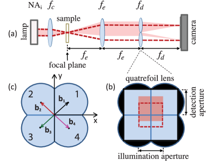
Figure 1: (a) Partitioned detection aperture microscope in transmission mode. (b) Image of the illumination aperture on the face of the partitioned assembly of four lenses: dashed square identifies the aperture in the absence of a phase sample, the shifted solid square demonstrates the effect of light refraction by the sample. (c) Four off-axis lens assembly: the locations of optical axes of the four lenses with respect to the optical axis of the system are identified by vectors ${\bf b}_{i}$, $i=1..4$. A larger aperture (shading) ensures the detection apertures are square.

The purpose of the quatrefoil lens assembly is to simultaneously project multiple separated images onto the camera (here four), each acquired from a different oblique direction. Local tilts of light rays caused by the sample thus lead to local intensity differences in the projected images, as can be understood from Fig. 1. In the absence of a sample, the square illumination aperture forms a centered image on the surface of the lens assembly, and one obtains four images of uniform and equal intensities at the camera. When a phase sample is present, the intensity distribution between the images changes. Indeed, phase slopes at a given sample point cause the light rays through that point to tilt and the image of the illumination aperture from that point to shift (Fig. 1b). Correspondingly, the four images of the sample point projected onto the camera exhibit unequal intensities. If the detection aperture is large enough there is no vignetting of the illumination aperture image and one can uniquely retrieve the tilts from the intensity distribution of the four images. As we discuss below, the retrieved light tilts provide a measure of sample-induced phase gradients, and hence, ultimately, of phase.

2.1 Partitioned aperture imaging

The four off-axis lenses form four images at the detector plane. To begin, we consider light propagating through one of the lenses shifted from the optical axis of the system by vector ${\bf b}$. Throughout this work we confine ourselves to the paraxial wave approximation [24] and assume, for simplicity, unit magnification (i.e. $f_{e}=f_{d}$). The field at the detector (camera) plane is thus given by

$$E_{d}({\bf r},t) = e^{i6\pi kf_{e}}e^{i\pi\frac{k}{f_{e}}{\bf r}^{2}}\int{\rm d^{2}}{\bf r}_{0}e^{-i2\pi\frac{k}{f_{e}}{\bf r}_{0}{\bf b}}$$ (1)

$$\times\,{\rm CSF_{d}}\left({\bf r}-{\bf r}_{0}\right)E_{0}({\bf r}_{0},t),$$

where $\lambda=1/k$ is the wavelength, the coordinate ${\bf r}={\bf r}_{i}-{\bf b}$ accounts for the shift of the image with respect to the position ${\bf b}$ of the detection lens, and $E_{0}({\bf r}_{0},t)$ is the illumination field at time $t$ at the focal plane (in the absence of a sample). The detection numerical aperture of the system is defined by that of an individual off-axis detection lens $f_{d}$, and the coherent spread function of each lens, when centered, is given by

$${\rm CSF_{d}}({\bf r})=\left(\frac{k}{f_{e}}\right)^{2}\int{\rm d^{2}}{\bf r}^{\prime}\,e^{i2\pi\frac{k}{f_{e}}{\bf r}^{\prime}{\bf r}}{\rm A_{d}}({\bf r}^{\prime})$$ (2)

where ${\rm A_{d}}({\bf r})$ is the square aperture function of an individual lens.

The intensity at the detector plane is defined as $I_{d}({\bf r})=\langle E_{d}({\bf r},t)E^{*}_{d}({\bf r},t)\rangle$, where the average $\langle...\rangle$ is taken over a time scale much longer than the coherence time of the light. The intensity is expressed as a weighted sum of the mutual intensity $J_{0}({\bf r}_{0c},{\bf r}_{0d})$ over the focal plane

$$I_{d}({\bf r}) = \int{\rm d^{2}}{\bf r}_{0c}{\rm d^{2}}{\bf r}_{0d}\,e^{-i2\pi\frac{k}{f_{e}}{\bf b}{\bf r}_{0d}}J_{0}({\bf r}_{0c},{\bf r}_{0d})$$ (3)

$$\times\,{\rm CSF_{d}}\left({\bf r}-{\bf r}_{0+}\right){\rm CSF^{*}_{d}}\left({\bf r}-{\bf r}_{0-}\right),$$

where $J_{0}({\bf r}_{0c},{\bf r}_{0d})=\langle E_{0}({\bf r}_{0+},t)E^{*}_{0}({\bf r}_{0-},t)\rangle$ characterizes spatial correlations of the illumination field between pairs of points in the focal plane, and ${\bf r}_{0\pm}={\bf r}_{0c}\pm{\bf r}_{0d}/2$. The off-axis shift of the detection lens is accounted for by the phase factor with the spatial frequency proportional to the oblique detection tilt angle ${\bf b}/f_{e}$. Eq. (3) serves as the basis for what follows.

2.2 Partially coherent illumination

In our optical system a transparent sample is trans-illuminated by a uniform beam of quasi-monochromatic light resulting from Köhler illumination with a condenser lens of focal length $f_{c}$. The spatial extent of the light source is defined by the aperture function ${\rm A_{c}}({\bf r})$. We consider a spatially incoherent source described by the function $J_{c}({\bf r}_{c},{\bf r}_{d})=k^{-2}I_{0}\,{\rm A_{c}}({\bf r}_{c})\delta({\bf r}_{d})$, where $I_{0}$ is the uniform intensity of the source, and $\delta({\bf r})$ is the two-dimensional Dirac delta function. The illumination mutual intensity at the focal plane (in the absence of a sample) is then given by $J_{0}({\bf r}_{c},{\bf r}_{d})=I_{0}\mu_{0}({\bf r}_{d})$, where the illumination coherence function is given by

$$\mu_{0}({\bf r})=\frac{1}{f_{c}^{2}\Omega_{c}}\int{\rm d^{2}}{\bf r}^{\prime}e^{-i2\pi\frac{k}{f_{c}}{\bf r}^{\prime}{\bf r}}{\rm A_{c}}({\bf r}^{\prime}),$$ (4)

and we defined the solid angle $\Omega_{c}=\int{\rm d^{2}}{\bf r}\left|{\rm A_{c}}({\bf r}^{\prime})\right|^{2}/f_{c}^{2}$ of the source as viewed through the condenser lens. As noted above, we assume a square illumination aperture of size $2d_{c}\times 2d_{c}$. The illumination coherence function is thus separable $\mu_{0}({\bf r})={\rm sinc}\left(\pi x/a_{i}\right){\rm sinc}\left(\pi y/a_{i}\right)$, where $a_{i}=\lambda/(2{\rm NA_{i}})$ defines a characteristic length scale of the illumination mutual intensity, ${\rm NA_{i}}=d_{c}/f_{c}$ is the numerical aperture of the illumination, and ${\rm sinc}(x)=\sin(x)/x$. The solid angle of the source is $\Omega_{c}=(2{\rm NA_{i}})^{2}$.

2.3 Thin phase sample

A thin phase sample is characterized by a transmissivity function $T({\bf r})=e^{i\phi({\bf r})}$. The complex-valued phase of the sample $\phi({\bf r})=\varphi({\bf r})+i\alpha({\bf r})$ accounts for spatial variations in the optical path and attenuation of light fields in the sample. The phase can be approximated by $\phi({\bf r})=(2\pi/\lambda)\int_{0}^{d}dz\,n({\bf r},z)$, where $n({\bf r},z)$ is the local index of refraction, and the thickness $d({\bf r})$ of the sample is assumed small. In the reflection mode, the real part of the phase is related to the topographic profile of the sample [19]. The field after propagation through the sample is $E({\bf r},t)T({\bf r})=E({\bf r},t)e^{i\phi({\bf r})}$. Correspondingly, the mutual intensity immediately after the sample depends on the relative phases between pairs of points

$$J_{s}({\bf r}_{c},{\bf r}_{d})=J({\bf r}_{c},{\bf r}_{d})\exp\left[i\phi\left({\bf r}_{c}+\frac{{\bf r}_{d}}{2}\right)-i\phi^{*}\left({\bf r}_{c}-\frac{{\bf r}_{d}}{2}\right)\right],$$ (5)

where $J({\bf r}_{c},{\bf r}_{d})$ is the mutual intensity of the illumination field $E({\bf r},t)$ immediately before the sample.

3 Approximation of smooth phase gradients

The in-focus imaging of smooth phase gradients has been previously described in Ref. [11, 16, 18] using geometrical optics. In this section we provide an alternative derivation of the formalism based on the wave optics, and identify its limitations.

When we employ the smooth-phase approximation $\phi({\bf r}_{c}\pm{\bf r}_{d}/2)\approx\phi({\bf r}_{c})\pm({\bf r}_{d}/2)\nabla\phi({\bf r}_{c})$ , the mutual intensity  (5) at the focal plane immediately after the sample becomes

$$J_{0}({\bf r}_{0c},{\bf r}_{0d})\approx I_{0}\mu_{0}({\bf r}_{0d})\exp\left[i{\bf r}_{0d}\nabla\varphi({\bf r}_{0c})-2\alpha({\bf r}_{0c})\right].$$ (6)

In this manner, sample-induced phase gradients become imprinted on the optical mutual intensity, provided the coherence function $\mu_{0}({\bf r}_{d})$ is at least partially coherent.

The approximation (6) is valid provided $a_{i}^{2}|\nabla^{3}\varphi|\ll|\nabla\varphi|$ and $a_{i}^{2}|\nabla^{2}\alpha|\ll\alpha$, that is provided phases are smooth. When more stringent conditions $a_{i}|\nabla^{2}\varphi|\ll|\nabla\varphi|$ and $a_{i}|\nabla\alpha|\ll\alpha$ are satisfied, that is when the phase gradients are smooth, we can approximate $\nabla\varphi({\bf r}_{0c})\approx\nabla\varphi({\bf r}_{c})$ and $\alpha({\bf r}_{0c})\approx\alpha({\bf r}_{c})$ in Eq. (6). Substituting the mutual intensity in Eq. (3), and also using the relation (4) between the Fourier components of the mutual intensity and the aperture function of the condenser (see Appendix for our convention for Fourier transforms), $\tilde{\mu}_{0}({\bf k})={\rm A_{c}}\left(-f_{c}{\bf k}/k\right)/(k^{2}\Omega_{c})$, we obtain the intensity at the detector plane

$$I_{d}({\bf r}) \approx I_{0}\,e^{-2\alpha({\bf r})}\frac{1}{f_{c}^{2}\Omega_{c}}\int{\rm d^{2}}{\bf r}^{\prime}\left|{\rm A_{d}}\left(\frac{f_{e}}{f_{c}}{\bf r}^{\prime}-{\bf b}\right)\right|^{2}$$ (7)

$$\times\,{\rm A_{c}}\left(\frac{f_{c}}{2\pi k}\nabla\varphi({\bf r})-{\bf r}^{\prime}\right).$$

This equation can be readily interpreted from geometrical optics. According to Eq. (7), light rays propagating within the cone limited by the illumination numerical aperture are tilted by a common angle at a given sample point. This tilt is translated into an effective lateral shift of the illumination aperture that is proportional to the tilt. The light is collected by the detection aperture ${\rm A_{d}}$, itself offset from the optical axis by vector ${\bf b}$. Finally, the image is formed as an incoherent sum of the rays. The intensity is reduced exponentially according to the local value of attenuation parameter $\alpha({\bf r})$.

3.1 Imaging smooth phase gradients using a quatrefoil partitioned aperture

The integration in Eq. (7) can be carried out explicitly when the illumination aperture ${\rm A_{c}}({\bf r})$ is a square. We assume that the coordinate system is centered at the optical axis of the system, and that the axes are aligned with the sides of the aperture. In a quatrefoil assembly, the centers of four lenses are placed symmetrically at positions

$${\bf b}_{1}=(b,b),\,{\bf b}_{2}=(-b,b),\,{\bf b}_{3}=(-b,-b),\,{\bf b}_{4}=(b,-b),$$ (8)

where $b$ is the distance of a lens center from the two axes $(x,y)$ (see Fig. 1c). The four lenses of the assembly collect different amounts of light depending on the local tilt angles imparted on the light by the sample, and form images of varying intensity.

Assuming the detection aperture of each lens exceeds the illumination aperture, from Eq. (7) we obtain

$$I_{d}({\bf r})=\frac{I_{0}}{4}\,e^{-2\alpha({\bf r})}\left[1\pm\frac{\theta_{x}({\bf r})}{{\rm NA_{i}}}\right]\left[1\pm\frac{\theta_{y}({\bf r})}{{\rm NA_{i}}}\right],$$ (9)

where we have introduced the local tilt angles $\theta_{x}$ and $\theta_{y}$ along $x$ and $y$ axes, respectively. The connection between these local tilt angles of light and the local phase gradients of the sample is given by

$$\theta_{x}=\frac{\lambda}{2\pi}\partial_{x}\varphi,\quad\theta_{y}=\frac{\lambda}{2\pi}\partial_{y}\varphi,$$ (10)

which constitutes the general crux of intensity-based phase imaging techniques [25]. We note that the signs of tilt angles in Eq. (9) are defined by the quadrant of the detection lens. For example, if the lens occupies the fourth quadrant as seen from the incoming beam, that is ${\bf b}=(+b,-b)$, one should take the signs $(+)$ and $(-)$ for the $x$ and $y$ components of the tilts, respectively. The factor $1/4$ in Eq. (9) accounts for the splitting of the lens assembly into four equal parts.

The light tilt angles are extracted from the four images at the camera using the linear combinations:

$$\theta_{x} = {\rm NA_{i}}\left(I_{1}+I_{4}-I_{2}-I_{3}\right)/I_{tot},$$

$$\theta_{y} = {\rm NA_{i}}\left(I_{1}+I_{2}-I_{3}-I_{4}\right)/I_{tot},$$ (11)

where $I_{k}$ for $k=1..4$ are the intensities detected in the four quadrants of the detector plane, and the total intensity is $I_{tot}=\sum_{k=1..4}I_{k}$. According to Eq. (9), the range for light tilt measurements is defined by the illumination numerical aperture, such that $|\theta_{x,y}|\leq{\rm NA_{i}}$. The tilt angles can be expressed using the wavevector components, $\theta_{x,y}=k_{x,y}/k$, so that the range of the tilts can be also written as $|k_{x,y}|\leq 1/(2a_{i})$. Eqs. (10) and (3.1) have been previously derived in Ref. [11, 16, 18] using geometrical optics.

Eqs. (10) and (3.1) can be used to reconstruct the sample phase distribution. Assuming that the spatial support of the sample phase $\varphi({\bf r})$ is finite within the imaging field of view, we find the Fourier components of the tilts (3.1) and use Eq. (10) to obtain the spectral representation of phase [6] $\tilde{\varphi}({\bf k})=-ik\left[\tilde{\theta}_{x}({\bf k})+i\tilde{\theta}_{y}({\bf k})\right]/(k_{x}+ik_{y})$. The phase profile is found by using the inverse Fourier transformation of $\tilde{\varphi}({\bf k})$

$$\varphi({\bf r})=-ik\int{\rm d^{2}}{\bf k}\,e^{i2\pi{\bf k}{\bf r}}\,\frac{\tilde{\theta}_{x}({\bf k})+i\tilde{\theta}_{y}({\bf k})}{k_{x}+ik_{y}},$$ (12)

where the integration extends over the bandwidth of optical system limited by the detection aperture. The reconstruction (12) was derived in [18] without mention of the spatial resolution of the method. Since the derivation assumed that phase gradients are smooth on the spatial scale of the mutual intensity, we conclude that (12) is accurate for spatial frequencies of the phase much smaller than the tilt range, $|k_{x,y}|\ll 1/(2a_{i})$. In the following section we derive an alternative phase reconstruction method characterized instead by a detection-limited spatial resolution.

4 Approximation of small phases

We have derived intensity (7) within the approximation of smooth phase gradients. We now generalize our formalism to the approximation of small phases, and allow for the possibility of non-smooth phase distributions. In the process, we also extend our formalism to three dimensions by allowing the possibility of sample defocus.

We assume that a phase object is located some distance $z$ away from the focal plane ($z>0$ correspond to displacements away from the imaging lens $f_{e}$). Within the approximation of small phases, the mutual intensity (5) at the sample plane becomes

$$J_{s}({\bf r}_{c},{\bf r}_{d})\approx J({\bf r}_{c},{\bf r}_{d})\left[1+i\phi\left({\bf r}_{+}\right)-i\phi^{*}\left({\bf r}_{-}\right)\right],$$ (13)

where ${\bf r}_{\pm}={\bf r}_{c}\pm{\bf r}_{d}/2$, and $J({\bf r}_{c},{\bf r}_{d})$ is the mutual intensity immediately before the sample. The small expansion parameter is the phase difference between two points within the spatial range of the mutual intensity.

We propagate the illumination mutual intensity from the focal plane toward the sample by the off-focus distance $z$, where it is modulated according to Eq. (13). The function is then propagated back to the focal plane by distance $-z$, where it reads

$$J_{0}({\bf r}_{0c},{\bf r}_{0d}) \approx I_{0}\left(\frac{k}{z}\right)^{2}\int{\rm d^{2}}{\bf r}_{c}{\rm d^{2}}{\bf r}_{d}\,\mu_{0}({\bf r}_{d})e^{-i2\pi\frac{k}{z}({\bf r}_{c}-{\bf r}_{0c})({\bf r}_{d}-{\bf r}_{0d})}$$ (14)

$$\times\left[1+i\phi\left({\bf r}_{+}\right)-i\phi^{*}\left({\bf r}_{-}\right)\right],$$

where ${\bf r}_{\pm}={\bf r}_{c}\pm{\bf r}_{d}/2$.

Substituting (14) into Eq. (3), we find that the intensity at the detector plane contains two terms

$$I_{d}({\bf r},z)=I_{\alpha}({\bf r},z)+I_{\varphi}({\bf r},z).$$ (15)

The first term $I_{\alpha}$ accounting for weak attenuation of light in the sample is given by

$$I_{\alpha}({\bf r},z)=I_{0}\int{\rm d^{2}}{\bf r}_{0}\,P_{\alpha}({\bf r}-{\bf r}_{0},z)\,\left[\frac{1}{2}-\alpha({\bf r}_{0})\right],$$ (16)

where we refer to $P_{\alpha}({\bf r},z)$ as the intensity spread function. When attenuation of light is absent ($\alpha=0$), the intensity becomes a constant independent of out-of-focus position $z$.

The phase term is given by

$$I_{\varphi}({\bf r},z)=I_{0}\int{\rm d^{2}}{\bf r}_{0}\,P_{\varphi}({\bf r}-{\bf r}_{0},z)\,\varphi({\bf r}_{0}),$$ (17)

where $P_{\varphi}({\bf r},z)$ is the phase spread function.

Concise representations of the intensity and phase spread functions are obtained using Fourier transforms. Assuming finite spatial support of $\phi({\bf r})$, we find the spatial frequency components of intensity (15)

$$\tilde{I}_{d}({\bf k})/I_{0}=\left[\delta({\bf k})/2-\tilde{\alpha}({\bf k})\right]\tilde{P}_{\alpha}({\bf k},z)+\tilde{P}_{\varphi}({\bf k},z)\tilde{\varphi}({\bf k}),$$ (18)

where $\tilde{P}_{\alpha}({\bf k},z)$ and $\tilde{P}_{\varphi}({\bf k},z)$ are the intensity and phase transfer functions respectively.

Using the notation ${\bf q}_{+}={\bf q}+{\bf k}/2$ and ${\bf q}_{-}={\bf q}-{\bf k}/2$, the intensity transfer function reads

$$\tilde{P}_{\alpha}({\bf k},z) = \frac{1}{k^{2}\Omega_{c}}\int{\rm d^{2}}{\bf q}\,e^{i2\pi\frac{z}{k}{\bf k}{\bf q}}$$ (19)

$$\times\,{\rm A_{d}}\left(\frac{f_{e}}{k}{\bf q}_{+}-{\bf b}\right){\rm A^{*}_{d}}\left(\frac{f_{e}}{k}{\bf q}_{-}-{\bf b}\right)$$

$$\times\left[{\rm A_{c}}\left(-\frac{f_{c}}{k}{\bf q}_{+}\right)+{\rm A^{*}_{c}}\left(-\frac{f_{c}}{k}{\bf q}_{-}\right)\right],$$

and the phase transfer function reads

$$\tilde{P}_{\varphi}({\bf k},z) = -\frac{i}{k^{2}\Omega_{c}}\int{\rm d^{2}}{\bf q}\,e^{i2\pi\frac{z}{k}{\bf k}{\bf q}}$$ (20)

$$\times\,{\rm A_{d}}\left(\frac{f_{e}}{k}{\bf q}_{+}-{\bf b}\right){\rm A^{*}_{d}}\left(\frac{f_{e}}{k}{\bf q}_{-}-{\bf b}\right)$$

$$\times\left[{\rm A_{c}}\left(-\frac{f_{c}}{k}{\bf q}_{+}\right)-{\rm A^{*}_{c}}\left(-\frac{f_{c}}{k}{\bf q}_{-}\right)\right].$$

These functions are calculated in Appendix in the case when both illumination and detection apertures are square in shape, and the numerical aperture of illumination does not exceed that of detection, ${\rm NA_{i}}\leq{\rm NA_{d}}$. Similar analysis of the transfer functions describing other phase-sensitive optical systems has been presented in Refs. [26, 27, 28].

Illustrations of the spread functions of phase and intensity are shown in Fig. 2 for the specific case ${\rm NA_{d}}=2{\rm NA_{i}}$, and for the in-focus position $z=0$ (see Appendix for details). We observe that the spatial resolution associated with the transfer functions is $a_{d}=\lambda/(2{\rm NA_{d}})$, determined by the detection numerical aperture ${\rm NA_{d}}$ (also see below a detailed discussion of the transfer functions). The phase spread function vanishes when averaged over the detection plane, indicating that it is sensitive to phase variations only. The average of the intensity spread function is a constant $\int d^{2}{\bf\rm r}\,P_{\alpha}({\bf r},z)=1/2$ independent of axial position $z$.

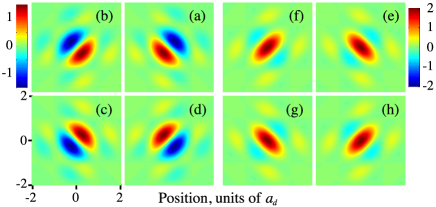
Figure 2: (a)-(d) Spatial dependence of the phase spread functions $a_{i}^{2}P_{\varphi}({\bf r},z=0)$ in quadrants 1-4, respectively; (e)-(h) the intensity spread functions $a_{i}^{2}P_{\alpha}({\bf r},z=0)$ in quadrants 1-4, respectively. The functions are calculated for the in-focus position $z=0$ and detection aperture ${\rm NA_{d}}=2{\rm NA_{i}}$. Lateral positions are in units of $a_{d}$.

Eqs. (19) and (20) are some of the main results of this work. Though we have taken as examples square apertures here, they are valid for arbitrary shapes of the detection and illumination apertures and for arbitrary defocus positions $z$.

4.1 Phase-gradient expansion

In the limit of small wavevectors ${\bf k}\to 0$ we recover the approximation of smooth phase gradients (7). Indeed, since our optical system can only detect variations of phase, the zero frequency term of Eq. (20), corresponding to a constant phase, vanishes, $\tilde{P}_{\varphi}({\bf k}=0,z)=0$. The first non-vanishing term is obtained by Taylor expanding (19) and (20) at small spatial frequencies, leading to

$$I_{d}({\bf r}) \approx \frac{I_{0}}{f_{c}^{2}\Omega_{c}}\int{\rm d^{2}}{\bf r}^{\prime}\left|{\rm A_{d}}\left(\frac{f_{e}}{f_{c}}{\bf r}^{\prime}-{\bf b}\right)\right|^{2}$$ (21)

$$\times\left[1-2\alpha({\bf r})-\frac{f_{c}}{2\pi k}\nabla_{{\bf r}}\varphi({\bf r})\nabla_{{\bf r}^{\prime}}\right]{\rm A_{c}}\left(-{\bf r}^{\prime}\right),$$

which, in fact, is the Taylor expansion of Eq. (7) in the limit of small phase gradients (see details in Appendix). Specifically, when a square illumination aperture is smaller than the detection aperture of each lens of a quatrefoil assembly (8), we obtain the small phase-gradient approximation of Eq. (9)

$$I_{d}({\bf r})\approx\frac{I_{0}}{4}\left[1-2\alpha({\bf r})\pm\frac{a_{i}}{\pi}\partial_{x}\varphi({\bf r})\pm\frac{a_{i}}{\pi}\partial_{y}\varphi({\bf r})\right].$$ (22)

The phase gradients are orthogonal here to the edges of illumination aperture. As before, the signs of phase gradients are defined by the detection lens quadrant. Phase gradients are obtained using the linear combinations of intensities (3.1).

5 In-focus phase imaging

The range of spatial frequencies where Eq. (12) remains valid can be estimated by studying the structure of the phase transfer function (20) beyond the Taylor expansion. We assume that a phase sample is located at the focal plane $z=0$ and consider a square illumination aperture that is smaller than the detection aperture of each lens in a quatrefoil assembly (8). As an example, we assume that the detection aperture is a square of size $2d_{p}\times 2d_{p}$. The corresponding numerical aperture is given by ${\rm NA_{d}}=d_{p}/f_{e}$.

Having derived the transfer functions (19) and (20), we can now refine our phase imaging method (12). Previously we made use of Eq. (10) to relate local light tilts to sample phase variations. Here, we formally define light tilts according to Eq. (3.1) and derive the relations between the tilts and phase

$$\theta_{x}({\bf r}) = {\rm NA_{i}}\int{\rm d^{2}}{\bf r}_{0}\,P^{x}_{\theta}({\bf r}-{\bf r}_{0})\varphi({\bf r}_{0}),$$

$$\theta_{y}({\bf r}) = {\rm NA_{i}}\int{\rm d^{2}}{\bf r}_{0}\,P^{y}_{\theta}({\bf r}-{\bf r}_{0})\varphi({\bf r}_{0}).$$ (23)

The spread functions of the tilts are linear combinations of the spread functions of intensities $P^{(m)}_{\varphi}({\bf r})$, where $m=1..4$ identifies the quadrant of the lens assembly:

$$P^{x}_{\theta} = P^{(1)}_{\varphi}+P^{(4)}_{\varphi}-P^{(2)}_{\varphi}-P^{(3)}_{\varphi},$$

$$P^{y}_{\theta} = P^{(1)}_{\varphi}+P^{(2)}_{\varphi}-P^{(3)}_{\varphi}-P^{(4)}_{\varphi}.$$ (24)

The transfer functions of the tilts $\tilde{P}^{x}_{\theta}({\bf k})$ and $\tilde{P}^{y}_{\theta}({\bf k})$ at the in-focus position $z=0$ are obtained by substituting Eq. (15) in (3.1) and using the Fourier transform:

$$\tilde{\theta}_{x}({\bf k})={\rm NA_{i}}\tilde{P}^{x}_{\theta}({\bf k})\tilde{\varphi}({\bf k}),\quad\tilde{\theta}_{y}({\bf k})={\rm NA_{i}}\tilde{P}^{y}_{\theta}({\bf k})\tilde{\varphi}({\bf k}),$$ (25)

We substitute Eq. (20) into Fourier-transformed Eqs. (3.1) and derive separable representations

$$\tilde{P}^{x}_{\theta}({\bf k})=2i\,\tilde{g}_{-}(k_{x})\tilde{g}_{+}(k_{y}),\quad\tilde{P}^{y}_{\theta}({\bf k})=2i\,\tilde{g}_{-}(k_{y})\tilde{g}_{+}(k_{x}),$$ (26)

where the functions $\tilde{g}_{-}(q)$ and $\tilde{g}_{+}(q)$ are illustrated in Fig. 3 and explicitly expressed in Appendix.

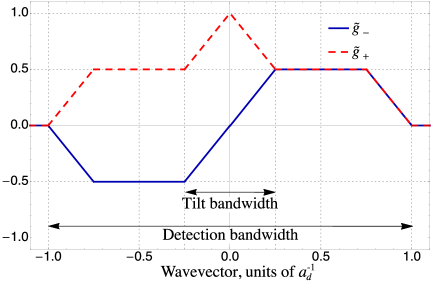
Figure 3: Plots of $\tilde{g}_{-}$ and $\tilde{g}_{+}$ for in-focus imaging when the detection aperture is a square and ${\rm NA_{d}}=2{\rm NA_{i}}$.

We can understand the behavior of these functions qualitatively, again from Fig. 1(b). Specifically, the function $\tilde{g}_{-}(q)$ is proportional to the tilt angle along one direction. Let us consider a prism-like sample that refracts light along $y$-axis. A positive tilt is imposed by the prism $\theta_{y}=k_{y}/k\geq 0$ along $y$-axis. When the tilt is relatively small, the image shifts upwards, and the two upper lenses of the quatrefoil assembly collect more light than the lower ones. Correspondingly, function $\tilde{g}_{-}(k_{y})$ grows linearly with $k_{y}$ until the tilt angle reaches the limiting value of the tilt range, $\theta_{y}={\rm NA_{i}}$. For larger angles, ${\rm NA_{i}}<\theta_{y}\leq{\rm NA_{d}}-{\rm NA_{i}}$, the lower lenses collect no light, while the upper ones collect the maximum power. The power does not change until the image of the illumination aperture reaches the top edge of the lens assembly at $\theta_{y}={\rm NA_{d}}-{\rm NA_{i}}$. Still at larger angles of refraction, the intensity collected by the upper lenses begins to decrease until it falls to zero when the image of illumination aperture leaves the lens assembly altogether at $\theta_{y}={\rm NA_{d}}$. Similar arguments apply to negative tilts $\theta_{y}\leq 0$, and it is straightforward to see that $\tilde{g}_{-}(k_{y})$ is an odd function of $k_{y}$. The optical bandwidth of the system is defined here by the detection aperture, $|k_{x,y}|\leq 1/a_{d}$, where $a_{d}=\lambda/(2{\rm NA_{d}})$. The function $\tilde{g}_{-}$ is shown in Fig. 3.

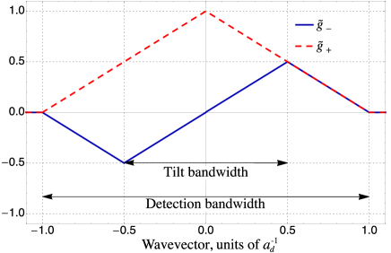
Figure 4: Plots of $\tilde{g}_{-}$ and $\tilde{g}_{+}$ for in-focus imaging when the detection aperture is a square and ${\rm NA_{d}}={\rm NA_{i}}$.

The detection and illumination apertures completely characterize the light-tilt transfer functions. As we discuss below, to achieve detection-limited resolution for imaging out-of-focus phase objects, the numerical apertures of illumination and detection should be matched, ${\rm NA_{i}}={\rm NA_{d}}$. Fig. 4 illustrates the transfer functions in this case. In contrast to Fig. 3, the range of frequencies for which $\tilde{g}_{-}=1/2$ has been reduced to a point.

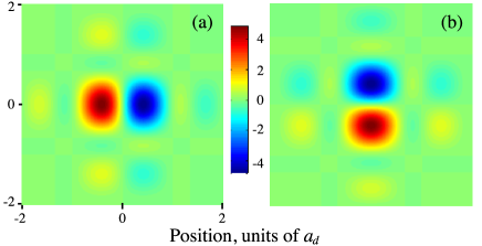
Figure 5: Spatial dependence of the tilt spread functions: $a_{i}^{2}P^{x}_{\theta}({\bf r},z=0)$ (a), and $a_{i}^{2}P^{y}_{\theta}({\bf r},z=0)$ (b), calculated for the in-focus position $z=0$, when the detection aperture is a square and ${\rm NA_{d}}=2{\rm NA_{i}}$. Lateral positions are in units of $a_{d}$.

5.1 Spatial frequencies limited by the illumination aperture

To begin, we consider spatial frequencies within the tilt range of our system, namely $|k_{x,y}|\leq 1/(2a_{i})$, as defined by the illumination numerical aperture. The functions $\tilde{g}_{-}(k_{x,y})=k_{x,y}a_{i}$ and $\tilde{g}_{+}(k_{x,y})=1-|k_{x,y}a_{i}|$ are then independent of the detection aperture. The corresponding Fourier components of the tilts (26) are given by

$$\tilde{\theta}_{x}({\bf k}) = i\frac{k_{x}}{k}(1-|k_{y}a_{i}|)\tilde{\varphi}({\bf k}),$$

$$\tilde{\theta}_{y}({\bf k}) = i\frac{k_{y}}{k}(1-|k_{x}a_{i}|)\tilde{\varphi}({\bf k}),$$ (27)

where $|k_{x,y}|\leq 1/(2a_{i})$. These equations uniquely map the directions of light rays $k_{x,y}/k$ to the tilt angles along the same axes in proportion to the Fourier components of the phase. These may be compared with Eqs. (10) utilized for our smooth phase approximation, and are found to be equivalent except for an additional attenuation of spatial frequencies orthogonal to the tilt directions.

Phase is extracted from (5.1) using a linear combination of the tilts

$$\tilde{\varphi}({\bf k})=-ik\,\frac{\tilde{\theta}_{x}({\bf k})+i\tilde{\theta}_{y}({\bf k})}{k_{x}(1-|k_{y}a_{i}|)+ik_{y}(1-|k_{x}a_{i}|)},$$ (28)

where $|k_{x,y}|\leq 1/(2a_{i})$, or, correspondingly,

$$\varphi({\bf r})=-ik\int{\rm d^{2}}{\bf k}\,e^{i2\pi{\bf k}{\bf r}}\,\frac{\tilde{\theta}_{x}({\bf k})+i\tilde{\theta}_{y}({\bf k})}{k_{x}(1-|k_{y}a_{i}|)+ik_{y}(1-|k_{x}a_{i}|)},$$ (29)

where integration extends over the tilt range $|k_{x,y}|\leq 1/(2a_{i})$. In this derivation we assumed that the spatial support of $\varphi({\bf r})$ is finite within the imaging field of view. We note that Eq. (29) is applicable to arbitrary shapes of the detection lens provided the associated aperture exceeds the numerical aperture of illumination. The phase reconstruction (29) should be used when the illumination aperture is well characterized, while the detection aperture is not precisely known. However, the method does not account for the spatial frequencies beyond the tilt range.

5.2 Spatial frequencies limited by the detection aperture

The resolution of phase reconstruction can be improved if the detection aperture is precisely known. We use the known spread functions to deconvolve light tilts and obtain the phase

$$\varphi({\bf r})=\frac{1}{{\rm NA_{i}}}\int{\rm d^{2}}{\bf k}\,e^{i2\pi{\bf k}{\bf r}}\,\frac{\tilde{\theta}_{x}({\bf k})+i\tilde{\theta}_{y}({\bf k})}{\tilde{P}^{x}_{\theta}({\bf k})+i\tilde{P}^{y}_{\theta}({\bf k})},$$ (30)

where integration now extends over the detection bandwidth. For a square detection aperture, the spread functions of light tilts are given in Appendix. Corresponding illustrations of the tilt spread functions $P^{x}_{\theta}({\bf r})$ and $P^{y}_{\theta}({\bf r})$ are shown in Fig. 5 for the in-focus position $z=0$. As can be observed, $P^{x}_{\theta}({\bf r})$ is even with respect to $y$-axis and odd with respect to $x$-axis, and for the function $P^{y}_{\theta}({\bf r})$ vice-versa.

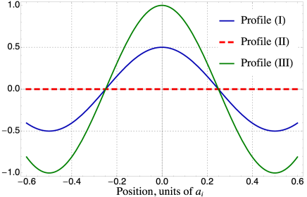
Figure 6: Reconstruction of a periodic phase profile $\varphi(x)/\varphi_{0}$ in Eq. (31) when $Q=1/a_{i}$ and ${\rm NA_{d}}=2{\rm NA_{i}}$ using different methods: Eq. (12) (solid blue line), Eq. (29) (red dashed line), and Eq. (30) (green solid line). The exact profile is depicted by the green solid line. Lateral position is in units of $a_{i}$.

Let us compare the reconstruction methods (12), (29) and (30) in the simple case of a one-dimensional periodic phase profile

$$\varphi(x)=\varphi_{0}\cos(2\pi Qx),$$ (31)

where $Q\geq 0$ is the periodic spatial frequency. It is easy to verify that when $Q\leq 1/(2a_{i})$ different phase reconstruction methods yield an identical profile $\varphi_{rec}(x)=\varphi(x)$. However, for larger frequencies the reconstructions are different. We consider for example frequencies within the range $1/(2a_{i})\leq Q\leq 1/a_{d}-1/a_{i}$. The tilt transfer function is then constant $\tilde{g}_{-}(\pm Q)=\pm 1/2$ (see Fig. 3). The reconstruction results are summarized in Fig. 6, where ${\rm NA_{d}}=2{\rm NA_{i}}$ and frequency $Q=1/a_{i}$. According to Eq. (12) we obtain $\varphi_{rec}(x)=\psi\cos(2\pi Qx)$, where the reconstructed amplitude $\psi=\varphi_{0}/(2a_{i}Q)$ incorrectly depends on the spatial frequency $Q$ instead of being the constant $\varphi_{0}$ (Profile (I) in Fig. 6). This inconsistency is due to the incorrect mapping of phase to tilts outside of the tilt range. A refined approach (29) is only sensitive to spatial frequencies within the tilt range, so when $Q>1/(2a_{i})$, the reconstructed profile $\varphi_{rec}(x)=0$ (Profile (II) in Fig. 6) is also incorrect. Finally, Eq. (30) properly accounts for all spatial frequencies within the detection bandwidth $Q\leq 1/a_{d}$, and, as a result, provides the correct reconstruction of the original profile $\varphi_{rec}(x)=\varphi(x)$ (Profile (III) in Fig. 6). Thus all the spatial frequency components of an arbitrary phase profile within the detection bandwidth can, in principle, be found using Eq. (30). Approximate reconstructions of phase samples characterized by even broader spatial frequency distributions are also possible, as we discuss below.

The phase reconstruction methods (29) and (30) are the main results of this work. Experiments reported in Refs. [18, 19] employed the simplified method (12) of phase reconstruction. Since the spatial frequencies of the imaged samples were safely confined to the tilt range, the reconstruction (12) provided good approximations of phase profiles.

5.3 Imaging a phase step

It is instructive to apply the above formalism to the imaging of a phase, which manifestly is not smooth and features high spatial frequencies. The strong light diffraction from the discontinuity allows to visualize spatial resolution of our phase imaging method. For simplicity we consider a one-dimensional step

$$\varphi({\bf r})=\varphi_{0}\,{\rm H}(x),$$ (32)

where the amplitude is small, $|\varphi_{0}|\ll 1$, and the Heaviside function ${\rm H}(x)=1$ at $x\geq 0$, and ${\rm H}(x)=0$ at $x<0$.

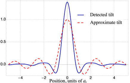
Figure 7: Detected and approximate light tilts $\theta_{x}/\theta_{0}$ as a function of position when imaging a phase step (32)and in the case of matched numerical apertures ${\rm NA_{d}}={\rm NA_{i}}$. Lateral position is in units of $a_{i}$.

The Fourier components $\tilde{\varphi}({\bf k})$ are calculated using standard regularization, in which we add an infinitesimal imaginary part to the wavevector $k_{x}\to k_{x}-i0$

$$\tilde{\varphi}({\bf k})=\frac{\varphi_{0}}{2\pi i(k_{x}-i0)}\delta(k_{y}).$$ (33)

The Fourier components of the detected light tilts (3.1) resulting from the object are limited by the detection aperture

$$\tilde{\theta}_{x}({\bf k})=\theta_{0}\frac{\tilde{g}_{-}(k_{x})}{k_{x}}\delta(k_{y}),\quad\tilde{\theta}_{y}({\bf k})=0,\quad|k_{x}|\leq 1/a_{d},$$ (34)

where we define the light tilt $\theta_{0}=(\varphi_{0}/\pi){\rm NA_{i}}$. The discontinuity (33) diffracts light in all directions along $x$-axis, and the detection aperture collects only part of this light.

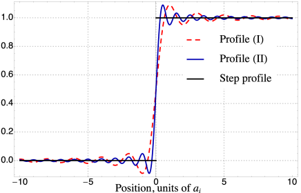
Figure 8: Step profiles $\varphi(x)/\varphi_{0}$ reconstructed using Eq. (12) (Profile I, red dashed line), and Eq. (29) (Profile II, solid blue line), with detection aperture ${\rm NA_{d}}={\rm NA_{i}}$. The profiles approximate a step function (32) shown as in solid black. Lateral position is in units of $a_{d}$.

In real space the detected tilt angle becomes

$$\theta_{x}(x)=\theta_{0}\int_{-1/a_{d}}^{1/a_{d}}{\rm d}k_{x}\,e^{i2\pi k_{x}x}\tilde{g}_{-}(k_{x})/k_{x},\quad\theta_{y}({\bf r})=0.$$ (35)

The dependence of the detected light tilt on the position along $x$-axis is plotted as a solid blue line in Fig. 7, assuming a square detection aperture of numerical aperture ${\rm NA_{d}}={\rm NA_{i}}$. For comparison we also plot an approximate tilt (dashed red line) given by $\theta_{x}(x)=\theta_{0}\,{\rm sinc}(\pi x/a_{i})$, which is obtained from the detected tilt (34) by setting to zero the spatial frequencies $|k_{x}|\geq 1/(2a_{i})$. We interpret the peak of the approximate tilt as follows. As a light ray refracts from the step, it effectively traverses an optical path $h=\varphi_{0}\lambda/(2\pi)$ within a lateral spot of size estimated by the resolution scale $a_{i}=\lambda/(2{\rm NA_{i}})$. The effective angle of refraction (i.e. tilt) is then estimated as the ratio of the optical path to the spot size, $\theta=h/a_{i}$, which coincides with the peak value $\theta_{0}=(\varphi_{0}/\pi){\rm NA_{i}}$ of the approximate tilt. The detected tilt (shown in blue solid line) is obtained similarly using the detection-limited resolution. Therefore, the peak detected tilt is expected to be proportionally larger. However, since the transfer function $\tilde{g}_{-}$ in Fig. (4) is not linear, the peak value of the detected tilt is only somewhat larger than the peak of the approximate tilt.

Results of phase reconstruction are summarized in Fig. 8. All reconstruction methods define the phase profiles up to an arbitrary constant, which we choose to be $\varphi(0)=\varphi_{0}/2$. The low-frequency part of the tilt $\tilde{\theta}_{x}({\bf k})=\theta_{0}a_{i}\delta(k_{y})$ valid within the tilt range $|k_{x}|\leq 1/(2a_{i})$, is employed in the reconstruction (29). The corresponding profile (I) is $\varphi(x)/\varphi_{0}=1/2+(1/\pi){\rm Si}(\pi x/a_{i})$, where ${\rm Si}(z)=\int_{0}^{z}{\rm d}q\sin(q)/q$, shown as a dashed red line. The oscillations near the discontinuity $x=0$, known as the Gibbs phenomenon, are attributed to the finite range $|k_{x}|\leq 1/(2a_{i})$ of the integration in (29). The reconstruction (30) is given by $\varphi(x)/\varphi_{0}=1/2+(1/\pi){\rm Si}(2\pi x/a_{i})$, and plotted as the solid blue line Profile (II). We note that in the considered case $a_{i}=a_{d}$. The oscillations around the step identify the spatial resolution of our system since they are a result of the finite detection bandwidth. Naturally, as the detection bandwidth is increased, the profile approaches the step function.

6 Out-of-focus phase imaging

In this section we analyze phase imaging of out-of-focus objects located a distance $z$ from the focal plane. The acquired images in this case exhibit both blurring and quadrant-dependent lateral shearing compared to in-focus imaging. As in light field imaging [22], we make use of the fact that shearing provides information on the defocus position and can be compensated for. The blurring of images for large defocus, however, cannot be compensated and degrades spatial resolution. We show that out-of-focus phase profiles can nevertheless, in principle, be reconstructed, though with a reduced spatial resolution depending on the extent of defocus.

The exact relation between the numerical apertures of illumination and detection is not critical for phase reconstruction of in-focus objects, provided the detection aperture is accurately known. For defocused objects the situation is different, since the two apertures both control the effects of blurring and shearing. The case of matched numerical apertures ${\rm NA_{i}}={\rm NA_{d}}$ is special, since in that case lateral shearing observed in different quadrants at the optical resolution uniquely identifies the defocus distance (see below and also Appendix). In the unbalanced case ${\rm NA_{i}}<{\rm NA_{d}}$, the situation is more complicated. The problem comes from the spectral components of intensities outside the tilt bandwidth, since they shear differently than the spectral components within the bandwidth. That is why, we consider only the frequencies within the detection bandwidth $|k_{x,y}|\leq 1/(2a_{i})$, which can be accomplished by applying a low-pass filter to the recorded images. The formalism presented below concentrates on the detection-limited phase reconstruction for a system with matched numerical apertures. However, it can also be applied in the unbalanced case after numerically filtering the bandwidth of the recorded images to be within the tilt bandwidth (see also Section 9.8 in Appendix).

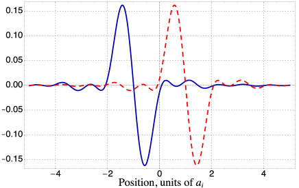
Figure 9: Averaged phase spread functions, $a_{i}\langle P_{\varphi}^{(1)}(x,y)\rangle_{y}$ (solid blue line) and the negative of $a_{i}\langle P_{\varphi}^{(2)}(x,y)\rangle_{y}$ (dashed red line), calculated in quadrants (1) and (2), as functions of lateral position $x$ at the defocus position $z=z_{i}$, in the case of matched numerical apertures ${\rm NA_{i}}={\rm NA_{d}}$. The two functions are replicas of one another, shifted by $\Delta x=2{\rm NA_{i}}z$. Lateral position is in units of $a_{i}$.

The principle of numerical refocusing is illustrated in Fig. 9, where we considered the case of matched numerical apertures ${\rm NA_{i}}={\rm NA_{d}}$. We find that defocused spread functions of quadrants (1) and (2) averaged over the $y$ coordinate, $\langle P_{\varphi}^{(1)}(x,y,z)\rangle_{y}$ and $\langle P_{\varphi}^{(2)}(x,y,z)\rangle_{y}$, are replicas of one another shifted along $x$-axis, up to a negative sign. Since the intensity of an image is obtained as a convolution (17) of phase and the phase spread function, we observe that the images of an arbitrary phase object shift accordingly. The relative shift is proportional to the defocus distance, $\Delta x=2{\rm NA_{i}}z$, and, thus, unambiguously identifies this distance.

In the two-dimensional case, to avoid ambiguities, we also need to consider the first and fourth quadrants, and average the corresponding phase-sensitive intensities over the $x$ coordinate. The averaged intensities depending on coordinate $y$ are the shifted replicas of one another, up to a negative sign. The two relations between the intensities are given by

$$\langle I^{(1)}_{\varphi}(x-{\rm NA_{i}}z,y)\rangle_{y} = -\langle I^{(2)}_{\varphi}(x+{\rm NA_{i}}z,y)\rangle_{y},$$

$$\langle I^{(1)}_{\varphi}(x,y-{\rm NA_{i}}z)\rangle_{x} = -\langle I^{(4)}_{\varphi}(x,y+{\rm NA_{i}}z)\rangle_{x},$$ (36)

where $\langle..\rangle_{x,y}$ is the average over coordinates $x$ and $y$, respectively, and $I^{(m)}_{\varphi}({\bf r})$ is a phase-sensitive part of the intensity recorded in quadrant $m$. The intensity $I^{(m)}_{\varphi}({\bf r})$ is obtained by subtracting the background from the total intensity (15). Identities (6) provide, in principle, an estimate of the defocus position $z$, for example, by maximizing the cross-correlation function of the averaged intensities.

Light tilts adjusted for the shearing are given by

$$\theta_{x}({\bf r},z) = \frac{{\rm NA_{i}}}{I_{tot}}\left[\begin{array}[]{ll}I_{1}(x_{-},y_{-})+I_{4}(x_{-},y_{+})\\ -I_{2}(x_{+},y_{-})-I_{3}(x_{+},y_{+})\end{array}\right],$$ (39)

$$\theta_{y}({\bf r},z) = \frac{{\rm NA_{i}}}{I_{tot}}\left[\begin{array}[]{ll}I_{1}(x_{-},y_{-})+I_{2}(x_{-},y_{+})\\ -I_{3}(x_{+},y_{-})-I_{4}(x_{+},y_{+})\end{array}\right],$$ (42)

where $x_{\pm}=x\pm{\rm NA_{i}}z$, $y_{\pm}=y\pm{\rm NA_{i}}z$, $I_{m}({\bf r})$ is the intensity recorded in quadrant $m$, and $I_{tot}=I_{1}(x_{-},y_{-})+I_{2}(x_{-},y_{+})+I_{3}(x_{+},y_{-})+I_{4}(x_{+},y_{+})$.

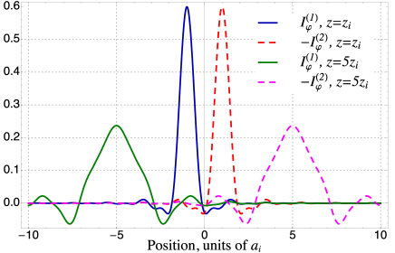
Figure 10: Intensities $I^{(1)}_{\varphi}(x,z)$ and negative $I^{(2)}_{\varphi}(x,z)$ as functions of lateral position $x$, calculated for different defocus distances and with matched numerical apertures ${\rm NA_{i}}={\rm NA_{d}}$. Solid blue line and dashed red line correspond to $z=z_{i}$; solid green line and dashed magenta line correspond to $z=5z_{i}$. Lateral position is in units of $a_{i}$.

We find the Fourier components of (39) and use the known transfer functions of tilts (9.6) (see Appendix) to obtain the phase of an out-of-focus object

$$\varphi({\bf r},z)=\frac{1}{{\rm NA_{i}}}\int{\rm d^{2}}{\bf k}\,e^{i2\pi{\bf k}{\bf r}}\,\frac{\tilde{\theta}_{x}({\bf k},z)+i\tilde{\theta}_{y}({\bf k},z)}{\tilde{P}^{x}_{\theta}({\bf k},z)+i\tilde{P}^{y}_{\theta}({\bf k},z)},$$ (43)

where the integration extends over the detection bandwidth $|k_{x,y}|\leq 1/a_{i}$, when the numerical apertures of illumination and detection match, ${\rm NA_{i}}={\rm NA_{d}}$ (i.e. $a_{d}=a_{i}$). We note that for relatively small defocus, deconvolution is in principle possible within the detection bandwidth, based on the transfer functions (9.6). In cases when ${\rm NA_{i}}<{\rm NA_{d}}$ the integration extends over the tilt bandwidth $|k_{x,y}|\leq 1/(2a_{i})$, which leads to a reduced spatial resolution compared to the case of matched apertures. For a relatively large defocus, the combination of transfer functions in (43) has zeros at $k_{x,y}\neq 0$. The bandwidth should be reduced to exclude these singularities from the integration. The appearance of singularities identifies the defocus regime where the blurring cannot be accurately compensated, which results in reduced resolution of phase reconstruction depending on the defocus distance.

6.1 Imaging a defocused phase step

We illustrate reconstruction (43) of a defocused phase step (32) by a system with matched numerical apertures ${\rm NA_{i}}={\rm NA_{d}}$. Intensities detected in the first and second quadrants are obtained using the transfer functions (67). The characteristic axial length scale of defocusing is the depth of focus $z_{i}=\lambda/(2{\rm NA_{i}^{2}})$. Intensities calculated at $z=z_{i}$ and $z=5z_{i}$ are shown in Fig. 10. From these plots we can unambiguously identify the defocus positions. Indeed, pairs of intensities calculated at the axial positions $z=z_{i}$ and $z=5z_{i}$ are shifted with respect to one another by distances $\delta x=2a_{i}$ and $\delta x=10a_{i}$, respectively. Phase profiles reconstructed according to Eq. (43) are demonstrated in Fig. 11. We choose an arbitrary constant so that $\varphi(0)=\varphi_{0}/2$. The reconstructed profile $\varphi(x)/\varphi_{0}=1/2+(1/\pi){\rm Si}(2\pi x/a_{i})$ calculated at $z=z_{i}$ is identical to the in-focus one. One can show that detection-limited phase reconstruction is possible for relatively small defocus $|z|<2z_{i}$. In contrast, the profile reconstructed at $z=5z_{i}$ is characterized by a reduced spatial resolution. The reason is that at this relatively large defocus the transfer function $\tilde{P}^{x}_{\theta}(k_{x},z)=0$ at $|k_{x}|=k_{c}=0.32/a_{i}$ within the detection bandwidth $|k_{x}|\leq 1/a_{i}$. To avoid the singularities in (43), we thus restrict the bandwidth of integration to a smaller range $|k_{x}|<k_{c}$. The resulting profile is given by $\varphi(x)/\varphi_{0}=1/2+(1/\pi){\rm Si}(2\pi xk_{c})$. Oscillations observed around discontinuity at $x=0$ are due to the limited bandwidth of integration in (43). As the defocus distance is increased, the integration bandwidth is gradually reduced. We find that even at a significant defocus distance $z=20z_{i}$, the first zero of the tilt transfer function occurs at $k_{c}=0.16/a_{i}$, so that the bandwidth is reduced only two times compared to $z=5z_{i}$.

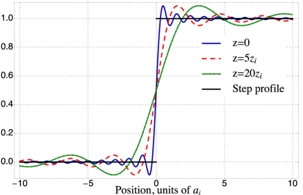
Figure 11: Phase profiles $\varphi(x)/\varphi_{0}$ of a step (32), depicted by in solid black, reconstructed according to Eq. (43): the solid blue line corresponds to $z=z_{i}$, dashed red line corresponds to $z=5z_{i}$. Lateral position is in units of $a_{i}$.

7 Conclusion

In this work we considered quantitative phase imaging using a partitioned detection aperture microscope introduced in Ref. [18]. Our single-exposure method is characterized by a simple optical design that is light efficient and insensitive to polarization. The microscope may be implemented in transmission or reflection modes [18, 19]. Within the wave-optic paraxial approximation we derived the three-dimensional spread functions of intensity and phase (19) and (20), analyzed their properties, and refined the phase-imaging approach of Ref. [18, 19], making it suitable for imaging smooth and rough samples. The formalism is summarized in Eq. (30). In particular, we demonstrated that the spatial resolution of our method is limited by the detection aperture in contrast to Refs. [18, 19] where the resolution was defined by a smaller tilt range. We also showed how our method reconstructs the profile of a phase step provided is optical path-length is smaller than the wavelength. Further, we extended the method to imaging of defocused phase objects, as described in Eqs. (6), (39) and (43). Even for relatively large object defocus, the method provides precise reconstructions of rough and smooth samples with spatial resolution depending on the defocus distance.

8 Acknowledgments

Financial support for this work was partially provided by NIH CA182939.

9 Appendix

We provide calculations of spread functions, which, for the sake of clarity, were omitted in the main text.

In our calculations we employ the following convention for Fourier transforms

$$f({\bf r})=\int{\rm d^{2}}{\bf k}\,e^{i2\pi{\bf k}{{\bf r}}}\tilde{f}({\bf k}),\quad\tilde{f}({\bf k})=\int{\rm d^{2}}{{\bf r}}\,e^{-i2\pi{\bf k}{{\bf r}}}f({{\bf r}}).$$ (44)

9.1 Phase-gradient expansion of transfer functions

In the limit of small wavevectors ${\bf k}\to 0$, one can simplify (20). Assuming that the aperture is a real function, ${\rm A^{*}_{c}}={\rm A_{c}}$, we expand the difference of the functions into the Taylor series and keep the first non-vanishing term

$${\rm A_{c}}\left(-\frac{f_{c}}{k}{\bf q}_{+}\right)-{\rm A^{*}_{c}}\left(-\frac{f_{c}}{k}{\bf q}_{-}\right)\approx{\bf k}\,\nabla_{{\bf q}}{\rm A_{c}}\left(-\frac{f_{c}}{k}{\bf q}\right),$$ (45)

where ${\bf q}_{\pm}={\bf q}\pm{\bf k}/2$. Substituting this expression in Eq. (20), and restricting the expansions to terms linear in ${\bf k}$, we derive an approximate phase transfer function

$$\tilde{P}_{\varphi}({\bf k},z) \approx -\frac{i}{f_{c}\Omega_{c}k}\int{\rm d^{2}}{\bf r}^{\prime}\left|{\rm A_{d}}\left(\frac{f_{e}}{f_{c}}{\bf r}^{\prime}-{\bf b}\right)\right|^{2}$$ (46)

$$\times\,{\bf k}\nabla{\rm A_{c}}\left(-{\bf r}^{\prime}\right),$$

where we introduced the integration variable ${\bf r}=(f_{c}/k){\bf q}$. The Fourier components of the function are most significant along the directions of rapid variations of the illumination aperture. For a uniformly illuminated aperture, the directions are orthogonal to the aperture edge.

The intensity transfer function (19) is approximated by its value at ${\bf k}=0$ given by

$$\tilde{P}_{\alpha}({\bf k}=0,z)=\frac{2}{f^{2}_{c}\Omega_{c}}\int{\rm d^{2}}{\bf r}^{\prime}\,\left|{\rm A_{d}}\left(\frac{f_{e}}{f_{c}}{\bf r}^{\prime}-{\bf b}\right)\right|^{2}{\rm A_{c}}\left(-{\bf r}^{\prime}\right).$$ (47)

The next non-vanishing order of $\tilde{P}_{\alpha}({\bf k},z)$ scales as ${\bf k}^{2}$ and can be neglected, since we limit the expansions to terms linear in ${\bf k}$.

Substituting the transfer functions (46) and (47) in Eq. (18), and performing the inverse Fourier transform, we obtain the intensity at the detector plane (21).

9.2 Spread functions for intensity and phase

Below we define the spread functions of phase, tilt angles and intensity when the detection aperture is a square. We assume that ${\rm NA_{d}}\geq{\rm NA_{i}}$. In the following, to simplify the notations we use the dimensionless coordinates

$$z/z_{i}\to z,\quad{\bf r}/a_{i}\to{\bf r},$$ (48)

where $a_{i}=\lambda/(2{\rm NA_{i}})$, and $z_{i}=\lambda/(2{\rm NA^{2}_{i}})$ define the lateral and axial spatial scales, identified as the lateral resolution and the depth of focus of the illumination aperture, respectively. Wavevectors are also rescaled: ${\bf k}a_{i}\to{\bf k}$.

Calculation of the spread functions is relatively straightforward and somewhat tedious, and we provide the results without detailed derivations.

9.3 The intensity spread function

Due to the square symmetry of the illumination aperture, the intensity transfer functions $P^{(m)}_{\alpha}({\bf r})$ (19), where $m$ identifies the quadrant of the detection lens, are given by

$$\tilde{P}^{(m)}_{\alpha}=\frac{1}{4}\left\{\begin{array}[]{ll}\tilde{g}(k_{x},z)\tilde{g}(k_{y},z)+\tilde{g}^{*}(-k_{x},z)\tilde{g}^{*}(-k_{y},z),&\mbox{m=1,}\\ \tilde{g}(-k_{x},z)\tilde{g}(k_{y},z)+\tilde{g}^{*}(k_{x},z)\tilde{g}^{*}(-k_{y},z),&\mbox{m=2,}\\ \tilde{g}(-k_{x},z)\tilde{g}(-k_{y},z)+\tilde{g}^{*}(k_{x},z)\tilde{g}^{*}(k_{y},z),&\mbox{m=3,}\\ \tilde{g}(k_{x},z)\tilde{g}(-k_{y},z)+\tilde{g}^{*}(-k_{x},z)\tilde{g}^{*}(k_{y},z),&\mbox{m=4},\end{array}\right.$$ (49)

where where we defined a piece-wise complex-valued function

$$\tilde{g}(q,z)=\frac{e^{-i2\pi zq^{2}}}{i2\pi zq}\left\{\begin{array}[]{ll}e^{i2\pi zq}-e^{i4\pi zq^{2}},&\mbox{$0\leq q<1/2$},\\ e^{i2\pi zq}-1,&\mbox{$1/2-\beta\leq q<0$,}\\ e^{i4\pi zq(q+\beta)}-1,&\mbox{$-\beta\leq q<1/2-\beta$,}\\ 0,&\mbox{$q<-\beta$, or $q\geq 1/2$},\end{array}\right.$$ (50)

the parameter $\beta={\rm NA_{d}}/{\rm NA_{i}}\geq 1$, and $\tilde{g}^{*}(q,z)$ is the complex conjugate of $\tilde{g}(q,z)$. The real and imaginary parts of $\tilde{g}(q,z)$ are plotted in Fig. 12 when ${\rm NA_{d}}=2{\rm NA_{i}}$ for in-focus and out-of-focus imaging at $z=z_{i}$.

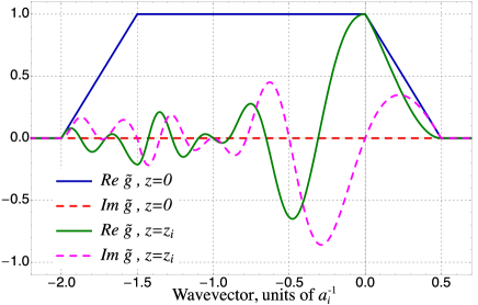
Figure 12: Plots of the function $\tilde{g}(q,z)$ at different defocus distances and in the case ${\rm NA_{d}}=2{\rm NA_{i}}$. Solid blue and red dashed lines depict the real and imaginary parts of $\tilde{g}(q,z)$, respectively, calculated at $z=0$; solid green and dashed magenta lines depict the real and imaginary parts of $\tilde{g}(q,z)$ calculated at $z=z_{i}$.

The real-space representation of this function is simplified at the in-focus position $z=0$

$$g(x,0)=\beta\,e^{-i\pi x(\beta-1/2)}{\rm sinc}\left(\pi x/2\right){\rm sinc}\left(\pi x\beta\right).$$ (51)

The in-focus ($z=0$) intensity spread functions are given by

$$P^{(m)}_{\alpha}({\bf r})=\rho({\bf r})\left\{\begin{array}[]{ll}\cos\left[\pi(x+y)(\beta-1/2)\right],&m=1,\\ \cos\left[\pi(-x+y)(\beta-1/2)\right],&m=2,\\ \cos\left[\pi(-x-y)(\beta-1/2)\right],&m=3,\\ \cos\left[\pi(x-y)(\beta-1/2)\right],&m=4,\end{array}\right.$$ (52)

where $\rho({\bf r})=(\beta^{2}/2){\rm sinc}(\pi x/2){\rm sinc}(\pi y/2){\rm sinc}(\pi x\beta){\rm sinc}(\pi y\beta)$. The intensity spread functions calculated at the in-focus position $z=0$ for different quadrants are plotted in Fig. 2.

9.4 The spread functions for phase and light tilts

Due to the square symmetry of the detection and illumination apertures, the phase transfer functions $\tilde{P}^{(m)}_{\varphi}({\bf k},z)$ (20), where $m$ identifies the quadrant of the lens, are given by

$$\tilde{P}^{(m)}_{\varphi}=-\frac{i}{4}\left\{\begin{array}[]{ll}\tilde{g}(k_{x},z)\tilde{g}(k_{y},z)-\tilde{g}^{*}(-k_{x},z)\tilde{g}^{*}(-k_{y},z),&\mbox{m=1,}\\ \tilde{g}(-k_{x},z)\tilde{g}(k_{y},z)-\tilde{g}^{*}(k_{x},z)\tilde{g}^{*}(-k_{y},z),&\mbox{m=2,}\\ \tilde{g}(-k_{x},z)\tilde{g}(-k_{y},z)-\tilde{g}^{*}(k_{x},z)\tilde{g}^{*}(k_{y},z),&\mbox{m=3,}\\ \tilde{g}(k_{x},z)\tilde{g}(-k_{y},z)-\tilde{g}^{*}(-k_{x},z)\tilde{g}^{*}(k_{y},z),&\mbox{m=4},\end{array}\right.$$ (53)

where the function $\tilde{g}(q,z)$ is defined in Eq. (50).

The in-focus phase spread functions are thus given by

$$P^{(m)}_{\varphi}=-\rho({\bf r})\left\{\begin{array}[]{ll}\sin\left[\pi(x+y)(\beta-1/2)\right],&m=1,\\ \sin\left[\pi(-x+y)(\beta-1/2)\right],&m=2,\\ \sin\left[\pi(-x-y)(\beta-1/2)\right],&m=3,\\ \sin\left[\pi(x-y)(\beta-1/2)\right],&m=4,\end{array}\right.$$ (54)

where $\rho({\bf r})=(\beta^{2}/2){\rm sinc}(\pi x/2){\rm sinc}(\pi y/2){\rm sinc}(\pi x\beta){\rm sinc}(\pi y\beta)$. The phase spread functions at the in-focus position $z=0$ for different quadrants are plotted in Fig. 2.

The in-focus tilt transfer functions are calculated as linear combinations of the phase spread functions according to Eq. (3.1)

$$\tilde{P}^{x}_{\theta} = \tilde{P}_{\varphi}^{(1)}+\tilde{P}_{\varphi}^{(4)}-\tilde{P}_{\varphi}^{(2)}-\tilde{P}_{\varphi}^{(3)},$$

$$\tilde{P}^{y}_{\theta} = \tilde{P}_{\varphi}^{(1)}+\tilde{P}_{\varphi}^{(2)}-\tilde{P}_{\varphi}^{(3)}-\tilde{P}_{\varphi}^{(4)}.$$ (55)

Taking the limit $z\to 0$ in Eqs. (53) and substituting the result into (9.4), we obtain

$$\tilde{P}^{x}_{\theta}({\bf k})=2i\,\tilde{g}_{-}(k_{x})\tilde{g}_{+}(k_{y}),\quad\tilde{P}^{y}_{\theta}({\bf k})=2i\,\tilde{g}_{-}(k_{y})\tilde{g}_{+}(k_{x}),$$ (56)

where

$$\tilde{g}_{-}(q) = \left[\tilde{g}(-q,0)-\tilde{g}(q,0)\right]/2,$$

$$\tilde{g}_{+}(q) = \left[\tilde{g}(-q,0)+\tilde{g}(q,0)\right]/2.$$ (57)

The functions $\tilde{g}_{-}(q)$ and $\tilde{g}_{+}(q)$ are the odd and even functions, respectively. For positive arguments, the functions are

$$\tilde{g}_{-}(q)=\left\{\begin{array}[]{ll}q,&\mbox{if $0\leq q<1/2$,}\\ 1/2,&\mbox{$1/2\leq q<\beta-1/2$,}\\ \beta-q,&\mbox{$\beta-1/2\leq q<\beta$,}\\ 0,&\mbox{$q\geq\beta$,}\end{array}\right.$$ (58)

$$\tilde{g}_{+}(q)=\left\{\begin{array}[]{ll}1-q,&\mbox{$0\leq q<1/2$,}\\ 1/2,&\mbox{$1/2\leq q<\beta-1/2$,}\\ \beta-q,&\mbox{$\beta-1/2\leq q<\beta$,}\\ 0,&\mbox{$q\geq\beta$.}\end{array}\right.$$ (59)

The functions are shown in Fig. 3 for the case $\beta=2$, that is when ${\rm NA_{d}}=2{\rm NA_{i}}$.

Real-space representations of the functions are given by

$$g_{+}(x)={\rm Re}\,g(x,0),\quad g_{-}(x)=-i\,{\rm Im}\,g(x,0),$$ (60)

where ${\rm Re}$ and ${\rm Im}$ are the real and imaginary parts, respectively, and the function $g(x,0)$ is defined in Eq. (51).

The tilt spread functions are the products of the functions

$$P^{x}_{\theta}({\bf r})=2i\,g_{-}(x)g_{+}(y),\quad P^{x}_{\theta}({\bf r})=2i\,g_{-}(y)g_{+}(x).$$ (61)

The functions are plotted in Fig. 5 in the case $\beta=2$, that is when ${\rm NA_{d}}=2{\rm NA_{i}}$.

9.5 Properties of the 3D phase spread functions

At a defocus distance $z$, the phase spread functions exhibit lateral shearing and blurring. These effects can be traced to the behavior of the corresponding transfer functions $\tilde{g}(q,z)$ in (50) at different spatial frequencies. For example, within the tilt range $|k_{x,y}|\leq 1/2$ (in dimensionless units), the transfer functions are proportional to the phase factor encoding lateral shearing in real space $\tilde{P}^{(m)}_{\varphi}({\bf k},z)\sim\exp\left[i2\pi(\pm k_{x}\pm k_{y})z\right]$, where the signs depend on the quadrant $m$.

Lateral shearing of the spread functions allows identification of the corresponding defocus position $z$. For simplicity, let us consider the reduced transfer functions in which one of the two components of the wavevector is set to zero. Depending on the value of the remaining second component, the transfer functions are related to one another. For the first and second quadrants we find

$$\tilde{P}_{\varphi}^{(1)}(k_{x},0,z)=-\tilde{P}_{\varphi}^{(2)}(k_{x},0,z)h(k_{x},z),$$ (62)

where

$$h(q,z)=\left\{\begin{array}[]{ll}e^{i4\pi zq},&\mbox{$|q|<1/2$,}\\ e^{i2\pi zq(1-2|q|)},&\mbox{$1/2\leq|q|<\beta-1/2$,}\\ e^{i4\pi z\beta q},&\mbox{$\beta-1/2\leq|q|<\beta$.}\end{array}\right.$$ (63)

Certainly, $\tilde{P}_{\varphi}^{(1)}(0,k_{y},z)=\tilde{P}_{\varphi}^{(2)}(0,k_{y},z)$.

The reduced transfer functions of the first and fourth quadrants are also proportional to one another

$$\tilde{P}_{\varphi}^{(1)}(0,k_{y},z)=-\tilde{P}_{\varphi}^{(4)}(0,k_{y},z)h(k_{y},z).$$ (64)

We also obtain $\tilde{P}_{\varphi}^{(1)}(k_{x},0,z)=\tilde{P}_{\varphi}^{(4)}(k_{x},0,z)$. Similar relations can be derived for other pairs of the transfer functions.

9.6 3D spread functions when ${\rm NA_{i}}={\rm NA_{d}}$

The case of matching numerical apertures ${\rm NA_{i}}={\rm NA_{d}}$ is special, since, according to Eqs. (62) and (64), the pairs of reduced transfer functions are related to one another by the phase factors $e^{i4\pi zk_{x}}$ and $e^{i4\pi zk_{y}}$, respectively, for all frequencies within the detection bandwidth $|k_{x,y}|\leq 1$ (in dimensionless units).

Similar to Eqs. (9.4), we introduce odd and even functions of the argument $q$ within the bandwidth $|q|\leq 1$:

$$\tilde{g}_{-}(q,z)=\left\{\begin{array}[]{ll}q\,{\rm sinc}\left[2\pi zq^{2}\right],&|q|\leq 1/2\\ \frac{\sin\left[2\pi z|q|(1-|q|)\right]}{2\pi zq},&1/2<|q|\leq 1,\end{array}\right.$$ (65)

$$\tilde{g}_{+}(q,z)=(1-|q|)\,{\rm sinc}\left[2\pi zq(1-|q|)\right],\quad|q|\leq 1.$$ (66)

The functions $\tilde{g}_{-}(q,z)$ and $\tilde{g}_{+}(q,z)$ equal zero at $|q|>1$.

The reduced phase transfer functions calculated for different quadrants are given by

$$\tilde{P}_{\varphi}^{(m)}(k_{x},0,z)=\left\{\begin{array}[]{ll}\tilde{f}(k_{x},z),&m=1,\\ \tilde{f}^{*}(k_{x},z),&m=2,\\ \tilde{f}^{*}(k_{x},z),&m=3,\\ \tilde{f}(k_{x},z),&m=4,\end{array}\right.$$ (67)

$$\tilde{P}_{\varphi}^{(m)}(0,k_{y},z)=\left\{\begin{array}[]{ll}\tilde{f}(k_{y},z),&m=1,\\ \tilde{f}(k_{y},z),&m=2,\\ \tilde{f}^{*}(k_{y},z),&m=3,\\ \tilde{f}^{*}(k_{y},z),&m=4,\end{array}\right.$$ (68)

where

$$\tilde{f}(q,z)=\frac{i}{2}\,e^{i2\pi zq}\tilde{g}_{-}(q,z).$$ (69)

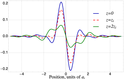
Figure 13: Plots of ${\cal P}_{\varphi}(u,z)$ for different values of $z$. The lateral position is in units of $a_{i}$

The averaged spread functions $\langle P_{\varphi}^{(m)}(x,y,z)\rangle_{y}$ and $\langle P_{\varphi}^{(m)}(x,y,z)\rangle_{x}$ are expressed in terms of the function ${\cal P}(x,z)$

$$\langle P_{\varphi}^{(m)}(x,y,z)\rangle_{y}=\left\{\begin{array}[]{ll}{\cal P}_{\varphi}(x+z,z),&m=1,\\ {\cal P}_{\varphi}(-x+z,z),&m=2,\\ {\cal P}_{\varphi}(-x+z,z),&m=3,\\ {\cal P}_{\varphi}(x+z,z),&m=4,\end{array}\right.$$ (70)

$$\langle P_{\varphi}^{(m)}(x,y,z)\rangle_{x}=\left\{\begin{array}[]{ll}{\cal P}_{\varphi}(y+z,z),&m=1,\\ {\cal P}_{\varphi}(y+z,z),&m=2,\\ {\cal P}_{\varphi}(-y+z,z),&m=3,\\ {\cal P}_{\varphi}(-y+z,z),&m=4,\end{array}\right.$$ (71)

where $\langle..\rangle_{x,y}$ is the average over $x$ or $y$ coordinates, and we defined

$${\cal P}_{\varphi}(u,z)=-\int_{0}^{1}{\rm d}q\,\sin\left(2\pi uq\right)\tilde{g}_{-}(q,z).$$ (72)

The dependence of function ${\cal P}_{\varphi}(u,z)$ on the coordinate $u$ is shown in Fig. 13 for different defocus distances.

Eqs. (62) and (64) can be used to identify $z$. Once the defocus distance $z$ is known, we can separate the effects of blurring and shearing. The latter is accounted for by including the corresponding phase factors in the definitions of the tilt transfer functions:

$$\tilde{P}^{x}_{\theta} = e^{-i2\pi z(k_{x}+k_{y})}\tilde{P}_{\varphi}^{(1)}+e^{-i2\pi z(k_{x}-k_{y})}\tilde{P}_{\varphi}^{(4)}$$

$$-e^{i2\pi z(k_{x}-k_{y})}\tilde{P}_{\varphi}^{(2)}-e^{i2\pi z(k_{x}+k_{y})}\tilde{P}_{\varphi}^{(3)},$$

$$\tilde{P}^{y}_{\theta} = e^{-i2\pi z(k_{x}+k_{y})}\tilde{P}_{\varphi}^{(1)}+e^{i2\pi z(k_{x}-k_{y})}\tilde{P}_{\varphi}^{(2)}$$ (73)

$$-e^{i2\pi z(k_{x}+k_{y})}\tilde{P}_{\varphi}^{(3)}-e^{-i2\pi z(k_{x}-k_{y})}\tilde{P}_{\varphi}^{(4)}.$$

The tilt transfer functions are given by

$$\tilde{P}^{x}_{\theta}({\bf k},z) = 2i\,\tilde{g}_{-}(k_{x},z)\tilde{g}_{+}(k_{y},z),$$

$$\tilde{P}^{y}_{\theta}({\bf k},z) = 2i\,\tilde{g}_{-}(k_{y},z)\tilde{g}_{+}(k_{x},z),$$ (74)

and can be used for phase reconstruction (43) with the resolution defined by the detection aperture, at least for small enough defocus distances.

9.7 Imaging an out-of-focus phase step

A phase step located a distance $z$ away from the focal plane is characterized in frequency space by (33).

For a system with matched illumination and detection apertures, ${\rm NA_{i}}={\rm NA_{d}}$, the intensities detected in the first and second quadrants are obtained using the transfer functions (65):

$$I^{(1)}_{\varphi} = \frac{I_{0}\varphi_{0}}{2\pi}\int_{0}^{1}{\rm d}q\,\frac{\tilde{g}_{-}(q,z)}{q}\cos\left[2\pi q\left(x+z\right)\right],$$

$$I^{(2)}_{\varphi} = -\frac{I_{0}\varphi_{0}}{2\pi}\int_{0}^{1}{\rm d}q\,\frac{\tilde{g}_{-}(q,z)}{q}\cos\left[2\pi q\left(x-z\right)\right].$$ (75)

Fig. 10 illustrates these functions for defocus distances $z=0$, $z=5$ and $z=20$ (in dimensionless units).

9.8 Out-of focus imaging when ${\rm NA_{i}}<{\rm NA_{d}}$

When the numerical apertures of the illumination and detection are not matched, then, according to Eqs. (62) and (64), the pairs of reduced transfer functions are related to one another by the phase factors $e^{i4\pi zk_{x}}$ and $e^{i4\pi zk_{y}}$ only within the tilt bandwidth $|k_{x,y}|\leq 1/2$ (in dimensionless units). The phase factor relating the functions changes for spatial frequencies outside this range. In that case, phase reconstruction of out-of-focus objects remains possible, although with a spatial resolution reduced compared to the case of matched numerical apertures, at least for small enough defocus distance $z$.

The formalism presented in Section 9.6 remains applicable provided the bandwidth of the transfer functions (67), (68) and (9.6) is reduced to the tilt range $|k_{x,y}|\leq 1/2$ (in dimensionless units). The transfer functions can be used for identification of defocus distance and phase reconstruction (43) with the resolution defined by the tilt range for relatively small defocus distances.

References

• [1] G. Popescu, Quantitative phase imaging of cells and tissues, McGraw-Hill Biophotonics, McGraw-Hill (2011).
• [2] F. Zernike, “Das Phasenkontrastverfahren bei der mikroskopischen Beobachtung,” Z. Tech. Phys. 16, 454 (1935).
• [3] G. Popescu, L. P. DeFlores, J. C. Vaughan, K. Badizadegan, H. Iwai, R. R. Dasari, and M. S. Feld, “Fourier phase microscopy for investigation of biological structures and dynamics,” Opt. Lett. 29, 2503-2505 (2004).
• [4] S. Bernet, A. Jesacher, S. Fuerhapter, C. Maurer, and M. Ritsch-Marte,“Quantitative imaging of complex samples by spiral phase contrast microscopy,” Opt. Express 14, 3792-3805 (2006).
• [5] G. Nomarski, “Microinterféromètredifférentiel à ondes polarisées,” J. Phys. Radium 16, S9 (1955).
• [6] M. R. Arnison, K. G. Larkin, C. J. R. Sheppard, N. I. Smith, and C. J. Cogswell, “Linear phase imaging using differential interference contrast microscopy,” J. Microsc. 214, 7-12 (2004).
• [7] M. Shribak, J. LaFountain, D. Biggs, and S. Inoue, “Orientation-independent differential interference contrast microscopy and its combination with an orientation-independent polarization system,” J. Biomed. Opt. 13, 014011 (2008).
• [8] N. Streibl, “Phase imaging by the transport equation of intensity,” Opt. Commun. 49, 6-10 (1984).
• [9] D. Paganin and K. A. Nugent, “Noninterferometric Phase Imaging with Partially Coherent Light ,” Phys. Rev. Lett. 80, 2586-2589 (1998).
• [10] S. S. Kou, L. Waller, G. Barbastathis, and C. J. R. Sheppard, “Transport-of-intensity approach to differential interference contrast (TI-DIC) microscopy for quantitative phase imaging,” Opt. Lett. 35, 447-449 (2010).
• [11] W. C. Stewart, “On differential phase contrast with an extended illumination source,” J. Opt. Soc. Am. 66, 813-818 (1976).
• [12] B. C. Platt and R. Shack, “History and principles of Shack- Hartmann wavefront sensing,” J. Refract. Surg. 17, S573-S577 (2001).
• [13] R. Yi, K. K. Chu, and J. Mertz, “Graded-field microscopy with white light,” Opt. Express 14, 5191-5200 (2006).
• [14] S. B. Mehta and C. J. R. Sheppard, “Quantitative phase-gradient imaging at high resolution with asymmetric illumination-based differential phase contrast,” Opt. Lett. 34, 1924-1926 (2009).
• [15] P. Bon, G. Maucort, B. Wattellier, and S. Monneret, “Quadriwave lateral shearing interferometry for quantitative phase microscopy of living cells,” Opt. Express 17, 13080-13094 (2009).
• [16] I. Iglesias, “Pyramid phase microscopy,” Opt. Lett. 36, 3636 (2011).
• [17] L. Tian, J. Wang, and L. Waller, “3D differential phase-contrast microscopy with computational illumination using an LED array,” Opt. Lett. 39, 1326-1329 (2014).
• [18] A. B. Parthasarathy, K. K. Chu, T. N. Ford, and J. Mertz, “Quantitative phase imaging using a partitioned detection aperture," Opt. Lett. 37, 4062 (2012).
• [19] R. Barankov and J. Mertz, “Single-exposure surface profilometry using partitioned aperture wavefront imaging", Opt. Lett. 38, 3961 (2013).
• [20] J. Li, D. R. Beaulieu, H. Paudel, R. Barankov, T. G. Bifano and J. Mertz, “Conjugate adaptive optics in widefield microscopy with an extended-source wavefront sensor", Optica 2, 682 (2015).
• [21] R. Ng, “Fourier slice photography,” Proc. SIGGRAPH 24, 735-744 (2005).
• [22] M. Levoy, R. Ng, A. Adams, M. Footer, and M. Horowitz, “Light Field Microscopy,” Proc. SIGGRAPH 25, 1-11 (2006).
• [23] X. Xiao, B. Javidi, M. Martinez-Corral, and A. Stern, “Advances in three-dimensional integral imaging: sensing, display, and applications [Invited],” Appl. Opt. 52, 546-560 (2013).
• [24] J. Mertz, Introduction to Optical Microscopy, Roberts and Company Publishers, Greenwood Village, Colorado (2009).
• [25] K. A. Nugent, “The measurement of phase through the propagation of intensity: an introduction,” Contemp. Phys. 52, 55-69 (2011).
• [26] H. Rose, “Nonstandard imaging methods in electron microscopy,” Ultramicroscopy 2, 251-267 (1977).
• [27] D. Hamilton, C. Sheppard, and T. Wilson, “Improved imaging of phase gradients in scanning optical microscopy,” J. Microsc. 135, 275 (1984).
• [28] N. Streibl, “Three-dimensional imaging by a microscope,” J. Opt. Soc. Am. A 2, 121–127 (1985).