Systematics of strength function sum rules

Abstract

Sum rules provide useful insights into transition strength functions and are often expressed as expectation values of an operator. In this letter I demonstrate that non-energy-weighted transition sum rules have strong secular dependences on the energy of the initial state. Such non-trivial systematics have consequences: the simplification suggested by the generalized Brink-Axel hypothesis, for example, does not hold for most cases, though it weakly holds in at least some cases for electric dipole transitions. Furthermore, I show the systematics can be understood through spectral distribution theory, calculated via traces of operators and of products of operators. Seen through this lens, violation of the generalized Brink-Axel hypothesis is unsurprising: one expects sum rules to evolve with excitation energy. Furthermore, to lowest order the slope of the secular evolution can be traced to a component of the Hamiltonian being positive (repulsive) or negative (attractive).

One important way to investigate quantum systems both experimentally and theoretically are through strength functions,

$$S(E_{i},E_{x})=\sum_{f}\delta(E_{x}-E_{f}+E_{i})|\langle f|\hat{\cal O}|i\rangle|^{2}.$$ (1)

which is the probability to transition from a state at initial energy $E_{i}$ to some final state at an energy $E_{f}=E_{i}+E_{x}$, via the operator $\hat{\cal O}$; $|i\rangle$ and $|f\rangle$ are initial and final states, respectively. In particular I consider strength functions sum rules for atomic nuclei for transitions such as electric dipole (E1), magnetic dipole (M1), electric quadrupole (E2), Gamow-Teller (GT), and others [1, 2]. Such transitions not only provide important diagnostics of nuclear structure, and thus test theoretical descriptions of nuclei against experiment, but also have important impacts in astrophysical physical processes such as nucleosynthesis [3, 4, 5, 6, 7], neutrino transport [8], in the experimental extraction of the density of states [9, 10, 12, 11], and so on. These applications include initial states excited far above the ground state.

Often one sees the strength function displaying either a sharp or a broad peak, which is called a resonance, and if most of the strength is in that peak, it is a giant resonance [13]. Giant resonances can have an intuitive picture: for example, for the giant (electric) dipole resonance, or GDR, one envisions protons and neutrons collectively oscillating against each other [14, 15].

The Brink-Axel hypothesis [16, 17] states that if the ground state has a giant electric dipole resonance, then the excited states should have giant dipole resonances as well; because the GDR is explained by a collective proton-versus-neutrons oscillations, it should not be very sensitive to the details of the initial state, and so the strength function $S(E_{i},E_{x})$ in (1) should independent, or nearly so, of $E_{i}$ . While the original Brink-Axel hypothesis only concerned the GDR, it later became a simplifying assumption applied to more general transitions, for example M1 and GT. As strength functions off excited state are particularly difficult to measure experimentally, this hypothesis, if true, would be very useful.

But is the Brink-Axel hypothesis true, especially for transitions other than electric dipole? And if it is not true, can we do anything about it?

Despite wide usage and some early experiments in support of the Brink-Axel hypothesis [18], there is considerable evidence the Brink-Axel hypothesis fails or is modified for E1 [19, 20, 21, 22, 6], M1 [21, 24, 23], E2 [21, 25], and Gamow-Teller [26, 27, 8] transitions. Nonetheless, as stated in a recent Letter [24], “It is quite common to adopt the so-called Brink-Axel hypothesis which states that the strength function does not depend on the excitation energy.” On the other hand, a recent ab initio calculation supported the Brink-Axel hypothesis for E1 transitions from low-lying states [28] and the success and consistency of the Oslo method for determining the level density relies upon M1 strengths following the Brink-Axel hypothesis [9, 10, 11, 12].

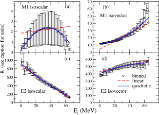
Figure 1: Non-energy weighted sum rules (here denoted as $R$) as a function of initial energy $E_{i}$ for ³³P computed in the $sd$ space. The units for summed M1 strengths (plots (a) and (b)) are $\mu_{N}^{2}$ ($\mu_{N}=$ nuclear magneton), while those for E2 (plots (c) and (d)) are $e^{2}$-fm⁴. The (red) dashed line is the linear approximation to the secular behavior of $R$, derived from spectral distribution theory, while the (blue) solid line is the quadratic approximation.

To simplify the question, I focus on sum rules derived from (1), in particular the total strength or non-energy-weighted sum rule (NEWSR),

$$R(E_{i})=\int S(E_{i},E)dE=\sum_{f}|\langle f|\hat{\cal O}|i\rangle|^{2}$$

$$=\langle i|\hat{\cal O}^{\dagger}\hat{\cal O}|i\rangle=\langle i|\hat{R}|i\rangle,$$ (2)

where for convenience I’ve defined $\hat{\cal O}^{\dagger}\hat{\cal O}=\hat{R}$. If $\hat{\cal O}$ is a non-scalar operator with angular momentum rank $K$ and isospin rank $I$, then $\hat{R}=\sum_{M,\mu}(-1)^{M+\mu}$ $\hat{\cal O}_{K\,-M,I\,-\mu}\hat{\cal O}_{K\,M,I\,\mu}$. (This definition includes a sum over charge-changing transitions for $I=1$, but in return $\hat{R}$ is a simpler, isoscalar operator; I have no reason to believe this qualitatively changes any of my conclusions.) Many other sum rules, such as the energy-weighted sum rule (EWSR), can also be written as expectation values of operators [13], although here I will only consider the NEWSR.

If the Brink-Axel hypothesis were true, then $R(E_{i})$ would be a constant. I investigate the systematics of the non-energy-weighted sum rule for several different operators $\hat{\cal O}$ and nuclides as a function of the initial energy $E_{i}$. To test whether or not $R(E_{i})$ does or does not vary with initial energy $E_{i}$, I first carry out calculations in a detailed microscopic model, the configuration-interaction (CI) shell model. In the CI shell model, one diagonalizes the many-body Hamiltonian in a finite-dimensioned, orthonormal basis of Slater determinants, which are antisymmeterized products of single-particle wavefunctions, typically expressed in an occupation representation [29]. The advantage of CI shell model calculations is that one can generate excited states easily, and for a modest dimensionality one can generate all the eigenstates in the model space.

I use the BIGSTICK CI shell model code [30], which calculates the many-body matrix elements $H_{\alpha\beta}=\langle\alpha|\hat{H}|\beta\rangle$ and then solves $\hat{H}|i\rangle=E_{i}|i\rangle.$ Greek letters ($\alpha,\beta,\ldots$) enote generic basis states, while lowercase Latin letters ($i,j,\ldots$) label eigenstates. As BIGSTICK computes not only the energies but also the wavefunctions, the sum rule $R(E_{i})$ is an expectation value easy to calculate.

For this study I use phenomenological spaces and interactions, although one could also consider ab initio calculations as well; the latter tend to have very large dimensions though, making them less practical for studying the secular behavior over many MeV. Instead I carried out calculations in the $1s_{1/2}$-$0d_{3/2}$-$0d_{5/2}$ or $sd$ shell, using a universal $sd$ interaction version ‘B’ (USDB) [31]. I also consider the following transition operators: M1, E2, and Gamow-Teller using their standard forms [1, 13, 29]. I do not use effective charges, I use harmonic oscillator wavefunctions with an oscillator length of 2.5 fm, I divide sum rules for isovector operators by 3 to roughly average over charge-changing transitions, and use a quenched value of $g_{A}\approx 1$; these assumptions are scaling factors and do not affect my conclusions.

Fig. 1 shows the NEWSR as a function of initial energy (relative to the ground state) for the nuclide ³³P for isoscalar and isovector M1 and E2 transitions, while Fig. 2 shows the NEWSR for Gamow-Teller for several even-even, odd-odd, and odd-$A$ nuclides. (Because I am taking the sum over charge-changing transitions and not the difference, the Ikeda sum rule will not tumble out of these calculations.) I binned the NEWSR into 2 MeV bins, but found the size of the fluctuations shown by errors bars to be insensitive to the size of the bins. Other calculations not shown show qualitatively similar results, which can be summarized as:

$\bullet$ Both the secular (average) behavior of the NEWSR and fluctuations thereof show surprisingly smooth behavior.

$\bullet$ As illustrated for Gamow-Teller transitions in Fig. 2 (and duplicated but not shown for other operators), the behavior is relatively insensitive to the nuclide.

$\bullet$ Nonetheless, the behavior does depend sharply upon the transition: isoscalar E2 falls sharply with initial energy, isovector M1 and Gamow-Teller grow, and isoscalar M1 has large fluctuations.

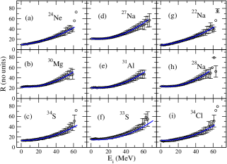
Figure 2: Non-energy weighted Gamow-Teller sum rules (here denoted as $R$) as a function of initial energy $E_{i}$ for several nuclides in the $sd$ space. The (blue) solid line is the quadratic approximation to the secular behavior of $R$, derived from spectral distribution theory.

As the Brink-Axel hypothesis predicts NEWSR independent of $E_{i}$, these results numerically confirm the previously mentioned experimental and theoretical evidence against Brink-Axel. Given the simple yet non-trivial systematics, can one understand these results from basic principles?

If one is computing $R(E_{i})$ in a finite model space, such as the CI shell model, and that model space has dimension $N$, then one can compute the average sum rule, that is, the average expectation value,

$$\frac{1}{N}\sum_{i=1}^{N}\langle i|\hat{\cal O}^{\dagger}\hat{\cal O}|i\rangle=\frac{1}{N}\sum_{i}\langle i|\hat{R}|i\rangle\equiv\overline{\langle\hat{R}\rangle},$$ (3)

If we compute the matrix elements of $\hat{R}$ in some orthonormal many-body basis, for example Slater determinants in the framework of the CI shell model, the sum is just a trace of the matrix. Because a trace is invariant under a unitary transformation, we can sum over any convenient set of basis states $\{|\alpha\rangle\}$. This invariance under the trace is important because the trace can be used as an inner product in the space of Hermitian operators in the framework of spectral distribution theory (SDT), also sometimes called statistical spectroscopy [32, 33, 34, 35, 36, 37, 38].

[The notation $\langle\hat{R}\rangle=\langle i|\hat{R}|i\rangle$ signifies the expectation value being an average over many measurements for the same state. Yet for SDT one averages the expectation value over all states in a space, usually defined by fixed quantum numbers such as the number of particles. Practitioners of SDT frequently use the notation $\langle\hat{A}\rangle^{(m)}$ for (3) [36, 37, 38], where $m$ denotes the number of particles and possibly other quantum numbers, and the trace is implied to be restricted to states with those quantum numbers. Because of the unfortunate possibility of confusion with the expectation value proper, I introduced a hybrid notation $\overline{\langle\hat{R}\rangle}$ for the average (3).]

To see if the sum rule $R(E_{i})$ does indeed have a secular dependence upon the initial energy $E_{i}$, one can take a weighted average, namely,

$$\frac{1}{N}\sum_{i}R(E_{i})E_{i}=\frac{1}{N}\sum_{i}\langle i|\hat{R}\hat{H}|i\rangle=\overline{\langle\hat{R}\hat{H}\rangle}.$$ (4)

Again, since this is a trace, one can compute in any convenient basis. French proposed [33] the following inner product between two Hamiltonians, or more broadly between two Hamiltonian-like (Hermitian and angular momentum scalar) operators:

$$\left(\hat{H}_{1},\hat{H}_{2}\right)=\overline{\left\langle\left(\hat{H}_{1}-\overline{\langle\hat{H}_{1}}\rangle\right)\left(\hat{H}_{2}-\overline{\langle\hat{H}_{2}\rangle}\right)\right\rangle}$$

$$=\overline{\langle\hat{H}_{1}\hat{H}_{2}\rangle}-\overline{\langle\hat{H}_{1}\rangle}\,\,\,\overline{\langle\hat{H}_{2}\rangle}.$$ (5)

The appeal of this definition of the inner product between Hamiltonian-like operators is that, if the operators are angular momentum scalars and if one works in a finite, spherically symmetric shell-model single-particle space, one can calculate the traces directly without constructing the matrix [32, 36, 37, 38]. One can sum over states with specified isospin (while one can take sums over specified angular momentum [39], the resulting formulas are significantly more tedious and computationally intensive) or even just on subspaces defined by configurations, that is, a fixed number of particles in each orbit. In principle one can take higher-order moments or work with Hamiltonians or particle rank higher than two. For this work, however, I use a recent code [38] which reads in only isospin-invariant two-body interactions and which calculates at most second moments (i.e., the inner product defined above) working in spaces with fixed total number of valence particles $A_{\mathrm{val}}$ and total isospin $T$.

With the definition of an inner product in the space of operators, we can return to the question of the invariance of the strength function with initial energy. One necessary, but by no means sufficient, condition for the invariance of the strength function is that the total strength not change with initial energy, that is, $R(E_{i})\approx$ constant. Such a condition implies $\overline{\langle\hat{R}\hat{H}\rangle}\approx\overline{\langle\hat{R}\rangle}\,\,\,\overline{\langle\hat{H}\rangle},$ but this reduces to the inner product $(\hat{R},\hat{H})=\overline{\langle\hat{R}\hat{H}\rangle}-\overline{\langle\hat{R}\rangle}\,\,\overline{\langle\hat{H}\rangle}\approx 0$, that is, the Hamiltonian $\hat{H}$ and the operator $\hat{R}$ must be “orthogonal” in a well-defined way. While this could happen by accident, in general it will not, as we already see in the examples above.

As it turns out, the above condition corresponds to the linear dependence of $R(E_{i})$ on $E_{i}$. We can go to a higher order polynomial description, especially if we assume that the state density of the many-body Hamiltonian is well-described by a Gaussian with centroid $\bar{E}$ and width $\sigma$, that is,

$$\rho(E)=N(2\pi\sigma^{2})^{-1/2}\exp\left(-\frac{(E-\bar{E})^{2}}{2\sigma^{2}}\right),$$ (6)

which is often a good assumption for nuclei [35]. In the language of spectral distribution theory,

$$\bar{E}=\overline{\langle\hat{H}\rangle},$$ (7)

$$\sigma^{2}=\overline{\langle\hat{H}^{2}\rangle}-\left(\overline{H}\right)^{2}.$$ (8)

Let’s further assume that the sum rule $R(E)$ is a quadratic polynomial in $E$:

$$R(E)=R_{0}+R_{1}\frac{(E-\bar{E})}{\sigma}+R_{2}\frac{(E-\bar{E})^{2}}{\sigma^{2}}.$$ (9)

Then one can easily compute the following averages:

$$\overline{R}=\overline{\langle\hat{R}\rangle}=R_{0}+R_{2};$$ (10)

$$(\hat{R},\hat{H})/\sigma=R_{1}.$$ (11)

One could add an additional constraint by by higher moments, for example $\overline{\langle\hat{R}\hat{H}^{2}\rangle}$. While such higher moments are calculable [37], the formula are cumbersome and prone to slow evaluation; furthermore experience in unpublished work suggests even higher moments have difficulty in describing the tails of distributions [40]. (This is understandable; the traces are just averages, after all, and dominated by the density of states in the middle of the spectrum.) Instead, I use the sum rule at the ground state energy $E_{gs}$, which is often accessible:

$$R(E_{gs})=R_{0}+R_{1}\frac{(E_{gs}-\bar{E})}{\sigma}+R_{2}\frac{(E_{gs}-\bar{E})^{2}}{\sigma^{2}}.$$ (12)

These equations (10,11,12) can be easily solved.

Fig 1 shows both linear (red dashed lines) and quadratic (blue solid lines) approximations to $R(E_{i})$. Although the linear approximation demonstrates a secular dependence on $E_{i}$, in general the quadratic does better in describing the secular evolution of the sum rule. Fig. 2 shows only the quadratic approximation.

Now, as illustrated in the figures, while one has smooth secular behavior, there are nontrivial fluctuations about the secular trends. The fluctuations are insensitive to the size of the energy bins. Although the fluctuations about the smooth secular behavior are not easily written in terms of traces, one might be able to derive the fluctuations from random matrix theory; but this will have to be left to future work.

The original Brink-Axel hypothesis described E1 strength functions. To explore them, I use a space with opposite parity orbits, the $0p_{1/2}$-$0p_{3/2}$-$1s_{1/2}$-$0d_{5/2}$ or $p$-$sd_{5/2}$ space, chosen so I could fully diagonalize for some nontrivial cases. For an interaction I use the Cohen-Kurath (CK) matrix elements in the $0p$ shell[41], the older USD interaction [42] in the $0d_{5/2}$-$1s_{1/2}$ space, and the Millener-Kurath (MK) $p$-$sd$ cross-shell matrix elements[43]. Within the $p$ and $sd$ spaces I use the original spacing of the single-particle energies for the CK and USD interactions, respectively, but then shift the $sd$ single-particle energies up or down relative to the $p$-shell single particle energies to get the first $3^{-}$ state at approximately $6.1$ MeV above the ground state. The rest of the spectrum, in particular the first excited $0^{+}$ state, is not very good, but the idea is to have a non-trivial model, not exact reproduction of the spectrum. Because this space does not allow for exact center-of-mass projection I restrict myself to isovector E1 transitions. The resulting NEWSRs are shown in Fig. 3, illustrating only a weak violation of Brink-Axel.

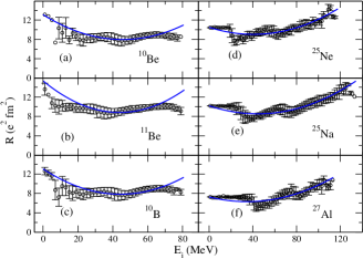
Figure 3: Non-energy weighted isovector E1 sum rules (here denoted as $R$) as a function of initial energy $E_{i}$ for several nuclides in the $p$-$sd_{5/2}$ space. The (blue) solid line is the quadratic approximation to the secular behavior of $R$, derived from spectral distribution theory.

Although the quadratic approximation captures the general trends, the secular behavior for $R(E)$ is not as smooth. This may be because of the model space. The density of states for these nuclides, for example, are not as Gaussian-like as for the $sd$-shell examples shown; the beryllium and boron nuclides have large third moments, while the the neon, sodium, and aluminum nuclides have larger fourth moments (“fat tails”) than Gaussians.

Nonetheless, not only do we have evidence that the generalized Brink-Axel hypothesis is not followed, we can understand why. Previous work has suggested specific reasons for breaking the Brink-Axel hypothesis: changes in deformation as one goes up in energy explains the increase in width for the GDR [20], while a decrease in spatial symmetry/increase in SU(4) symmetry explains the increase of strength in Gamow-Teller sum rules [26]. Spectral distribution theory provides a more general understanding. By establishing a vector space for Hamiltonians such that

$$\hat{H}=\sum_{\sigma}c_{\sigma}\hat{R}_{\sigma},$$ (13)

the inner product defined by SDT yields $(\hat{H},\hat{R}_{\sigma})=c_{\sigma}$ (up to some easily-defined normalization). Here is the key point: if $c_{\sigma}<0$, that is, attractive, one expects a negative slope to $R(E)$ and more strength for low-lying initial states. This is seen in Fig (1)(c),where the operator $\hat{R}\sim Q\cdot Q$, the quadrupole-quadrupole interaction. If, on the other hand, $c_{\sigma}>0$, that is repulsive, as for $(\sigma\tau)^{2}$ as in Fig. (2), low-lying states have less total strength. Only if $c_{\sigma}\approx 0$ could the Brink-Axel hypothesis be true, at least at the lowest level. Of course, the linear approximation is not always sufficient to fully describe the secular behavior; for many cases one needs at least quadratic and possibly even higher-order terms [40].

In summary, I have numerically demonstrated that that the non-energy weighted sum rule for transition operators applied to several sample nuclides evolves with the energy of the initial state–weakly for the case of isovector E1, and more strongly for other operators–and furthermore that such variation is expected from spectral distribution theory. In particular, one can predict qualitatively whether a sum rule will grow or shrink in magnitude with initial energy, depending if part of the Hamiltonian (that part proportional to the operator $\hat{R}$ for the sum rule, that is, the square of the transition operator for the NEWSR) is attractive or repulsive. In many cases one needs higher moments for accurate quantitative predictions , but it should be clear now that one should only invoke Brink-Axel with caution.

This material is based upon work supported by the U.S. Department of Energy, Office of Science, Office of Nuclear Physics, under Award Number DE-FG02-96ER40985.

References

- [1] A. Bohr and B. R. Mottelson, Nuclear structure, (World Scientific, Singapore, 1998).
- [2] R. D. Lawson, Theory of the nuclear shell model, (Clarendon Press, Oxford, 1980).
- [3] G. M. Fuller, W. A. Fowler, and M. J. Newman, Astrophys. J. (Supplement) 42 (1980) 447.
- [4] G. M. Fuller and B. S. Meyer, Astrophys. J. (Supplement) 453 (1995) 792.
- [5] A. C. Larsen and S. Goriely, Phys. Rev. C 82 (2010) 014318.
- [6] E. Litvinova and N. Belov Phys. Rev. C 88 (2013) 031302(R).
- [7] N. Tsoneva, S. Goriely, H. Lenske, and R. Schwengner Phys. Rev. C 91 (2015) 044318.
- [8] G. W. Misch, G. M. Fuller, and B. A. Brown, Phys. Rev. C 90 (2014) 065808.
- [9] A. Schiller, L. Bergholt, M. Guttormsen, E. Melby, et al. Nucl. Instrum. Methods Phys. Res. A 447 (2000) 498.
- [10] A. Schiller, E. Algin, L. A. Bernstein, P. E. Garrett, et al., Phys. Rev. C 68 (2003) 054326.
- [11] N. U. H. Syed, M. Guttormsen, F. Ingebretsen, A. C. Larsen, et al., Phys. Rev. C 79 (2009) 024316.
- [12] A. V. Voinov, S. M. Grimes, U. Agvaanluvsan, E. Algin, et al., Phys. Rev. C 74 (2006) 014314.
- [13] P. Ring and P. Shuck, The nuclear many-body problem (Springer-Verlag, New York 1980).
- [14] M. Goldhaber and E. Teller, Phys. Rev. 74 (1948) 1046.
- [15] H. Steinwedel and J. H. D. Jensen, Z. Naturforsch. A5 (1950) 413.
- [16] D. Brink, D. Phil. thesis, Oxford University (unpublished), 1955.
- [17] P. Axel, Phys. Rev. 126 (1962) 671.
- [18] S. Raman, O. Shahal, and G. G. Slaughter, Phys. Rev. C 23 (1981) 2794.
- [19] J. Ritman, F.-D. Berg, W. Kühn, V. Metag, et al, Phys. Rev. Lett. 70 (1993) 533.
- [20] A. Bracco, F. Camera, M. Mattiuzzi, B. Million, et al., Phys. Rev. Lett. 74 (1995) 3748.
- [21] A. C. Larsen, M. Guttormsen, R. Chankova, F. Ingebretsen, et al., Phys. Rev. C 76 (2007) 044303.
- [22] C. T. Angell, S. L. Hammond, H. J. Karwowski, J. H. Kelley, et al., Phys. Rev. C. 86 (2012) 051302(R).
- [23] B. Alex Brown and A. C. Larsen, Phys. Rev. Lett. 113 (2014) 252502.
- [24] R. Schwengner, S. Frauendorf, and A. C. Larsen, Phys. Rev. Lett. 111 (2013) 232504 .
- [25] R. Schwengner, Phys. Rev. C 90 (2014) 064321.
- [26] N. Frazier, B. A. Brown, D. J. Millener, and V. Zelevinsky, Phys. Lett. B 414(1997) 7.
- [27] J.-U. Nabi and M. Sajjad, Phys. Rev. C 76 (2007) 055803.
- [28] M. K. G. Kruse, W. E. Ormand, and C. W. Johnson, arXiv:1502.03464
- [29] P.J. Brussard and P.W.M. Glaudemans, Shell-model applications in nuclear spectroscopy (North-Holland Publishing Company, Amsterdam 1977).
- [30] C. W. Johnson. W. E. Ormand, and P. G. Krastev, Comp. Phys. Comm. 182 (2013) 2235.
- [31] B.A. Brown and W.A. Richter, Phys. Rev. C 74 (2006) 034315.
- [32] H. Bannerjee and J. B. French, Phys. Lett. 23 (1966) 245; J. B. French, Phys. Lett. 23 (1966) 248.
- [33] J. B. French, Phys. Lett. B 26 (1967) 75.
- [34] J.B. French and K.F. Ratcliff, Phys. Rev. C 3 (1971) 94.
- [35] K. K. Mon and J. B. French, Ann. Phys. 95 (1975) 90.
- [36] J. B. French and V. K. B. Kota, Phys. Rev. Lett. 51 (1983) 2193; V. K. B. Kota, V. Potbhare and P. Shenoy, Phys. Rev. C 34 (1986) 2330.
- [37] S. S. M. Wong, Nuclear Statistical Spectroscopy, Oxford Press (New York, 1986).
- [38] K.D. Launey, S. Sarbadhicary, T. Dytrych, J.P. Draayer Comp. Phys. Comm. 185 (2014) 254.
- [39] R. A. Sen’kov, M. Horoi. and V. G. Zelevinksy, Comp. Phys. Comm. 184 (2013) 215.
- [40] C. W. Johnson, J. Nabi, and W. E. Ormand, arXiv:nucl-th/0111068.
- [41] S. Cohen and D. Kurath, Nucl. Phys. 73 (1965) 1.
- [42] B.H. Wildenthal, Prog. Part. Nucl. Phys. 11 (1984) 5 .
- [43] D. J. Millener and D. Kurath, Nucl. Phys A 255 (1975) 315 .