A Definition for Giant Planets Based on the
Mass $-$ Density Relationship

Abstract

We present the mass-density relationship (log $M$ - log $\rho$) for objects with masses ranging from planets ($M$ $\approx$ 0.01 $M_{Jup}$) through stars ($M$ $>$ 0.08 $M_{\odot}$). This relationship shows three distinct regions separated by a change in slope in log $M$ – log $\rho$ plane. In particular, objects with masses in the range 0.3 $M_{Jup}$ to 60 $M_{Jup}$ follow a tight linear relationship with no distinguishing feature to separate the low mass end (giant planets) from the high mass end (brown dwarfs). The distinction between giant planets and brown dwarfs thus seems arbitrary. We propose a new definition of giant planets based simply on changes in the slope of the log $M$ versus log $\rho$ relationship. By this criterion, objects with masses less than $\approx$ 0.3 $M_{Jup}$ are low mass planets, either icy or rocky. Giant planets cover the mass range 0.3 $M_{Jup}$ to 60 $M_{Jup}$. Analogous to the stellar main sequence, objects on the upper end of the giant planet sequence (brown dwarfs) can simply be referred to as “high mass giant planets”, while planets with masses near that of Jupiter can be considered to be “low mass giant planets”.

1 Introduction

The nature of stellar and sub-stellar objects is determined by their mass. Stars are defined as an object with sufficient mass to ignite hydrogen fusion in the core. Sub-stellar objects, on the other hand, have masses below that needed to ignite hydrogen burning in their cores ($M$ $\sim$ 80 $M_{Jup}$). Like their stellar counterparts, sub-stellar objects encompass a wide range of masses from those that are accepted as planets, with masses of a few $M_{Jup}$, to objects often considered to be brown dwarfs with masses of a few tens of $M_{Jup}$. The exact boundary in mass between what one considers a “planet” and what one considers a “brown dwarf”” is blurred and is still the subject of debate.

One definition of giant planet is that it is a sub-stellar object that has not undergone deuterium burning anytime during its life. By this criterion the boundary between planets and brown dwarfs should be about 13 $M_{Jup}$ (Burrows et al. 2001). However, this distinction seems arbitrary as the mass distribution for companions below 25 $M_{Jup}$ show no characteristic features at this mass limit (Udry 2010). Furthermore, the period of deuterium burning has little influence on the future evolution of the brown dwarf. This is contrary to stars where hydrogen burning under hydrostatic equilibrium significantly alters the further evolution of the object. Chabrier et al. (2014) argued that deuterium burning, or lack thereof, plays no role in either giant planet or brown dwarf formation. They also pointed out that these two types of objects “might bear some imprints of their formation mechanism, notably in their mean density and in the physical properties of their atmosphere.”

On the other hand, the intersection of the mass distributions of sub-stellar objects appear to have a distinctive dip around $M$ $\approx$ 25-30 $M_{Jup}$ (Udry 2010). Schneider et al. (2011) attributed this dip as the boundary between the mass spectrum of planets, which is decreasing with increasing mass, and the distribution of sub-stellar and low mass stars which is increasing beyond this point. The dip is also coincident with a possible break in the mass-radius relationship for low mass and sub-stellar objects (Pont et al. 2005; Anderson et al. 2011) which suggests a difference in the physical natures between objects on either side of this boundary (Schneider et al. 2011). For these reasons Schneider et al. (2011) arbitrarily (our emphasis) assigned a maximum mass of 25 $M_{Jup}$ as the limit for including objects in the Exoplanet Encyclopaedia (www.exoplanet.eu). However, if an object lies near this 25 $M_{Jup}$ boundary we still do not know its nature, i.e. to which distribution (planets or brown dwarfs) it actually belongs.

The mean density versus mass relationship for planets show a broad minimum around a mass of 0.3 $M_{Jup}$ (Rauer et al. 2014; Laughlin & Lissauer 2015) which separates the H/He dominated giant planets from low-mass planets of Neptune-mass or smaller. The different slopes in the density-mass plane of the two objects highlights the differences in structure between the two classes of planets. We extend the density-mass relationship through sub-stellar and stellar objects and show that this also shows a change in slope marking the differences in structure between giant planets/brown dwarfs and stellar objects. We argue for a definition of giant planets based on the mass-density diagram.

2 The Density versus Mass Relationship

We constructed a mass-density diagram for the full range of masses covering planets through main sequence stars. Because all of these are transiting/eclipsing systems these are relatively close pairs. In this sense they can be treated as a “pseudo-homogenous” sample. For the giant planet data we largely restricted our sample to transiting planets from the space based missions CoRoT and Kepler. These space missions provide light curves with the best photometric precision that produce the most accurate planet radii. This is particularly important since the radius enters as the third power in the density. Besides using space-based transit discoveries that provide the best photometric precision, it is important to use transit light curve analyses that were done in a consistent manner. Various investigators may use different limb-darkening laws or apply different methods to filter out intrinsic stellar variability which may introduce more scatter in the results. For this reason we took radius and mass values for the planets from the web-based TEPCat catalog (http://www.astro.keele.ac.uk/jkt/tepcat/tepcat.html
and references therein) as these were derived from a uniform analysis (see Southworth 2010,2011,2013).

There are few mass and radius measurements for brown dwarfs or “super planets” mostly because of the paucity of such objects, so we had to include ground-based results. Along with the Kepler discoveries (Diaz et al. 2013; Diaz et al. 2014; Bouchy et al. 2011; Moutou et al. 2013) we therefore included ground-based results (Johns-Krull et al. 2008; Hellier et al. 2009; Joshi et al. 2009; Siverd et al. 2012; Anderson et al. 2011; Triaud et al. 2013).

Stellar masses and radii for most main sequence stars were taken from Torres, Andersen, & Giménez (2010). A variety of sources were used for the parameters of stars from the low-mass end of the main sequence (Pont et al. 2005, 2006, 2008; Demory et al. 2009; Tal-Or et al. 2013, Ofir et al. 2012; Zhou et al. 2014).

Figure 1 shows the resulting mass-density relationship for our sample. There are two major inflections in the curve. The maximum density occurs at a mass of $\approx$ 60–70 $M_{Jupiter}$, the boundary between core nuclear burning stars and degenerate core brown dwarfs. The second inflection is a minimum in density at $M$ $\approx$ 0.3 $M_{Jupiter}$, roughly the boundary between H/He dominated planets and low mass planets.

Fits were made to the data in these regions in order to define better the boundary between lower mass planets, giant planets/brown dwarfs and stars. Although the stars show a roughly linear relationship, in the mass range 0.08 – 1 $M_{\odot}$ the relationship is best fit by a second order polynomial shown by the curved line. For low mass stars in the range 0.08 – 1 $M_{\odot}$ the log $M$ $-$ log $\rho$ relationship can also be fit by a line resulting in $\rho$ $\propto$ $M^{-(2.09\pm 0.16})$. This follows from the mass-radius relationship on the low mass end of the main sequence where $R$ $\propto$ $M$, thus $\rho$ $\propto$ $M^{-2}$.

The log $M$ – log $\rho$ relationship for giant planets and brown dwarfs show a very tight correlation (correlation coefficient, $r$ = 0.976). A linear fit over the mass range 0.35 – 65 $M_{Jup}$ results in:

$$log\rho=(1.15\pm 0.03)logM-(0.11\pm 0.03)$$

This linear relationship of density with mass simply reflects the fact that objects with masses ranging from giant planets ($\sim$ 1 $M_{Jup}$) up to low mass stars all have approximately the same radius. Thus an increase in mass is accompanied by proportional increase in density. Note that this curve closely follows the mass-density relationship for H/He dominated giant planets (Fortney et al. 2007) which is shown as the dashed line. At the low mass end of the giant planet range, the linear fit to the giant planets deviates significantly from the dashed line for planets with Jupiter-like composition. The planets below the dashed line are larger than expected by such models and called “inflated” planets. The linear relationship intercepts the main sequence for stars at $M$ = 63 $\pm$ 6 $M_{Jup}$.

For simplicity we shall refer to all exoplanets with masses less than $\approx$ 0.3 $M_{Jup}$ as low mass exoplanets. These can be either rocky or ones that have a large fraction of volatiles (i.e. Neptune-like). The low mass planets show considerable scatter in their densities. In spite of this scatter there clearly appears to be a minimum in density around $\sim$ 0.3 $M_{Jup}$. Indeed, a parabolic fit to the valley of this ‘V’-shape results in a minimum of the density at this value for the mass. For higher mass objects the density increases. We take this as the boundary between the low mass planets and giant planets.

Fig. 2 shows the more traditional Mass-Radius relationship with our boundaries shown as the vertical dashed lines. One can also see inflections in this curve at roughly the same boundaries seen in Fig. 1, although these are not as striking or well defined particularly between the low mass and giant planets.

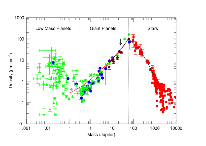
Figure 1: The density and mass of stars (red squares), giant planets and brown dwarfs, and low mass planets. Triangles represent Kepler discoveries and dots are CoRoT exoplanets. Ground-based discoveries for high mass giant planets are shown by pentagons. The line represents a linear fit to the giant planets and brown dwarfs in the mass range $M$ = 0.35 - 60 $M_{Jup}$. A second order polynomial fit (curved line) was made to the lower end of the stellar main sequence. The boundary between the low mass planets and giant planet occurs at $M$ $=$ 0.3 $M_{Jup}$. The boundary between the giant planets and stars is at $M$ $=$ 60 $M_{Jup}$ (0.060 $M_{\odot}$). The dashed red line shows the mass-density relationship for H/He dominated giant planets taken from Fortney et al. (2007).

Figure 2: The points from Figure 1 shown in the mass-radius plane.

3 Discussion

The mass density diagram for all objects with masses ranging from planets to stars are separated by three distinct regions marked by an abrupt change in sign of the slope of the $\log$ M $-$ $\log\rho$ relationship. Stars show a negative slope, whereas giant planets and brown dwarfs have a positive slope. However, below about 0.3 $M_{Jup}$ objects show considerable scatter in their densities. We shall simply refer to this region of the diagram as the “low mass planets” (LMP). It is beyond the scope of this paper to discuss this region of the diagram, the origin of such scatter, or any relationship between the mass and density. Instead we will focus on the giant planets and for the sake of discussion we shall refer to these regions between the LMP and stars as the “gaseous planet sequence” (GPS). MS will refer to the classic main sequence for stars.

The beginning of the GPS occurs at $M$ $\approx$ 0.3 $M_{Jup}$, roughly the boundary between planets with a significant amount of volatiles, and those dominated by H/He. The boundary between the GPS and the MS occurs at 60 $M_{Jup}$. Laughlin & Lissauer (2015) noted that the distribution of planetary densities had a broad minimum at a planet mass of $M_{P}$ $\sim$ 0.1 $M_{J}$ (30 $M_{Earth}$) which they took as the boundary between giant planets and low mass planets (termed “ungiants” in their paper) We propose that this boundary is actually at a much higher mass of $M_{P}$ $\sim$ 0.3 $M_{J}$.

We also fit the density-mass data from Laughlin & Lissauer (2015, Fig. 5 of their paper) for planets with in the mass range 0.01 to 0.1 $M_{J}$. The data are well fit by a linear function that intercepts our GPS at $M_{P}$ $\sim$ 0.3 $M_{J}$ ($\approx$ 100 $M_{Earth}$), consistent with our proposed boundary.

The striking feature about GPS is that there is no distinguishing characteristic that separates the low mass end where objects are clearly planets, and the high mass end where objects are generally considered to be brown dwarfs. The 25 $M_{Jup}$ limit (the arrow in Fig. 1) taken by Schneider et al. (2009) to be the boundary between planets and brown dwarfs shows no obvious differences in the GPS on either side of this limit. If anything, the arrow only seems to mark the boundary where the data are sparce. Clearly, the discovery of more objects in this mass range is desperately needed. Possibly differences between the giant planets and the “traditional” brown dwarfs may become more apparent with more discoveries. For instance, if no objects can be found that fill the gap marked by 25 $M_{Jup}$ (arrow) and the onset of the MS then this “gap” might be taken to separate the planets from the brown dwarfs and stars. For now we note that the few brown dwarfs with masses $\approx$ 60 $M_{Jup}$ all fall on the GPS.

In light of Figure 1 making a distinction between objects on the low- and high-mass end of the GPS seems arbitrary and may only obscure the fact that all objects on this track are physically the same objects governed by the same underlying physics and with similar structure, analogous to the MS. Chabrier et al. (2014) also argued that the mass boundary between giant planets and brown dwarfs given by the present IAU definition was “incorrect and confusing and should be abandoned”. Figure 1 certainly supports this claim. This figure also shows that the density provides us with no obvious hints regarding a different formation mechanism between brown dwarfs and giant planets. Possibly the differences in the physical properties of the atmospheres may show indications of a different formation mechanism (Chabrier et al. 2014).

Comparing the properties of the GPS to the MS provides us with additional arguments to support the claim that all objects along the GPS should be considered the same type of objects. Stars have masses that cover over two orders of magnitude. The structure of the star changes considerably along the main sequence. High mass stars have a convective core and radiative envelope and as one moves down the main sequence this structure changes to objects with a radiative core and a convective envelope. The lowest mass stars, on the other hand, are fully convective. The stellar atmosphere changes considerably along the main sequence in terms of effective temperatures and the types of spectral features that are observed.

Finally, stars may also have different formation scenarios. Low mass stars are believed to form from the collapse of a proto-cloud and subsequent accretion (Palla & Stahler 1993). The formation mechanism for high mass stars is still open to debate. For massive stars radiation from the core halts the accretion process thus limiting the mass (e.g. Yorke & Krügel 1977). One hypothesis is that they are formed by the merger of lower mass stars (Bonnell et al. 1998). Regardless of all these substantial differences, all objects along the MS are considered to be the same general class of objects that is governed by the same physics - nuclear burning in the core under hydrostatic equilibrium. We only make sub-distinctions in the form of “low mass” and “high mass” stars.

Objects along the GPS also have masses that differ by over two orders of magnitudes. Like stars, they certainly have a wide range of effective temperatures, atmospheric features, and possibly even different formation mechanisms. Making an arbitrary distinction between giant planets and brown dwarfs only confuses the central issue that these objects share a similar structure. Analogous to stars we can make subtle distinctions between “high mass giant planets” and “low mass giant plants”, but the class should be considered as a whole in order to gain a more fundamental understanding of their formation, evolution, and nature.

Comparing the GPS to the MS also provides a natural explanation to the so-called “Brown Dwarf Desert”. The paucity of brown dwarf companions simply reflect the decrease in number of high mass much in the same way there is a decrease in the number of high mass stars in the stellar distribution. Compared to low mass main sequence stars O-type stars in our galaxy are extremely rare – it is simply harder for nature to form these higher mass stars. To our knowledge, astronomers never refer to the “O-star desert.”

We propose a new definition of planets, brown dwarfs, and stars based not on arbitrary separation of distributions, or whether short-lived deuterium burning has occurred, or just because we are biased in thinking that giant planets should all have masses close to that of our Jupiter. Rather, our definition is based on the observed inflections in the mass-density diagram that separate regions governed by different underlying physics. Thus,

$M$ $<$ 0.3 $M_{Jup}$ $\Rightarrow$ Low Mass Planets

0.3 $M_{Jup}$ $<$ $M$ $<$ 60 $M_{Jup}$ $\Rightarrow$ Giant Gaseous Planets

$M$ $>$ 60 $M_{Jup}$ $\Rightarrow$ Stellar Objects

We note that by our definition Saturn has a mass near the boundary between low mass planets and gas giant planets. Although we refer to objects with $M$ $>$ 60 $M_{Jup}$ as “stars”, the exact boundary between objects supported by electron degeneracy pressure and those with a hydrogen burning core is not well known and can be as high as 80 $M_{Jup}$. Possibly objects with 60 $M_{Jup}$ $<$ $M$ $<$ 80 $M_{Jup}$ should be considered to be the bona fide brown dwarfs.

Another obvious feature of Figure 1 is the relative paucity of objects in the mass range 20 $<$ $M_{Jup}$ $<$ 100. This is in part due to the relative low number of these with respect to lower mass planets, but may also be due to the fact that Doppler surveys have largely concentrated on confirming transit discoveries of lower mass planets. Low mass stars, and objects on the high mass end of the GPS are often ignored in favor of getting mass measurements on the more “interesting” planet candidates. However, accurate mass and radius measurements of objects on the low mass end of the stellar main sequence and the upper end of the GPS, i.e. the boundary between high mass giant planets and low mass stars, are also important. Only by studying the full range of objects from high mass giant planets to the lower end of the main sequence will we obtain a more fundamental understanding of the formation of giant planets compared to low mass stars.

In much the way the Hertzsprung-Russel Diagram has served as a tool for understanding stellar structure, the M-$\rho$ diagram can serve as a powerful tool for understanding planetary structure.

References

- Anderson et al. (2011) Anderson,D.R., Collier Cameron, A., Hellier, C. et al. 2011, ApJL, 726, 19
- Bonnell et al. (1998) Bonnell, I., Bate. M.R., Zinnecker, H. 1998, MNRAS, 298, 93
- Bouchy et al. (2011) Bouchy, F., Bonomo, A.S., Santerne, A. et al. 2011, A&A, 533, 83
- Burrows et al. (2001) Burrows, A., Hubbard, W.B., Lunine, J.I., Liebert, J. 2001, Rev. Mod. Phys., 73, 719
- Diaz et al. 2013 (2013) Diaz, R. et al. 2013, A&A, 551, 9
- Diaz et al. 2014 (2014) Diaz, R. et al. 2014, A&A, 572, 109
- Fortney et al. 2007 (2007) Fortney, J.J., Marley, M.S., Barnes, J.W. 2007, ApJ, 659. 1661
- Gillon et al. 2012 (2012) Gillon, M., Demory, B.-O., Benneke, B. et al. A&A, 539, 28
- Hellier et al. (2009) Hellier, C., Anderson, D.R., Collier Cameron, A., et al. 2009, Nature, 460, 1098
- Johns-Krull et al. (2008) Johns-Krull, C.M., McCullough, P.R., Burke, C.J. et al. 2008, ApJ, 677, 657
- Joshi et al. (2009) Joshi, Y.C., Pollaco, D., Collier Cameron, A. et al. 2009, MNRAS, 392, 1532
- Laughlin & Lissauer 2015 (2015) Laughlin, G., Lissauer, J.J. 2015, in Treatise on Geohysics (eprint arXiv:1501.05685)
- Moutou et al. (2013) Moutou, C. et al. 2013, A&A, 558, 6
- Ofir et al. (2012) Ofir, A., Gandolfi, D., Buchave, L. et al. 2012, MNRAS, 423, L1
- Pont et al. (2006) Pont, F., Moutou, C., Bouchy, F. et al. 2006, A&A, 447, 1035
- Pont et al. (2008) Pont, F., Tamuz, O., Udalski, A, et al. 2008, A&A, 487, 749
- Rauer et al. (2014) Rauer, H. Catala, C., Aerts, C. et al. 2014, Experimental Astronomy, 38, Issue 1-2, 249
- Schneider et al. (2011) Schneider. J., Dedieu, C., Le Sidaner, P., Savalle, R., Zolotukhin, I. 2011, A&A, 532, 795
- Siverd et al. (2012) Siverd, R.J., Beatty, T.G., Pepper, J. et al. 2012, ApJ, 761, 123
- Southworth (2010) Southworth, J. 2010, MNRAS, 408, 1689
- Southworth (2011) Southworth, J. 2011, MNRAS, 417, 2166
- Southworth (2012) Southworth, J. 2012, MNRAS, 417, 2166
- Tal-Or et al. (2011) Tal-Or, L., Mazeh, T., Alonso, R. et al. 2013, A&A, 534, 67
- Torres, Andersen, & Gimenez (2010) Torres, G., Andersen, J., & Giménez 2010, A&ARv, 18 67
- Triaud et al. (2013) Triaud, A.H.M.J., Hebb, L., Anderson, D.R. et al. 2013, A&A, 549, A18
- Udry (2010) Udry, S. 2010, in The Spirit of Lyot 2010: Direct Detection of Exoplanets and Circumstellar Disks. University of Paris Diderot, Paris, France. Ed. by Anthony Boccaletti.
- Yorke & Krügel (1977) Yorke, H.W. & Krügel, E. 1977, A&A, 54, 183
- Zhou et al. (2014) Zhou, G., Bayliss, D., Harman, J.D. et al. 2014, MNRAS, 437, 2831