Ocean calibration approach to correcting for spurious accelerations for data from the GRACE and GRACE Follow-On missions

Abstract

The GRACE mission has been providing valuable new information on time variations in the Earth’s gravity field since 2002. In addition, the GRACE Follow-On mission is scheduled to be flown soon after the end of life of the GRACE mission in order to minimize the loss of valuable data on the Earth’s gravity field changes. In view of the major benefits to hydrology and oceanography, as well as to other fields, it is desirable to investigate the fundamental limits to monitoring the time variations in the Earth’s gravity field during GRACE-type missions. A simplified model is presented in this paper for making estimates of the effect of differential spurious accelerations of the satellites during times when four successive revolutions cross the Pacific Ocean. The analysis approach discussed is to make use of changes in the satellite separation observed during passages across low latitude regions of the Pacific and of other oceans to correct for spurious accelerations of the satellites. The low latitude regions of the Pacific and of other oceans are the extended regions where the a priori uncertainties in the time variations of the geopotential heights due to mass distribution changes are known best. In addition, advantage can be taken of the repeated crossings of the South Pole and the North Pole, since the uncertainties in changes in the geopotential heights at the poles during the time required for four orbit revolutions are likely to be small.

1 Introduction

In 2002 the Gravity Recovery and Climate Experiment (GRACE) mission was launched by NASA and the German space agency DLR (Tapley et al. 2004, 2013). It is based on microwave measurements of changes in the roughly 200 km separation between two satellites on the same nearly polar orbit and flying at about 500 km altitude. This mission has greatly improved our capability for determining the Earth’s gravity field and its changes with time. Also, in 2009 the Gravity field and steady-state Ocean Circulation Explorer (GOCE) mission was launched by ESA (Floberghagen et al. 2011), and a large amount of data from it on the short wavelength structure of the Earth’s geopotential at satellite altitudes also is now available (Gerlach and Rummel 2013).

The first priority for measurements of time variations in the Earth’s gravity field after the GRACE mission is to fly an improved GRACE- type mission (GRACE Follow-On) with as small a time gap as possible after the end of the GRACE mission (Watkins et al. 2013). To achieve this, it wasn’t possible for the GRACE Follow-On mission to be drag-free, although the mission will include laser interferometry between the two satellites in order to improve the accuracy for monitoring changes in the separation. Other improvements in the satellite design will reduce sources of episodic spurious accelerations of the satellites. However, the results over one-revolution or longer arcs are still likely to be limited substantially by incomplete corrections for noise from the on-board accelerometers that are used to correct for spurious non-gravitational forces on the satellites.

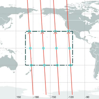
Figure 1: Groundtracks for four successive upward passes of the GRACE or GRACE Follow-On satellites across the Pacific Ocean. The circles show the locations of the assumed calibration sites in the Pacific.

At present, for GRACE data, empirical parameter corrections are used to reduce the effects of spurious accelerations. A typical procedure is to solve for once-per-revolution (once/rev) corrections to the along-track differential acceleration from each one revolution arc of data, plus a few other parameters such as the mean differential acceleration. However, a priori information on the geopotential height variations along the orbit at satellite altitude have to be used in solving for the parameters in the spurious acceleration corrections. This means that errors in the a priori geopotential height variation models will result in errors in the final GRACE results. In addition, it appears possible that the empirical parameter set solved for with present GRACE data is not sufficient to take out most of the effect of differential spurious accelerations.

An alternate approach that has been suggested (Bender et al. 2011, Bender and Betts 2013) is to make use of a priori information on geopotential height variations only over regions where such information is known substantially better than at average worldwide locations. The main candidate for an extended region with good a priori information is the low latitude region of the central Pacific Ocean. In particular, there is one period per day when four successive revolutions of the satellite pair will pass upward across the main part of the Pacific, as shown in Figure 1, and then another period when four successive revolutions will pass downward across the region. Thus the possibility of using mainly data over that region in correcting for spurious accelerations appears to be quite attractive. However, including the data from two or more passes across low latitude regions of the Atlantic and Indian Oceans during the same time intervals would be desirable. The sites from which the necessary data are obtained will be referred to as calibration sites.

To keep the situation as simple as possible, the discussion here will be limited to such four revolution arcs of data, which are assumed to start and end at the South Pole. Use also can be made of the fact that measurements can be made five times at the South Pole and four times at the North Pole during the chosen four revolution arcs for a polar orbiting satellite pair. At an altitude of about 500 km, this takes only 6.3 hours, so the geopotential heights at satellite altitude at the poles are likely to have changed little during this time. Thus multiple measurements at the poles can help in interpolating between low-latitude measurements over the oceans, even if the mean geopotential heights at the poles during the four revolutions are not accurately known a priori.

In discussing the time variations in the geopotential $V(t)$, it is useful to have a measure of the changes that has the units of distance. For this reason, the phrase “variations in geopotential height” will be used to describe those changes. These variations $h(t)$ are defined to be

$$h(t)=\frac{\delta V(t)}{g},$$ (1)

where $\delta V(t)$ is the difference of $V(t)$ from a model or constant value and $g$ is the local acceleration of gravity (Jekeli 1999).

2 General Approach

A well-known problem in the analysis of GRACE data is the tendency for striping to occur in the results, if precautions against this are not taken. Striping can be described as a correlation of the errors along meridians, so that maxima and minima in the errors form ridges in the north-south direction. It will be assumed here that a substantial part of the source of this problem is the difficulty of knowing the systematic errors in the satellite separation at frequencies near one cycle per revolution and at other low frequencies. Such once/rev and low- frequency variations can be caused by differential errors in the initial conditions for the two satellite orbits, and are continuously modified by spurious acceleration errors. The level to which these errors need to be known to be useful is far better than the accuracy achievable by GPS tracking. Thus variations at once/rev normally are at least partially filtered out from the data.

If the mission has a particular orbit and the results are analyzed, the variations in the error at once/rev and at other low frequencies during that period will lead to changing vertical displacements of the arcs of apparent geopotential heights with respect to the Earth’s center of mass. This will cause correlated errors along roughly the north-south direction in the resulting gravity field solution. Thus, it appears that providing a way to improve our knowledge of the systematic errors in separation at once/rev and at other low frequencies, and of the spurious accelerations leading to them, would be highly desirable. Testing the suggested procedure for accomplishing this is the main objective of this paper.

In investigating this problem, three major approximations will be used. One is the assumption of a very nearly spherical geopotential, with perturbations only because of short period fluctuations in the surface mass distribution. The second is the neglect of tidal effects. And the third is the energy conservation approximation.

In the energy conservation approximation (Jekeli 1999), the separation $S$ between the satellites decreases whenever they fly over a region where the geopotential height near the satellite altitude is increased. The usual statement is that the sum of the potential energy and the kinetic energy has to stay constant, to the extent that dissipative forces can be accounted for, so that for small changes in the potential energy, the velocity change will be nearly proportional to the potential change. Thus, if the potential were nearly spheroidal but with a bump in it, each of the satellites would have about the same decrease and then increase in velocity when it crossed the bump, resulting in a decrease in separation of the satellites. Thus, in principle, the changes in the geopotential height can be solved for from measurements of changes in the separation, provided that differences in the orbit parameters and uncertainties in other factors can be solved for to the extent necessary.

From Eq. (1), the energy conservation approximation can be written as

$$(\bar{v})\left[w_{2}-w_{1}\right]+g*[h_{2}-h_{1}]=0,$$ (2)

where $(\bar{v})$ is the mean velocity over the orbit, $w_{2}$ is the along-track component of the velocity for satellite 2, $g$ is the acceleration of gravity at the satellite altitude, $h_{2}$ is the geopotential height of satellite 2, etc. The main amplitudes of the geophysical time variations in the geopotential height are at degree 10 or less, so to a good approximation

$$[h_{2}-h_{1}]=\left[\frac{(\bar{S})}{(\bar{v})}\right]*\frac{dh}{dt}$$ (3)

where $h$ is the geopotential height at the midpoint between the two satellites.

Inserting (3) into (2) and integrating from $t=0$ to $t=T$ gives

$$(\bar{v})\left[S(T)-S(0)\right]+\left[\frac{(g*\bar{S})}{(\bar{v})}\right][h(T)-h(0)]=0.$$ (4)

Eqs.(2) and (4) are clearly only approximations, and thus corrections to the satellite orbit parameters and offsets of the velocity vectors from the satellite separation vector have to be allowed for in the analysis. Since $g/(\bar{v})^{2}=1/a$, where $a$ is the semi-major axis of the orbit,

$$\left[S(T)-S(0)\right]+\left[\frac{(\bar{S})}{a}\right]\left[h(T)-h(0)\right]=0.$$ (5)

If we define $\delta S$ and $\delta h$ to be the variations in $S$ and $h$ from their initial values, we have:

$$\delta S=-\frac{\delta h}{R},$$ (6)

where $R$ is given by $R=a/S_{0}$, $a$ is the orbit semi-major axis, and $R$ is about 69 for an assumed value of 100 km for the mean separation $S_{0}$. This assumed separation is about a factor of 2 less than the nominal value for the GRACE Follow-On mission, but the separation may be decreased if the laser interferometry operating mode is being used.

The geopotential height discussed throughout this paper will be that near the satellite altitude, for simplicity. Thus, after results are obtained for a given period, they will need to be downward continued to obtain the results at ground level. The downward continuation can be done by expressing the results for the geopotential at altitude in a spherical harmonic expansion, and then reducing the amplitudes to those at the desired reference surface. To be specific, the polar orbit case that is used in this paper is a nearly circular orbit with 198 revolutions in 13 sidereal days. The altitude is 489 km, and there are 15.23 revolutions per sidereal day. The offset in longitude between ground tracks on successive revolutions is 23.64^∘. Attention will be focused on measurements of the satellite separation when crossing a broad region in the Pacific Ocean between 30^∘ S and 30^∘ N latitude. The basic reason is the expected smoothness, small amplitude, and low relative uncertainty in the time variations in the mass distribution at moderate latitudes over the Pacific. The inverted barometer effect would at least partially reduce the effects of uncertainties in surface atmospheric pressure. And satellite altimetry results plus wind data derived from satellites and other sources can further reduce the uncertainty.

The orbit for GRACE does not have a fixed ground track, and neither will the orbit for the GRACE Follow-On mission. However, future missions after GRACE Follow-On seem likely to have a fixed ground track, if they are drag-free. Although such missions probably will fly at considerably lower altitudes, it was decided to use fixed ground track orbits in the present analysis. For short arc analyses, this is not expected to have any effect on the results.

The main part of this paper will be based on the expected spurious acceleration levels for the GRACE Follow-On mission. The main observables considered will be the satellite separations over 12 points in the chosen region in the Pacific, the separations at single points in the Indian and Atlantic Oceans, and those at the poles. The basic set of measurements proposed to estimate the differential spurious accelerations will be described in 3. All of the latitudes referred to in the rest of this paper will be north latitudes, and all of the longitudes will be east longitudes.

The results for the evaluation of the errors in the geopotential heights with the ocean calibration approach will be evaluated at satellite altitude along the orbit. In this way, the expected accuracy of the results can be compared with those for similar 4 revolution arcs from other approaches for correcting for the spurious accelerations of the satellites, such as various empirical parameter correction approaches, without the serious complication of the limitation from temporal aliasing. The approximation of only using calibration measurements at 12 sites over the Pacific is not expected to limit the accuracy substantially, but keeps the calculations considerably simpler.

In Sections 4, 5, and 6 the limitations on the results due to two main causes will be discussed. One limitation results from having to interpolate over periods of up to 47 minutes between the times at which measurements are made at the chosen calibration sites. The other is due to uncertainties in the a priori information on geopotential height variations with time at the calibration sites.

In Section 4, a specific choice of the interpolation procedure will be discussed. It was chosen because it does a good job of reducing the residual effects of the spurious acceleration noise. It is based on a specific model of the spurious acceleration noise as a function of frequency that is intended to be close to what will be achieved during the GRACE Follow-On mission. However, the nominal level of the spurious accelerations for the GRACE mission is only a factor of three higher, so the main results are also expected to be applicable to this case.

In Section 5, a specific, but ad hoc, model for the magnitudes of errors in the geopotential heights at the calibration sites will be described. It is based mainly on a particular model for time variations in the ocean bottom pressure in the Pacific. Then, in Section 6, the effects of the uncertainties from this model on the spurious acceleration correction proceedure will be given.

The results for this case where the expected spurious acceleration levels for the GRACE Follow-On mission are assumed appear to be quite encouraging. Thus the possibility that a similar approach could be used for some of the data from the GRACE mission will be discussed in Section 7. And finally, the general conclusions from this study of the ocean calibration approach will be reviewed in Section 8.

3 Basic Analysis Approach for Estimating Systematic Errors in the Satellite Separation

To keep the necessary calculations as simple as possible, the conceptual approach discussed here is based mainly on making use of measurements of the satellite separations when the satellites are at $-30^{\circ}$, 0^∘, and $+30^{\circ}$ latitude over the Pacific and when they are at the South Pole or the North Pole during the same four-revolution arc. With the assumed 13 sidereal day repeat satellite orbit, there will be four successive upward passes of the satellites from $-30^{\circ}$ to $+30^{\circ}$ latitude each day that will cross the equator in the Pacific Ocean between the longitudes of about 150^∘ and 245^∘. These passes will be followed about six hours later by four downward passes from $+30^{\circ}$ lat to $-30^{\circ}$ lat, where the equator crossings are in the same range of longitudes. Thus the major portions of these passes will be fairly well away from the regions of strong western or eastern boundary currents.

In addition, recent studies of uncertainties in geopotential heights over the oceans indicate that the uncertainties over the equatorial region of the Indian Ocean and a substantial range of latitudes in the Atlantic are similar to those in the equatorial Pacific (see Figure 1 in Quinn and Ponte 2011). From the geometry, it is possible to include two additional measurements near the equator over these oceans on most data arcs, one in the Indian Ocean on the first of the four revolutions and a second measurement during the last revolution over the Atlantic. Such additional data will be represented here by assuming additional calibration points when crossing the equator during the first revolution in the Indian Ocean and during the fourth revolution when crossing the Atlantic.

Finally, as discussed earlier, measurements at the South Pole and at the North Pole during the same 4-revolution arc will be included. This gives a total of 23 calibration points during each four-revolution data arc, including 12 in the Pacific, 1 each in the Indian and Atlantic Oceans, 5 at the South Pole, and 4 at the North Pole.

If there were no uncertainty in the geopotential height variations at the calibration points in the oceans or at the South or North Pole during the four revolution period, the variations in the satellite separation $S$ due to the spurious accelerations could be interpolated from the measured separations at the reference locations. However, the choice of what type of interpolation function to use requires some care because of the along-track spatial gaps of up to 180^∘between some of the measurements. Because 23 measurements at the calibration points are included during the four revolutions, up to 23 basis functions could be used to fit the reference point data. However, it has been found in this study that least squares fitting on a substantially lower number of basis functions works better.

The reason for this result is that there actually will be differential noise in the knowledge of geopotential height variations at calibration points in the Pacific that are separated by fairly short distances, down to below 21^∘. To fit such variations, basis functions with quite short wavelengths are needed, and they can amplify the effects of the geopotential height uncertainties when applied to the regions where substantial interpolation is needed. Thus the number of basis functions used generally has been limited to about two-thirds of the number of calibration points.

For convenience, the locations of the reference points are given in terms of the angular motion along track of the satellites with respect to the South Pole crossing at the center of the four revolution arc of data. Thus they range from $-720^{\circ}$ to $+720^{\circ}$. The crossings of $-30^{\circ}$, 0^∘, and $+30^{\circ}$ latitudes in the Pacific for data sets with upward passes there will occur at $-660^{\circ}$, $-630^{\circ}$, $-600^{\circ}$ during the first revolution, etc.

The first error source to be considered is the result of incomplete correction for the differential spurious acceleration noise between the two satellites. It is assumed that equal weight will be given to the difference between the observed value and the value of the geopotential height at satellite altitude that is used at each of the calibration sites. Then, if the a priori value at the $i$-th calibration site is $Y_{i}$, an approximation function for the $Y_{i}$ can be defined in terms of M basis functions $X_{j}(\theta_{i})$ by

$$\vec{Y}(\theta)=\Sigma_{j}{(a_{j})[X_{j}(\theta)]}.$$ (7)

If a trial set of M basis functions is chosen, plus a set of $N$ calibration points, the best fitting set of coefficients $a_{j}$ can be chosen by the least squares approach. The function $\vec{Y}(\theta)$ that results from least squares fitting the coefficients $a_{j}$ will be called the correction function, or the interpolation function.

The starting point for the analysis is a $N\times M$ matrix A, called the “design matrix”. Here A$(i,j)$ is the value of the $j$-th basis function at the $i$-th calibration point. If a vector $\vec{Y}$ of the apparent geopotential height errors $Y_{i}$ at the $i$-th measurement site is assumed, and ${\bf\rm H}=[{\bf\rm A}^{T}]*A$, then the vector $\vec{Z}$ of least squares fitted coefficients of the basis functions is given by

$${\vec{Z}}=[{\bf H}^{-1}]*[{\bf A}^{T}]*\vec{Y}={\bf K}*\vec{Y},$$ (8)

where this equation defines the matrix K. The asterisk represents vector or matrix multiplication.

In order to compare different possible choices of the basis functions, a specific criterion is needed. To keep the calculations fairly simple, the criterion used here is based on just considering the residual noise after correction at the times during the four revolutions when the satellites are on the opposite side of the orbit from the Pacific, at latitudes of 60^∘, 30^∘, $-30^{\circ}$, and $-60^{\circ}$. This set of points will be called the evaluation points, and the results for the specific choice of the basis functions that has been used will be discussed in Section 4.

4 Imperfect Interpolation of the Satellite Separation Noise

4.1 Basic Approach

The results of the choice of basis functions clearly depend on the spectral amplitude of the noise in the satellite separation due to the spurious accelerations. It will be assumed here that the rms acceleration noise for each satellite in the Grace Follow-On mission is $3.3\times 10^{-11}$ m/s${}^{2}/\sqrt{{\rm Hz}}$ (Foulon et al. 2013) in both the along-track and radial directions from 0.005 Hz to 0.1 Hz, and that it increases as $[0.005/f]^{0.5}$ at lower frequencies. With these assumptions, the resulting noise in the along-track separation of the satellites can be calculated by integrating twice with respect to time, and then correcting for the resonance with the orbital frequency at 1 cycle per revolution (cy/rev).

Table 1: Spurious acceleration noise estimates for the GRACE Follow-On mission

Nominal	Sep. Noise	Resonance	Total	Equivalent
Frequency	Amp. Without	Factor	Sep. Noise	Geopotential
(cy/rev)	Res. Factor		Amplitude	Height Error
	($1\times 10^{-6}$ m)		($1\times 10^{-6}$ m)	(mm)
3/64	2810	3.0	8430	582
1/8	723	3.1	2240	156
1/4	75.3	3.3	249	17.1
29/64	27.9	4.6	129	9.00
5/8	4.62	5.9	27.3	1.89
11/16	3.63	7.9	28.8	1.98
3/4	2.92	9.9	29.1	2.01
13/16	2.39	11.0	26.4	1.83
7/8	1.99	12.1	24.0	1.65
15/16	1.67	12.7	21.3	1.47
1	1.42	12.9	18.3	1.26
17/16	1.22	12.7	15.6	1.08
9/8	1.06	12.1	12.9	0.90
19/16	0.924	11.0	10.2	0.69
5/4	0.813	9.9	8.10	0.558
21/16	0.720	8.1	5.82	0.402
11/8	0.639	6.3	4.02	0.276
23/16	0.573	5.6	3.21	0.222
3/2	0.516	4.8	2.46	0.171
25/16	0.465	4.4	2.04	0.141
13/8	0.420	4.0	1.68	0.117
27/16	0.384	3.7	1.41	0.096
7/4	0.351	3.4	1.20	0.084
29/16	0.321	3.2	1.02	0.069
15/8	0.294	3.0	0.87	0.060
31/16	0.27	2.8	0.75	0.051
2	0.252	2.6	0.66	0.045

With these assumptions, the resulting noise in the along-track separation of the satellites without including the effect of the orbital resonance is given in the second column of Table 1. These values are for the root mean square noise amplitudes for 27 frequency intervals centered on the nominal frequencies given in column 1. They range from 3/64 to 2 cy/rev. The bandwidths are 1/32, 1/8, 1/8, and 9/32 cy/rev for the lowest four frequencies, and are 1/16 cy/rev for the rest. The sum of the frequency intervals chosen covers the range from 1/32 to 65/32 cy/rev uniformly.

Rough estimates of the effect of the orbital resonance on the satellite separation were obtained as follows. The Hill equations (Kaplan 1976) were used to calculate the effect of a given low level of along-track perturbing force on one of the two GRACE satellites on the range between the satellites during four revolutions. This was done for different perturbing frequencies, and the ratio of the rms range change to that for frequencies way above the orbital frequency was taken as the resonance factor for the along-track perturbations. Then the same was done for radial perturbing forces. The rss (root sum square) combination of these factors is listed as the resonance factor in column 3 of Table 1.

Finally, the error in the geopotential height at satellite altitude that would result from this separation noise level is obtained by multiplying by a factor 69, as discussed in Section 2, and is given in the fifth column. These rms amplitudes are called $q(k)$, where $k$ is the index number for the $k$-th noise frequency. The amplitudes are large at frequencies below 5/8 cy/rev, but with suitable choices of basis functions, it was found that the contributions to the interpolation errors for the different frequency intervals could be made to decrease at the lowest frequencies.

The corresponding sine and cosine functions used to represent the range noise at specific frequencies will be called $ws_{k}(t)$ and $wc_{k}(t)$, with $ws_{1}(t)$ and $wc_{1}(t)$ being the sine and cosine functions for the first noise frequency, $ws_{2}(t)$ and $wc_{2}(t)$ those for the second noise frequency, etc. The maximum amplitudes of the noise functions are 1, except for the sines of any frequency less than 1/8 cy/rev. The values of the noise functions at the calibration points are given by matrices BS and BC, where ${\rm BS}(i,k)$ is the value of the $k$-th sine noise function at the $i$-th calibration point and ${\rm BC}(i,k)$ is the value of the $k$-th cosine noise function at the $i$-th calibration point.

Let $\bf{CS}={\bf K}*{\bf BS}$ and ${\bf CC}={\bf K}*{\bf BC}$. Then CS$(i,k)$ and CC$(i,k)$ are the amplitudes of the $i$-th basis function coefficients due to unit amplitude for the $k$-th sine and cosine noise functions. Also, let J$(m,i)$ be the amplitude of the correction function at the $m$-th evaluation site due to a unit coefficient for the $i$-th basis function. And, let the matrices ${\bf DS}(m,k)$ and ${\bf DC}(m,k)$ be the values at the $m$-th evaluation site due to unit amplitude for the $k$-th sine and cosine noise functions. Then, if the matrices ${\bf ES}={\bf J}*{\bf CS}-{\bf DS}$ and $\bf{EC}={\bf J}*{\bf CC}-{\bf DC}$, then ${\bf ES}(m,k)$ is the error in the correction function at the $m$-th evaluation site due to a unit error in the $k$-th sine noise function, etc.

Let $k=1$ to 4 correspond to the evaluation points at along-track angular locations of $-510^{\circ}$, $-480^{\circ}$, $-420^{\circ}$, and $-390^{\circ}$ with respect to the mid-point of the four-revolution arc, $k=5$ to 8 correspond to $-150^{\circ}$, $-120^{\circ}$, $-60^{\circ}$, and $-30^{\circ}$, etc. The different realizations of the noise function for different sets of four revolutions on different days can be evaluated by randomizing the signs of the amplitude coefficients $q(k)$ of the noise functions. If the values of the $q(k)$ are those given in Table 1, then the square of the error in the correction function at the $m^{\rm th}$ evaluation point due to the rms error $q(k)$ in both the sine and cosine noise functions for the $k^{\rm th}$ noise frequency is given by

$${\rm E}(m,k)=[q(k)*{\rm ES}(m,k)]^{2}+[q(k)*{\rm EC}(m,k)]^{2}.$$ (9)

For a given set of basis functions, E$(m,k)$ contains all of the information needed to evaluate how well the resulting least squares fit correction function will do in minimizing the mean square errors at the 16 chosen evaluation sites in the hemisphere opposite to the Pacific.

4.2 Results

Table 2: Mean square interpolation error at the 16 evaluation sites

Eval. site #	1	2	3	4	5	6	7	8	9	10	11	12	13	14	15	16
Error (mm2)	0.549	0.234	0.261	0.738	2.05	2.91	2.41	1.27	0.855	1.85	2.50	1.66	0.963	0.459	0.810	1.63

The investigation of different choices of basis functions for the interpolation process consisted of calculating the matrix E$(m,k)$, and looking at the amplitudes in its different columns. From these amplitudes, the contributions to the geopotential height uncertainty due to the interpolation process can be seen for each frequency interval separately. Thus changes in the choice of basis functions can be considered, based on what frequency regions appear to need better coverage.

With the estimates of amplitude coefficients $q(k)$ given in the fifth column of Table 1, several different combinations of up to 16 basis functions were chosen to try to fit the noise at the calibration points in such a way that the residual noise at distant locations would be small. As discussed earlier, the criterion used was to minimize the residual noise at the times during the four revolutions when the satellites were at the 16 chosen evaluation points. With this criterion, a reasonable choice of M basis functions was found to be as follows: $X_{1}=1$ and $X_{2}=\theta/4\pi$, where $\theta$ is the angular position with respect to the center of the four-revolution arc; $X_{3}$ to $X_{8}$ are the sines of 5/4, 1, 3/4, 7/16, 7/32, and 13/128 cy/rev; $X_{9}$ to $X_{14}$ are the cosines of these frequencies; $X_{15}$ is a function that is 1 at the times of crossing the South Pole and is 0 at other times; and $X_{16}$ is similarly defined for the North Pole.

For this set of basis functions, the matrix E$(m,k)$ was calculated. From it, the values of F$(m)$ were obtained, where F$(m)$ is the sum of E$(m,k)$ over $k$. The values of F$(m)$ are the mean square interpolation errors at the individual evaluation sites that would be obtained if there were no errors in the knowledge of the geopotential heights at the calibration sites. They are given in Table 2.

The average of F$(m)$ over the 16 evaluation sites is $<{\rm F}(m)>=1.32$ mm². Thus the expected root mean square error in the correction function at the evaluation sites due to the interpolation process is 1.15 mm in the geopotential height at satellite altitude.

As will be seen later, this measure of the rms error due to interpolation of the correction function for the spurious acceleration noise is quite small compared with the effect of uncertainties in the geopotential height time variations at the calibration sites. However, it is of some interest to see if a simpler set of basis functions could produce nearly as small an error due to interpolation. As a measure of this, the calculations were repeated for 6 different cases. In each, one of the six basis function frequencies was left out, so that only 14 basis functions remained. The results were that in each case the overall rms interpolation error increased by a factor of 2 or more. Thus it appeared worthwhile to keep all 16 of the basis functions in the remaining parts of the study.

Also of interest is how the expected mean square errors over the evaluation sites vary with the noise frequency. To see this, the average of E$(m,k)$ over $m$, ${\rm G}(k)=<{\rm E}(m,k)>$, is given in Table 3 for the 27 different noise frequencies considered.

Table 3: Mean square error in geopotential height for different noise frequency bands

Freq. (cy/rev)	3/64	1/8	1/4	29/64	5/8	11/16	3/4
Error (mm2)	5e-6	3e-6	3e-6	0.001	0.001	0.001	4e-18
Freq. (cy/rev)	13/16	7/8	15/16	1	17/16	9/8	19/16
Error (mm2)	0.001	0.010	0.003	6e-14	0.005	0.271	0.015
Freq. (cy/rev)	5/4	21/16	11/8	23/16	3/2	25/16	13/8
Error (mm2)	2e-19	0.020	0.065	0.135	0.171	0.185	0.160
Freq. (cy/rev)	27/16	7/4	29/16	15/8	31/16	2
Error (mm2)	0.112	0.078	0.033	0.028	0.016	0.011

The error contributions for 3/4, 1, and 5/4 cy/rev are less than 10^-13 mm², since these are three of the basis function frequencies. Also, the error contributions are very small for the frequency bands from 3/64 to 1/4 cy/rev. The main peaks are at 7/8, 9/8, and 25/16 cy/rev, and the errors go down smoothly for frequencies above 25/16 cy/rev.

At an early stage in the processing of real data, the 16 parameters in the correction function for a particular 4 revolution arc would be determined. Then, this correction to the satellite separation during the arc would be made, before the main part of the processing. The processing could be done either in terms of the range or the range rate, since sufficiently precise numerical proceedures for either approach are now available (Daras et al. 2015).

5 Errors in the Geopotential Heights at the Calibration Sites

5.1 Model for the Errors

As emphasized by Quinn and Ponte (2011) in a recent paper: “Knowledge of variability in ocean bottom pressure at periods $<60$ days is essential for minimizing aliasing in satellite gravity missions.” Among the best of the currently available detailed models for variations in the properties of the oceans are the models produced by the Estimating the Circulation and Climate of the Ocean consortium (the ECCO models) (Wunsch et al. 2009). Results from a particular one of these models, called dr080, are available at the ECCO-JPL website (http://ecco.jpl.nasa.gov/ external). Among the results are the ocean bottom pressure variations at a grid of points covering almost all of the oceans. We use these results in this paper to estimate the variations in the geopotential at sites in the central part of the Pacific. This model includes assimilation of data from the oceans.

Results for ocean bottom pressure variations in the ECCO model at a number of sites in different oceans where there are ocean bottom pressure gauges, as well as comparisons of these two measures of variations, have been given in Quinn and Ponte (2011). Also included are comparisons with variations from an alternate ocean circulation model at these sites. These results were most encouraging for the North Atlantic and the eastern part of the Pacific. Our results in a later part of this paper will be compared with the Pacific results of Quinn and Ponte (2011).

The model we are using for the geopotential height variations at 500 km altitude at the calibration sites in the Pacific has four components: (1) random variations at each of the sites at the calibration times; (2) a uniform offset at all of the sites during the roughly 6 hour calibration period; (3) a north-south gradient during this period across the area covered by the calibration sites; and (4) an east-west gradient across the area during this period. While this model is quite crude, we believe that it will give a fairly good description of how the geopotential variation uncertainties will affect the acceleration correction approach we are pursuing if the amplitudes of the four terms listed above are well chosen.

As a basis for estimating the parameters to use in the geopotential variation uncertainty model, it would be desirable if we could start from knowledge of the uncertainties at different locations over some period of time. However, there are limits on how well those uncertainties are known. One check would be to compare the results from the ECCO-JPL model with the geopotential variation results from present analyses of data from the GRACE mission. However, since errors in the anti-aliasing geopotential models over both land and oceans used in analysis of the GRACE data can affect the GRACE results substantially, it seems quite possible that the comparison would not give a useful evaluation of the actual uncertainty in the geopotential variation information available from sources other than the GRACE data.

In view of the above, we decided to start by looking at the full geopotential variations predicted by the ECCO-JPL model. The way in which this was done is described in the next section.

5.2 Geopotential Variations at Satellite Altitude from the ECCO-JPL Model

The quantity of interest in calculating variations in the geopotential at satellite altitude are the variations in the mass per unit area as a function of latitude, longitude, and time. Since short wavelength variations in the mass are attenuated rapidly with altitude, we chose to use the variations in bottom pressure from the ECCO-JPL model only at a grid of points separated by about 3^∘ in both latitude and longitude. The points included were most of those at 3^∘ intervals which were ocean points between $-60^{\circ}$ and $+60^{\circ}$in latitude and between 135^∘ and 285^∘ longitude, and not east of Mexico or Central America. The bottom pressure results at 0 and 12 hours UT during December 2010 were used.

To provide a check on the values at each grid point, we first subtracted the mean for the month and then calculated the rms variations from the mean. The large majority of the rms values were less than 3.0, in cm of water, and grid points with values greater than this have not been included in the calculations. In addition, 120 grid points with values between 2.0 and 3.0 were excluded, and 14 with values less than 2.0. These were mostly at latitudes between $-60^{\circ}$ and $-48^{\circ}$ and between $+36^{\circ}$ and $+45^{\circ}$ , where the variability appeared to be much greater than at lower latitudes. These points were excluded because of their variability being substantially higher than for the typical grid points within 35 degrees of the equator, which contributed most of the variations according to the ECCO-JPL model, and thus not being representative of how the model would be used in practice. This left about 1360 grid points to be used in the calculations.

The next step was to use the differences from the mean for the month for all the included grid points at a given latitude to calculate directly their contribution to the geopotential height variation at satellite altitude at each of the 12 calibration points. These were chosen to be at latitudes of $-30^{\circ}$ , 0^∘, and $+30^{\circ}$ , and at east longitudes of 234^∘, 211^∘, 188^∘, and 165^∘. For actual satellite passes northward across the Pacific, the longitudes would be about 2 degrees higher at $-30^{\circ}$ and 2^∘ lower at $+30^{\circ}$ N. However, these offsets would be reversed for southward passes, and these differences are not likely to be large enough to affect the geopotential variation model results appreciably. Also, on different days, the longitudes of the passes across the Pacific would be shifted by up to about 12^∘ in either direction, but not including these shifts is not expected to make a substantial effect on the results. Including them would make the calculations considerably more complicated.

For the contributions from each latitude band of grid points and for each of the 62 times during the month, the results at the 12 calibration sites were inspected to look for outliers. However, the results appeared to vary quite smoothly with latitude and with time. Thus the total variations from all of the latitude bands at each time were calculated. This gave the values as a function of time shown in Figure 2, in units of millimeters of geopotential height at satellite altitude. The values for the times during the month and the various calibration sites range from $-$2.8 mm to 3.3 mm.

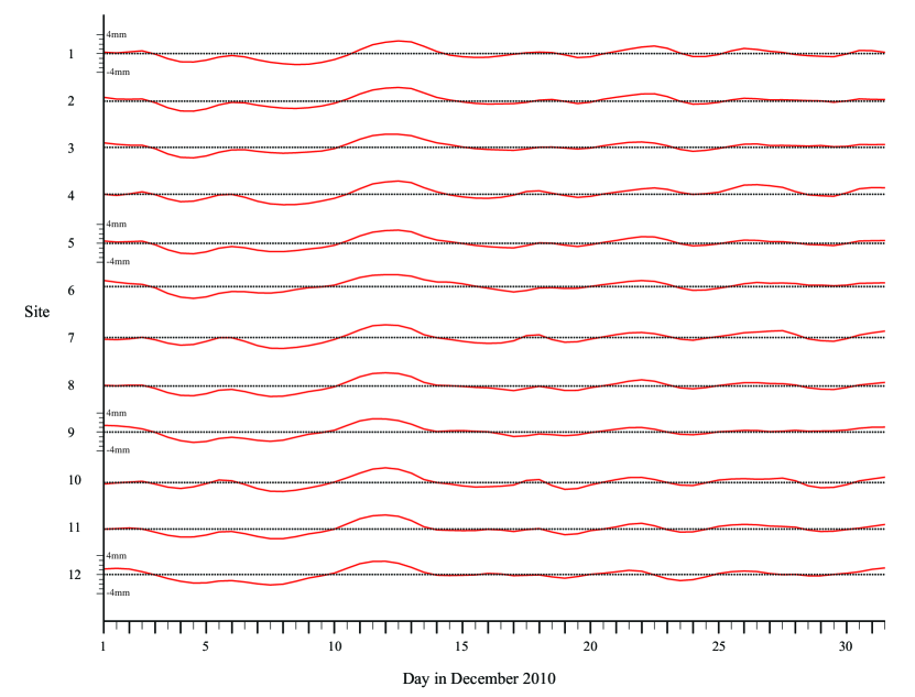
Figure 2: Variations at the 12 calibration sites in the geopotential height at satellite altitude from the ECCO-JPL ocean model.

5.3 Further Analysis of Geopotential Variation Results from ECCO

In order to investigate the statistics of the variations shown in Figure 2, we calculated the rms values over time for each calibration site. These values ranged from 0.99 mm to 1.28 mm. The rms value for all of the calibration sites is 1.15 mm. A comparison with the corresponding rms values over the whole globe for the anti-aliasing geopotential variation models used in analysis of the GRACE results, or the difference between two such models, certainly would be of interest. It is expected that the global rms values would be higher, because of the larger expected uncertainties at high latitudes over the oceans and over much of the land areas (see e.g., Thompson et al. 2004 and Gruber et al. 2011).

However, comparing with the rms values of the anti-aliasing geopotential variation models over the rest of the globe might well not give a useful measure of how much improvement could be obtained with the ocean calibration approach. The reason is that the uncertainties in the global anti-aliasing models are the important quantities, and these are not well known.

Other subjects of interest besides the rms values over all the calibration sites are the variations in the average value over all 12 sites during the month and the variations in the north-south and east-west differences across the Pacific calibration area across the set of calibration sites. The average values over all 12 sites range from $-$2.00 mm to 2.81 mm. The rms of these values is 1.08 mm. The variations in the average values over the 12 calibration sites are of considerable interest because the resulting contributions from the correlated variations won’t be reduced in the way that the uncorrelated variations would be.

The variations with time in the north-south and east-west differences across the area covered by the calibration sites also can have substantial effects. As a measure of the north-south differences, we take the difference at each time between the averages of the values at the sites at $+30^{\circ}$ and those at $-30^{\circ}$. These values range from $-$1.28 mm to 1.35 mm, with an rms value of 0.63 mm.

For a rough measure of the east-west differences across the Pacific calibration area, we take the sum of the following: the average of the values at 234^∘ minus the average of those at 165^∘, plus one third of the average of the values at 211^∘ minus those at 188^∘. These values at the different times range from $-$1.09 mm to 1.50 mm. The rms of these values is 0.62 mm. If the geopotential height varied linearly across the area, this estimate would be slightly pessimistic compared with the total geopotential height change across the $71^{\circ}$ width of the area at the equator.

These values for the rms variations in the geopotential heights at the individual calibration sites, the averages over the calibration sites, and the differences across the calibration sites, are expected to be substantially larger than the errors in these quantities. However, we have used them to provide an intentionally somewhat pessimistic model for the errors in these quantities. If no better information on the expected model errors becomes available, these values can be used as the basis for a model of the geopotential height variation uncertainties to be used in the ocean calibration approach to correcting for spurious accelerations in future GRACE-type missions, like the GRACE Follow-On mission, and possibly for GRACE itself. However, before discussing this application of the results further, a partial comparison of the ECCO model results with another source of information on ocean mass distribution changes will be described.

5.4 Comparison with Ocean Bottom Pressure Gauge Results

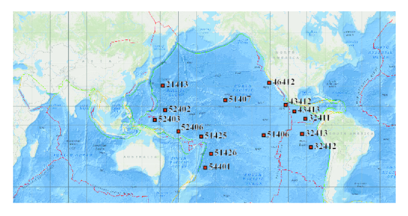
Figure 3: Locations of the NOAA Deep-ocean Assessment and Reporting of Tsunamis (DART) ocean bottom pressure gauges used in the comparison with values from the ECCO-JPL ocean model.

As a partial check on the ECCO results for ocean bottom pressure variations, we have made a comparison with data from 15 of the ocean bottom pressure (BPR) gauges in the NOAA Deep-ocean Assessment and Reporting of Tsunamis (DART) network. About 35 of these BPR gauges are located in the Pacific, with about half located fairly near the west coasts of North, Central, and South America plus along the Aleutian arc. Most of the rest are located in the western part of the Pacific.

Current results from the gauges are available on the website www.ngdc.noaa.gov/hazard/DARTData.shtml. However, these results include the quite large variations due to the tides. We fortunately were able to obtain results that had been corrected for the tides from the NOAA National Geophysical Data Center. The data we obtained were 3 hour average values every 12 hours during December 2010 for 15 of the DART sites. The variations in bottom pressure were then converted to variations in equivalent water depth, and the means for the month were subtracted. Similar results were obtained for one of the ECCO grid points close to each of the DART sites.

Table 4: Locations of the DART and ECCO sites

DART sites			ECCO sites
Site	Lat	Long	Nor.	East	Nor.	East
			Lat	Long	Lat	Long
			Gr#	Gr#
21413	30.51	152.12	175	152	30.5	152.5
32411	5.00	269.16	129	269	5.1	269.5
32412	-17.96	273.61	62	273	-18.05	273.5
32413	-7.40	266.50	87	266	-7.5	266.5
43412	16.07	253.00	159	252	15.82	252.5
43413	11.06	260.15	149	260	11.12	260.5
46412	32.46	239.44	177	239	32.5	239.5
51406	-8.48	234.97	84	234	-8.4	234.5
51407	19.59	203.42	164	203	19.75	203.5
51425	-9.51	183.76	80	183	-9.6	183.5
51426	-22.99	191.87	57	191	-22.54	191.5
52402	11.87	154.04	151	154	11.79	154.5
52403	4.05	145.59	126	145	4.2	145.5
52406	-5.29	165.00	94	165	-5.4	165.5
54401	-33.00	187.02	47	187	-32.5	187.5

The DART sites included are shown in Figure 3. They also are listed in Table 4, along with the locations of the nearby ECCO model grid sites. The Dart sites ranged in latitude from $-$33.00^∘ to $+$32.46^∘ and in longitude from 145.59^∘ to 273.61^∘. This range of locations was chosen to stay away from high latitudes and from western or eastern boundary current regions. DART site #46412 is located quite close to the Southern California coast, but it was included because of the lack of other DART sites in the northeastern corner of the region of interest.

The results of the comparisons of the DART and ECCO variations are given in Table 5. For each DART site, the rms values of the differences from the mean are given for that site and for the nearby ECCO site. In addition, the correlation coefficient $\rho$ between the variations from the two sources is given.

Table 5: Comparisons of the DART and ECCO rms water height variations

DART	DART $\sigma$	ECCO $\sigma$	Corr.
Site	(cm)	(cm)	Coeff.
21413	2.42	2.16	0.852
32411	1.08	0.75	0.494
32412	1.32	0.80	0.579
32413	1.36	0.62	0.594
43412	1.32	0.75	0.659
43413	1.52	0.62	0.500
46412	1.37	0.62	0.379
51406	1.38	0.74	0.767
51407	1.56	0.77	0.429
51425	1.41	0.57	0.444
51426	1.63	0.61	0.580
52402	1.86	0.86	0.552
52403	1.42	0.82	0.584
52406	1.17	0.62	0.428
54401	2.39	1.38	0.726

It is interesting that the first and last of the sites listed have substantially larger rms variations in equivalent water depth, both for the DART and ECCO results. The correlation coefficients at these sites have 2 of the 3 largest values for all the sites. Also, 14 of the 15 sites have correlation coefficients above 0.40. Thus there is a substantial contribution to the results that is common between the two sets of measurements.

At essentially all of the DART sites, the rms variations in the DART results are very roughly twice the size of the rms variations in the ECCO results. This is likely to be due to a combination of the noise in the DART results being higher than for the ECCO model and the variations in the ocean bottom pressure in the ECCO model being somewhat smaller than the real variations. Since the correlation coefficients between the two types of variation results are typically about 0.5, there is enough correlation to suggest that the magnitude of the actual variations is somewhere in between.

In the paper mentioned earlier (Quinn and Ponte 2011), the ECCO data were compared with ocean bottom pressure gauge (BPR) data and with another ocean model at gauge locations in the Atlantic and Indian Oceans, as well as in the Pacific. The other ocean model used was the Ocean Model for Circulation and Tides (OMCT), that has been used as a de-aliasing model for GRACE data. They found that the variance was only about 1 cm² of equivalent water depth variation in the Pacific. The correlations of BPR results with the ocean model results had a wide range of values, but with values of 0.3 or more at many sites. The rms variations for the BPR data in the eastern Pacific were only 2 to 2.5 cm, which is consistent with the variations found in this paper.

Our results and those of Quinn and Ponte don’t give direct estimates of the uncertainty in the mass distribution variations in the ECCO model. However, it seems unlikely that the uncertainty is appreciably larger than the variations in the model. The uncertainty also could be substantially smaller, without this being apparent from the comparisons that have been done.

In view of the above, we have made what we regard as somewhat conservative estimates of the values to use in our model for the four types of errors for the Pacific sites included in model. The estimated errors are as follows: (1) 1.5 mm for the random errors at each of the Pacific calibration sites; (2) 1.5 mm for the common error at the sites during the 4 revolution observation period; (3) 1.0 mm for the N-S gradient; and (4) 1.0 mm for the E-W gradient. For (1) and (2), the value chosen is about 35% higher than the rms value for the ECCO data, to allow for the possibility of that model actually not including some of the real ocean variability. For (3) and (4), the values chosen are near the maximum values found from the ECCO data for a similar reason.

As emphasized earlier, the uncertainties in geopotential height time variations are believed to be less over relatively low latitude regions in the oceans than over land or at higher latitudes. However, to evaluate the effect of these uncertainties, some sort of model for them is needed. What has been done in the past is to take two different models for the variations in the ocean mass distribution with time, and compare their results, or to compare one model against other types of data. The problem with comparing different models is that they share some of their input data, and thus their errors may be considerably correlated. For comparisons against other types of data, the problem is the limitation of coverage of data from other sources, except for comparisons of the ocean surface height variations with altimetry results.

As an alternate approach, it was decided to evaluate the variations in geopotential height at satellite altitude according to one ocean model, and then assume that the uncertainty is equal to some fixed fraction of the variations obtained from the ocean model.

6 Errors due to Uncertainties in Estimation of the Geopotential Height Variations at the Calibration Sites

Although the situation would be slightly different for four revolution arcs with downward crossings across the Pacific from those with upward crossings, the results are expected to be nearly the same. Thus only the upward crossing case has been studied. Also, the choice of measurements at only three latitudes in the Pacific is clearly not realistic, but it is expected that it will give a good indication of what to expect. The errors in geopotential height estimates are expected to be quite well correlated over distances considerably less than 30^∘.

Our simplified error model based on uncertainties in the geopotential heights at satellite altitude is summarized in Table 6. For the sites in the Pacific, a correlated error of 1.5 mm is assumed for all 12 sites, plus random 1.5 mm errors. In addition, an error of 1.0 mm amplitude is assumed for the N-S gradient between the sites at 30^∘ N and those at 30^∘ S, and a 1.0 mm error for the E-W gradient. For the remaining sites, random errors of 2.5 mm are assumed for the Indian and Atlantic Ocean sites, which is similar to the rss of the different errors at a given Pacific Ocean site. And random errors of 0.5 mm for each of the four North Pole and five South Pole observations are included, to allow for the variations during the times between those observations.

A study of the variability of the geopotential height over favorable low-latitude sites in the Atlantic and Indian Oceans based on the ECCO-JPL model has not been carried out. However, from Figures 1b and 1c in Quinn and Ponti (2011), it does not appear that the variability at such sites would be substantially worse than at central Pacific sites. Also, from their Figure 2b, the difference between the OMCT ocean model and the ECCO model appears to be fairly small for both the Atlantic and Indian Ocean sites. Thus it seems reasonable to adopt 2.5 mm as the estimate for the variability for the calibration sites in these locations.

Table 6: Ad hoc error model for the geopotential height variation uncertainties

Pacific sites:
Uniform error at 12 sites:	1.5 mm
Random error at sites:	1.5 mm
Linear N-S variations:	1.0 mm
Linear E-W variations:	1.0 mm
Random errors at Indian
Ocean and Atlantic Ocean sites:	2.5 mm
Random errors at North
Pole and South Pole crossings
due to time variations:	0.5 mm

To give some indication of the scale of the errors assumed in the error model, it is useful to consider the change in geopotential height at satellite altitude due to a Gaussian disk of water with 1 cm height at the center and a half-mass radius of 39^∘. This much additional water would increase the geopotential height by 1.0 mm, equal to two-thirds of the correlated and the random error assumed at the Pacific sites. However, validation of the assumptions in the error model will require improved evaluations of the uncertainties in present ocean circulation models and their correlations over the distances between the chosen calibration sites, as discussed in Section 5.1.

It should be noted that the uncertainties in the geopotential time variations assumed here are equal to all of the time variations from the ECCO-JPL model. This may be regarded as a fairly pessimistic assumption, since the uncertainties actually could be substantially less. However, it is difficult to find evidence for the model being better than this over the time scales of interest. Comparisons with ocean bottom pressure gauge results from the DART network, as discussed earlier, indicate that the uncertainties aren’t likely to be substantially worse than assumed. But the noise level in those data is large enough to prevent a more precise comparison from being made.

The final step in the evaluation of the ocean calibration approach was to use the set of 16 basis functions discussed in Sec. 4.2 along with the ad hoc geopotential height variation error model to see how large the resulting errors in the correction function at the evaluation sites would be. If a particular case of the error model from Table 6 is chosen, such as the common error of 1.5 mm at the 12 Pacific sites, this defines the vector $\vec{Y}$ of geopotential height errors described just before eq. 3 in Section 3. Then, if K is the matrix defined in eq. 4 and J is the matrix defined in Section 4.1, the resulting errors at the 16 evaluation sites will be given by the vector $\vec{L}$, where

$$\vec{L}=\vec{J}*\vec{K}*\vec{Y}$$ (10)

The calculation of $\vec{L}$ is repeated for each of the independent errors in Table 6, and the squares of the 16 entries in each resulting vector $\vec{L}$ are averaged to give the mean square error at the evaluation sites due to the errors in the ad hoc error model. The resulting contributions to the average mean square error at the evaluation sites are given in Table 7.

Table 7: Average mean square errors at the evaluation sites in mm²

Independent errors at the Pacific sites:	1.62
Common error at the Pacific sites:	0.10
North-south variations:	2.01
East-west variations:	0.29
Indep. error at Indian site:	2.74
Indep. error at Atlantic site:	1.10
Indep. errors at Pole crossings:	0.42
Total (mm2)	8.28

With the contribution of 1.32 mm² from the spurious acceleration noise, this gives a mean square error of 9.60 mm² at the evaluation sites, or an rms error of about 3.1 mm. If the values in the geopotential variation error model were half as large as assumed, the rms error at the evaluation sites would be reduced to about 1.8 mm. These values appear to give a reasonable range for the estimated geopotential height uncertainties from the GRACE Follow-On mission, if other comparable or larger sources of low-frequency range uncertainty do not show up in the data.

It unfortunately is true that only about half of each day would be covered by the 4 revolution arcs that cross the central Pacific. Thus, other approaches to correcting for spurious accelerations or other low frequency errors would have to be used the rest of the time. However, these other approaches could be compared with the results from ocean calibration during the 4 revolution arcs that do cross, in order to possibly help in determining which of the other approaches to use the rest of the time.

7 Possible Application to GRACE Data

For the GRACE mission, the acceleration noise level requirements were a factor of 3 less severe than for GRACE Follow-On. Thus, the overall requirement on the range acceleration noise level due to the accelerometers in the two satellites was

$${\rm PSD}^{1/2}<3\times 10^{-10}\bigg{[}1+\frac{0.005\ \rm Hz}{\rm f}\bigg{]}^{0.5}{\rm m}/{\rm s}^{2}/\sqrt{{\rm Hz}}$$ (11)

Based on this nominal acceleration noise level for GRACE, the mean square contribution to the geopotential height uncertainty at the evaluation sites would be 12 mm². With the 8.3 mm² contribution from the uncertainties in the geopotential heights at the calibration sites, this gives a total mean square uncertainty of 20.3 mm² at the evaluation sites, or an rms uncertainty of 4.5 mm. This is just a factor 1.5 higher than was found earlier for GRACE Follow-On.

In view of this result, it appears useful to consider the possibility that the ocean calibration approach could be tested using selected subsets of the GRACE data. But, unfortunately, it is difficult to tell how much of a change this approach might make, since a number of other error sources are present besides the nominal level of accelerometer noise. The sources of real or apparent extra low-frequency range acceleration noise in the early GRACE data were discussed quite early by Flury et al. (2008), and in other papers that they refer to. One of these sources is related to the fairly frequent thruster firing for attitude control. A second is short mechanical disturbances called twangs that are triggered by temperature changes somewhere in the satellite, and a third is short pulses apparently due to electrical disturbances.

Flury et al. (2008) were able to find some periods of 70 to 300 seconds during which none of these disturbances appeared to be present. Based on the data from such periods, they concluded that the different components of the acceleration noise for the two GRACE satellites met or slightly exceeded the requirements at frequencies of 30 to 300 mHz. Also, Figure 5 of Fromm- knecht et al. (2006) indicates only a moderate increase in the level of low-frequency range noise at frequencies down to 1 mHz. This figure was based on data free from thruster firings, but not other disturbances, in order to make use of somewhat longer data arcs.

More recently, the total low-frequency range noise based on GRACE KBRR range data in 2006 was considered by Ditmar et al. (2012). The quantity plotted in Figure 2 in that paper is the second derivative of the KBRR range minus the calculated range from six-hour satellite dynamical orbits fit to the data. A curve showing the expected noise due to one component of the nominal accelerometer noise level is included also, but without an allowance for resonance at 1 cycle/rev. If a factor of about 13 is allowed for resonance, the actual noise near 1 cycle/rev is about 20 times higher than that due to the nominal total accelerometer noise.

A substantial amount of the excess low-frequency noise may be due to limitations in the orbit calculations and the static geopotential that were used when the calculations were done. However, temporal aliasing also is believed to be a basic limitation on all analysis methods. Since known noise limitations prevent the ocean calibration approach from being extended beyond favorable 4 revolution arcs, for GRACE data, other analysis methods would need to be evaluated over similar length arcs in order to achieve a fair comparison. Thus a combination of the different approaches would be needed in order to give useable monthly solutions with GRACE data.

8 Conclusions

From the results for the case of GRACE Follow-On in Section 6, the prospects appear to be good for being able to correct for low frequency range noise to a level of about 3 mm in the geopotential height if the uncertainties in the geopotential heights at the calibration sites are as small as specified in the model described in Section 5. This model was based mainly on the assumption that the uncertainties at ocean calibration sites would not be larger than the rms amplitudes of the variations from the monthly means as derived from the ECCO-JPL ocean model. It seems plausible that the actual variations would be smaller than this, but there does not appear to be any fairly firm evidence available on this question.

An equally large or larger question is the uncertainty in the geopotential heights over the less favorable regions of the globe that would result if the ocean calibration approach is not used. The various sources of mass variations have been reviewed recently by Gruber et al. (2011). If the methods of correcting for noise in the accelerometers that has been used for GRACE is used for GRACE Follow-On also, models for what is known about the mass variations from other sources have to be applied before the corrections are made. Thus the errors in those models will be built into the final geopotential results. These models are usually called anti-aliasing models, and their accuracy unfortunately is not well known.

From Gruber et al. (2011), Figure 13, the monthly mean variations in the global mass distribution due to hydrology are the largest ones, followed over a substantial range of harmonic degrees by the ice signal, the atmospheric signal, and the ocean signal. The hydrological mass variations are quite well known over some areas, but not over others. And for the oceans, the uncertainty in the mass variations at high latitudes appears to be a lot higher than at low latitudes. Thus it appears plausible that the geopotential variation results obtained with the ocean calibration approach may be more accurate than those obtained otherwise, but we don’t have any estimate of how much of an improvement might be expected.

A number of simulations of possible future Earth gravity missions have been carried out recently in Europe in support of the project “Satellite Gravimetry of the Next Generation (NGGM-D)”. The results of the project, also referred to as the “$e^{2}$.motion” project, have been published recently by Gruber et al. (2014). Some studies for a single pair of satellites in the same nearly polar orbit were included, and the results for the cumulative geoid error for this case are shown in the left part of Fig. 7-6 in the report.

However, it is unfortunately very difficult to compare the expected results for these roughly 32 day simulations with what has been found for 4 revolution arcs across the Pacific with the ocean calibration approach. The assumptions made are quite different, and the much longer simulations are affected quite strongly by temporal aliasing, because of time variations in the geoid during the time taken for the the satellite ground tracks to cover the Earth. On the other hand, fitting of fairly large numbers of empirical parameters over the much longer simulation period in the $e^{2}$.motion studies to correct for various error sources may have led to the loss of some real geophysical variation information.

It is hoped that matched simulations of the different approaches can be done soon in order to see if the ocean calibration approach really would produce improved results for those 4 revolution arcs of GRACE Follow-On data that cross the equatorial Pacific. Also, for future missions after GRACE Follow-On that are drag-free and have somewhat reduced acceleration noise at low frequencies, it appears possible to extend the ocean calibration approach to 12 revolution arcs where the middle 4 revolutions don’t cross the Pacific. Such solutions could be combined to give continuous results on the variations in the Earth’s mass distribution.

- (1) Bender, P L, C R Betts, J Flury, et al. (2011), 8–10 August 2011, Possible use of the Pacific/Antarctic mass variation information in future GRACE-type missions. Paper presented at the GRACE Science Team Meeting, University of Texas Center for Space Research, Austin, Texas. [The slides from this talk can be obtained from: www.csr.utexas.edu/grace/GSTM/proceedings.html under Proc. GSTM2011, Session A.2: GRACE Follow-On.]
- (2) Bender, P L and C R Betts (2013), 23–25 October 2013, Simulations of the ocean calibration approach for correcting for spurious accelerations. Paper presented at the GRACE Science Team Meeting, University of Texas Center for Space Research, Austin, Texas. [The slides from this talk can be obtained from: www.csr.utexas.edu/grace/GSTM/.html under Proc. GSTM2013, Session A.1: Analysis.]
- (3) Daras, I, R Pail, M Murböck and W Yi (2015), Gravity field processing with enhanced numerical precision for LL-SST missions. J. Geod 89, 99–110, doi: 10.1007/s00190-014-0764-2.
- (4) Ditmar, P, J Teixeira, and H Hashemi Farahani (2012), Understanding data noise in gravity field recovery on the basis of inter-satellite ranging measurements acquired by the satellite gravimetry mission GRACE. J. Geod. 86, 441–465, doi:10.1007/s00190-011-0531-6.
- (5) Floberghagen, R, M Fehringer, D Lamarre, D Muzi, B Frommknecht, C Steiger, J Piñeiro, and A Costa (2011), Mission design, operation and exploitation of the gravity field and steady-state ocean circulation explorer mission. J. Geod. 85, 749–758, doi:10.1007/s00190-011-0498-3.
- (6) Flury, J, S Bettadpur, and B D Tapley (2008), Precise accelerometry onboard the GRACE gravity field satellite mission. Adv. Space Res. 42, 1414–1423, doi:10.1016/j.asr.2008.05.004.
- (7) Foulon, B, B Christophe, D Boulanger, F Liorzou, and V Lebat (2013), 23–25 October 2013, Development status of the electrostatic accelerometer for the GRACE-FO mission. Paper presented at the GRACE Science Team Meeting, University of Texas Center for Space Research, Austin, Texas. [The slides from this talk can be obtained from: www.csr.utexas.edu/grace/GSTM/proceedings.html under Proc. GSTM2013, Session A.3: GRACE Follow-on.]
- (8) Frommknecht, B, U Fackler, and J Flury (2006), Integrated sensor analysis GRACE, in: Flury, J, R Rummel, C Reigber, M Rothacher, G Boedecker, and U Schreiber, (Eds.), Observation of the Earth system from space. Springer, 99–114.
- (9) Gerlach, C and R Rummel (2013), Global height system unification with GOCE: a simulation study on the indirect bias term in the GBVP approach. J. Geod. 87: 57–67, doi:10.1007/s00190-012-0579-y.
- (10) Gruber, Th et al. (2011) Simulations of the time-variable gravity field by means of coupled geophysical models. Earth Syst. Sci. Data, 3, 19–35, doi:10.5194/essd-3-19-2011.
- (11) Gruber, Th et al. (2014) e2.motion—Earth System Mass Transport Mission (Square) —Concept for a Next Generation Gravity Field Mission: Final Report of Project “Satellite Gravimetry of the Next Generation (NGGM-D)”, C.H. Beck, Deutsche Geodätische Kommission der Bayerischen Akademie der Wissenschaften, Reihe B, Angewandte Geodäsie, 318 (12), http://dgk.badw.de/fileadmin/docs/b-318.pdf.
- (12) Jekeli, C (1999), The determination of gravitational potential differences from satellite-to-satellite tracking. Celest. Mech. Dyn. Astron. 75, 85–101, doi:10.1023/A:1008313405488.
- (13) Kaplan, M H (1976), Modern Spacecraft Dynamics & Control, John Wiley & Sons, New York; see pages 111–113.
- (14) Quinn, K J and R M Ponte (2011), Estimating high frequency ocean bottom pressure variability. Geophys. Res. Lett., 38, L08611, doi:10.1029/2010GL046537.
- (15) Tapley, B D, S Bettadpur, M Watkins, and C Reigber (2004), The gravity recovery and climate experiment: Mission overview and early results. Geophys. Res. Lett. 31, L09607, doi:10.1029/2004GL019920..
- (16) Tapley, B, F Flechtner, M Watkins, and S Bettadpur (2013), 23–25 October 2013, GRACE mission: Status and prospects. Paper presented at the GRACE Science Team Meeting, University of Texas Center for Space Research, Austin, Texas. [The slides from this talk can be obtained from: www.csr.utexas.edu/grace/GSTM/proceedings.html under Proc. GSTM2013, Introduction and GRACE SDS Session.]
- (17) Thompson P F, SV Bettadpur, and B D Tapley (2004), Impact of short period, non-tidal, temporal mass variability on GRACE gravity estimates. Geophys. Res. Lett. 31, L06619, doi:10.1029/2003GL019285..
- (18) Watkins, M, F Flechtner, and P Morton (2013), 23–25 October 2013, Status of the GRACE Follow-On mission. Paper presented at the GRACE Science Team Meeting, University of Texas Center for Space Research, Austin, Texas. [The slides from this talk can be obtained from: www.csr.utexas.edu/grace/GSTM/proceedings.html under Proc. GSTM2013, Session A.3: GRACE Follow-on.]
- (19) Wunsch, C, P Heimbach, R M Ponte, and I Fukumori (2009), The global general circulation of the ocean estimated by the ECCO-Consortium. Oceanography 22 (2), 88–103, http://dx.doi.org/10.5670/oceanog.2009.41.