SAT-based Analysis of
Large Real-world Feature Models is Easy

Abstract

Modern conflict-driven clause-learning (CDCL) Boolean SAT solvers provide efficient automatic analysis of real-world feature models (FM) of systems ranging from cars to operating systems. It is well-known that solver-based analysis of real-world FMs scale very well even though SAT instances obtained from such FMs are large, and the corresponding analysis problems are known to be NP-complete. To better understand why SAT solvers are so effective, we systematically studied many syntactic and semantic characteristics of a representative set of large real-world FMs. We discovered that a key reason why large real-world FMs are easy-to-analyze is that the vast majority of the variables in these models are unrestricted, i.e., the models are satisfiable for both true and false assignments to such variables under the current partial assignment. Given this discovery and our understanding of CDCL SAT solvers, we show that solvers can easily find satisfying assignments for such models without too many backtracks relative to the model size, explaining why solvers scale so well. Further analysis showed that the presence of unrestricted variables in these real-world models can be attributed to their high-degree of variability. Additionally, we experimented with a series of well-known non-backtracking simplifications that are particularly effective in solving FMs. The remaining variables/clauses after simplifications, called the core, are so few that they are easily solved even with backtracking, further strengthening our conclusions. In contrast to our findings, previous research characterizes the difficulty of analyzing randomly-generated FMs in terms of treewidth. Our experiments suggest that the difficulty of analyzing real-world FMs cannot be explained in terms of treewidth.

<ccs2012> <concept> <concept_id>10011007.10011074.10011092.10011096.10011097</concept_id> <concept_desc>Software and its engineering Software product lines</concept_desc> <concept_significance>500</concept_significance> </concept> </ccs2012>

[500]Software and its engineering Software product lines

1 Introduction

Feature models (FM) are widely used to represent the variablility and commonality in product lines and reusable software, first introduced in 1990 [12]. Feature models define all the valid feature configurations of a product line, whether it be a car or software. The process of feature modeling helps to ensure that relevant features are reusable, and unused features are removed to lower the complexity of the system under design [9]. Promoting the reuse of features shortens the time of delivering new products and lowers the cost of production. Such models can be automatically analyzed using conflict-driven clause-learning (CDCL) Boolean SAT solvers to detect inconsistencies or errors in the design process of a product, thus lowering the cost of production.

Modern CDCL Boolean SAT solvers are known to efficiently solve many large real-world SAT instances obtained from a variety of domains such as software testing, program analysis, and hardware verification. More recently, inspired by the success of SAT solvers in other domains, many researchers proposed the use of solvers to analyze feature models [2, 3, 4]. Subsequently, solvers have been widely applied to perform all manner of analysis on feature models, and have proven to be surprisingly effective even though the kind of feature model analysis discussed here is an NP-complete problem. Furthermore, real-world FMs tend to be very large, often running into hundreds of thousands of clauses and tens of thousands of variables. This state of affairs has perplexed practitioners and theoreticians alike.

Problem Statement: Hence, the problem we address in this paper is “Why is CDCL SAT-based analysis so effective in analyzing large real-world FMs?”

Contributions: Here we describe the contributions made in this paper.

1. We found that the overwhelming number of variables occuring in real-world FMs (or its equivalent Boolean formula) that we studied are unrestricted. We say that a variable $v$ in a Boolean formula $\phi$ given partial assignment $S$ is unrestricted if there exist two satisfying extensions of $S$ (i.e., extensions of the partial assignment of $S$ to all variables in $\phi$ such that $\phi$ is satisfiable), one with $v=true$ and the other with $v=false$. Intuitively, an unrestricted variable does not cause modern CDCL SAT solvers to backtrack because under the given partial assignment, the solver cannot assign the unrestricted variable to a wrong value. This is important because if the number of backtracks a solver performs remains small relative to the size of inputs, then the solver is likely to scale very well for such class of inputs. Indeed, this is exactly what we observed in our experiments, CDCL SAT solvers perform very few, near-constant, number of backtracks even as the size of FMs increase. Prior to our findings, there was no known reason to believe that a majority of variables in real-world FMs are unrestricted. Note that in CDCL SAT solvers, the number of backtracks can be worst-case exponential in the number of Boolean variables. Hence, our finding of the link between large number of unrestricted variables in real-world FMs and near-constant number of backtracks by CDCL solvers in solving such instances goes to the heart of the question posed in the paper. Modern CDCL SAT solvers contain many features that improve their performance. We found that switching off these features, excluding Boolean constraint propagation (BCP) and backjumping, had no negative impact on performance while solving FMs. This observation is consistent with the fact that the vast majority of variables in real-world FMs are unrestricted.

2. We also investigated the possible source of unrestricted variables in real-world FMs. We observed that the large percentage of unrestricted variables in real-world FMs is attributable to the high variability in such models. We say that an FM has high variability if a large number of features occuring in such a model are optional, i.e., one can obtain a valid product configuration irrespective of whether such features are selected. Indeed, this observation is consistent with the fact that FMs capture all configurations of a product line, whereas deriving a valid product from such models only require relatively few features to be present.

3. We implemented numerous well-known non-backtracking simplifications from SAT literature. These techniques are invoked as a pre-processing step, prior to calling the solver. Often these simplifications completely solve such instances. There are few instances where these simplifications did not completely solve the input FMs, and instead returned a very small simplified formula, we call a core. These cores tend to consist largely of Horn clauses, that are subsequently easily solved by solvers with near-constant number of backtracks in the worst-case. The point of these experiments was not to suggest new techniques, but to further test our hypothesis that SAT-based analysis of FM is easy by demonstrating the effectiveness of polynomial-time simplifications on the FM inputs. The main simplifications are based on resolution which is the basis of CDCL solvers. Efficient implementations of such simplification techniques are part of many modern CDCL SAT solvers such as Lingeling or Glucose.

4. Following previous work by Pohl et al. [19], we performed experiments to see if the treewidth of graphs of the formulas correlates with solver running time. We found that for large real-world FMs the correlation is weak.

5. We also developed a technique for generating hard artificial FMs to better understand the different characteristics between easy, large, real-world FMs vs. hard, small, artificial ones.

Prior to our discovery, it was not obvious why SAT-based analysis is so effective for real-world FMs. Our findings provide strong evidence supporting the thesis presented in the paper. We believe the questions we posed are important to better understand the conditions under which SAT solvers perform efficiently, guiding future research in technique development. Our findings are especially relevant for variability aware static analysis, which require making thousands of SAT queries on the FM. Further, it is possible that SAT solvers do not perform well on feature models for some specific future real-world problems; the findings in this paper will be helpful to identify such challenges and their solutions. Additionally, we want to emphasize that all the FMs in our experiments are obtained from a diverse set of large real-world applications [6, 7], including a large FM based off the Linux kernel configuration model.

2 Background

This section provides the necessary background on FMs and the use of SAT solvers in analyzing them.

2.1 Feature Models (FM)

Structurally, a FM looks like a tree where each node represents a distinct feature. The terms node and feature will be used interchangeably. Child nodes have two flavours: mandatory (the child feature is present if and only if the parent feature is present) and optional (if the parent feature is present then the child feature is optional, otherwise it is absent). Parent nodes can also restrict its children with feature groups: or (if the parent feature is present, then at least one of its child features is present) and alternative (if the parent feature is present, then exactly one of its child features is present). These are the structural constraints between the child and the parent.

Structural constraints are often not enough to enforce the integrity of the model, in which case cross-tree constraints are necessary. Cross-tree constraints have no restrictions like structural constraints do, and can apply to any feature regardless of their position in the tree-part of the model. For this paper, cross-tree constraints are formulas in propositional logic where features are the variables in the formulas. Two examples of common cross-tree constraints are $A\rightarrow B$ (A requires B) and $A\rightarrow\neg B$ (A excludes B).

Model	Variables	Clauses	Horn (%)	Anti-Horn (%)	Binary (%)	Other (%)
2.6.28.6-icse11	6888	343944	7.54	50.80	6.19	47.29
2.6.32-2var	60072	268223	61.81	70.66	27.02	5.01
2.6.33.3-2var	62482	273799	63.24	70.05	27.74	5.08
axTLS	684	2155	71.04	52.99	25.85	7.19
buildroot	14910	45603	76.78	61.81	40.24	2.68
busybox-1.18.0	6796	17836	79.79	56.91	37.25	1.94
coreboot	12268	47091	82.67	68.53	45.73	0.59
ecos-icse11	1244	3146	92.59	73.36	73.27	6.64
embtoolkit	23516	180511	29.06	87.65	17.81	0.34
fiasco	1638	5228	84.87	52.85	38.49	1.42
freebsd-icse11	1396	62183	8.25	84.79	2.63	9.52
freetz	31012	102705	76.56	52.35	34.60	3.04
toybox	544	1020	90.49	67.75	46.76	0.00
uClinux-config	11254	31637	69.23	63.42	30.73	0.96
uClinux	1850	2468	100.00	75.04	50.00	0.00

Table 1: Clause and variable count of real-world FMs. The last four columns counts the percentage of clauses with the specified property. “Other" are clauses that are neither Horn, anti-Horn, nor binary. The percentages do not sum to 100% because Horn, anti-Horn, binary, and other are not disjoint.

2.2 SAT-based Analysis of Feature Models

The goal of SAT-based analysis of FMs is to find an assignment to the features such that the structural and cross-tree constraints are satisfied. It turns out that there is a natural reduction from feature models to SAT [2]. Each feature is mapped to a Boolean variable, the variable is true/false if the feature is selected/deselected. The structural and cross-tree constraints are encoded as propositional logic formulas. The SAT solver can answer questions like whether the feature model encodes no products. The solver can also be adapted to handle product configuration: given a set of features that must be present and another set of features that must be absent, the solver will find a product that satsifies the request or answer that no such product exists. Optimization is also possible such as finding the product with the highest performance, although for this we need optimization solvers, multiple calls to a SAT solver, and/or bit-blasting the feature model attributes’ integer values into a Boolean formula. Dead features, features that cannot exist in any valid products, can also be detected using solvers. More generally, SAT solvers provide a variety of possibilities for automated analysis of FMs, where manual analysis may be infeasible. Many specialized solvers [10, 11, 23] for FM analysis have been built that use SAT solvers as a backend. It is but natural to ask why SAT-based analysis tools scale so well and are so effective in diverse kinds of analysis of large real-world FMs. This question has been studied with randomly generated FMs based on realistic parameters [16, 20, 19] where all the instances were easily solved by a modern SAT solver. In this paper, we are studying large real-world FMs to explain why they are easy for SAT solvers.

3 Experiments and Results

In this section, we describe the experiments that we conducted to better understand the effectiveness of SAT-based analysis of FMs. We assume the reader is familiar with the translation of FMs to Boolean formulas in conjunctive normal form (CNF), which is explained in many papers [6, 7].

3.1 Experimental Setup and Benchmarks

All the experiments were performed on 3 different comparable systems whose specs are as follows: Linux 64 bit machines with 2.8 GHz processors and 32 GB of RAM.

Table 1 lists 15 real-world feature models translated to CNF from a paper by Berger et al. [8]. The number of variables in these models range from 544 to 62470, and the number of clauses range from 1020 to 343944. Three of the models, the ones named 2.6.*, represent the Linux kernel configuration options for the x86 architecture. A clause is binary if it contains exactly 2 literals. If every clause is binary, then the satisfiability problem is called 2-SAT and it is solvable in polynomial time. A clause is Horn/anti-Horn if it contains at most one positive/negative literal. If every clause is Horn, then the satisfiability problem is called Horn-satisfiability and it is also solvable in polynomial time (likewise for anti-Horn). Binary/Horn/anti-Horn clauses account for many of the clauses, but not overwhelmingly. Lots of Horn and anti-Horn clauses does not necessarily imply a problem is easy. For example, every clause in 3-SAT is either Horn or anti-Horn yet we currently do not know how to solve 3-SAT efficiently in general.

The real-world models we consider are also very complex at the syntactic level. For example, 5814 features in the Linux models declare a feature constraint, which, on average, refers to three other features. As shown by Berger et al. [8], these real-world feature models have significantly different characteristics than those of the randomly generated models used in previous studies [16, 19]. In particular, Mendonca et al. [16] generated models with cross-tree constraint ratio (CTCR) of maximum 30%, i.e., the percentage of features participating in cross-tree constraints. They also showed that models with higher CTCR tend to be harder. The real-world feature models we use have much higher CTCR, ranging from 46% to 96% [8]. Hence, given the semantics of these real-world FMs, not to mention their size, it was not a priori obvious at all that such models would be easy for modern CDCL solvers to analyze and solve.

3.2 Experiment: How easy are real-world FMs

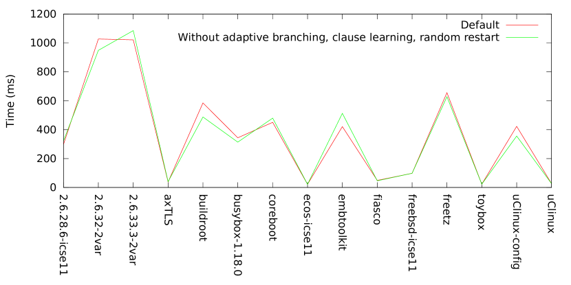
Figure 1: Solving times for real-world feature models with Sat4j.

Figure 1 shows the solving times of the real-world feature models with the Sat4j solver [14] (version 2.3.4). With the default settings, the hardest feature model took a little over a second to solve. Clearly, the size of these feature models is not a problem for Sat4j. Modern SAT solvers have (at least) 4 main features that contribute to their performance: conflict-driven clause learning with backjumping, random search restarts, Boolean constraint propagation (BCP) using lazy data structures, and conflict-based adaptive branching called VSIDS [13]. Many modern solvers also implement pre-processing simplification techniques. Sat4j implements all these features except pre-processing simplifications. Figure 1 shows the running time after turning off 3 of these features, but the running times did not suffer significantly. BCP is surprisingly effective for real-world feature models. The efficiency even without state-of-the-art techniques suggests that real-world FMs are easy to solve.

3.3 Experiment: Hard artificial FMs

The question we posed in this experiment was whether it is possible to construct hard artificial FMs, and if so what would their structural features be. Indeed, we were able to construct small feature models that are very hard for SAT solvers. The procedure we used to generate such models is as follows:

1. First, we randomly generate a small and hard CNF formula. One such method is to generate random 3-SAT with a clause density of 4.25. It is well-known that such random instances are hard for a CDCL SAT solver to solve [1]. We then used such generated problems as the cross-tree constraints for our hard FMs.

2. Second, we generate a small tree with only optional features. The variables that occur in the cross-tree constraints from the first step are the leaves of the tree.

The key idea in generating such FMs is that for any pair of variables in the cross-tree constraints, the tree does not impose any constraints between the two. The problem then is as hard as the cross-tree constraints because a solution for the feature model is a solution for the cross-tree constraints and vice-versa. Using this technique, we can create small feature models that are hard to solve. Unlike these hard artifical FMs, the cross-tree constraints in large real-world FMs are evidently easy to solve. We also noted that the proportion of unrestricted variables in hard artificial FMs is relatively small.

3.4 Experiment: Variability in real-world FMs

Feature models capture variability, and we believe that the search for valid product configuration is easier as variability increases. We hypothesized that finding a solution is easy, when the solver has numerous solutions to choose from. We ran the feature models with sharpSAT [24], a tool for counting the exact number of solutions. The results are in Table 2. We found that real-world FMs display very high variability, i.e., have lots of solutions.

Model	Variables	Solutions
axTLS	684	$2^{142}$
busybox-1.18.0	6796	$2^{720}$
coreboot	12268	$2^{313}$
ecos-icse11	1244	$2^{418}$
embtoolkit	23516	$2^{725}$
fiasco	1638	$2^{48}$
freebsd-icse11	1396	$2^{1043}$
toybox	544	$2^{57}$
uClinux-config	11254	$2^{1388}$
uClinux	1850	$2^{303}$

Table 2: The variability in real-world feature models, counted by sharpSAT. The computation finished for 10 of the 15 models.

Variability is the reason feature models exist. The feature groups and optional features increase the variability in the model, and the results in Table 2 suggests the variability grows exponentially with the size of the model measured in number of variables. High variability in real-world FMs should have structural properties that make them easy to solve.

3.5 Experiment: Why solvers perform very few backtracks for real-world FMs

The goal of this experiment was to ascertain why solvers make so few backtracks while solving real-world FMs. First, observe that when a solver needs to make new decision, it must guess the correct assignment for the decision variable-in-question under the current partial assignment in order to avoid backtracking. Also observe that if a decision variable is unrestricted then either a true or a false assignment to such a variable would lead to a satisfying assigment. In other words, a preponderance of unrestricted variable in an input formula to a solver implies that the solver will likely make few mistakes in assigning values to decision variables and thus perform very few backtracks during solving.

Given the above line of reasoning, we designed an experiment that would increase our confidence in our hypothesis that a vast majority of the variables in real-world FMs are unrestricted, and that the presence of these large number of unrestricted variables explains why SAT solvers perform very few backtracks while solving real-world FMs. The experiment is as follows: whenever the solver branches on a decision or backtracks (i.e., when the partial assignment changes), we take a snapshot of the solver’s state. We want to examine how many unassigned variables are unrestricted/restricted. This requires copying the state of the snapshot into a new solver and checking if there are indeed solutions in both assignment branches of the variable under the current partial assignment, in which case the variable-in-question is unrestricted. If only true branch (resp. false branch) has a solution, then it is a postively restricted (resp. negatively restricted) variable. If neither branch has a solution, then the current partial assignment is unsatisfiable.

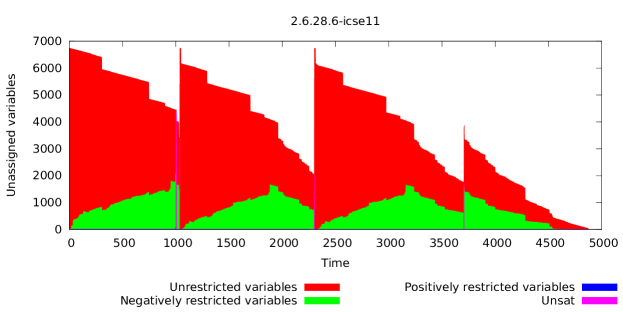
Figure 2: Unrestricted and restricted variables for a Linux-based feature model as Sat4j solves the corresponding Boolean formula. Time is measured by the number of decisions and conflicts. The y-axis shows the unassigned variables under the current partial assignment. For example, once the solver reached 500 decisions/conflicts, about 5700 of the variables were unassigned, approximately 1000 of these unassigned variables were negatively restricted variables (green) and the remainder were unrestricted variables (red). The pink area means the current partial assignment is unsatisfiable and the solver will need to backtrack eventually.

Figure 2 shows how the unrestricted variables for one Linux-based feature model change over the course of the search. The red area denotes unrestricted variables. If the solver branches on a variable in the red region, the solver will remain on the right track to finding a solution. The blue/green area denotes restricted variables. If the solver branches on a variable in the blue/green region, the solver must assign the variable the correct value.  The 15 real-world feature models have very large red regions.

A large amount of unrestricted variables suggests that the instance is easy to solve. When the decision heuristic branches on an unrestricted variable, it does not matter which branch to take, the partial assignment will remain satisfiable either way. Feature models offer enough flexibility such that the SAT solvers rarely run into dead ends.

3.6 Experiment: Simplifications

We hypothesized that since the vast majority of the variables are unrestricted they can be easily simplified away. Furthermore, the remaining variables/clauses, we call a core, would be small enough such that even a brute-force approach could solve it easily. In point of fact, most, but not all, modern solvers have both pre- and in-processing simplification techniques already built-in. The term in-processing refers to simplification techniques that are called in the inner loop of the SAT solver, whereas pre-processing techniques are typically called only once at the start of a SAT solving run.

The goal of these experiments was not to suggest a new set of techniques to analyze FMs, but rather to reinforce our findings for the effectiveness of SAT-based analysis of real-world FMs.

We implemented a number of standard simplifications that are particularly suited for eliminating variables. These simplifications were implemented as a preprocessing step to the Sat4j solver. Note that the Sat4j solver does not come packaged with variable elimination techniques, and hence we had to implement them as a pre-processor. Briefly, a simplification is a transformation on the Boolean formula where the output formula is smaller and equisatisfiable to the input formula. We carefully chose simplifications that run in time polynomial in the size of the input Boolean formula.

What we found was that indeed the simplifications were effective in eliminating more than 99% of the variables from real-world FMs. In 11 out of 15 instances from our benchmarks, the simplifications completely solved the instance without resorting to calling the backend solver. In the remaining cases, the cores were very small (at most 53 variables) and were largely Horn clauses that were easily solved by Sat4j. The simplifications we implemented are described below:

Equivalent Variable Substitution: If $x\implies y$ and $y\implies x$ where $x$ and $y$ are variables, then replace $x$ and $y$ with a fresh variable $z$. The idea behind this technique is to coalesce the variables since effectively $x=y$. This simplification step is useful for mandatory features that produce bidirectional implications in the CNF translation.

Subsumption: If $C_{1}\subset C_{2}$ where $C_{1}$ and $C_{2}$ are clauses, then $C_{2}$ is subsumed by $C_{1}$. Remove all subsumed clauses. The idea here is that subsumed clauses are trivially redundant. Initially, no clauses are subsumed in the real-world feature models. After other simplifications, some clauses will become subsumed.

Self-Subsuming Resolution: If $C\vee x$ and $C\vee\neg x\vee D$ where $C$ and $D$ are clauses and $x$ is a literal, then replace with $C\vee x$ and $C\vee D$. The idea here is that if $x=true$ then $C\vee\neg x\vee D$ reduces to $C\vee D$. If $x=false$ then $C=true$ in which case both $C\vee\neg x\vee D$ and $C\vee D$ are satisfied. In either case, $C\vee\neg x\vee D$ is equal to $C\vee D$, hence the clause can be shortened by removing the variable $x$.

Some features in the 3 Linux models are tristate: include the feature compiled statically, include the feature as a dynamically loadable module, or exclude the feature. Tristate features require two Boolean variables to encode. This simplification step is particularly useful for tristate feature models. For example, the feature $A$ is encoded using Boolean variables $a$ and $a^{\prime}$. Table 3 shows how to interpret the values of this pair of variables.

$a$	$a^{\prime}$	Meaning
$true$	$true$	Include A compiled statically
$true$	$false$	Include A as a dynamically loadable module
$false$	$false$	Exclude feature A

Table 3: Interpretation of tristate features.

To restrict the possibilities to one of these 3 combinations, the translation adds the clause $a\vee\neg a^{\prime}$. Since the interpretation of the feature requires both variables, they often appear together in clauses. Any other clause that contains $a\vee\neg a^{\prime}$ will be removed by subsumption. Any other clause that contains $a\vee a^{\prime}$ or $\neg a\vee\neg a^{\prime}$ will be shortened by self-subsuming resolution.

Variable Elimination: Let $T$ be the set of all clauses that contain a variable and its negation. Let $x$ be a variable. $S_{x}$ is the set of clauses where the variable $x$ appears only positively. $S_{\overline{x}}$ is the set of clauses where the variable $x$ appears only negatively. The variable $x$ is eliminated by replacing the clauses $S_{x}$ and $S_{\overline{x}}$ with:

$\{C_{1}\vee C_{2}\ \mid\ (x\vee C_{1})\in S_{x},\ (\neg x\vee C_{2})\in S_{\overline{x}},\ (C_{1}\vee C_{2})\notin T\}$

The idea here is to proactively apply an inference rule from propositional logic called the resolution rule. This simplification step is called variable elimination because the variable $x$ no longer appears in the resulting formula. This rule is only applied to variables where the number of output clauses is less than or equal to the number of input clauses.

This simplification step is very effective for pure literals. A variable is pure if it appears either only positively or only negatively in the input formula. If a variable is pure, then variable elimination will eliminate that variable and every clause containing that variable. 37.8% of variables in the 15 real-world feature models from Table 1 are pure. More variables can become pure as the formula is simplified.

Asymmetric Branching: For a clause $x\vee C$, where $x$ is a literal and $C$ is the remainder of the clause, temporarily add the constraint $\neg C$. If a call to BCP returns unsatisfiable, then learn the clause $C$. The new learnt clause subsumes the original clause $x\vee C$ so remove the original clause. Otherwise, no changes.

RCheck: For a clause $C$, temporarily replace the clause with the constraint $\neg C$. If a call to BCP returns unsatisfiable, then the other clauses imply $C$ so the clause is redundant. Remove $C$ from the formula. Otherwise, no changes. The idea is to remove all clauses that are implied modulo BCP. Implied clauses can be useful for a SAT solver to prune the search space, for example learnt clauses, but they complicate analysis.

BCP: The last simplification step is to apply BCP: if a clause of length $k$ has $k-1$ of its literals assigned to false, then assign the last literal to true.

3.6.1 Fixed Point

We repeat the simplifications a maximum of 5 times or stop when a fixed point is reached. The simplifications can only shorten the size of the input formula with the exception of variable elimination. It is unclear how many passes of simplification are necessary to reach a fixed point in the worst-case with variable elimination in the mix. The upper limit of 5 passes is to guarantee a polynomial (in the size of the input formula) number of passes. For the models from Table 1, 2 to 3 passes are enough to reach a fixed point using the current implementation built on top of MiniSat’s simplification routine. Each additional pass, in practice, experiences diminishing returns and 5 passes should be sufficient to simplify real-world feature models. The remaining formula after the 5 passes of simplifications is the core.

The worst-case execution time of the simplifications is polynomial in the size of the input formula. We used a standard encoding of FMs into Boolean formulas that are polynomially larger than the FMs in the number of features.

Model	Variables	Clauses	Horn (%)	Anti-Horn (%)	Binary (%)	Other (%)
2.6.28.6-icse11	30	335	93.73	6.87	93.73	0.00
2.6.32-2var	0	0	NA	NA	NA	NA
2.6.33.3-2var	0	0	NA	NA	NA	NA
axTLS	0	0	NA	NA	NA	NA
buildroot	0	0	NA	NA	NA	NA
busybox-1.18.0	0	0	NA	NA	NA	NA
coreboot	53	153	84.31	73.86	58.17	0.00
ecos-icse11	0	0	NA	NA	NA	NA
embtoolkit	20	67	82.09	22.39	17.91	0.00
fiasco	30	384	99.74	7.03	99.74	0.00
freebsd-icse11	0	0	NA	NA	NA	NA
freetz	0	0	NA	NA	NA	NA
toybox	0	0	NA	NA	NA	NA
uClinux-config	0	0	NA	NA	NA	NA
uClinux	0	0	NA	NA	NA	NA

Table 4: Clause and variable count of simplified real-world FMs. If the variable count is 0, then the simplification solved the instance because there are no variables remaining.

3.6.2 Simplified Feature Models

Table 4 shows the simplified feature models. Simplification alone is able to solve 11 of the models without resorting to a backend solver. The remaining 4 are shrunk drastically in terms of variables and clauses by simplification.

At least 80% of the clauses in the simplified models are Horn. Horn-satisfiability can be solved in polynomial time. The algorithm works by applying BCP, and the Horn-formula is unsatisfiable if and only if the empty clause is derived. A similar algorithm for anti-Horn-satisfiability also exists. BCP is the engine for solving Horn-satisfiability in polynomial time and modern SAT solvers implement BCP, hence we hypothesize that Boolean formulas with $\leq 53$ variables and $\geq 80\%$ Horn clauses are easy for SAT solvers to solve.

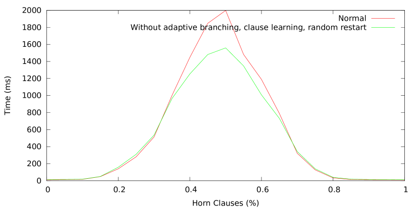
Figure 3: Solving Horn clauses for randomized 3-SAT (200 variables and 850 clauses) with Sat4j. The clause density is set to 4.25, where random 3-SAT is hardest to solve.

Figure 3 shows how Horn clauses make solving easier. Note that for 3-SAT, every clause is either Horn xor anti-Horn, hence the symmetry in the graph. Every point in the graph is the average running time of 100 randomly generated 3-SAT instances. The instances were generated with 200 variables, which is larger than the simplified coreboot model. The running times where the Horn clauses exceed 80% is very low. Clause learning, adaptive branching, and random restarts are not necessary for this case. Although we originally suspected the core might be hard for its size, the core itself turned out to be easy as well.

3.7 Experiment: Treewidth of real-world FMs

Experiments by Pohl et al. [19] show treewidth of the CNF representation of randomly-generated FMs to be strongly correlated with their corresponding solving times. We repeat the experiment on the real-world FMs to see if the correlation exists. In our experiments, treewidth is computed by finding a lower and upper bound because the exact treewidth computation is too expensive to compute. The longer the calculation runs, the tighter the bounds are. We used the same algorithm and package used by Pohl et al. We gave the algorithm a timeout of 3600 seconds and 24 GB of heap memory, up from 1000 seconds and 12 GB in the original experiment by Pohl et al. Figure 4 shows the results. The computation failed to place any upper bound on 9 FMs, and we omit these results because we do not know how close the computed lower bounds are to the exact answer. For the 6 models in the table, the lower and upper bound are close, and hence close to the exact answer.

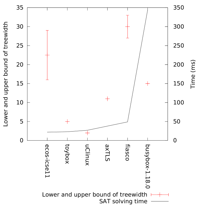
Figure 4: Treewidth of real-world FMs plotted against solving time. 4 models have exact bounds.

We used Spearman’s rank correlation, the same correlation method as in the original experiment, to correlate the lower bound and time. We found the correlation between the lower bound and time to be 0.257. We get the same number when correlating between the upper bound and time (Spearman’s rank correlation is based on the rank and the lower and upper bound rank the models in the same order). Our results show a significantly poorer correlation than previous work on randomly-generated FMs. Although our sample is small, research on treewidth in real-world SAT instances (not FMs) have also found similar results, i.e., that treewidth of input Boolean formulas is not strongly correlated with running time of solvers and is not indicative of an instance’s hardness [15].

3.8 Interpretation of Results

It is clear from our experiments that the vast majority of variables in real-world FMs are unrestricted and can be solved/analyzed by appropriate simplification and BCP in time polynomial in the number of variables of the corresponding SAT instance. What remains after BCP and simplification is a very small set of core clauses (small relative to the number of clauses in the input SAT formula) which can be solved by a CDCL solver with very few backtracks.

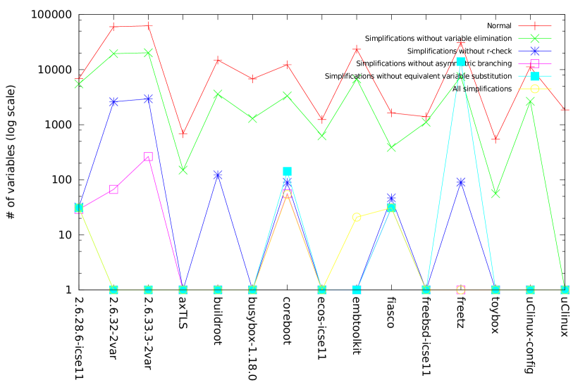
Figure 5: The effectiveness of simplifications at reducing the number of variables. We try turning off simplifications one at a time and measure the result. The line “normal" is the original input Boolean formula with no simplifications.

4 Threats to Validity of Experimental Methodology and Results

In this section, we address threats to validity of our experimental methodology and results.

Validity of FMs used for the Experiments: The studied collection of FMs are large real-world feature models [8], primarily based on software product lines. This collection includes all large real-world models that are publicly available. Further, systems software, the domain of these models, is known to produce some of the most complex configuration constraints [5]. After taking into account the complexity of these models, we believe that these findings will likely hold for many other large real-world models.

Validity of Experimental Methodology: The unrestricted variables experiment takes the partial assignments we encounter during the run of the solver with default parameters. The partial assignments could vary if the branching heuristic is initiated with a random seed. Ideally, we would like to show that unrestricted variables are plentiful under any partial assignment but this would require an infeasible amount of effort to prove. Having said that, there is no reason to believe that the number of unrestricted variables would change drastically for a different random seed. In fact, once we realized that real-world FMs have large number of unrestricted variables, we were able to analytically show that these unrestricted variables occur in such formulas due to the high variability of FMs. This high variability in FMs is a fundamental property of such models, and is independent of translation to SAT or random seed chosen.

Correctness of Mapping of FMs into SAT: The analyses rely on the correctness of mapping of the Kconfig and CDL models to propositional logic. We rely on existing work that reverse engineered the semantics of these languages from documentation and configuration tools and specified the semantics formally [7, 8].

Validity of Choice of Solvers: All our experiments were performed using the Sat4j solver [14]. An important concern is whether these results would apply to other SAT solvers and analysis tools built using them. Our choice of Sat4j was driven by the fact that it is one of the simplest CDCL SAT solver publicly available, and this simplicity makes it easier to draw correct conclusions. Note that most other SAT solvers used in FM analysis are not only CDCL in the same vein as Sat4j, but also implement efficient variants of simplification techniques discussed above. Hence, we believe that our results would apply equally well to other solvers used in FM analysis. Finally, we did not consider CSP or BDD-based solvers since CDCL solvers are demonstrably better for FM analysis based on the standard encoding used by Benavides et al. [4].

5 Related Work

Using constraint solvers to analyze feature models has a long tradition. Benavides et al. [3] give a comprehensive survey of techniques for analyzing feature models, such as checking consistency and detecting dead features, and for supporting configuration, such as propagating feature selections. These techniques use a range of solvers, including SAT and CSP solvers. Batory [2] was first to suggest the use of SAT solvers to support feature model analyses.

Several authors have investigated the efficiency of different kinds of solvers for feature model analyses. Benavides et al. [4] compare the performance of SAT, CSP, and BDD solvers on two sample analyses on randomly generate feature models with up to 300 features. They show that BDD solvers are prone to exponential growth in memory usage on larger models, while SAT solvers achieve good runtime performance in the experiments. Pohl et al. [18] run similar comparison on feature models from the SPLOT collection, including a wider set of solver implementations. SPLOT models are relatively small—the largest one has less than 300 features—and are derived from academic works. Their results show that SAT solvers work well also for SPLOT models, although they detect some performance variation for C- vs. Java-based SAT solvers; they also confirm the tractability challenges for BDD solvers. Mendonca et al. [17] achieve scalability of BDD-based analyses to randomly generated feature models with up to 2000 features by optimizing the translation from the models to BDDs using variable ordering heuristics based on the feature hierarchy. Further, Mendonca et al. [16] show that SAT-based analyses scale to randomly generated feature models with up to 10000 features. All this previous work shows that SAT solvers perform well on small realistic feature models (SPLOT collection) and large randomly generated feature models. Although SAT solvers have been successfully applied to analyze the feature model of the Linux kernel [22], we are unaware of prior work systematically studying the performance of SAT solvers on large (1000+ features) real-world feature models, which is what we focus on in this paper.

Previous work has also investigated the hardness of the SAT instances derived from feature models, aiming at more general insights into the tractability of SAT-based analyses. Mendonca et al. [16] have studied the SAT solving behavior of randomly generated 3-SAT feature models. A 3-SAT feature model is one whose cross-tree constraints are 3-SAT formulas. While random 3-SAT formulas become hard when their clause density approaches 4.25 (so-called phase transition), this work shows experimentally that 3-SAT feature models remain easy across all clause densities of their corresponding 3-SAT formulas. Our work is different since it investigates the hardness of large real-world feature models rather than random ones. Even though random feature models are easy on average, specific instances may still be hard; for example, a tree of optional features with a hard 3-SAT cross-tree formula over the tree leaves is, albeit contrived, a hard feature model. Segura et al. [20] treat finding hard feature models as an optimization problem. They apply evolutionary algorithms to generate feature models of a given size that maximize solving time or memory use. Their experiments show that relatively small feature models can become intractable in terms of memory use for BDDs; however, the approach did not generate feature models that would be hard for SAT solvers. Again, this work only considers synthetically generated feature models, rather than real-world ones.

Finally, Pohl et al. [19] propose graph width measures, such as treewidth, applied to graph representations of the CNF derived from a feature model as a upper bound of the complexity of analyses on the model. Their work evaluates this idea on a set of randomly generated feature models with up to 1000 features using SAT, CSP, and BDD solvers; they also repeat the experiment on the SPLOT collection. They find a significant correlation between certain treewidth measures on the incidence graph and the running time for most of the solvers. Further, the authors note that it is still unclear why SPLOT models are easier than generated ones, and whether that observation would hold for large-scale real-world feature models. Our work addresses this gap by investigating the hardness of large-scale real-world feature models and providing an explanation why they are easy. Moreover, we were not able to identify any correlation between the treewidth and easiness of the SAT instances derived from large real-world models, which calls for more work to find effective hardness measures for feature models.

Large real-world models have become available to researchers only recently. While some papers hint at the existence of very large models in industry [6], these models are typically highly confidential. Sincero [21] was first to observe that the definition of the Linux kernel build configuration, expressed in the Kconfig language, can be viewed as a feature model. Berger et al. [7] identify the Component Definition Language (CDL) in eCos, an open-source real-time operating system, as additional feature modeling language and subsequently [8] create and analyze a collection of large real-world feature models from twelve open-source projects in the software systems domain. We use this collection as a basis for our work.

6 Conclusions

In this paper, we provided an explanation, with strong experimental support, for the scalability of SAT solvers on large real-world FMs. The explanation is that the overwhelming majority of the variables in real-world FMs are unrestricted, and solvers tend not to backtrack in the presence of such variables. We argue that the reason for the presence of large number of unrestricted variables in real-world FMs has to do with high variability in such models. We also found that if we switch off all the heuristics in modern SAT solvers, except Boolean constraint propagation (BCP) and backjumping (no clause-learning), then the solver does not suffer any deterioration in performance while solving FMs. Moreover, we ran a set of simplifications with substantial reduction to the size of the instances. In fact, a majority of the models were solved outright with these polynomial-time simplifications. These experiment further bolster our thesis that most variables in real-world FMs are unrestriced that can be eliminated by BCP or appropriate simplifications, and do not cause SAT solvers to perform expensive backtracks. Finally, we note that variables/clauses that are not eliminated through BCP or simplification, namely the core, are so few and mostly Horn that backtracking solvers can easily solve them.

Visit the following URL to download further details of the experiments we performed and additional associated data:
https://github.com/JLiangWaterloo/fmeasy.

References

- [1] A. Balint, A. Belov, M. Järvisalo, and C. Sinz. Overview and analysis of the SAT Challenge 2012 solver competition. Artificial Intelligence, 223:120–155, 2015.
- [2] D. Batory. Feature models, grammars, and propositional formulas. In Proceedings of the 9th International Conference on Software Product Lines, SPLC’05, pages 7–20, Berlin, Heidelberg, 2005. Springer-Verlag.
- [3] D. Benavides, S. Segura, and A. Ruiz-Cortés. Automated analysis of feature models 20 years later: A literature review. Information Systems, 35(6):615 – 636, 2010.
- [4] D. Benavides, S. Segura, P. Trinidad, and A. Ruiz-Cortés. A first step towards a framework for the automated analysis of feature models. In Managing Variability for Software Product Lines: Working With Variability Mechanisms, 2006.
- [5] T. Berger, R.-H. Pfeiffer, R. Tartler, S. Dienst, K. Czarnecki, A. Wasowski, and S. She. Variability mechanisms in software ecosystems. Information and Software Technology, 56(11):1520–1535, 2014.
- [6] T. Berger, R. Rublack, D. Nair, J. M. Atlee, M. Becker, K. Czarnecki, and A. Wasowski. A survey of variability modeling in industrial practice. In Proceedings of the Seventh International Workshop on Variability Modelling of Software-intensive Systems, VaMoS ’13, pages 7:1–7:8, New York, NY, USA, 2013. ACM.
- [7] T. Berger, S. She, R. Lotufo, A. Wasowski, and K. Czarnecki. Variability modeling in the real: A perspective from the operating systems domain. In Proceedings of the IEEE/ACM International Conference on Automated Software Engineering, ASE ’10, pages 73–82, New York, NY, USA, 2010. ACM.
- [8] T. Berger, S. She, R. Lotufo, A. Wasowski, and K. Czarnecki. A study of variability models and languages in the systems software domain. IEEE Trans. Softw. Eng., 39(12):1611–1640, Dec. 2013.
- [9] K. Czarnecki and U. W. Eisenecker. Generative Programming: Methods, Tools, and Applications. ACM Press/Addison-Wesley Publishing Co., New York, NY, USA, 2000.
- [10] R. Gheyi, T. Massoni, and P. Borba. A theory for feature models in Alloy. pages 71–80, Portland, USA, November 2006.
- [11] M. Janota. Do SAT solvers make good configurators? In SPLC (2), pages 191–195, 2008.
- [12] K. C. Kang, S. G. Cohen, J. A. Hess, W. E. Novak, and A. S. Peterson. Feature-oriented domain analysis (FODA) feasibility study. Technical report, Carnegie-Mellon University Software Engineering Institute, November 1990.
- [13] H. Katebi, K. A. Sakallah, and J. a. P. Marques-Silva. Empirical study of the anatomy of modern SAT solvers. In Proceedings of the 14th International Conference on Theory and Application of Satisfiability Testing, SAT’11, pages 343–356, Berlin, Heidelberg, 2011. Springer-Verlag.
- [14] D. Le Berre, A. Parrain, M. Baron, J. Bourgeois, Y. Irrilo, F. Fontaine, F. Laihem, O. Roussel, and L. Sais. Sat4j-a satisfiability library for java, 2006.
- [15] R. Mateescu. Treewidth in industrial SAT benchmarks. Technical report, Microsoft Research, 2011.
- [16] M. Mendonca, A. Wasowski, and K. Czarnecki. SAT-based analysis of feature models is easy. In Proceedings of the 13th International Software Product Line Conference, SPLC ’09, pages 231–240, Pittsburgh, PA, USA, 2009. Carnegie Mellon University.
- [17] M. Mendonca, A. Wasowski, K. Czarnecki, and D. Cowan. Efficient compilation techniques for large scale feature models. In Proceedings of the 7th International Conference on Generative Programming and Component Engineering, GPCE ’08, pages 13–22, New York, NY, USA, 2008. ACM.
- [18] R. Pohl, K. Lauenroth, and K. Pohl. A performance comparison of contemporary algorithmic approaches for automated analysis operations on feature models. In Proceedings of the 2011 26th IEEE/ACM International Conference on Automated Software Engineering, ASE ’11, pages 313–322, Washington, DC, USA, 2011. IEEE Computer Society.
- [19] R. Pohl, V. Stricker, and K. Pohl. Measuring the structural complexity of feature models. In Automated Software Engineering (ASE), 2013 IEEE/ACM 28th International Conference on, pages 454–464, Nov 2013.
- [20] S. Segura, J. A. Parejo, R. M. Hierons, D. Benavides, and A. R. Cortés. Automated generation of computationally hard feature models using evolutionary algorithms. Expert Syst. Appl., 41(8):3975–3992, 2014.
- [21] J. Sincero, H. Schirmeier, W. Schröder-Preikschat, and O. Spinczyk. Is the linux kernel a software product line. In Proc. SPLC Workshop on Open Source Software and Product Lines, 2007.
- [22] R. Tartler, D. Lohmann, J. Sincero, and W. Schröder-Preikschat. Feature consistency in compile-time-configurable system software: Facing the linux 10,000 feature problem. In Proceedings of the Sixth Conference on Computer Systems, EuroSys ’11, pages 47–60, New York, NY, USA, 2011. ACM.
- [23] T. Thum, D. Batory, and C. Kastner. Reasoning about edits to feature models. In Proceedings of the 31st International Conference on Software Engineering, ICSE ’09, pages 254–264, Washington, DC, USA, 2009. IEEE Computer Society.
- [24] M. Thurley. sharpsat: Counting models with advanced component caching and implicit BCP. In Proceedings of the 9th International Conference on Theory and Applications of Satisfiability Testing, SAT’06, pages 424–429, Berlin, Heidelberg, 2006. Springer-Verlag.