Non-equilibrium interfacial tension during relaxation

Abstract

The concept of a non-equilibrium interfacial tension, defined via the work required to deform the system such that the interfacial area is changed while the volume is conserved, is investigated theoretically in the context of the relaxation of an initial perturbation of a colloidal fluid towards the equilibrium state. The corresponding general formalism is derived for systems with planar symmetry and applied to fluid models of colloidal suspensions and polymer solutions. It is shown that the non-equilibrium interfacial tension is not necessarily positive, that negative non-equilibrium interfacial tensions are consistent with strictly positive equilibrium interfacial tensions, and that the sign of the interfacial tension can influence the morphology of density perturbations during relaxation.

I Introduction

The equilibrium interfacial tension between two coexisting fluid phases is a well established concept of enormous relevance to numerous research areas such as capillarity, wetting, the morphology of drops and bubbles, interface dynamics, and the adsorption of surfactant molecules or colloidal particles at interfaces Safran2003 ; deGennes2004 . It is well-known that the equilibrium interfacial tension can be equivalently viewed either mechanically in terms of the difference of the normal and the transversal pressure tensor components or thermodynamically via the work required to reversibly deform the system in such a way that the interfacial area is changed while the system volume is preserved Rowlinson2002 . Both interpretations require the notion of the position of the interface, i.e., of the non-uniform part of the system, which can be defined via the concept of a Gibbs dividing interface Rowlinson2002 . However, it can be shown that the value of the equilibrium interfacial tension between two fluid phases is independent of the choice of the Gibbs dividing interface Rowlinson2002 .

In contrast, the general concept of an interfacial tension in non-equilibrium situations, e.g., a non-equilibrium interface between two coexisting equilibrium bulk phases or an interface between two bulk phases being not at coexistence with each other, has not been uniquely established yet. Several attempts have been made to extend the notion of an interfacial tension to non-equilibrium systems in order to interpret dynamic phenomena at interfaces Joos1999 ; Drelich2006 . The approaches range from time-resolved interfacial tension measurements Peach1996 via integrations of the Gibbs equation Maze1971 ; Adamczyk1987 ; Millner1994 ; Eastoe2000 to capillary wave analyses Cicuta2000 . The overall assumption underlying all these non-equilibrium interfacial tensions is that of a sufficiently weakly perturbed equilibrium interface. In fact, it has been shown recently that the interfacial structure between two fluid bulk phases not in thermodynamic equilibrium with each other converges rapidly towards that of the equilibrium interface between the two coexisting bulk phases at the same temperature Bier2013 . Hence, different notions of dynamic interfacial tensions can be expected to coincide quantitatively provided they do so for equilibrium interfaces. However, unlike for equilibrium interfaces, the value of the non-equilibrium interfacial tension depends on the choice of the Gibbs dividing interface Levitas2014 .

It is well-known that the interfacial tension of equilibrium fluid-fluid interfaces is strictly positive because otherwise the interface would be unstable with respect to capillary wave fluctuations. The aim of the present work is to demonstrate that this is not necessarily the case for non-equilibrium interfacial tensions. To that end, the relaxation of an initial non-uniformity of a fluid deep inside the one-phase region of the phase diagram is considered. Under these conditions the equilibrium state is uniform, i.e., no equilibrium interface exists. Therefore, the initial non-uniformity, i.e., the interface, is a purely non-equilibrium structure, which ultimately vanishes during relaxation towards equilibrium.

The present analysis is based on the notion of a non-equilibrium interfacial tension similar to the thermodynamic definition related to the work of reversible isochoric deformations. It has been shown in Ref. Bier2013 that this notion of a non-equilibrium interfacial tension is not only consistent with the equilibrium interfacial tension but also useful in the context of interfaces between phases separated by a fluid-fluid phase transition. In order to avoid the difficulty due to the dependence of the non-equilibrium interfacial tension on the choice of the Gibbs dividing interface, setups are considered for which the cross-sections of the system perpendicular to one spatial direction ($z$-axis) are all congruent. For such setups the number density profiles of the fluid vary only along the $z$-axis and the interfacial area equals the area of any of the congruent cross-sections. Then locating the interface position is not necessary.

In order to apply the definition of the non-equilibrium interfacial tension as the work due to a reversible isochoric deformation in practice, the deformation has to be performed faster than the relaxation of the fluid under consideration. However, this is not possible in practice for simple fluids, since deformations have to be induced by deformations of the container walls, from where they propagate into the fluid via particle-particle interactions. Hence reversible deformations of a simple fluid cannot be achieved on time scales faster than the relaxations.

One way out of this dilemma is to consider fluids of colloidal particles which are dispersed in a molecular solvent. In that situation, deformations of the container walls induce deformations of the molecular solvent which propagate on time scales much shorter than the relaxation time of the colloids. Hence the solvent is the tool that exerts the force generated by the container walls onto the colloidal particles, which are considered as the fluid to be studied.

The general formalism used in this work is derived in Sec. II. First some notation to model colloidal suspensions are introduced in Sec. II.1. The non-equilibrium properties as well as the interfacial structures of colloidal fluids can be described simultaneously within dynamic density functional theory (DDFT) Evans1979 ; Dieterich1990 ; Kawasaki1994 ; Dean1996 ; MariniBettoloMarconi1999 ; MariniBettoloMarconi2000 , the relevant concepts of which are summarized in Sec. II.2. The expression of the interfacial tension as a functional of the interfacial density profile is derived in detail in Sec. II.3. The evaluation of the interfacial tension for temporally evolving density profiles obtained within DDFT leads to the time-dependence of the interfacial tension in Sec. II.4. The the application of the general formalism of Sec. II is illustrated in Sec. III for three realistic fluid models, all of which exhibit negative values of the non-equilibrium interfacial tension. Conclusions from the possibility of negative non-equilibrium interfacial tensions and the property of strictly positive equilibrium interfacial tensions are drawn in Sec. IV.

II General formalism

II.1 Colloidal suspensions

Consider a three-dimensional monodisperse suspension of colloidal particles which interact amongst each other via an isotropic pair potential $U(r),r=|\mathbf{r}_{1}-\mathbf{r}_{2}|$. The temperature $T$ and the mean number density $\bar{\varrho}$ of colloidal particles are chosen such that in the absence of an external field the equilibrium state of the system is that of a uniform isotropic fluid well inside a one-phase region of the phase diagram.

The fluid structure of that uniform equilibrium state is given by the isotropic direct correlation function $\bar{c}(r):=c(r,\bar{\varrho}),r=|\mathbf{r}_{1}-\mathbf{r}_{2}|$. It can be shown very generally that if $U(r)$ decays to zero for $r\to\infty$ faster than some power law $\sim r^{-s},s>5$, i.e., if there exists some $s>5$ with $\displaystyle\lim_{r\to\infty}r^{s}U(r)=0$, the three-dimensional Fourier transform of $\bar{c}(r)$ is given by

$$\widehat{\bar{c}}(q)=\widehat{\bar{c}}_{0}+\widehat{\bar{c}}_{2}q^{2}+\mathcal{R}(q)$$ (1)

with $q=|\mathbf{q}|$ and with $\mathcal{R}(q)$ decaying to zero for $q\to 0$ faster than $q^{2}$; the derivative $\mathcal{R}^{\prime}(q)$ of $\mathcal{R}(q)$ with respect to $q$ turns out to decay to zero for $q\to 0$ faster than $q$. The situation just described covers practically all cases of isotropically interacting colloids, e.g., non-retarded dispersion forces in dense suspensions, retarded dispersion forces in dilute suspensions, orientationally averaged magnetic dipole interaction, as well as pure screened Coulomb interaction for suspensions with the index of refraction of the solvent being matched to that of the colloids.

At time $t<0$ a static external field is applied to the colloidal suspension giving rise to a non-uniform equilibrium number density profile $\varrho_{0}(\mathbf{r})$ with mean number density $\displaystyle\bar{\varrho}=\frac{1}{|V|}\int_{V}\!\mathrm{d}^{3}r\,\varrho_{0}(\mathbf{r})$. At time $t=0$ the external field is switched off leaving the colloidal suspension in a non-equilibrium state, which relaxes for $t\to\infty$ towards the equilibrium state with the uniform number density $\bar{\varrho}$. In the following the temporal evolution of the non-equilibrium state of the colloidal suspension is investigated in terms of the time-dependent number density profile $\varrho(\mathbf{r},t)$, which at time $t=0$ is given by $\varrho(\mathbf{r},0)=\varrho_{0}(\mathbf{r})$ and which attains the long time limit $\displaystyle\lim_{t\to\infty}\varrho(\mathbf{r},t)=\bar{\varrho}$. The deviation of the number density $\varrho(\mathbf{r},t)$ from its long time limit $\bar{\varrho}$ is denoted as $\phi(\mathbf{r},t):=\varrho(\mathbf{r},t)-\bar{\varrho}$, which decays to zero in the long time limit: $\displaystyle\lim_{t\to\infty}\phi(\mathbf{r},t)=0$.

II.2 Dynamic density functional theory

The relaxation of colloidal suspensions can be described as an overdamped conserved dynamics (model B), which can be formulated in terms of dynamic density functional theory Dieterich1990 . If the system is prepared in an arbitrary initial state $\varrho(\mathbf{r},t=0)$, its state $\varrho(\mathbf{r},t>0)$ evolves with time $t$ such that the Helmholtz free energy $F[\varrho(t)]$ reaches a minimum at $t\to\infty$.

The Helmholtz free energy density functional $F[\varrho]$ can be written as

$$\beta F[\varrho]=\int\!\mathrm{d}^{3}r\,\varrho(\mathbf{r})\left(\ln(\varrho(\mathbf{r})\Lambda^{3})-1\right)+\beta F^{\text{ex}}[\varrho-\bar{\varrho}]$$ (2)

with the inverse temperature $\beta=1/(k_{\text{B}}T)$. The excess free energy functional $\beta F^{\text{ex}}[\phi]$ can be expanded in a functional Taylor series in powers of $\phi=\varrho-\bar{\varrho}$, which results in the virial expansion

$$\beta F^{\text{ex}}[\phi]= \beta F^{\text{ex}}[0]-c^{(1)}(\bar{\varrho})\int\!\mathrm{d}^{3}r\,\phi(\mathbf{r})$$

$$-\frac{1}{2}\int\!\mathrm{d}^{3}r\!\int\!\mathrm{d}^{3}r^{\prime}\,c^{(2)}(|\mathbf{r}-\mathbf{r^{\prime}}|,\bar{\varrho})\phi(\mathbf{r})\phi(\mathbf{r^{\prime}})$$

$$+\mathcal{O}(\phi^{3}).$$ (3)

The term linear in $\phi$ drops out because $\displaystyle\int\mathrm{d}^{3}r\,\phi(\mathbf{r})=0$, and $c^{(2)}(r,\bar{\varrho})=c(r,\bar{\varrho})=\bar{c}(r)$. Since $\phi(\mathbf{r},t)\to 0$ for $t\to\infty$, the approximation

$$\beta F^{\text{ex}}[\phi]\simeq\ \beta F^{\text{ex}}[0]$$

$$-\frac{1}{2}\int\!\mathrm{d}^{3}r\!\int\!\mathrm{d}^{3}r^{\prime}\,\bar{c}(|\mathbf{r}-\mathbf{r^{\prime}}|)\phi(\mathbf{r})\phi(\mathbf{r^{\prime}})$$ (4)

is applicable, at least at sufficiently late times $t$.

Since the colloidal processes considered in the present work, which are described in terms of $\varrho(\mathbf{r},t)$, are much slower than the molecular degrees of freedom, one can assume local thermodynamic equilibrium and define the local chemical potential Dieterich1990

$$\beta\mu(\mathbf{r},[\varrho(t)]) =\frac{\delta\beta F}{\delta\varrho(\mathbf{r})}[\varrho(t)]$$

$$=\ln(\varrho(\mathbf{r},t)\Lambda^{3})+\beta\mu^{\text{ex}}(\mathbf{r},[\phi(t)])$$ (5)

with

$$\beta\mu^{\text{ex}}(\mathbf{r},[\phi(t)]) =\frac{\delta\beta F^{\text{ex}}}{\delta\phi(\mathbf{r})}[\phi(t)]$$

$$\simeq-\int\!\mathrm{d}^{3}r^{\prime}\,\bar{c}(|\mathbf{r}-\mathbf{r^{\prime}}|)\phi(\mathbf{r^{\prime}},t).$$ (6)

The local force $-\nabla\mu(\mathbf{r},[\varrho(t)])$ generates a flux Dieterich1990

$$\mathbf{j}(\mathbf{r},[\varrho(t)]) =\beta D\left(-\nabla\mu(\mathbf{r},[\varrho(t)])\right)\varrho(\mathbf{r},t)$$

$$=-D\left(\frac{\nabla\varrho(\mathbf{r},t)}{\varrho(\mathbf{r},t)}+\nabla\beta\mu^{\text{ex}}(\mathbf{r},[\phi(t)])\right)\varrho(\mathbf{r},t)$$

$$=-D\big{(}\underbrace{\nabla\varrho(\mathbf{r},t)}_{=\nabla\phi(\mathbf{r},t)}+\bar{\varrho}\nabla\beta\mu^{\text{ex}}(\mathbf{r},[\phi(t)])\big{)}+\mathcal{O}(\phi^{2})$$

$$\simeq-D\left(\nabla\phi(\mathbf{r},t)+\bar{\varrho}\nabla\beta\mu^{\text{ex}}(\mathbf{r},[\phi(t)])\right)$$ (7)

with the diffusion constant $D$. From the continuity equation of the particle number,

$$\frac{\partial\varrho(\mathbf{r},t)}{\partial t}=-\nabla\cdot\mathbf{j}(\mathbf{r},[\varrho(t)]),$$ (8)

one obtains the conserved dynamics (model B Hohenberg1977 ) equation of motion of $\phi(\mathbf{r},t)$:

$$\frac{\partial\phi(\mathbf{r},t)}{\partial t}\simeq D\left(\nabla^{2}\phi(\mathbf{r},t)+\bar{\varrho}\nabla^{2}\beta\mu^{\text{ex}}(\mathbf{r},[\phi(t)])\right).$$ (9)

For the sake of simplicity only planar density profiles $\varrho(\mathbf{r},t)=\varrho(z,t)$, and hence $\phi(\mathbf{r},t)=\phi(z,t)$, are considered in the following. Writing

$$\phi(z,t)=:\frac{1}{2\pi}\int\!\mathrm{d}q_{z}\,\widehat{\phi}(q_{z},t)\exp(iq_{z}z)$$ (10)

one obtains from Eq. (6)

$$\beta\mu^{\text{ex}}(z,[\phi(t)])\simeq-\frac{1}{2\pi}\int\!\mathrm{d}q_{z}\,\widehat{\bar{c}}(|q_{z}|)\widehat{\phi}(q_{z},t)\exp(iq_{z}z)$$ (11)

with $\widehat{\bar{c}}(q),q=|\mathbf{q}|,$ denoting the three-dimensional Fourier-transform of $\bar{c}(r),r=|\mathbf{r}|,$ (see Eq. (1)). Hence, the equation of motion Eq. (9) for $\widehat{\phi}(q_{z},t)$ reads

$$\frac{\partial\widehat{\phi}(q_{z},t)}{\partial t}\simeq-Dq_{z}^{2}\left(1-\bar{\varrho}\,\widehat{\bar{c}}(|q_{z}|)\right)\widehat{\phi}(q_{z},t),$$ (12)

which is readily solved by

$$\widehat{\phi}(q_{z},t) =\widehat{\phi}(q_{z},0)\exp\left(-Dq_{z}^{2}t(1-\bar{\varrho}\,\widehat{\bar{c}}(|q_{z}|))\right)$$

$$=\widehat{\phi}(q_{z},0)\exp\left(-\frac{Dq_{z}^{2}t}{S(|q_{z}|)}\right),$$ (13)

where

$$S(q)=\frac{1}{1-\bar{\varrho}\,\widehat{\bar{c}}(q)}$$ (14)

is the colloidal structure factor of the uniform suspension. Equation (13) expresses the relaxation of the Fourier mode $\widehat{\phi}(q_{z},t)$ towards zero on the $q_{z}$-dependent time scale

$$\tau(|q_{z}|):=\frac{S(|q_{z}|)}{Dq_{z}^{2}}.$$ (15)

II.3 Interfacial tension

Consider a system with density profiles $\varrho(\mathbf{r},t)=\varrho(z,t)$, i.e., $\phi(\mathbf{r},t)=\phi(z,t)$, inside a container with all cross-sections perpendicular to the $z$-axis being congruent of area $A$. The interfacial tension is defined via the work which is required to change the interfacial area $A$ at constant temperature, volume, and particle number Rowlinson2002 . In colloidal suspensions such a change of the interfacial area can be achieved by deforming the incompressible molecular solvent, which drags the colloidal particles with it. Due to the separation of molecular and colloidal time scales, one is able to perform this deformation, on the one hand, sufficiently slowly in order to stay in the regime of low Reynolds numbers to avoid dissipation due to turbulence, and, on the other hand, sufficiently fast such that the colloidal distribution $\varrho(z,t)$ is practically not evolving during the measurement.

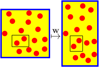
Figure 1: Sketch of the effect of the displacement field $\mathbf{w}(\mathbf{r})$ of the molecular solvent induced by a deformation of the container walls. Dispersed colloidal particles are dragged along with the solvent so that the volume as well as the number of contained colloids is conserved for each fluid element (small black frame).

By slowly deforming the boundaries of the container in a time intervall of length $t_{\text{deform}}$, a flow field $\mathbf{v}(\mathbf{r},t)$ of the solvent is induced, which fulfills the Stokes equation within the regime of low Reynolds numbers. Here $t_{\text{deform}}$ has to be long compared to the relaxation time of the molecular solvent (typically nanoseconds) and short compared to the relaxation time of the colloids (at least milliseconds). Moreover, if the velocity of the container walls is negligible compared to the sound velocity of the solvent, no pressure gradients occur inside the solvent so that the Stokes equation reduces to the Laplace equation $\nabla^{2}\mathbf{v}(\mathbf{r},t)=0$. Complementary to the Eulerian description of the flow in terms of the velocity $\mathbf{v}(\mathbf{r},t)$ at position $\mathbf{r}$ and time $t$ one can use the Lagrangian description in terms of the displacement $\mathbf{W}(\mathbf{r},t)$ within the time interval $t$ of a fluid element originally located at position $\mathbf{r}$, where both descriptions are related by

$$\frac{\partial\mathbf{W}}{\partial t}(\mathbf{r},t)=\mathbf{v}(\mathbf{r}+\mathbf{W}(\mathbf{r},t),t),\quad\mathbf{W}(\mathbf{r},0)=0.$$ (16)

From $\mathbf{W}(\mathbf{r},t)$ one obtains the displacement field $\mathbf{w}(\mathbf{r}):=\mathbf{W}(\mathbf{r},t_{\text{deform}})$ experienced by fluid elements during the time $t_{\text{deform}}$. This displacement field $\mathbf{w}(\mathbf{r})$ corresponds to the deformation map $\mathbf{r}\mapsto\mathbf{r}_{\mathbf{w}}:=\mathbf{r}+\mathbf{w}(\mathbf{r})$ of the three-dimensional space (see Fig. 1). It is assumed that the container is much larger than the colloidal particles so that $\mathbf{w}(\mathbf{r})$ is slowly varying on colloidal length scales. Due to the incompressibility of the solvent, i.e., $\nabla\cdot\mathbf{v}(\mathbf{r},t)=0$,

$$\nabla\cdot\mathbf{w}(\mathbf{r})=\mathcal{O}(\|\mathbf{w}\|^{2})$$ (17)

holds for small deformations $\|\mathbf{w}\|\to 0$. Since the considered deformations conserve the volume as well as the number of colloidal particles of the fluid elements (see Fig. 1), the number densities are not changed by the deformation map: $\varrho_{\mathbf{w}}(\mathbf{r}_{\mathbf{w}})=\varrho(\mathbf{r})$.

Upon deformation of $\phi(\mathbf{r})=\varrho(\mathbf{r})-\bar{\varrho}$ with the displacement field $\mathbf{w}(\mathbf{r})$, the excess free energy in Eq. (4) leads to

$$\beta F^{\text{ex}}[\phi_{\mathbf{w}}]-\beta F^{\text{ex}}[0]$$

$$\simeq-\frac{1}{2}\int\!\mathrm{d}^{3}r_{\mathbf{w}}\!\int\!\mathrm{d}^{3}r^{\prime}_{\mathbf{w}}\,\bar{c}(|\mathbf{r}_{\mathbf{w}}-\mathbf{r^{\prime}}_{\mathbf{w}}|)\phi_{\mathbf{w}}(\mathbf{r}_{\mathbf{w}})\phi_{\mathbf{w}}(\mathbf{r^{\prime}}_{\mathbf{w}})$$

$$=-\frac{1}{2}\int\!\mathrm{d}^{3}r\!\int\!\mathrm{d}^{3}r^{\prime}\,\bar{c}(|\mathbf{r}-\mathbf{r^{\prime}}+\mathbf{w}(\mathbf{r})-\mathbf{w}(\mathbf{r^{\prime}})|)\phi(\mathbf{r})\phi(\mathbf{r^{\prime}}).$$ (18)

Writing $c^{(2)}(\mathbf{r}):=\bar{c}(|\mathbf{r}|)$, the direct correlation function in Eq. (18) can be expanded for small deformations:

$$c^{(2)}(\mathbf{r}-\mathbf{r^{\prime}}+\mathbf{w}(\mathbf{r})-\mathbf{w}(\mathbf{r^{\prime}}))=c^{(2)}(\mathbf{r}-\mathbf{r^{\prime}})\\ +(w_{k}(\mathbf{r})-w_{k}(\mathbf{r^{\prime}}))\frac{\partial c^{(2)}}{\partial r_{k}}(\mathbf{r}-\mathbf{r^{\prime}})+\mathcal{O}(\|\mathbf{w}\|^{2}),$$ (19)

where an implicit summation over the vector components $k\in\{x,y,z\}$ is performed. Since $\displaystyle\frac{\partial c^{(2)}}{\partial r_{k}}(\mathbf{r}-\mathbf{r^{\prime}})$ vanishes for distances $|\mathbf{r}-\mathbf{r^{\prime}}|$ large compared to colloidal length scales whereas $\mathbf{w}(\mathbf{r})$ varies smoothly on colloidal length scales, the term $w_{k}(\mathbf{r})-w_{k}(\mathbf{r^{\prime}})$ in Eq. (19) can be approximated by

$$w_{k}(\mathbf{r})-w_{k}(\mathbf{r^{\prime}})\approx(r_{\ell}-r^{\prime}_{\ell})\frac{\partial w_{k}}{\partial r_{\ell}}\left(\frac{\mathbf{r}+\mathbf{r^{\prime}}}{2}\right)$$ (20)

with $\ell\in\{x,y,z\}$. Therefore Eq. (19) can be rewritten as

$$c^{(2)}(\mathbf{r}-\mathbf{r^{\prime}}+\mathbf{w}(\mathbf{r})-\mathbf{w}(\mathbf{r^{\prime}}))=c^{(2)}(\mathbf{r}-\mathbf{r^{\prime}})\\ +B_{k\ell}\left(\frac{\mathbf{r}+\mathbf{r^{\prime}}}{2}\right)\frac{\partial c^{(2)}}{\partial r_{k}}(\mathbf{r}-\mathbf{r^{\prime}})(r_{\ell}-r^{\prime}_{\ell})+\mathcal{O}(\|\mathbf{w}\|^{2}),$$ (21)

where the gradient

$$B_{k\ell}(\mathbf{r}):=\frac{\partial w_{k}}{\partial r_{\ell}}(\mathbf{r})$$ (22)

has been introduced. Using the relation

$$i(r_{\ell}-r^{\prime}_{\ell})\exp(i\mathbf{q}\cdot(\mathbf{r}-\mathbf{r^{\prime}}))=\frac{\partial}{\partial q_{\ell}}\exp(i\mathbf{q}\cdot(\mathbf{r}-\mathbf{r^{\prime}}))$$ (23)

an integration by parts leads to

$$\frac{\partial c^{(2)}}{\partial r_{k}}(\mathbf{r}-\mathbf{r^{\prime}})(r_{\ell}-r^{\prime}_{\ell})$$

$$=\int\!\!\frac{\mathrm{d}^{3}q}{(2\pi)^{3}}\,iq_{k}\widehat{\bar{c}}(|\mathbf{q}|)(r_{\ell}-r^{\prime}_{\ell})\exp(i\mathbf{q}\cdot(\mathbf{r}-\mathbf{r^{\prime}}))$$

$$=-\!\!\int\!\!\frac{\mathrm{d}^{3}q}{(2\pi)^{3}}\,\frac{\partial}{\partial q_{\ell}}\left(q_{k}\widehat{\bar{c}}(|\mathbf{q}|)\right)\exp(i\mathbf{q}\cdot(\mathbf{r}-\mathbf{r^{\prime}}))$$

$$=-\!\!\int\!\!\frac{\mathrm{d}^{3}q}{(2\pi)^{3}}\left(\delta_{k\ell}\widehat{\bar{c}}(|\mathbf{q}|)+\frac{q_{k}q_{\ell}}{|\mathbf{q}|}\widehat{\bar{c}}\,^{\prime}(|\mathbf{q}|)\right)\exp(i\mathbf{q}\cdot(\mathbf{r}-\mathbf{r^{\prime}})).$$ (24)

Noting $B_{kk}(\mathbf{r})=\nabla\cdot\mathbf{w}(\mathbf{r})=\mathcal{O}(\|\mathbf{w}\|^{2})$ (see Eqs. (17) and (22)), one obtains from Eq. (21)

$$\bar{c}(|\mathbf{r}-\mathbf{r^{\prime}}+\mathbf{w}(\mathbf{r})-\mathbf{w}(\mathbf{r^{\prime}})|)=\bar{c}(|\mathbf{r}-\mathbf{r^{\prime}}|)\\ -\!\!\int\!\!\frac{\mathrm{d}^{3}q}{(2\pi)^{3}}\,\frac{q_{k}q_{\ell}}{|\mathbf{q}|}B_{k\ell}\left(\frac{\mathbf{r}+\mathbf{r^{\prime}}}{2}\right)\widehat{\bar{c}}\,^{\prime}(|\mathbf{q}|)\exp(i\mathbf{q}\cdot(\mathbf{r}-\mathbf{r^{\prime}}))\\ +\mathcal{O}(\|\mathbf{w}\|^{2}).$$ (25)

Using Eqs. (10) and (25) in Eq. (18) yields

$$\beta F^{\text{ex}}[\phi_{\mathbf{w}}] =\beta F^{\text{ex}}[\phi]$$

$$\ \ \ +\frac{1}{2}\int\!\!\frac{\mathrm{d}q_{z}}{2\pi}\!\!\int\!\!\frac{\mathrm{d}p_{z}}{2\pi}\,|q_{z}|\widehat{B}_{zz}(0,0,p_{z})\,\widehat{\bar{c}}\,^{\prime}(|q_{z}|)$$

$$\ \ \ \hphantom{+\frac{1}{2}\int\!\!\frac{\mathrm{d}q_{z}}{2\pi}\!\!\int\!\!\frac{\mathrm{d}p_{z}}{2\pi}}\,\widehat{\phi}\left(q_{z}-\frac{p_{z}}{2}\right)\widehat{\phi}\left(-q_{z}-\frac{p_{z}}{2}\right)$$

$$\ \ \ +\mathcal{O}(\|\mathbf{w}\|^{2})$$ (26)

with $\widehat{B}_{zz}(\mathbf{p})$ being the Fourier transform of $B_{zz}(\mathbf{r})$. Whereas $\widehat{B}_{zz}(0,0,p_{z})$ in Eq. (26) contributes only for small wave numbers $p_{z}$ corresponding to those large length scales on which the displacement field $\mathbf{w}(\mathbf{r})$ varies, $\widehat{\bar{c}}\,^{\prime}(|q_{z}|)$ contributes only for wave numbers $q_{z}$ corresponding to colloidal length scales. Consequently $|p_{z}|\ll|q_{z}|$ holds for the dominant contributions to the integrals in Eq. (26) so that the approximations

$$\widehat{\phi}\left(\pm q_{z}-\frac{p_{z}}{2}\right)\approx\widehat{\phi}(\pm q_{z})$$ (27)

apply, thus

$$\beta F^{\text{ex}}[\phi_{\mathbf{w}}]=\beta F^{\text{ex}}[\phi]\\ +\frac{1}{2}\int\!\!\frac{\mathrm{d}p_{z}}{2\pi}\,\widehat{B}_{zz}(0,0,p_{z})\int\!\!\frac{\mathrm{d}q_{z}}{2\pi}\,|q_{z}|\,\widehat{\bar{c}}\,^{\prime}(|q_{z}|)\left|\widehat{\phi}(q_{z})\right|^{2}\\ +\mathcal{O}(\|\mathbf{w}\|^{2}).$$ (28)

Due to Eqs. (17) and (22), the first integral in Eq. (28),

$$\int\!\!\frac{\mathrm{d}p_{z}}{2\pi}\,\widehat{B}_{zz}(0,0,p_{z})$$

$$=\int\mathrm{d}r_{x}\!\!\int\mathrm{d}r_{y}\,\frac{\partial w_{z}}{\partial r_{z}}(r_{x},r_{y},0)$$

$$=-\int\mathrm{d}r_{x}\!\!\int\mathrm{d}r_{y}\,\left(\frac{\partial w_{x}}{\partial r_{x}}(r_{x},r_{y},0)+\frac{\partial w_{y}}{\partial r_{y}}(r_{x},r_{y},0)\right)$$

$$\ \hphantom{=}+\mathcal{O}(\|\mathbf{w}\|^{2})$$

$$=-(A_{\mathbf{w}}-A)+\mathcal{O}(\|\mathbf{w}\|^{2}),$$ (29)

is related to the change $A_{\mathbf{w}}-A$ of the cross-sectional area $A$ upon deformation of the container. This renders the value of the full free energy Eq. (2) after deformation

$$\beta F[\varrho_{\mathbf{w}}]= \!\int\!\mathrm{d}^{3}r_{\mathbf{w}}\,\varrho_{\mathbf{w}}(\mathbf{r}_{\mathbf{w}})\!\left(\ln(\varrho_{\mathbf{w}}(\mathbf{r}_{\mathbf{w}})\Lambda^{3})-1\right)\!+\!\beta F^{\text{ex}}[\phi_{\mathbf{w}}]$$

$$= \!\int\!\mathrm{d}^{3}r\,\varrho(\mathbf{r})\left(\ln(\varrho(\mathbf{r})\Lambda^{3})-1\right)+\beta F^{\text{ex}}[\phi_{\mathbf{w}}]$$

$$= \ \beta F[\varrho]-\frac{A_{\mathbf{w}}-A}{4\pi}\int\!\mathrm{d}q_{z}\,|q_{z}|\,\widehat{\bar{c}}\,^{\prime}(|q_{z}|)\left|\widehat{\phi}(q_{z})\right|^{2}$$

$$+\mathcal{O}(\|\mathbf{w}\|^{2}).$$ (30)

Therefore, the interfacial tension $\gamma$ can be expressed as

$$\beta\gamma =\lim\limits_{\|\mathbf{w}\|\to 0}\frac{\beta F[\varrho_{\mathbf{w}}]-\beta F[\varrho]}{A_{\mathbf{w}}-A}$$

$$=-\frac{1}{4\pi}\int\!\mathrm{d}q_{z}\,|q_{z}|\,\widehat{\bar{c}}\,^{\prime}(|q_{z}|)\left|\widehat{\phi}(q_{z})\right|^{2}$$

$$=-\frac{1}{2\pi}\int\limits_{0}^{\infty}\!\mathrm{d}q_{z}\,q_{z}\,\widehat{\bar{c}}\,^{\prime}(q_{z})\left|\widehat{\phi}(q_{z})\right|^{2}.$$ (31)

It is worth noting that this expression, according to the derivation given above, is independent of the kind of deformations of the cross-sections of the container perpendicular to the $z$-axis, provided the container is larger than the size of the colloids such that the displacement field induced by a deformation of the container walls varies slowly on colloidal length scales.

II.4 Time-dependence of the interfacial tension

Using Eqs. (13)–(15) in Eq. (31) leads to the time-dependence of the interfacial tension:

$$\beta\gamma(t)=-\frac{1}{2\pi}\int\limits_{0}^{\infty}\!\mathrm{d}q_{z}\,q_{z}\,\widehat{\bar{c}}\,^{\prime}(q_{z})\left|\widehat{\phi}(q_{z},0)\right|^{2}\exp\left(-\frac{2t}{\tau(q_{z})}\right).$$ (32)

In the following the example of a step-like initial profile

$$\phi(z,t=0)=\begin{cases}+\Delta\varrho/2&,z<0\\ -\Delta\varrho/2&,z\geq 0\end{cases}$$ (33)

with $\Delta\varrho>0$ is considered, which leads to the initial Fourier transform

$$\widehat{\phi}(q_{z},t=0)=i\frac{\Delta\varrho}{q_{z}}.$$ (34)

For this case, Eq. (32) reads

$$\beta\gamma(t)=-\frac{\Delta\varrho^{2}}{2\pi}\int\limits_{0}^{\infty}\!\mathrm{d}q_{z}\,\frac{\widehat{\bar{c}}\,^{\prime}(q_{z})}{q_{z}}\exp\left(-\frac{2t}{\tau(q_{z})}\right),$$ (35)

which allows the determination of the time-dependence of the interfacial tension $\beta\gamma(t)$ by means of the Fourier transform $\widehat{\bar{c}}(q)$ of the direct correlation function. This procedure is exemplified in the next section for some fluid models.

The particular shape of the initial profile $\phi(z,t=0)$, i.e., whether it is step-like as in Eq. (33) or smoothly varying, can be expected to be irrelevant for the long-time asymptotic behavior $\beta\gamma(t\to\infty)$. Using Eq. (1) in Eq. (35) leads to

$$\beta\gamma(t)=-\frac{\Delta\varrho^{2}}{2\pi}\int\limits_{0}^{\infty}\!\mathrm{d}q_{z}\,\left(2\widehat{\bar{c}}_{2}+\frac{\mathcal{R}^{\prime}(q_{z})}{q_{z}}\right)\exp\left(-\frac{2t}{\tau(q_{z})}\right).$$ (36)

Due to the exponential factor in the integrand, only wave numbers $q_{z}$ with $2t/\tau(q_{z})\ll 1$ contribute significantly to $\beta\gamma(t)$. Hence the long-time asymptotics $\beta\gamma(t\to\infty)$ is governed by wave numbers $q_{z}$ corresponding to large time scales $\tau(q_{z})$. Since inside the one-phase regions of the phase diagram $0\leq S(q)\leq S(q_{\text{max}})<\infty$ holds for all $q\in[0,\infty)$, the time scale $\tau(q_{z})$ defined in Eq. (15) is large only for small wave numbers $q_{z}\to 0$. For $q_{z}\to 0$ the limiting behavior

$$\left|2\widehat{\bar{c}}_{2}\right|\gg\left|\frac{\mathcal{R}^{\prime}(q_{z})}{q_{z}}\right|\quad\text{and}\quad\tau(q_{z})\simeq\frac{S(0)}{Dq_{z}^{2}}$$ (37)

applies, which renders Eq. (36)

$$\beta\gamma(t\to\infty) \simeq-\frac{\Delta\varrho^{2}}{2\pi}\int\limits_{0}^{\infty}\!\mathrm{d}q_{z}\,2\widehat{\bar{c}}_{2}\exp\left(-\frac{2Dt}{S(0)}q_{z}^{2}\right)$$

$$=-\widehat{\bar{c}}_{2}\Delta\varrho^{2}\sqrt{\frac{S(0)}{8\pi Dt}}.$$ (38)

Therefore, at long times $t\to\infty$, the interfacial tension $\beta\gamma(t\to\infty)$ is asymptotically proportional to the square $\Delta\varrho^{2}$ of the density difference $\Delta\varrho$ and inversely proportional to the square root $\sqrt{t}$ of the time $t$. The latter property is of course consistent with the ultimate vanishing of the interfacial tension due to the disappearance of the interface upon relaxation. However, the most interesting feature is that $\beta\gamma(t\to\infty)$ is proportional to the coefficient $\widehat{\bar{c}}_{2}$ of the small-$q$ expansion Eq. (1) of the Fourier transform $\widehat{\bar{c}}(q)$. Depending on the sign of this coefficient $\widehat{\bar{c}}_{2}$, the interfacial tension $\beta\gamma(t\to\infty)$ can approach zero with positive or with negative values, i.e., the relaxation of the colloidal suspension towards a uniform fluid takes place via an interface of low or of high curvature; high curvature interfaces typically exhibit fringes (“fingers”).

III Applications

In order to illustrate the general formalism derived in the previous Sec. II, three examples of model fluids are discussed in detail here: polymer solutions, charge-stabilized colloids, and colloid-polymer mixtures.

III.1 Polymer solutions

As the most simple example consider a polymer solution described within the Gaussian core model Stillinger1976 , i.e., two polymer chains interact via the Flory-Krigbaum potential Flory1950

$$\beta U(r)=\beta U_{0}\exp\left(-\frac{r^{2}}{2d^{2}}\right)$$ (39)

with $U_{0}>0$ measuring the interaction of two polymer chains located at the same position and $d$ corresponding to the radius of gyration. Within the random-phase approximation (RPA) $\bar{c}(r)=-\beta U(r)$ one obtains

$$\widehat{\bar{c}}(q_{z}) =-\beta U_{0}(2\pi)^{3/2}d^{3}\exp\left(-\frac{(q_{z}d)^{2}}{2}\right)$$

$$=-\beta U_{0}(2\pi)^{3/2}d^{3}\left(1-\frac{(q_{z}d)^{2}}{2}+\mathcal{O}\big{(}(q_{z}d)^{4}\big{)}\right),$$ (40)

hence (see Eq. (1))

$$\widehat{\bar{c}}_{0} =-(2\pi)^{3/2}\beta U_{0}d^{3},$$ (41)

$$\widehat{\bar{c}}_{2} =\sqrt{2\pi^{3}}\beta U_{0}d^{5}.$$ (42)

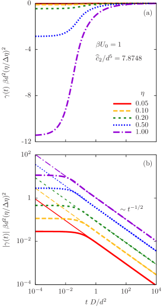
Figure 2: Non-equilibrium interfacial tension $\gamma(t)$ during the relaxation of polymer solutions described by a Gaussian core model Eq. (39) with polymer number densities $\bar{\varrho}$ corresponding to packing fractions $\eta=\pi\bar{\varrho}d^{3}/6\in\{0.05,0.1,0.2,0.5,1\}$. Thick lines represent the full expression Eq. (35), whereas thin lines in panel (b) correspond to the long-time asymptotics Eq. (38). Panel (a) shows that, for this system, the interfacial tension is negative, $\gamma(t)<0$, for all times $t\geq 0$. From panel (b) one can infer that the asymptotic expression Eq. (38) applies for times $t\gtrsim d^{2}/D$.

Figure 2 displays the temporal evolution of the interfacial tension $\gamma(t)$ for the case of interaction strength $\beta U_{0}=1$ and packing fractions $\eta:=\pi\bar{\varrho}d^{3}/6\in\{0.05,0.1,0.2,0.5,1\}$. The thick lines correspond to the full expression Eq. (35) based on the direct correlation function Eq. (40), whereas the thin lines in Fig. 2(b) are the long-time asymptotics Eq. (38). Note that, according to Eq. (35), the interfacial tension scales $\sim(\Delta\eta/\eta)^{2}$ with the initial relative density difference $\Delta\varrho/\varrho=\Delta\eta/\eta$.

The interfacial tension $\gamma(t)$ for this system turns out to be negative for all times $t\geq 0$ (see Fig. 2(a)) because $\widehat{\bar{c}}(q_{z})$ in Eq. (40) is a monotonically increasing function of $q_{z}$, i.e., $\widehat{\bar{c}}\,^{\prime}(q_{z})>0$, so that, according to Eq. (35), $\gamma(t)<0$. This is, in particular, in accordance with Eq. (38) and $\widehat{\bar{c}}_{2}>0$ from Eq. (42). Figure 2(b) indicates that the asymptotic behavior $\gamma(t)\sim t^{-1/2}$ in Eq. (38) can be expected to apply at times beyond the Brownian time scale $t\gtrsim d^{2}/D$; this statement applies to a wide range of the parameters $\beta U_{0}$ and $\eta$, the results of which are not shown here.

According to Refs. Kim1990 ; Francis2006 , the interaction potential Eq. (39) with interaction strength $\beta U_{0}=1.58$ and $d=R_{g}\sqrt{2/3}=60\,\text{nm}$ is valid to describe the interaction of pairs of poly($\alpha$-methyl styrene) chains with molecular mass $M_{w}=2.96\times 10^{6}\,\text{g/mol}$ in toluene at $25\,^{\circ}\text{C}$ in the dilute regime $\eta\lesssim 0.22$. At the Brownian time $t=d^{2}/D=46\,\text{ms}$, where $D=0.079\,\mu\text{m}^{2}/\text{s}$ is the experimental diffusion constant, one finds $\beta\gamma(t)d^{2}=-0.13(\Delta\eta/\eta)^{2}$ for $\eta=0.22$, i.e., for an initial perturbation of $|\Delta\eta|=0.1\eta$ the free energy $k_{\text{B}}T$ is gained by interface fluctuations which increase the interfacial area by $2.77\,\mu\text{m}^{2}$.

III.2 Charge-stabilized colloids

As a second example consider a colloidal suspension of charge-stabilized colloids of diameter $d$ in a solvent with inverse Debye length $\kappa$. Here the interaction of two colloidal particles is modeled by the potential

$$\beta U(r)=\begin{cases}\infty&,r\leq d\\ \displaystyle\beta U_{d}\frac{\exp(-\kappa(r-d))}{r/d}&,r>d,\end{cases}$$ (43)

where the strength $\beta U_{d}>0$ of the double layer repulsion increases with the charge of the colloids. The direct correlation function of the colloidal suspension within RPA of the double layer repulsion in excess to the hard-sphere reference system is given by

$$\bar{c}(r)=\begin{cases}c_{\text{HS}}(r)&,r\leq d\\ \displaystyle-\beta U_{d}\frac{\exp(-\kappa(r-d))}{r/d}&,r>d,\end{cases}$$ (44)

where the Percus-Yevick direct correlation function of hard spheres with diameter $d$ and packing fraction $\eta$ is Hansen1986

$$c_{\text{HS}}(r)=\begin{cases}\displaystyle c_{\text{HS}}^{(0)}(\eta)+c_{\text{HS}}^{(1)}(\eta)\frac{r}{d}+c_{\text{HS}}^{(3)}(\eta)\left(\frac{r}{d}\right)^{3}&,r\leq d\\ 0&,r>d\end{cases}$$ (45)

with

$$c_{\text{HS}}^{(0)}(\eta) =-\frac{(1+2\eta)^{2}}{(1-\eta)^{4}},$$

$$c_{\text{HS}}^{(1)}(\eta) =\frac{6\eta(1+\eta/2)^{2}}{(1-\eta)^{4}},$$

$$c_{\text{HS}}^{(3)}(\eta) =-\frac{\eta(1+2\eta)^{2}}{2(1-\eta)^{4}}.$$ (46)

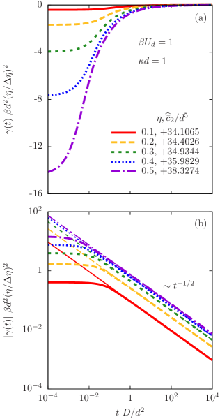
Figure 3: Non-equilibrium interfacial tension $\gamma(t)$ during the relaxation of suspensions of charge-stabilized colloids interacting via the potential Eq. (43) with strength $\beta U_{d}=1$ of the double layer repulsion, inverse Debye length $\kappa d=1$, and packing fractions $\eta\in\{0.1,0.2,0.3,0.4,0.5\}$. Thick lines represent the full expression Eq. (35), whereas thin lines in panel (b) correspond to the long-time asymptotics Eq. (38). Panel (a) shows that, for this system, the interfacial tension is negative, $\gamma(t)<0$, for all times $t\geq 0$. From panel (b) one can infer that the asymptotic expression Eq. (38) applies for times $t\gtrsim d^{2}/D$.

Figure 3 displays the temporal evolution of the interfacial tension $\gamma(t)$ for the case of interaction strength $\beta U_{d}=1$, inverse Debye length $\kappa d=1$, and packing fractions $\eta\in\{0.1,0.2,0.3,0.4,0.5\}$. The thick lines correspond to the full expression Eq. (35) based on the direct correlation function Eqs. (44)–(46), whereas the thin lines in Fig. 3(b) are the long-time asymptotics Eq. (38).

The interfacial tension $\gamma(t)$ for charge-stabilized colloids, as for polymer solutions in the previous Subsec. III.1, is negative, $\gamma(t)<0$, for all times $t\geq 0$ (see Fig. 3(a)), which is also in agreement with the positive values $\widehat{\bar{c}}_{2}>0$ entering in the long-time asymptotics Eq. (38). Figure 3(b) indicates that the asymptotic behavior $\gamma(t)\sim t^{-1/2}$ in Eq. (38) sets in, as for polymer solutions in the previous Subsec. III.1, at times beyond the Brownian time scale $t\gtrsim d^{2}/D$.

It has to be noted that the interaction strength $\beta U_{d}$ of some real charge-stabilized colloids can exceed unity by orders of magnitudes: In Ref. Crocker1994 , e.g., an aqueous dispersion ($\kappa^{-1}=161\,\text{nm}$) of polystyrene sulfate spheres of diameter $d=652\,\text{nm}$ and packing fraction $\phi\approx 0.04$ is reported with $\beta U_{d}=463$. For such a large value of $\beta U_{d}$ the RPA Eq. (44) is not justified so that one has to use more reliable schemes to evaluate $\bar{c}(r)$.

III.3 Colloid-polymer mixtures

As a final example consider a colloid-polymer mixture composed of colloidal hard spheres of diameter $d$ suspended in a solution of polymer coils of diameter $\ell$. Within the Asakura-Oosawa-Vrij theory Asakura1954 ; Asakura1958 ; Vrij1976 , the polymer coils with packing fraction $\eta_{\text{p}}$ give rise to an effective depletion interaction

$$\beta V(r)=-\eta_{\text{p}}\left(1+\frac{d}{\ell}\right)^{3}\left(1-\frac{3r}{2(d+\ell)}+\frac{r^{3}}{2(d+\ell)^{3}}\right)$$ (47)

between colloidal particles for distances in the range $r\in(d,d+\ell)$. The direct correlation function of the colloidal suspension within RPA of the depletion interaction in excess to the hard-sphere reference system is given by

$$\bar{c}(r)=\begin{cases}c_{\text{HS}}(r)&,r\leq d\\ -\beta V(r)&,r\in(d,d+\ell)\\ 0&,r\geq d+\ell.\end{cases}$$ (48)

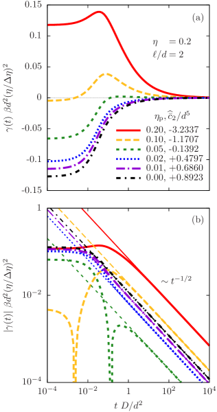
Figure 4: Non-equilibrium interfacial tension $\gamma(t)$ during the relaxation of colloid-polymer mixtures described within the Asakura-Oosawa-Vrij model Eq. (47) with colloidal packing fraction $\eta=0.2$, polymer-to-colloid size ratio $\ell/d=2$ and polymer packing fractions $\eta_{p}\in\{0,0.01,0.02,0.05,0.1,0.2\}$. Thick lines represent the full expression Eq. (35), whereas the thin lines in panel (b) correspond to the long-time asymptotics Eq. (38). Panel (a) demonstrates that the interfacial tension $\gamma(t)$ as a function of time $t$ can be positive ($\gamma(t)>0$, see case $\eta_{p}=0.2$) or negative ($\gamma(t)<0$, see cases $\eta_{p}\in\{0,0.01,0.02\}$) or it can change its sign (see cases $\eta_{p}\in\{0.05,0.1\}$). From panel (b) one can infer that the asymptotic expression Eq. (38) applies for times $t\gtrsim d^{2}/D$.

Figure 4 displays the temporal evolution of the interfacial tension $\gamma(t)$ for the colloidal packing fraction $\eta=0.2$, the size ratio $\ell/d=2$, and the polymer packing fractions $\eta_{\text{p}}\in\{0,0.01,0.02,0.05,0.1,0.2\}$. The thick lines correspond to the full expression Eq. (35) based on the direct correlation function Eq. (48), whereas the thin lines in Fig. 4(b) are the long-time asymptotics Eq. (38).

In accordance with Eq. (38), the asymptotic decay $\gamma(t)\to 0$ is from below for weak depletion attractions, $\eta_{\text{p}}\in\{0,0.01,0.02\}$, with positive values $\widehat{\bar{c}}_{2}>0$, whereas it is from above for strong depletion attractions, $\eta_{\text{p}}\in\{0.05,0.1,0.2\}$, with negative values $\widehat{\bar{c}}_{2}<0$. This demonstrates that it can be possible to alter the sign of the asymptotic decay by simply changing the polymer concentration. Moreover, the cases $\eta_{p}\in\{0.05,0.1\}$ in Fig. 4 show that the sign of the interfacial tension $\gamma(t)<0$ at early times $t\to 0$ has no influence on the sign $\gamma(t)>0$ at late times $t\to\infty$. Figure 4(b) indicates that also in these systems the asymptotic behavior $\gamma(t)\sim t^{-1/2}$ in Eq. (38) can be expected to apply at times beyond the Brownian time scale $t\gtrsim d^{2}/D$.

IV Conclusions

It has been shown in Sec. II that, under the mild conditions of an interaction potential $U(r)$ decaying for $r\to\infty$ faster than $\sim r^{s}$ with $s>5$ (see Subsec. II.1) and of an underlying model B dynamics (see Subsec. II.2), an initially perturbed colloidal fluid relaxes towards equilibrium accompanied by a time-dependent non-equilibrium interfacial tension $\gamma(t)$ which is not necessarily positive.

Here the non-equilibrium interfacial tension $\gamma(t)$ is defined via the work required to deform the system such that the interfacial area changes while the fluid volume is preserved (see Subsec. II.3). An experimental determination of the non-equilibrium interfacial tension $\gamma(t)$ requires, on the one hand, a sufficiently slow dynamics of the system such that the structure does not change appreciably during the measurement and, on the other hand, a sufficiently fast dynamics to preserve local equilibrium during deformation. Colloidal suspensions and polymer solutions with their wide separation of solvent and solute time scales (nanoseconds vs. milliseconds) are systems for which the negative non-equilibrium interfacial tension could be realized. There the fluid, whose non-equilibrium interfacial tension is to be measured, is formed by the colloidal particles, whereas the solvent acts as a medium whose Stokes flow due to agitation of the container walls leads to the deformation of the colloidal fluid.

The non-equilibrium interfacial tension $\gamma(t)$ is, under the above-mentioned conditions, determined by the equilibrium structure, the diffusion constant, and the initial density difference $\Delta\varrho$ from equilibrium (see Subsec. II.4). In particular, Eq. (35) leads to $\gamma(t)\sim\Delta\varrho^{2}$, which is reminiscent of the expression for the interfacial tension of equilibrium interfaces within the square-gradient approximation Rowlinson2002 . However, the square-gradient approximation is applicable only, if the square-gradient contribution, and hence the interfacial tension, is positive, because otherwise all uniform bulk states would be unstable with respect to density fluctuations. A positive square-gradient contribution corresponds to a negative coefficient $\widehat{\bar{c}}_{2}<0$ of the quadratic term $\sim q^{2}$ in Eq. (1), but this term is not required to be negative beyond square-gradient approaches, where the higher-order terms $\mathcal{R}(q)$ are not neglected. The interesting and rather general finding Eq. (38) shows that the long-time limit $\gamma(t\to\infty)$ is proportional to this coefficient $\widehat{\bar{c}}_{2}$ of the quadratic contribution $\sim q^{2}$ in Eq. (1). The reason is that the relaxation time $\tau(q)$ in Eq. (15) decreases with increasing wave number $q$ so that the contributions of large wave numbers $q$ decay quickly (see Eq. (35)).

Several examples of realistic systems have been proposed in Sec. III for which negative non-equilibrium interfacial tensions $\gamma(t)$ during relaxation can be expected to occur: Polymer solutions (Subsec. III.1, Fig. 2), charge-stabilized colloids (Subsec. III.2, Fig. 3), and colloid-polymer mixtures (Subsec. III.3, Fig. 4). The latter system even offers the possibility to switch between an asymptotically positive ($\gamma(t\to\infty)>0$) and an asymptotically negative ($\gamma(t\to\infty)<0$) non-equilibrium interfacial tension. As a rule of thumb, $\widehat{\bar{c}}_{2}<0$, and hence $\gamma(t\to\infty)>0$, corresponds to an interaction potential $U(r)$ with the attractive contribution being sufficiently strong as compared to the repulsive contribution, whereas $\widehat{\bar{c}}_{2}>0$, and hence $\gamma(t\to\infty)<0$, is the result of an interaction potential $U(r)$ with the repulsive contribution being sufficiently strong as compared to the attractive contribution.

Positive and negative values of the non-equilibrium interfacial tension $\gamma(t)$ lead to different morphologies of density perturbations: The relaxation towards a uniform equilibrium state takes place by minimizing the interfacial area for $\gamma(t)>0$ and by maximizing the interfacial area for $\gamma(t)<0$. Hence, localized density perturbations tend to spatially shrink with interfaces being smooth for $\gamma(t)>0$ while they tend to spread out with increasingly rough interfaces for $\gamma(t)<0$.

It is important to realize that the relaxation of a density perturbation is not driven by the non-equilibrium interfacial tension, which can be positive or negative (Fig. 4(a)), but by the non-uniformity of the local chemical potential (see Eq. (5)); the interfacial tension is merely related to the interfacial structure formed during the relaxation process. It is straightforward to show with Eqs. (5), (7), and (8) that the Helmholtz free energy $F[\varrho(t)]$ is a monotonically decreasing function of time $t$,

$$\frac{\mathrm{d}F[\varrho(t)]}{\mathrm{d}t}=-\frac{1}{\beta D}\int\mathrm{d}^{3}r\,\frac{\mathbf{j}(\mathbf{r},t)^{2}}{\varrho(\mathbf{r},t)}<0,$$ (49)

and it is this decrease which leads to the irreversibility of the relaxation towards equilibrium. In contrast, the non-equilibrium interfacial tension in Eq. (31) quantifies the linear response of the system to reversible deformations, and it has been shown in Sec. II.3 that this linear response is independent of the type of deformation. Beyond linear response one may find a dependence of the system’s response on the type of deformation, but such a behavior has to be described by a different quantity than the interfacial tension.

Based on these comments, one can reconcile the non-equilibrium interfaces during relaxation studied in the present work with equilibrium interfaces between two coexisting bulk phases: First, equilibrium interfaces, whose interfacial tensions do not vanish, exhibit a time-independent structure because the local chemical potential in equilibrium is uniform. Second, bulk coexistence is possible only for a sufficiently strong attractive contribution to the interaction potential $U(r)$ as compared to the repulsive contribution, which typically leads to $\widehat{\bar{c}}_{2}<0$, i.e., $\gamma(t\to\infty)>0$. Conversely, a negative equilibrium interfacial tension requires an interaction potential $U(r)$ with the repulsive contribution dominating the attractive one, but under these condition no bulk coexistence, and thus no equilibrium interface, occurs.

In conclusion, a rather general expression for the interfacial tension of a relaxing planar non-equilibrium interface is derived and applied to realistic systems of colloidal suspensions and polymer solutions. It is shown that the non-equilibrium interfacial tension is not necessarily positive, that negative non-equilibrium interfacial tensions are consistent with strictly positive equilibrium interfacial tensions, and that the sign of the interfacial tension can influence the morphology of density perturbations during relaxation. The present study highlights that the useful concept of a non-equilibrium interfacial tension shares some but not all properties with the equilibrium interfacial tension. Until now concepts of non-equilibrium interfacial tensions have been introduced only for systems close to equilibrium, whose known relaxation dynamics towards equilibrium allows for generalizations of the equilibrium interfacial tension. It is a future task of enormous relevance to understand the properties of non-equilibrium interfaces also far away from equilibrium. Whether the interfacial tension is a useful concept also far away from equilibrium or whether its applicability is restricted to the vicinity of equilibrium is an interesting open question.

References

- (1) S.A. Safran, Statistical Thermodynamics of Surfaces, Interfaces, and Membranes (Westview, Boulder, 2003).
- (2) P.-G. de Gennes, F. Brochard-Wyart, and D. Queré, Capillarity and Wetting Phenomena (Springer, New York, 2004).
- (3) J.S. Rowlinson and B. Widom, Molecular theory of capillarity (Dover, Mineola, 2002).
- (4) P. Joos, Dynamic Surface Phenomena (VSP, Utrecht, 1999).
- (5) J. Drelich, Ch. Fang, and C.L. White, Interfacial Tension Measurement in Fluid-Fluid Systems, in Encyclopedia of Surface and Colloid Science, Vol. 4, edited by P. Somasundaran (Taylor & Francis, New York, 2006), p. 2966.
- (6) S. Peach and C. Franck, J. Chem. Phys. 104, 686 (1996).
- (7) C. Maze and G. Burnet, Surf. Sci. 27, 411 (1971).
- (8) Z. Adamczyk, J. Colloid Interface Sci. 120, 477 (1987).
- (9) R. Millner, P. Joos, and V.B. Fainerman, Adv. Colloid Interface Sci. 49, 249 (1994).
- (10) J. Eastoe and J.S. Dalton, Adv. Colloid Interface Sci. 85, 103 (2000).
- (11) P. Cicuta, A. Vailati, and M. Giglio, Phys. Rev. E 62, 4920 (2000).
- (12) M. Bier and D. Arnold, Phys. Rev. E 88, 062307 (2013).
- (13) V.I. Levitas, Phys. Rev. B 89, 094107 (2014).
- (14) R. Evans, Adv. Phys. 28, 413 (1979).
- (15) W. Dieterich, H.L. Frisch, and A. Majhofer, Z. Phys. B 78, 317 (1990).
- (16) K. Kawasaki, Physica A 208, 35 (1994).
- (17) D. Dean, J. Phys. A 29, L613 (1996).
- (18) U. Marini Bettolo Marconi and P. Tarazona, J. Chem. Phys. 110, 8032 (1999).
- (19) U. Marini Bettolo Marconi and P. Tarazona, J. Phys.: Condens. Matter 12, A413 (2000).
- (20) P.C. Hohenberg and D. Halperin, Rev. Mod. Phys. 49, 435 (1977).
- (21) F.H. Stillinger, J. Chem. Phys. 65, 3968 (1976).
- (22) P.J. Flory and W.R. Krigbaum, J. Chem. Phys. 18, 1086 (1950).
- (23) S.H. Kim, D.J. Ramsay, and G.D. Patterson, J. Polym. Sci. 28, 2023 (1990).
- (24) R.S. Francis, G.D. Patterson, and S.H. Kim, J. Polym. Sci. 44, 703 (2006).
- (25) J.-P. Hansen and I.R. McDonald, Theory of simple liquids (Academic Press, San Diego, 1986).
- (26) J.C. Crocker and D.G. Grier, Phys. Rev. Lett. 73, 352 (1994).
- (27) S. Asakura and F. Oosawa, J. Chem. Phys. 22, 1255 (1954).
- (28) S. Asakura and F. Oosawa, J. Polymer Sci. 33, 183 (1958).
- (29) A. Vrij, Pure Appl. Chem. 48, 471 (1976).