Uniform Asymptotics for Nonparametric Quantile Regression with an Application to Testing Monotonicity

Abstract.

In this paper, we establish a uniform error rate of a Bahadur representation for local polynomial estimators of quantile regression functions. The error rate is uniform over a range of quantiles, a range of evaluation points in the regressors, and over a wide class of probabilities for observed random variables. Most of the existing results on Bahadur representations for local polynomial quantile regression estimators apply to the fixed data generating process. In the context of testing monotonicity where the null hypothesis is of a complex composite hypothesis, it is particularly relevant to establish Bahadur expansions that hold uniformly over a large class of data generating processes. In addition, we establish the same error rate for bootstrap local polynomial estimators which can be useful for various bootstrap inference. As an illustration, we apply to testing monotonicity of quantile regression and present Monte Carlo experiments based on this example.

Key words. Bootstrap, conditional moment inequalities, kernel estimation, local polynomial estimation, $L_{p}$ norm, nonparametric testing, Poissonization, quantile regression, testing monotonicity, uniform asymptotics

1. Introduction

In this paper, we establish a Bahadur representation of a local polynomial estimator of a nonparametric quantile regression function that is uniform over a range of quantiles, a range of evaluation points in the regressors, and a wide class of probabilities underlying the distributions of observed random variables. We also establish a Bahadur representation for a bootstrap estimator of a nonparametric quantile regression function.

There are several existing results of Bahadur representation of the local polynomial quantile regression estimator in the literature. Chaudhuri:91a is the classical result on a local polynomial quantile regression estimator with a uniform kernel. His result is pointwise in that the representation holds at one quantile, for a fixed point, and for a given data generating process. For recent contributions that are closely related to this paper, see Kong/Linton/Xia:10, Guerre/Sabbah:12, Kong/Linton/Xia:13, and Qu:Yoon:15, among others. Kong/Linton/Xia:10 obtain a Bahadur representation for a local polynomial M-estimator, including the quantile regression estimator as a special case, for strongly mixing stationary processes. Their result holds uniformly for a range of evaluation points in the regressors but at a fixed quantile for a given data generating process. Guerre/Sabbah:12 obtain Bahadur representations that hold uniformly over a range of quantiles, a range of evaluation points in the regressors, and a range of bandwidths for independent and identically distributed (i.i.d.) data. However, their result is for a fixed data generating process. Kong/Linton/Xia:13 extend to the case when the dependent variable is randomly censored for i.i.d. data and obtain the representation that is uniform over the evaluation points. Qu:Yoon:15 consider estimating the conditional quantile process nonparametrically for the i.i.d. data using local linear regression, with a focus on quantile monotonicity. They develop a Bahadur representation that is uniform in the quantiles but at a fixed evaluation point for a given data generating process. It seems that our work is the first that obtains a Bahadur representation that holds uniformly over the triple: the quantile, the evaluation point, and the underlying distribution. However, our result is for a fixed bandwidth, unlike Guerre/Sabbah:12.

The most distinctive feature of our result is that the Bahadur representation is uniform over a wide class of probabilities. Uniformity of asymptotic approximation in probabilities has long drawn interest in statistical decision theory and empirical process theory. Uniformity in asymptotic approximation is generally crucial for procuring finite sample stability of size or coverage probability in inference. See Andrews/Cheng/Guggenberger:11 for its emphasis and general tools for uniform asymptotic results. In the recent literature of econometrics, identifying the class of probabilities for which the uniformity holds, and their plausibility in practice, have received growing attention, along with increasing interests in models based on inequality restrictions. See, for example, Andrews/Soares:10 and Andrews/Shi:13a among many others.

To see the issue of uniformity, consider a simple testing problem:

(1.1) $$H_{0}:\forall x\in\mathcal{X},\ \frac{\partial\mathrm{Med}\left[Y|X=x\right]}{\partial x}\geq 0\;vs.\;H_{1}:\exists x\in\mathcal{X},\ \frac{\partial\mathrm{Med}\left[Y|X=x\right]}{\partial x}<0,$$

where $\mathrm{Med}\left[Y|X=x\right]$ is the conditional median of $Y$ given $X=x$ and $\mathcal{X}$ is a region of interest. Then one may develop a nonparametric test statistic using the local polynomial quantile regression estimator (e.g. the $L_{p}$ statistic as in Section 3). The behavior of this nonparametric test statistic depends crucially on the contact set $B:=\{x\in\mathcal{X}:\ {\partial\mathrm{Med}\left[Y|X=x\right]}/{\partial x}=0\}$. To emphasize the issue of uniformity, consider a sequence of data generating processes indexed by $n$. For example, we take the sequence of the true conditional median functions to be $\mathrm{Med}_{n}\left[Y|X=x\right]=x^{3}/n$ on $\mathcal{X}=[-1,1]$. Then for each $n$, the corresponding contact set is a singleton set, that is $B_{n}=\{0\}$; however, $\mathrm{Med}_{n}\left[Y|X=x\right]=x^{3}/n$ converges to $0$ uniformly in $x\in\mathcal{X}$ as $n\rightarrow\infty$. In other words, as $n$ gets large, the true function looks flat on $\mathcal{X}$, but the population contact set is always the singleton set at zero for each $n$. This suggests that the pointwise asymptotic theory may not be adequate for finite sample approximation. Therefore, it is important to develop uniform asymptotics for the local polynomial quantile regression estimator by establishing the Bahadur representation that is uniform over a large class of probabilities.

We illustrate the usefulness of our Bahadur representation by applying it to testing monotonicity of quantile regression that includes (1.1) as a special case. Our proposed test uses the framework of [LSW hereafter]LSW. They provide a general method of testing inequality restrictions for nonparametric functions, and make use of this paper’s result in establishing sufficient conditions for one of their results.

The remainder of the paper is as follows. Section 2 presents the main results of the paper, Section 3 gives an application of our main results in the context of testing monotonicity, Section 4 concludes, and Section 5 gives all the proofs.

2. Uniform Asymptotics

This section provides uniform Bahadur representations for local polynomial quantile regression estimators and considers their bootstrap version as well.

2.1. Uniform Bahadur Representation for Local Polynomial Quantile Regression Estimators

In this subsection, we present a Bahadur representation of a local polynomial quantile regression estimator that can be useful for a variety of purposes.

Let $(B^{\top},X^{\top},L)^{\top}$, with $B\equiv(B_{1},...,B_{\bar{L}})^{\top}\in\mathbf{R}^{\bar{L}}$, and $X\in\mathbf{R}^{d}$, be a random vector such that the joint distribution of $(B^{\top},X^{\top})^{\top}$ is absolutely continuous with respect to Lebesgue measure and $L$ is a discrete random variable taking values from $\mathbb{N}_{L}\equiv\{1,2,...,\bar{L}\}$. For each $x\in\mathbf{R}^{d}$ and $k\in\mathbb{N}_{L}$, we assume that the conditional distribution of $B_{l}$ given $(X,L)=(x,k)$ is the same across $l=1,...,k$. It is unconventional to consider a vector $B$, but it is useful to do so here to cover the case where we observe multiple outcomes from the same conditional distribution.

Let $q_{k}(\tau|x)$ denote the $\tau$-th quantile of $B_{l}$ conditional on $X=x$ and $L=k,$ where $\tau\in(0,1)$. That is, $P\{B_{l}\leq q_{k}(\tau|x)|X=x,L=k\}=\tau$ for all $x$ in the support of $X$ and all $k\in\{1,...,\bar{L}\}$. We write

$$B_{l}=q_{k}(\tau|X)+\varepsilon_{\tau,lk},\text{ }\tau\in(0,1),\text{ for all }k\in\{1,...,\bar{L}\},$$

where $\varepsilon_{\tau,lk}$ is a continuous random variable such that the $\tau$-th conditional quantile of $\varepsilon_{\tau,lk}$ given $X$ and $L=k$ is equal to zero.

Suppose that we are given a random sample $\{(B_{i}^{\top},X_{i}^{\top},L_{i})^{\top}\}_{i=1}^{n}$ of $(B^{\top},X^{\top},L)^{\top}$. Assume that $q_{k}(\tau|x)$ is $(r+1)$-times continuously differentiable with respect to $x$, where $r\geq 1$. We use a local polynomial estimator $\widehat{q}_{k}(\tau|x)$, similar to Chaudhuri:91a. For $u\equiv(u_{1},\ldots,u_{d})$, a $d$-dimensional vector of nonnegative integers, let $[u]=u_{1}+\cdots+u_{d}$. Let $A_{r}$ be the set of all $d$-dimensional vectors $u$ such that $[u]\leq r$, and let $|A_{r}|$ denote the number of elements in $A_{r}$. For $z=(z_{1},...,z_{d})^{\top}\in\mathbf{R}^{d}$ with $u=(u_{1},...,u_{d})^{\top}\in A_{r}$, let $z^{u}=\prod_{m=1}^{d}z_{m}^{u_{m}}$. Now define $c(z)=(z^{u})_{u\in A_{r}},$ for $z\in\mathbf{R}^{d}$. Note that $c(z)$ is a vector of dimension $|A_{r}|$. For $u=(u_{1},...,u_{d})^{\top}\in A_{r}$, and $r+1$ times differentiable map $f$ on $\mathbf{R}^{d}$, we define the following derivative:

$$(D^{u}f)(x)\equiv\frac{\partial^{[u]}}{\partial x_{1}^{u_{1}}\cdot\cdot\cdot\partial x_{d}^{u_{d}}}f(x),$$

where $[u]=u_{1}+\cdot\cdot\cdot+u_{d}$. Then we define $\gamma_{\tau,k}(x)\equiv\left(\gamma_{\tau,k,u}(x)\right)_{u\in A_{r}}$, where

$$\gamma_{\tau,k,u}(x)\equiv\frac{1}{u_{1}!\cdot\cdot\cdot u_{d}!}D^{u}q_{k}(\tau|x).$$

We construct an estimator $\hat{\gamma}_{\tau,k}(x)$ as follows. First, we define for each $\gamma\in\mathbf{R}^{|A_{r}|},$

$$S_{n,x,\tau,k}(\gamma)\equiv\sum_{i=1}^{n}1\{L_{i}=k\}\sum_{\ell=1}^{L_{i}}l_{\tau}\left[B_{\ell i}-\gamma^{\top}c\left(\frac{X_{i}-x}{h}\right)\right]K\left(\frac{x-X_{i}}{h}\right).$$

Then we construct

(2.1) $$\hat{\gamma}_{\tau,k}(x)\equiv\text{argmin}_{\gamma\in\mathbf{R}^{|A_{r}|}}S_{n,x,\tau,k}(\gamma),$$

where $l_{\tau}(u)\equiv u[\tau-1\{u\leq 0\}]$ for any $u\in\mathbf{R}$, $K_{h}(t)=K(t/h)/h^{d}$, $K$ is a $d$-variate kernel function, and $h$ is a bandwidth that goes to zero as $n\rightarrow\infty$.

In order to reduce the redundancy of the statements, let us introduce the following definitions.

Definition 1.

Let $\mathcal{G}$ be a set of functions $g_{v}:\mathbf{R}^{m}\rightarrow\mathbf{R}^{s}\$indexed by a set $\mathcal{V}$, and let $S\subset\mathbf{R}^{m}$ be a given set and for $\varepsilon>0$, let $S_{v}(\varepsilon)$ be an $\varepsilon$-enlargement of $S_{v}=\{x\in S:(x,v)\in S\times V\}$, i.e., $S_{v}(\varepsilon)=\{x+a:x\in S$ and $a\in[-\varepsilon,\varepsilon]^{m}\}.$ Then we define the following conditions for $\mathcal{G}$:
(a) B($S,\varepsilon$): $g_{v}$ is bounded on $S_{v}(\varepsilon)\$uniformly over $v\in\mathcal{V}.$
(b) BZ$(S,\varepsilon$): $g_{v}$ is bounded away from zero on $S_{v}(\varepsilon)\$uniformly over $v\in\mathcal{V}.$
(c) BD($S,\varepsilon,r$): $\mathcal{G}$ satisfies B$(S,\varepsilon)$ and $g_{v}$ is $r$ times continuously differentiable on $S_{v}(\varepsilon)$ with derivatives bounded on $S_{v}(\varepsilon)$ uniformly over $v\in\mathcal{V}.$
(d) BZD($S,\varepsilon,r$): $\mathcal{G}$ satisfies BZ$(S,\varepsilon)$ and $g_{v}$ is $r$ times continuously differentiable on $S_{v}(\varepsilon)$ with derivatives bounded on $S_{v}(\varepsilon)$ uniformly over $v\in\mathcal{V}.$
(e) LC: $g_{v}$ is Lipschitz continuous with Lipschitz coefficient bounded uniformly over $v\in V$.

Let $\mathcal{P}$ denote the collection of the potential joint distributions of $(B^{\top},X^{\top},L)^{\top}$ and define $\mathcal{V}=\mathcal{T}\times\mathcal{P}$, and for each $k\in\mathbb{N}_{L},$

(2.2) $$\mathcal{G}_{q}(k) = \left\{q_{k}(\tau|\cdot):(\tau,P)\in\mathcal{V}\right\},$$

$$\mathcal{G}_{f}(k) = \left\{f_{\tau,k}(\cdot|\cdot):(\tau,P)\in\mathcal{V}\right\},$$

$$\mathcal{G}_{L}(k) = \left\{P\left\{L_{i}=k|X_{i}=\cdot\right\}:P\in\mathcal{P}\right\},\text{ and}$$

$$\mathcal{G}_{f} = \left\{f(\cdot):P\in\mathcal{P}\right\},$$

where $f_{\tau,k}(0|x)$ being the conditional density of $B_{li}-q_{k}(\tau|X_{i})$ given $X_{i}=x$ and $L_{i}=k.$ Also, define

(2.3) $$\mathcal{G}_{f,2}(k)=\left\{f_{\cdot,k}(\cdot|\cdot):P\in\mathcal{P}\right\}\text{ and\ }\mathcal{G}_{\gamma}(k)=\left\{\gamma_{\cdot,k}(\cdot):P\in\mathcal{P}\right\}.$$

In other words, $\mathcal{G}_{f,2}(k)$ is the class of conditional densities $f_{\tau,k}(\cdot|x)$ indexed by $\tau$, $x$, and probabilities $P$, and $\mathcal{G}_{\gamma}(k)$ is the class of functions $\gamma_{\tau,k}(\cdot)$ indexed by $\tau$ and probabilities $P$. We make the following assumptions.

Assumption QR 1.

(i) $\mathcal{G}_{f}$ satisfies BD($\mathcal{S},\varepsilon,1)$.
(ii) For each $k\in\mathbb{N}_{L}$, $\mathcal{G}_{f}(k)$ and $\mathcal{G}_{L}(k)\$satisfy both BD($\mathcal{S},\varepsilon,1)$ and BZD($\mathcal{S},\varepsilon,1).$
(iii) For each $k\in\mathbb{N}_{L}$, $\mathcal{G}_{q}(k)\$satisfies BD($\mathcal{S},\varepsilon,r+1)$ for some $r\geq 1.$
(iv) For each $k\in\mathbb{N}_{L}$, $\mathcal{G}_{f,2}(k)$ and $\mathcal{G}_{\gamma}(k)\$satisfy LC.

Assumptions QR1(i) and (iii) are standard assumptions used in the local polynomial approach where one approximates $q_{k}(\cdot|x)$ by a linear combination of its derivatives through Taylor expansion, except only that the approximation here is required to behave well uniformly over $P\in\mathcal{P}$. Assumption QR1(ii) is made to prevent the degeneracy of the asymptotic linear representation of $\hat{\gamma}_{\tau,k}(x)-\gamma_{\tau,k}(x)$ that is uniform over $x\in\mathcal{S}_{\tau}(\varepsilon),\ \tau\in\mathcal{T}$ and over $P\in\mathcal{P}$. Assumption QR1(iv) requires that the conditional density function of $B_{li}-q_{k}(\tau|X_{i})$ given $X_{i}=x$ and $L_{i}=k$ and $\gamma_{\tau,k}(\cdot)$ behave smoothly as we perturb $\tau$ locally. This requirement is used to control the size of the function spaces indexed by $\tau$, so that when the stochastic convergence of random sequences holds, it is ensured to hold uniformly in $\tau$.

Let $||\cdot||$ denote the Euclidean norm throughout the paper. Assumption QR2 lists conditions for the kernel function and the bandwidth.

Assumption QR 2.

(i) $K$ is compact-supported, bounded, and Lipschitz continuous on the interior of its support, $\int K(u)du=1$, and $\int K\left(u\right)||u||^{2}du>0.$
(ii) As $n\rightarrow\infty,\ n^{-1/2}h^{-d/2}\log n+\sqrt{nh^{d}}h^{r+1}/\sqrt{\log n}\rightarrow 0,$ with $r$ in Assumption QR1(iii).

Assumption QR2 gives conditions for the kernel and the bandwidth. The condition for the bandwidth is satisfied if we take $h=Cn^{-s}$ for some constant $C$ with $s>0$ satisfying that $1/(d+2(r+1))<s<1/d$.

For any sequence of real numbers $b_{n}>0$, and any sequence of random vectors $Z_{n}$, we say that $Z_{n}/b_{n}\rightarrow_{P}0,$ $\mathcal{P}$-uniformly, or $Z_{n}=o_{P}(b_{n}),$ $\mathcal{P}$-uniformly, if for any $a>0$,

$$\underset{n\rightarrow\infty}{\limsup}\sup_{P\in\mathcal{P}}P\left\{||Z_{n}||>ab_{n}\right\}=0\text{.}$$

Similarly, we say that $Z_{n}=O_{P}(b_{n})$, $\mathcal{P}$-uniformly, if for any $a>0$, there exists $M>0$ such that

$$\underset{n\rightarrow\infty}{\limsup}\sup_{P\in\mathcal{P}}P\left\{||Z_{n}||>Mb_{n}\right\}<a\text{.}$$

Below, we establish a uniform Bahardur representation of $\sqrt{nh^{d}}H(\hat{\gamma}_{\tau,k}(x)-\gamma_{\tau,k}(x))$, where $H=\$diag$((h^{|u|})_{u\in A_{r}})$ is the $|A_{r}|\times|A_{r}|$ diagonal matrix. First we introduce some notation. We define

$$\Delta_{x,\tau,lk,i} \equiv B_{li}-\gamma_{\tau,k}^{\top}(x)c(X_{i}-x),$$

$$c_{h,x,i} \equiv c\left((X_{i}-x)/h\right),\text{ and }K_{h,x,i}\equiv K\left((X_{i}-x)/h\right).$$

Let

$$M_{n,\tau,k}(x)\equiv k\int P\{L_{i}=k|X_{i}=x+th\}f_{\tau,k}(0|x+th)f(x+th)K(t)c(t)c^{\top}(t)dt.$$

Theorem 1.

Suppose that Assumptions QR1-QR2 hold. Then, for each $k\in\mathbb{N}_{L},$

$$\sup_{\tau\in\mathcal{T},x\in\mathcal{S}_{\tau}(\varepsilon)}\left\|\sqrt{nh^{d}}H(\hat{\gamma}_{\tau,k}(x)-\gamma_{\tau,k}(x))-M_{n,\tau,k}^{-1}(x)\left(\psi_{n,x,\tau,k}-\mathbf{E}\psi_{n,x,\tau,k}\right)\right\|$$

$$= O_{P}\left(\frac{\log^{1/2}n}{n^{1/4}h^{d/4}}\right),\ \mathcal{P}\text{{-uniformly},}$$

where, with $\tilde{l}_{\tau}\left(x\right)\equiv\tau-1\{x\leq 0\}$,

$$\psi_{n,x,\tau,k}\equiv-\frac{1}{\sqrt{nh^{d}}}\sum_{i=1}^{n}1\left\{L_{i}=k\right\}\sum_{l=1}^{L_{i}}\tilde{l}_{\tau}\left(\Delta_{x,\tau,lk,i}\right)c_{h,x,i}K_{h,x,i}\text{.}$$

The proof in this paper uses the convexity arguments of Pollard:91 (see Kato:09 for a related recent result) and, similarly as in Guerre/Sabbah:12, employs the maximal inequality of [Theorem 6.8]Massart:07. The theoretical innovation of Theorem 1 is that we have obtained an approximation that is uniform in $(x,\tau)$ as well as in $P$. See Remark 1 below for a detailed comparison.

Remark 1.

The main difference between this paper and Guerre/Sabbah:12 is that their result pays attention to uniformity in $h$ over some range, while our result pays attention to uniformity in $P$. Also it is interesting to note that the error rate here is a slight improvement over theirs. When $d=1$, the rate here is $O_{P}[\sqrt{\log n}/(n^{1/4}h^{1/4})]$ while the rate in Theorem 2 of Guerre/Sabbah:12 is $O_{P}[\log^{3/4}n/(n^{1/4}h^{1/4})]$. The difference is due to our use of an improved inequality which leads to a tighter bound in the maximal inequality in deriving the uniform error rate. For details, see the remark after the proof of Theorem 1 in the appendix.

The summands in the asymptotic linear representation form in Theorem 1 depend on the sample size and are not centered conditional on $X_{i}$. While this form can be useful in some contexts, the form is less illuminating. We provide an asymptotic linear representation that ensures this conditional centering given $X_{i}$.

Corollary 1.

Suppose that Assumptions QR1-QR2 hold. Then, for each $k\in\mathbb{N}_{L},$

$$\sup_{\tau\in\mathcal{T},x\in\mathcal{S}_{\tau}(\varepsilon)}\left\|\sqrt{nh^{d}}H(\hat{\gamma}_{\tau,k}(x)-\gamma_{\tau,k}(x))-M_{n,\tau,k}^{-1}(x)\tilde{\psi}_{n,x,\tau,k}\right\|$$

$$= O_{P}\left(\frac{\log^{1/2}n}{n^{1/4}h^{d/4}}\right),\ \mathcal{P}\text{{-uniformly},}$$

where

$$\tilde{\psi}_{n,x,\tau,k}\equiv-\frac{1}{\sqrt{nh^{d}}}\sum_{i=1}^{n}1\left\{L_{i}=k\right\}\sum_{l=1}^{L_{i}}\tilde{l}_{\tau}\left(\varepsilon_{\tau,lk,i}\right)c_{h,x,i}K_{h,x,i}\text{.}$$

Note that the quantity $M_{n,\tau,k}(x)$ in the representation can be replaced by

$$M_{\tau,k}(x)\equiv k\int P\{L_{i}=k|X_{i}=x\}f_{\tau,k}(0|x)f(x)K(t)c(t)c^{\top}(t)dt,$$

if we modify the conditions on kernels and the smoothness conditions for the nonparametric function $P\{L_{i}=k|X_{i}=x\}f_{\tau,k}(0|x)f(x)$. As this modification can be done in a standard manner, we do not pursue details.

2.2. Bootstrap Uniform Bahadur Representation for Local Polynomial Quantile Regression Estimator

Let us consider the bootstrap version of the Bahadur representation in Theorem 1. Suppose that $\{(Y_{i}^{\ast\top},X_{i}^{\ast\top})\}_{i=1}^{n}$ is a bootstrap sample drawn with replacement from the empirical distribution of $\{(Y_{i}^{\top},X_{i}^{\top})_{i=1}^{n}\}$. Throughout the paper, the bootstrap distribution $P^{\ast}$ is viewed as the distribution of $(Y_{i}^{\ast},X_{i}^{\ast})_{i=1}^{n},$ conditional on $(Y_{i},X_{i})_{i=1}^{n}$, and let $\mathbf{E}^{*}$ be expectation with respect to $P^{*}$.

We define the notion of uniformity in the convergence of distributions under $P^{\ast}$. For any sequence of real numbers $b_{n}>0$, and any sequence of random vectors $Z_{n}^{\ast}$, we say that $Z_{n}^{\ast}/b_{n}\rightarrow_{P^{\ast}}0,$ $\mathcal{P}$-uniformly, or $Z_{n}^{\ast}=o_{P^{\ast}}(b_{n}),$ $\mathcal{P}$-uniformly, if for any $a>0$,

$$\underset{n\rightarrow\infty}{\limsup}\sup_{P\in\mathcal{P}}P\left\{P^{\ast}\left\{||Z_{n}^{\ast}||>ab_{n}\right\}>a\right\}=0\text{.}$$

Similarly, we say that $Z_{n}^{\ast}=O_{P^{\ast}}(b_{n})$, $\mathcal{P}$-uniformly, if for any $a>0$, there exists $M>0$ such that

$$\underset{n\rightarrow\infty}{\limsup}\sup_{P\in\mathcal{P}}P\left\{P^{\ast}\left\{||Z_{n}^{\ast}||>Mb_{n}\right\}>a\right\}<a\text{.}$$

For $z=(x,\tau)\in\mathcal{Z}$, define $\Delta_{x,\tau,lk,i}^{\ast}\equiv Y_{l,i}^{\ast}-\gamma_{\tau,k}^{\top}(x)c(X_{i}^{\ast}-x)$, and let $c_{h,x,i}^{\ast}$ and $K_{h,x,i}^{\ast}$ be $c_{h,x,i}$ and $K_{h,x,i}$ except that $X_{i}$ is replaced by $X_{i}^{\ast}$. Then the following theorem gives the bootstrap version of Theorem 1.

Theorem 2.

Suppose that Assumptions QR1-QR2 hold. Then for each $k\in\mathbb{N}_{J},$

$$\sup_{(x,\tau)\in\mathcal{X}_{1}\times\mathcal{T}}\left\|\sqrt{nh^{d}}H(\hat{\gamma}_{\tau,k}^{\ast}(x)-\hat{\gamma}_{\tau,k}(x))-M_{n,\tau,k}^{-1}(x)\left(\psi_{n,x,\tau,k}^{*}-\mathbf{E}^{*}\psi_{n,x,\tau,k}^{*}\right)\right\|$$

$$= O_{P^{\ast}}\left(\frac{\log^{1/2}n}{n^{1/4}h^{d/4}}\right),\text{ }\mathcal{P}\text{{-uniformly,}}$$

where $\psi_{n,x,\tau,k}^{\ast}\equiv-\frac{1}{\sqrt{nh^{d}}}\sum_{i=1}^{n}1\{L_{i}=k\}\sum_{l=1}^{k}\tilde{l}_{\tau}\left(\Delta_{x,\tau,lk,i}^{\ast}\right)c_{h,x,i}^{\ast}K_{h,x,i}^{\ast}$.

Theorem 2 is obtained by using Le Cam’s Poissonization Lemma (see [Proposition 2.5]Gine:97) and following the proof of Theorem 1. The bootstrap version of Corollary 1 follows immediately from Theorem 2.

3. Testing Monotonicity of Quantile Regression

This section considers testing monotonicity of quantile regression. We first state the testing problem formally, give the form of test statistic, verify regularity conditions, and present results of simple Monte Carlo experiments.

3.1. Testing Problem

Let $q(\tau|x)$ denote the $\tau$-th quantile of $Y$ conditional on $X=x$, where $\tau\in(0,1)$ and $X$ is a scalar random variable. In this subsection, we consider testing monotonicity of quantile regression. Define $g_{\tau}(x)\equiv\partial q(\tau|x)/\partial x$. The null hypothesis and the alternative hypothesis are as follows:

(3.1) $$H_{0} :g_{\tau}(x)\leq 0\ \text{for all }(\tau,x)\in\mathcal{T\times X}\text{ against}$$

$$H_{1} :g_{\tau}(x)>0\ \text{for some }(\tau,x)\in\mathcal{T}\times\mathcal{X},$$

where $\mathcal{X}$ is contained in the support of $X$ and $\mathcal{T}\subset(0,1)$. The null hypothesis states that the quantile functions are increasing on $\mathcal{X}$ for all $\tau\in\mathcal{T}$, and the alternative hypothesis is the negation of the hypothesis. If $\mathcal{T}$ is a singleton, then testing (3.1) amounts to testing monotonicity of quantile regression at a fixed quantile.

Suppose that $q(\tau|x)$ is continuously differentiable on $\mathcal{X}$ for each $\tau\in\mathcal{T}$. Then one natural approach is to test the sign restriction of the derivative of $q(\tau|x)$. In other words, we develop a test of inequality restrictions using the local polynomial estimator of $\partial q(\tau|x)/\partial x$.

One may consider various other forms of monotonicity tests for quantile regression. For example, one might be interested in monotonicity of an interquartile regression function. More specifically, let $\tau_{1}<\tau_{2}$ be chosen from $(0,1)$ and write $\Delta g_{\tau_{1},\tau_{2}}(x)\equiv g_{\tau_{2}}(x)-g_{\tau_{1}}(x)$. Then the null hypothesis and the alternative hypothesis of monotonicity of the interquartile regression function are as follows:

(3.2) $$H_{0,\Delta} : \Delta g_{\tau_{1},\tau_{2}}(x)\leq 0\ \text{for all }x\in\mathcal{X}\text{ against}$$

$$H_{1,\Delta} : \Delta g_{\tau_{1},\tau_{2}}(x)>0\ \text{for some }x\in\mathcal{X}\text{.}$$

The null hypothesis states that the interquartile regression function $q(\tau_{2}|x)-q(\tau_{1}|x)$ is increasing on $\mathcal{X}$. This type of monotonicity can be used to investigate whether the income inequality (in terms of interquartile comparison) becomes severe as certain demographic variable $X$ such as age increases.

3.2. Test Statistic

Suppose that we are given a random sample $\{(Y_{i},X_{i})\}_{i=1}^{n}$ of $(Y,X)$. First, we estimate $g_{\tau}(x)$ by local polynomial estimation to obtain, say, $\hat{g}_{\tau}(x)\equiv\mathbf{e}_{2}^{\top}\mathbf{\hat{\gamma}}_{\tau}(x)$, where $\mathbf{e}_{2}$ is a column vector whose second entry is one and the rest zero, and

(3.3) $$\mathbf{\hat{\gamma}}_{\tau}(x)\equiv\text{argmin}_{\mathbf{\gamma\in R}^{r+1}}\sum_{i=1}^{n}l_{\tau}\left(Y_{i}-\mathbf{\gamma}^{\top}c(X_{i}-x)\right)K_{h}(X_{i}-x).$$

This paper applies the general approach of LSW, and proposes a new nonparametric test of mononoticity hypotheses involving quantile regression functions. First, testing the monotonicity of $q(\tau|\cdot)$ is tantamount to testing nonnegativity of $g_{\tau}$ on a domain of interest. Define $\Lambda_{p}(a)=\left(\max\left\{a,0\right\}\right)^{p}$ for any real numbers $a>0$ and $p\geq 1.$ We consider two test statistics corresponding to the two testing problems discussed in Section 3.1: for $1\leq p<\infty,$

(3.4) $$T_{n,2} \equiv \int_{\mathcal{X}\times\mathcal{T}}\Lambda_{p}(\hat{g}_{\tau}(x))w_{\tau}(x)d(x,\tau)\text{, and}$$

$$T_{n}^{\Delta} \equiv \int_{\mathcal{X}}\Lambda_{p}(\Delta\hat{g}_{\tau_{1},\tau_{2}}(x))w(x)dx,\text{ }\tau_{1},\tau_{2}\in(0,1),$$

where $\Delta\hat{g}_{\tau_{1},\tau_{2}}(x)\equiv\hat{g}_{\tau_{2}}(x_{1})-\hat{g}_{\tau_{1}}(x_{1})$, $w_{\tau}(\cdot)$ and $w(\cdot)$ are nonnegative weight functions. The test statistic $T_{n,2}$ is used to test $H_{0}$ against $H_{1}$ and the test statistic $T_{n,\Delta}$ to test $H_{0,\Delta}$ against $H_{1,\Delta}$.

Let $\{(Y_{i}^{\ast},X_{i}^{\ast})\}$ be a bootstrap sample obtained from resampling from $\{(Y_{i},X_{i})\}_{i=1}^{n}$ with replacement. Then we define

(3.5) $$\mathbf{\hat{\gamma}}_{\tau}^{\ast}(x)\equiv\text{argmin}_{\mathbf{\gamma\in R}^{r+1}}\sum_{i=1}^{n}l_{\tau}\left(Y_{i}^{\ast}-\mathbf{\gamma}^{\top}c(X_{i}^{\ast}-x)\right)K_{h}(X_{i}^{\ast}-x)$$

and take $\hat{g}_{\tau}^{\ast}(x)\equiv\mathbf{e}_{2}^{\top}\mathbf{\hat{\gamma}}_{\tau}^{\ast}(x)$, similarly as before. We construct the “recentered” bootstrap test statistics:

(3.6) $$T_{n,2}^{\ast} \equiv \int_{\mathcal{X}\times\mathcal{T}}\Lambda_{p}\left(\hat{g}_{\tau}^{\ast}(x)-\hat{g}_{\tau}(x)\right)w_{\tau}(x)d(x,\tau),\text{ and}$$

$$T_{n,\Delta}^{\ast} \equiv \int_{\mathcal{X}}\Lambda_{p}\left(\Delta\hat{g}_{\tau_{1},\tau_{2}}^{\ast}(x)-\Delta\hat{g}_{\tau_{1},\tau_{2}}(x)\right)w(x)dx,$$

where $\Delta\hat{g}_{\tau_{1},\tau_{2}}^{\ast}(x)\equiv\hat{g}_{\tau_{2}}^{\ast}(x)-\hat{g}_{\tau_{1}}^{\ast}(x)$. We can now take the bootstrap critical values $c_{2,\alpha}^{\ast}$ and $c_{\Delta,\alpha}^{\ast}$ to be the $(1-\alpha)$ quantiles from the bootstrap distributions of $T_{n,2}^{\ast}$ and $T_{n,\Delta}^{\ast}$. Then we define

$$c_{2,\alpha,\eta}^{\ast}=\max\{c_{2,\alpha}^{\ast},h^{1/2}\eta+\hat{a}_{2}^{\ast}\}\text{ and\ }c_{\Delta,\alpha,\eta}^{\ast}=\max\{c_{\Delta,\alpha}^{\ast},h^{1/2}\eta+\hat{a}_{\Delta}^{\ast}\},$$

where$\ \hat{a}_{2}^{\ast}\equiv\mathbf{E}^{\ast}T_{n,2}^{\ast}$ and $\hat{a}_{\Delta}^{\ast}\equiv\mathbf{E}^{\ast}T_{n,\Delta}^{\ast}$. The $(1-\alpha)$-level bootstrap tests for the two hypotheses are defined as

(3.7)

$$\text{Reject }H_{0}$$ .

3.3. Primitive Conditions

We present primitive conditions for the asymptotic validity of the proposed monotonicity tests. Let $\mathcal{P}$ denote the collection of the potential joint distributions of $(Y,X)^{\top}$ and define $\mathcal{V}=\mathcal{T}\times\mathcal{P}$ as before. We also define $\mathcal{\tilde{V}}=\mathcal{T}^{2}\times\mathcal{P}$ and define $\mathcal{G}_{f}$ as in (2.2). Similarly as in (2.2), we introduce the following definitions:

$$\mathcal{G}_{g} = \left\{g_{\tau}(\cdot):(\tau,P)\in\mathcal{V}\right\},$$

$$\mathcal{G}_{\Delta g} = \{\Delta g_{\tau_{1},\tau_{2}}(\cdot):(\tau_{1},\tau_{2},P)\in\mathcal{\tilde{V}\}},\text{ and}$$

$$\mathcal{G}_{Q,f} = \left\{f_{\tau}(\cdot|\cdot):(\tau,P)\in\mathcal{V}\right\},$$

where $f_{\tau}(0|x)$ being the conditional density of $Y_{i}-q(\tau|X_{i})$ given $X_{i}=x.$ Also, define

$$\mathcal{G}_{f,2}=\left\{f_{\cdot}(\cdot|\cdot):P\in\mathcal{P}\right\}\text{ and\ }\mathcal{G}_{\gamma}=\left\{\gamma_{\cdot}(\cdot):P\in\mathcal{P}\right\}.$$

We make the following assumptions.

Assumption MON 1.

(i) $\mathcal{G}_{f}$ satisfies BD($\mathcal{S},\varepsilon,1)$.
(ii) $\mathcal{G}_{Q,f}\$satisfies both BD($\mathcal{S},\varepsilon,1$) and BZD($\mathcal{S},\varepsilon,1).$
(iii) $\mathcal{G}_{g}\$satisfies BD($\mathcal{S},\varepsilon,r+1$) for some $r>3/2.$
(iv) $\mathcal{G}_{f,2}$ and $\mathcal{G}_{\gamma}$ satisfy LC.

Assumption MON 2.

(i) $K$ is nonnegative and satisfies Assumption QR2(i).
(ii) $n^{-1/2}h^{-\{(3+\nu)/2\}+1}+\sqrt{n}h^{r+2}/\sqrt{\log n}\rightarrow 0,$ as $n\rightarrow\infty,\$for some small $\nu>0$, with $r$ in Assumption MON1(iii).

Assumption MON1 introduces a set of regularity conditions for various function spaces. Conditions (i)-(iii) require smoothness conditions. In particular, Condition (iii) is used to control the bias of the nonparametric quantile regression derivative estimator. Condition (iv) is analogous to Assumption QR1(iv) and used to control the size of the function space properly. Assumption MON2 introduces conditions for the kernel and bandwidth. The condition in Assumption MON2(ii) requires a bandwidth condition that is stronger than that in Assumption QR2(ii).

Assumptions IQM1-IQM2 below are used for testing $H_{0,\Delta}$.

Assumption IQM 1.

(i) Assumptions MON1(i),(ii) and (iv) hold.
(ii) $\mathcal{G}_{\Delta g}\$satisfies BD($\mathcal{S},\varepsilon,r+1)$ for some $r>3/2.$

Assumption IQM 2.

The kernel function $K$ and the bandwidth $h$ satisfy Assumption MON2.

The following result establishes the uniform validity of the bootstrap test. Let $\mathcal{P}_{0}\subset\mathcal{P}$ denote the set of potential distributions of the observed random vector under the null hypothesis.

Theorem 3.

(i) Suppose that Assumptions MON1-MON2 hold. Then,

$$\limsup_{n\rightarrow\infty}\sup_{P\in\mathcal{P}_{0}}P\{T_{n,2}>c_{2,\alpha,\eta}^{\ast}\}\leq\alpha.$$

(ii) Suppose that Assumptions IQM1-IQM2 hold. Then,

$$\limsup_{n\rightarrow\infty}\sup_{P\in\mathcal{P}_{0}}P\left\{T_{n,\Delta}>c_{\Delta,\alpha,\eta}^{\ast}\right\}\leq\alpha.$$

Using the general framework of LSW, it is possible to establish the consistency and local power of the test. Furthermore, it is also feasible to obtain a more powerful (but still asymptotically uniformly valid) test by estimating a contact set at the expense of requiring an additional tuning parameter (see LSW for details).

3.4. Monte Carlo Experiments

In this subsection, we present results of some Monte Carlo experiments that illustrate the finite-sample performance of one of the proposed tests. Specifically, we consider the following null and alternative hypotheses:

$$H_{0}:\forall x\in\mathcal{X},\ g(x)\geq 0\;vs.\;H_{1}:\exists x\in\mathcal{X},\ g(x)<0,$$

where $g(x)\equiv\partial\mathrm{Median}\left[Y|X=x\right]/\partial x$. In the experiments, $X$ is generated independently from $\text{Unif}[0,1]$ and $U$ follows the distribution of $X^{4}\times\mathbf{N}(0,0.1)$.

To check the size of the test, we generated $Y=U$, which we call the null model. Note that the null model corresponds to the least favorable case. To see the power of the test, we considered the following alternative models: $Y=m_{j}(X)+U$ $(j=1,2,3,4,5)$, where

$$m_{1}(x) = x(1-x),$$

$$m_{2}(x) = -0.1x,$$

$$m_{3}(x) = -0.1\exp(-50(x-0.5)^{2}),$$

$$m_{4}(x) = x+0.6\exp(-10x^{2}),$$

$$m_{5}(x) = [10(x-0.5)^{3}-2\exp(-10(x-0.5)^{2})]1(x<0.5)$$

$$+[0.1(x-0.5)-2\exp(-10(x-0.5)^{2})]1(x\geq 0.5).$$

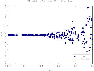
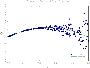
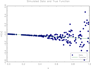
Figure 1. True Function and Simulated Data

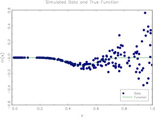
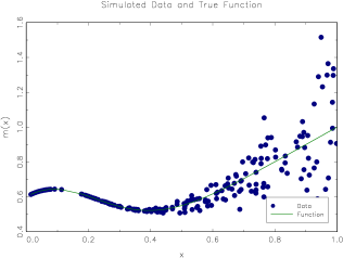
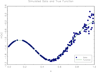
Figure 2. True Function and Simulated Data

In all experiments, $\mathcal{X}=[0.05,0.95]$. Figures 1 and 2 show the true functions and corresponding simulated data.

The experiments use sample size of $n=200$ and the nominal level of $\alpha=0.10,0.05,$ and $0.01.$ We performed $1,000$ Monte Carlo replications for the null model and $200$ replications for the alternative models. For each replication, we generated $200$ bootstrap resamples. We used the local linear quantile regression estimator with the uniform kernel on $[-1/2,1/2]\$for $K(\cdot)$. Furthermore, for the test statistic, we used $p=2$ (one-sided $L_{2}$ norm) and uniform weight function $w(x)=1$ and $h\in\{0.9,1,1.1\}$.

For the null model, the bootstrap approximation is quite good, especially with $h=1$. The test shows good power for alternative models 1-3 and 5. For the alternative model 4, the power is sensitive with respect to the choice of the bandwidth. Overall, the finite sample behavior of the proposed test is satisfactory.

4. Conclusions

In this paper, we have established a uniform error rate of a Bahadur representation for the local polynomial quantile regression estimator. The error rate is uniform over a range of quantiles, a range of evaluation points in the regressors, and over a wide class of probabilities for observed random variables. We have illustrated the use of our Bahadur representation in the context of testing monotonicity. In addition, we have established the same error rate for the bootstrap local polynomial quantile regression estimator, which can be useful for bootstrap inference.

5. Proofs

We also define for $a,b\in\mathbf{R}^{|A_{r}|},$

$$\zeta_{n,x,\tau,k}(a,b)\equiv\sum_{i=1}^{n}1\left\{L_{i}=k\right\}\sum_{l=1}^{L_{i}}\left\{\begin{array}[]{c}l_{\tau}\left(\Delta_{x,\tau,lk,i}-(a+b)^{\top}c_{h,x,i}/\sqrt{nh^{d}}\right)\\ -l_{\tau}\left(\Delta_{x,\tau,lk,i}-a^{\top}c_{h,x,i}/\sqrt{nh^{d}}\right)\end{array}\right\}K_{h,x,i},$$

and

$$\zeta_{n,x,\tau,k}^{\Delta}(a,b)\equiv\zeta_{n,x,\tau,k}(a,b)-b^{\top}\psi_{n,x,\tau,k}.$$

Lemma QR 1.

Suppose that Assumptions QR1-QR2 hold. Let $\{\delta_{1n}\}_{n=1}^{\infty}$ and $\{\delta_{2n}\}_{n=1}^{\infty}$ be positive sequences such that $\delta_{1n}=M\sqrt{\log n}$ for some $M>0$ and $\delta_{2n}\leq\delta_{1n}$ from some large $n$ on. Then for each $k\in\mathbb{N}_{L},$ the following holds uniformly over $P\in\mathcal{P}$:

(i)

$$\mathbf{E}\left[\sup_{a,b:||a||\leq\delta_{1n},||b||\leq\delta_{2n}}\sup_{\tau\in\mathcal{T},x\in\mathcal{S}_{\tau}(\varepsilon)}|\zeta_{n,x,\tau,k}^{\Delta}(a,b)-\mathbf{E}[\zeta_{n,x,\tau,k}^{\Delta}(a,b)]|\right]$$

$$= O\left(\frac{\delta_{2n}\sqrt{\log n}}{n^{1/4}h^{d/4}}\right).$$

(ii)

$$\mathbf{E}\left[\sup_{\tau\in\mathcal{T},x\in\mathcal{S}_{\tau}(\varepsilon)}\left\|\psi_{n,x,\tau,k}\right\|\right]=O\left(\sqrt{\log n}+h^{r+1}\right)=O\left(\sqrt{\log n}\right).$$

(iii)

$$\sup_{a,b:||a||\leq\delta_{1n},||b||\leq\delta_{2n}}\sup_{\tau\in\mathcal{T},x\in\mathcal{S}_{\tau}(\varepsilon)}\left|\mathbf{E}[\zeta_{n,x,\tau,k}^{\Delta}(a,b)]-\frac{b^{\top}M_{n,\tau,k}(x)(b+2a)}{2}\right|$$

$$= O\left(\frac{\delta_{2n}\delta_{1n}^{2}}{n^{1/2}h^{d/2}}\right).$$

Proof of Lemma QR1.

(i) Define

(5.1) $$\tilde{\delta}_{\tau,k}(x_{1};x)\equiv q_{k}(\tau|x_{1})-\gamma_{\tau,k}(x_{1})^{\top}c(x_{1}-x),$$

and

(5.2) $$\delta_{n,\tau,k}(x_{1};x)\equiv\tilde{\delta}_{\tau,k}(x_{1};x)1\{|x_{1}-x|\leq h\},$$

where the dependence on $P$ is through $q_{k}(\tau|x_{1})$ and $\gamma_{\tau,k}(x_{1})$. We also let

(5.3) $$\delta_{n,\tau,k}(x_{1})\equiv\sup_{x\in\mathcal{S}_{\tau}(\varepsilon)}\sup_{P\in\mathcal{P}}|\delta_{n,\tau,k}(x_{1};x)|.$$

It is not hard to see that

(5.4) $$\text{sup}_{\tau\in\mathcal{T},\ x_{1}\in\mathcal{S}_{\tau}(\varepsilon)}|\delta_{n,\tau,k}(x_{1})|=O(h^{r+1}),$$

because $q_{k}(\tau|x_{1})-\gamma_{\tau,k}(x_{1})^{\top}c(x_{1}-x)$ is a residual from the Taylor expansion of $q_{k}(\tau|x_{1})$ and $\mathcal{X}$ is bounded, and the derivatives from the Taylor expansion are bounded uniformly over $P\in\mathcal{P}$.
Let $f_{\tau,k,x}^{\Delta}(t|x^{\prime})$ be the conditional density of $\Delta_{x,\tau,lk,i}$ given $X_{i}=x^{\prime}$. For all $x^{\prime}\in\mathbf{R}^{d}$ such that $|x-x^{\prime}|\leq h$,

$$f_{\tau,k,x}^{\Delta}(t|x^{\prime}) = (\partial/\partial t)P\left\{B_{li}-q_{k}(\tau|X_{i})\leq t-\delta_{n,\tau,k}(X_{i};x)|X_{i}=x^{\prime}\right\}$$

$$= f_{\tau,k}(t-\delta_{n,\tau,k}(x^{\prime};x)|x^{\prime}).$$

Since $f_{\tau,k}(\cdot|x^{\prime})$ is bounded uniformly over $x^{\prime}\in\mathcal{S}_{\tau}(\varepsilon)$ and over $\tau\in\mathcal{T}$ (Assumption QR1(ii)), we conclude that for some $C>0$ that does not depend on $P\in\mathcal{P}$,

(5.6) $$\sup_{\tau\in\mathcal{T}}\sup_{x^{\prime},x\in\mathcal{S}_{\tau}(\varepsilon)}\sup_{t\in\mathbf{R}}f_{\tau,k,x}^{\Delta}(t|x^{\prime})<C.$$

We will use the results in (5.4) and (5.6) later.

Following the identity in Knight (1998, see the proof of Theorem 1), we write

$$l_{\tau}(x-y)-l_{\tau}(x)=-y\cdot\bar{l}_{\tau}(x)+\mu(x,y),$$

where $\mu(x,y)\equiv y\int_{0}^{1}\{1\{x\leq ys\}-1\{x\leq 0\}\}ds$ and

$$\bar{l}_{\tau}\left(x\right)\equiv\tau-1\{x\leq 0\}.$$

Hence $\zeta_{n,x,\tau,k}^{\Delta}(a,b)-\mathbf{E}[\zeta_{n,x,\tau,k}^{\Delta}(a,b)]$ is equal to

$$\sum_{i=1}^{n}\left\{G_{n,x,\tau,k}(S_{i};a,b)-\mathbf{E}\left[G_{n,x,\tau,k}(S_{i};a,b)\right]\right\},$$

where $S_{i}\equiv(B_{i}^{\top},X_{i}^{\top},L_{i})^{\top}$, $B_{i}=(B_{1,i},...,B_{\bar{L},i})^{\top}$, and

(5.7) $$G_{n,x,\tau}(S_{i};a,b)\equiv\int_{0}^{1}g_{n,x,\tau,k}(S_{i};s,b,a)ds$$

and $g_{n,x,\tau,k}(S_{i};s,b,a)$ is defined to be

$$1\left\{L_{i}=k\right\}\sum_{l=1}^{k}\left(\begin{array}[]{c}1\left\{\Delta_{x,\tau,lk,i}-a^{\top}c_{h,x,i}/\sqrt{nh^{d}}\leq\left(sb\right)^{\top}c_{h,x,i}/\sqrt{nh^{d}}\right\}\\ -1\left\{\Delta_{x,\tau,lk,i}-a^{\top}c_{h,x,i}/\sqrt{nh^{d}}\leq 0\right\}\end{array}\right)\frac{b^{\top}c_{h,x,i}K_{h,x,i}}{\sqrt{nh^{d}}}.$$

Let $\mathcal{G}_{n}\equiv\{G_{n,x,\tau,k}(\cdot;a,b):(a,b,x)\in[-\delta_{1n},\delta_{1n}]^{r+1}\times[-\delta_{2n},\delta_{2n}]^{r+1}\times\mathcal{S}_{\tau}(\varepsilon),\tau\in\mathcal{T}\}$,

$$\mathcal{G}_{1n} \equiv \{\lambda_{\tau,1n}(\cdot;a,x):(a,x)\in[-\delta_{1n},\delta_{1n}]^{r+1}\times\mathcal{S}_{\tau}(\varepsilon),\tau\in\mathcal{T}\}$$

$$\mathcal{G}_{2n} \equiv \{b^{\top}\lambda_{\tau,2n}(\cdot;x):(b,x)\in[-\delta_{2n},\delta_{2n}]^{r+1}\times\mathcal{S}_{\tau}(\varepsilon),\tau\in\mathcal{T}\}\text{ and}$$

$$\mathcal{G}_{3n} \equiv \{\lambda_{\tau,3n}(\cdot;x):x\in\mathcal{S}_{\tau}(\varepsilon),\tau\in\mathcal{T}\},$$

where $\lambda_{\tau,1n}(S_{i};a,x)\equiv(\Delta_{x,\tau,lk,i}-a^{\top}\lambda_{\tau,2n}(S_{i};x))_{l=1}^{\bar{L}}$,

$$\lambda_{\tau,2n}(S_{i};x)\equiv c_{h,x,i}/\sqrt{nh^{d}}\text{ and\ }\lambda_{\tau,3n}(S_{i};x)\equiv K_{h,x,i}.$$

First, we compute the entropy bound for $\mathcal{G}_{n}.$ We focus on $\mathcal{G}_{1n}$ first. By Assumption QR1(iv), there exists $C>0$ that does not depend on $P\in\mathcal{P}$, such that for any $\tau\in\mathcal{T}$, any $(a,x)$ and$\ (a^{\prime},x^{\prime})$ in $[-\delta_{1n},\delta_{1n}]^{r+1}\times\mathcal{S}_{\tau}(\varepsilon)$, and any $\tau,\tau^{\prime}\in\mathcal{T}$,

$$\left|\lambda_{\tau,1n}(S_{i};a,x)-\lambda_{\tau^{\prime},1n}(S_{i};a^{\prime},x^{\prime})\right|\leq Cn^{s}\left\{||a-a^{\prime}||+|\tau-\tau^{\prime}|+||x-x^{\prime}||\right\},$$

for some $s>0$. Observe that for any $\varepsilon^{\prime}>0$,

$$N\left(\varepsilon^{\prime},[-\delta_{1n},\delta_{1n}]^{r+1}\times\mathcal{S}_{\tau}(\varepsilon),||\cdot||\right)\leq(\delta_{1n}/\varepsilon^{\prime})^{r+2},$$

because $\mathcal{S}_{\tau}(\varepsilon)$ is bounded in the Euclidean space uniformly in $\tau\in\mathcal{T}$. Hence there are $C,s^{\prime}>0$ such that for all $\varepsilon^{\prime}\in(0,1],$

$$\log N(\varepsilon^{\prime},\mathcal{G}_{1n},||\cdot||_{\infty})\leq-C\log\left((\varepsilon^{\prime}/\delta_{1n})n^{-s^{\prime}}\right),$$

where $||\cdot||_{\infty}$ denotes the usual supremum norm. Applying similar arguments to $\mathcal{G}_{2n}$ and $\mathcal{G}_{3n}$, we conclude that

(5.8) $$\log N(\varepsilon^{\prime},\mathcal{G}_{mn},||\cdot||_{\infty})\leq C-C\log(\varepsilon^{\prime}/n)\text{, }m=1,2,3,$$

for some $C>0$.

Define for $x\in\mathbf{R}$, $\delta>0,$

$$1_{\delta}^{L}(x) \equiv \left(1-\min\{x/\delta,1\}\right)1\{0<x\}+1\{x\leq 0\}\text{ and}$$

$$1_{\delta}^{U}(x) \equiv \left(1-\min\{(x/\delta)+1,1\}\right)1\{0<x+\delta\}+1\{x+\delta\leq 0\}.$$

We also define for $x,y,z\in\mathbf{R}$,

$$\mu(x,y,z) \equiv zy\int_{0}^{1}\{1\{x\leq ys\}-1\{x\leq 0\}\}ds,$$

$$\mu_{\delta}^{U}(x,y,z) \equiv zy\int_{0}^{1}\{1\{x\leq ys\}-1_{\delta}^{U}(x)\}ds,\text{ and}$$

$$\mu_{\delta}^{L}(x,y,z) \equiv zy\int_{0}^{1}\{1\{x\leq ys\}-1_{\delta}^{L}(x)\}ds.$$

Then observe that

(5.9) $$\mu_{\delta}^{L}(x,y,z) \leq \mu(x,y,z)\leq\mu_{\delta}^{U}(x,y,z)$$

$$\left|\mu_{\delta}^{U}(x,y,z)-\mu(x,y,z)\right| \leq |zy|1\{|x|<\delta\}$$

$$\left|\mu_{\delta}^{L}(x,y,z)-\mu(x,y,z)\right| \leq |zy|1\{|x|<\delta\}$$

$$\left|\mu_{\delta}^{U}(x,y,z)-\mu_{\delta}^{U}(x^{\prime},y^{\prime},z^{\prime})\right| \leq C\{\left|y-y^{\prime}\right|+|z-z^{\prime}|+|x-x^{\prime}|/\delta\},\text{ and}$$

$$\left|\mu_{\delta}^{L}(x,y,z)-\mu_{\delta}^{L}(x^{\prime},y^{\prime},z^{\prime})\right| \leq C\{\left|y-y^{\prime}\right|+|z-z^{\prime}|+|x-x^{\prime}|/\delta\},$$

for any $y,y^{\prime},x,x^{\prime},z,z^{\prime}\in\mathbf{R}$. Define

$$\mathcal{G}_{n,\delta}^{U} \equiv \left\{\mu_{\delta}^{U}(g_{1}(S_{i}),g_{2}(S_{i}),g_{3}(S_{i})):g_{m}\in\mathcal{G}_{mn},\ m=1,2,3\right\},\text{ and}$$

$$\mathcal{G}_{n,\delta}^{L} \equiv \left\{\mu_{\delta}^{L}(g_{1}(S_{i}),g_{2}(S_{i}),g_{3}(S_{i})):g_{m}\in\mathcal{G}_{mn},\ m=1,2,3\right\}.$$

From (5.9) and (5.8), we find that there exists $C>0$ such that for each $\delta>0$ and $\varepsilon>0,$

(5.10) $$\log N_{[]}(C\varepsilon,\mathcal{G}_{n,\delta}^{U},L_{p}(P)) \leq C-C\log(\varepsilon\delta/n)\text{ and}$$

$$\log N_{[]}(C\varepsilon,\mathcal{G}_{n,\delta}^{L},L_{p}(P)) \leq C-C\log(\varepsilon\delta/n).$$

Fix $\varepsilon>0,$ set $\delta=\varepsilon,$ and take brackets $[g_{1,L}^{(\varepsilon)},g_{1,U}^{(\varepsilon)}],...,[g_{N,L}^{(\varepsilon)},g_{N,U}^{(\varepsilon)}]$ and $[\tilde{g}_{1,L}^{(\varepsilon)},\tilde{g}_{1,U}^{(\varepsilon)}],...,[\tilde{g}_{N,L}^{(\varepsilon)},\tilde{g}_{N,U}^{(\varepsilon)}]$ such that

(5.11) $$\mathbf{E}\left(|g_{s,U}^{(\varepsilon)}(S_{i})-g_{s,L}^{(\varepsilon)}(S_{i})|^{2}\right) \leq \varepsilon^{2}\text{ and}$$

$$\mathbf{E}\left(|\tilde{g}_{s,U}^{(\varepsilon)}(S_{i})-\tilde{g}_{s,L}^{(\varepsilon)}(S_{i})|^{2}\right) \leq \varepsilon^{2},$$

and for any $g\in\mathcal{G}_{n}^{U}$ and $\tilde{g}\in\mathcal{G}_{n}^{L}$, there exists $s\in\{1,...,N\}$ such that $g_{s,L}^{(\varepsilon)}\leq g\leq g_{s,U}^{(\varepsilon)}$ and $\tilde{g}_{s,L}^{(\varepsilon)}\leq\tilde{g}\leq\tilde{g}_{s,U}^{(\varepsilon)}$. Without loss of generality, we assume that $g_{s,L}^{(\varepsilon)},g_{s,U}^{(\varepsilon)}\in\mathcal{G}_{n}^{U}$ and $\tilde{g}_{s,L}^{(\varepsilon)},\tilde{g}_{s,U}^{(\varepsilon)}\in\mathcal{G}_{n}^{L}$. By the first inequality in (5.9), we find that the brackets $[\tilde{g}_{s,L}^{(\varepsilon)},g_{s,U}^{(\varepsilon)}],\ k=1,...,N,$ cover $\mathcal{G}_{n}$. Hence by putting $\delta=\varepsilon$ in (5.10) and redefining constants, we conclude that for some $C>0$

(5.12) $$\log N_{[]}(C\varepsilon,\mathcal{G}_{n},L_{p}(P))\leq C-C\log(\varepsilon/n),$$

for all $\varepsilon>0$.

Now, observe that

(5.13) $$\sup_{b:||b||\leq\delta_{2n},\tau\in\mathcal{T},x\in\mathcal{S}_{\tau}(\varepsilon)}\left|\frac{b^{\top}c_{h,x,i}K_{h,x,i}}{\sqrt{nh^{d}}}\right|\leq\frac{\bar{c}||K||_{\infty}\delta_{2n}}{\sqrt{nh^{d}}}\text{,}$$

where $\bar{c}>0$ is the diameter of the compact support of $K$.

For any $g\in\mathcal{G}_{n}/\bar{L}$ and any $m\geq 1$, we bound

(5.14) $$|g(S_{i})|^{m}\leq\left|\frac{b^{\top}c_{h,x,i}K_{h,x,i}}{\sqrt{nh^{d}}}\right|^{m}.$$

Also, for any $g\in\mathcal{G}_{n}/\bar{L}$ , we use (5.7) and bound $\mathbf{E}\left[|g(S_{i})|^{2}|X_{i},L_{i}=k\right]$ by

$$\left|\frac{b^{\top}c_{h,x,i}K_{h,x,i}}{\sqrt{nh^{d}}}\right|^{2}P\left\{-\left|\frac{b^{\top}c_{h,x,i}K_{h,x,i}}{\sqrt{nh^{d}}}\right|\leq\Delta_{x,\tau,lk,i}-\frac{a^{\top}c_{h,x,i}K_{h,x,i}}{\sqrt{nh^{d}}}\leq\left|\frac{b^{\top}c_{h,x,i}K_{h,x,i}}{\sqrt{nh^{d}}}\right||X_{i},L_{i}=k\right\},$$

where $a\in[-\delta_{1n},\delta_{1n}]^{r+1}$ and $b\in[-\delta_{2n},\delta_{2n}]^{r+1}$ by the definition of $\mathcal{G}_{n}$. Using (5.13), we bound the last expression by

$$C_{1}\frac{\delta_{2n}^{3}}{(nh^{d})^{3/2}}\cdot\sup_{P\in\mathcal{P}}P\left\{\max_{s=1,...,d}|X_{is}-x|\leq h/2\right\}\leq C_{2}\frac{\delta_{2n}^{3}h^{d}}{(nh^{d})^{3/2}},$$

for some constants $C_{1},C_{2}>0$. Therefore, by (5.13), for some constants $C_{1},C_{2}>0,$ it is satisfied that for any $m\geq 2$,

$$\sup_{P\in\mathcal{P}}\mathbf{E}\left[|g(S_{i})|^{m}\right]\leq C_{1}\left(\frac{\delta_{2n}}{\sqrt{nh^{d}}}\right)^{m-2}\cdot\sup_{P\in\mathcal{P}}\mathbf{E}\left[|g(S_{i})|^{2}\right]\leq C_{2}b_{n}^{m-2}s_{n}^{2},$$

where

(5.15) $$b_{n}\equiv\frac{\delta_{2n}}{\sqrt{nh^{d}}}\text{ and }s_{n}\equiv\frac{\delta_{2n}^{3/2}}{n^{3/4}h^{d/4}}.$$

By (5.9), (5.11), and (5.13), and the definition of $b_{n}$ and $s_{n}$ in (5.15), there exist constants $C_{1},C_{2}>0$ such that for all $m\geq 2,$

$$\mathbf{E}\left(|g_{s,U}^{(\varepsilon)}(S_{i})-\tilde{g}_{s,L}^{(\varepsilon)}(S_{i})|^{m}\right) = \mathbf{E}\left(|g_{s,U}^{(\varepsilon)}(S_{i})-\tilde{g}_{s,L}^{(\varepsilon)}(S_{i})|^{m-2}|g_{s,U}^{(\varepsilon)}(S_{i})-\tilde{g}_{s,L}^{(\varepsilon)}(S_{i})|^{2}\right)$$

$$\leq C_{1}\cdot b_{n}^{m-2}\cdot\mathbf{E}\left(|g_{s,U}^{(\varepsilon)}(S_{i})-\tilde{g}_{s,L}^{(\varepsilon)}(S_{i})|^{2}\right)$$

$$\leq 2C_{1}\cdot b_{n}^{m-2}\cdot\mathbf{E}\left(|g_{s,U}^{(\varepsilon)}(S_{i})-g_{s,L}^{(\varepsilon)}(S_{i})|^{2}\right)$$

$$+2C_{1}\cdot b_{n}^{m-2}\cdot\mathbf{E}\left(|g_{s,L}^{(\varepsilon)}(S_{i})-\tilde{g}_{s,L}^{(\varepsilon)}(S_{i})|^{2}\right)$$

$$\leq 2C_{2}\cdot b_{n}^{m-2}\cdot\{\varepsilon^{2}+b_{n}^{2}\varepsilon\}\ \mathbf{\leq\ }2C_{2}\cdot b_{n}^{m-2}\cdot\varepsilon.$$

(The term $b_{n}^{2}\varepsilon$ is obtained by chaining the second and third inequalities of (5.9) and using the fact that $\delta=\varepsilon$ and the uniform bound in (5.6). The last inequality follows because $b_{n}\rightarrow 0$ as $n\rightarrow\infty$.) We define $\bar{\varepsilon}=\varepsilon^{1/2}$ and bound the last term by $C_{3}b_{n}^{m-2}\bar{\varepsilon}^{2},$ for some $C_{3}>0$, because $b_{n}\leq 1$ from some large $n$ on. The entropy bound in (5.12) as a function of $\bar{\varepsilon}$ remains the same except for a different constant $C>0$ there.

Now by Theorem 6.8 of Massart:07 and (5.12), there exist $C_{1},C_{2}>0$ such that

$$\sup_{P\in\mathcal{P}}\mathbf{E}\left[\sup_{a,b:||a||\leq\delta_{1n},||b||\leq\delta_{2n},\tau\in\mathcal{T},x\in\mathcal{S}_{\tau}(\varepsilon)}|\zeta_{n,x,\tau,k}^{\Delta}(a,b)-\mathbf{E}[\zeta_{n,x,\tau,k}^{\Delta}(a,b)]|\right]$$

$$\leq C_{1}\sqrt{n}\int_{0}^{s_{n}}\sqrt{n\wedge\left\{-\log\left(\frac{\varepsilon}{n}\right)\right\}}d\varepsilon+C_{1}(b_{n}+s_{n})\log n$$

$$\leq C_{2}s_{n}\sqrt{n\log n}+C_{2}b_{n}\log n=O\left(\frac{\delta_{2n}^{3/2}\sqrt{\log n}}{n^{1/4}h^{d/4}}\right),$$

where the last equality follows by the definitions of $b_{n}$ and $s_{n}$ in (5.15) and by Assumption QR2(ii).
(ii) Define $\lambda_{\tau,4n}(S_{i};x)\equiv\Delta_{x,\tau,lk,i}$ and $\mathcal{L}_{k,1}\equiv\{\tilde{l}_{\tau}(\lambda_{\tau,4n}(\cdot;x)):\tau\in\mathcal{T},x\in\mathcal{S}_{\tau}(\varepsilon)\}$, and $\mathcal{L}_{k,2}\equiv\{\lambda_{\tau,2n}(\cdot;x)\lambda_{\tau,3n}(\cdot;x):\tau\in\mathcal{T},x\in\mathcal{S}_{\tau}(\varepsilon)\}$. We write

$$\psi_{n,x,\tau,k}=\left\{\psi_{n,x,\tau,k}-\mathbf{E}\left[\psi_{n,x,\tau,k}\right]\right\}+\mathbf{E}\left[\psi_{n,x,\tau,k}\right].$$

The leading term is an empirical process indexed by the functions in $\mathcal{L}_{k}\equiv\mathcal{L}_{k,1}\cdot\mathcal{L}_{k,2}$. Approximating the indicator function in $\tilde{l}_{\tau}$ by upper and lower Lipschitz functions and following similar arguments in the proof of (i), we find that

$$\sup_{P\in\mathcal{P}}\log N_{[]}(\varepsilon,\mathcal{L}_{k},L_{p}(P))\leq C-C\log\varepsilon+C\log n,$$

for some constant $C>0$. Note that we can take a constant function $C$ as an envelope of $\mathcal{L}_{k}$. Then we follow the proof of Lemma 2 to obtain that

$$\mathbf{E}\left[\sup_{\tau\in\mathcal{T},x\in\mathcal{S}_{\tau}(\varepsilon)}\left\|\psi_{n,x,\tau,k}-\mathbf{E}\left[\psi_{n,x,\tau,k}\right]\right\|\right]=O(\sqrt{\log n})\text{, uniformly in }P\in\mathcal{P}\text{.}$$

By using (5.4) and (5), we find that

(5.17) $$\mathbf{E}\left[\psi_{n,x,\tau,k}\right]=O(h^{r+1})=o(\sqrt{\log n})\text{, uniformly in }P\in\mathcal{P,}$$

because $\sqrt{nh^{d}}h^{r+1}/\sqrt{\log n}\rightarrow 0$ by Assumption QR2(ii).

(iii) Recall the definition of $g_{n,x,\tau,k}(S_{i};s,b,a)$ in the proof of Lemma QR1(i). We write

$$\mathbf{E}[\zeta_{n,x,\tau,k}^{\Delta}(a,b)]=n\int_{0}^{1}\mathbf{E}\left[g_{n,x,\tau,k}(S_{i};s,b,a)\right]ds.$$

Using change of variables, we rewrite

$$\int_{0}^{1}\mathbf{E}\left[g_{n,x,\tau,k}(S_{i};s,b,a)\right]ds=kP\left\{L_{i}=k|X_{i}\right\}\cdot\phi_{n}(X_{i};a,b)\text{,}$$

where

$$\phi_{n}(X_{i};a,b)=\int_{a^{\top}c_{h,x,i}/\sqrt{nh^{d}}}^{(b+a)^{\top}c_{h,x,i}/\sqrt{nh^{d}}}\left\{\begin{array}[]{c}F_{\tau,k}\left(u-\delta_{n,\tau,k}(X_{i};x)|X_{i}\right)\\ -F_{\tau,k}\left(-\delta_{n,\tau,k}(X_{i};x)|X_{i}\right)\end{array}\right\}du\cdot K_{h,x,i}.$$

By expanding the difference, we have

$$\phi_{n}(X_{i};a,b)=\int_{a^{\top}c_{h,x,i}/\sqrt{nh^{d}}}^{(b+a)^{\top}c_{h,x,i}/\sqrt{nh^{d}}}udu\cdot f_{\tau,k}\left(-\delta_{n,\tau,k}(X_{i};x)|X_{i}\right)\cdot K_{h,x,i}+R_{n,x,i}(a,b),$$

where $R_{n,x,i}(a,b)$ denotes the remainder term in the expansion. As for the leading integral,

$$\int_{a^{\top}c_{h,x,i}/\sqrt{nh^{d}}}^{(b+a)^{\top}c_{h,x,i}/\sqrt{nh^{d}}}udu=\frac{1}{2nh^{d}}\left\{b^{\top}c_{h,x,i}c_{h,x,i}^{\top}(b+2a)\right\}.$$

Hence, for any sequences $a_{n},b_{n},$ we can write $\mathbf{E}[\zeta_{n,x,\tau,k}^{\Delta}(a_{n},b_{n})]$ as

$$\frac{1}{2}b_{n}^{\top}h^{-d}k\mathbf{E}\left[P\left\{L_{i}=k|X_{i}\right\}f_{\tau,k}\left(-\delta_{n,\tau,k}(X_{i};x)|X_{i}\right)c_{h,x,i}c_{h,x,i}^{\top}\cdot K_{h,x,i}\right](b_{n}+2a_{n})$$

$$+nk\mathbf{E}\left[P\left\{L_{i}=k|X_{i}\right\}R_{n,x,i}(a_{n},b_{n})\right]$$

$$= \frac{1}{2}b_{n}^{\top}M_{n,\tau,k}(x)(b_{n}+2a_{n})+nk\mathbf{E}\left[P\left\{L_{i}=k|X_{i}\right\}R_{n,x,i}(a_{n},b_{n})\right].$$

We can bound

$$nk\left|\mathbf{E}\left[P\left\{L_{i}=k|X_{i}\right\}R_{n,x,i}(a_{n},b_{n})\right]\right|$$

$$\leq C_{1}nk\mathbf{E}\left[\int_{a_{n}^{\top}c_{h,x,i}/\sqrt{nh^{d}}}^{(b_{n}+a_{n})^{\top}c_{h,x,i}/\sqrt{nh^{d}}}u^{2}du\cdot K_{h,x,i}\right]\leq\frac{C_{2}b_{n}a_{n}^{2}}{n^{1/2}h^{d/2}},$$

where $C_{1}>0$ and $C_{2}>0$ are constants that do not depend on $n$ or $P\in\mathcal{P}$. ∎

Proof of Theorem 1.

(i) Let

(5.18) $$\tilde{u}_{n,x,\tau} \equiv -M_{n,\tau,k}^{-1}(x)\psi_{n,x,\tau,k},\$$

$$\tilde{\psi}_{n,x,\tau,k}(b) \equiv b^{\top}\psi_{n,x,\tau,k}+b^{\top}M_{n,\tau,k}(x)b/2\text{, and}$$

$$\tilde{\psi}_{n,x,\tau,k}(a,b) \equiv \tilde{\psi}_{n,x,\tau,k}(a+b)-\tilde{\psi}_{n,x,\tau,k}(a).$$

For any $a\in\mathbf{R}^{|A_{r}|},$ we can write

$$\tilde{\psi}_{n,x,\tau,k}(\tilde{u}_{n,x,\tau},a-\tilde{u}_{n,x,\tau}) = \tilde{\psi}_{n,x,\tau,k}(a)-\tilde{\psi}_{n,x,\tau,k}(\tilde{u}_{n,x,\tau})$$

$$= \left(a-\tilde{u}_{n,x,\tau}\right)^{\top}M_{n,\tau,k}(x)\left(a-\tilde{u}_{n,x,\tau}\right)/2$$

$$\geq C_{1}||a-\tilde{u}_{n,x,\tau}||^{2},$$

where $C_{1}>0$ is a constant that does not depend on $\tau\in\mathcal{T},\ x\in\mathcal{S}_{\tau}(\varepsilon)$ or $P\in\mathcal{P}$. The last inequality uses Assumption QR1 and the fact that $K$ is a nonnegative map that is not constant at zero and Lipschitz continuous.

Let

$$\hat{u}_{n,x,\tau}\equiv\sqrt{nh^{d}}H(\hat{\gamma}_{\tau,k}(x)-\gamma_{\tau,k}(x)),$$

where $x\in\mathcal{S}_{\tau}(\varepsilon)$ and $\tau\in\mathcal{T}$. Since $\zeta_{n,x,\tau,k}(\tilde{u}_{n,x,\tau},b)$ is convex in $b,$ we have for any $0<\delta\leq l$ and for any $b\in\mathbf{R}^{|A_{r}|}$ such that $||b||=1,$

$$(\delta/l)\zeta_{n,x,\tau,k}(\tilde{u}_{n,x,\tau},lb) \geq \zeta_{n,x,\tau,k}(\tilde{u}_{n,x,\tau},\delta b)$$

$$\geq \tilde{\psi}_{n,x,\tau,k}(\tilde{u}_{n,x,\tau},\delta b)-\Delta_{n,k}(\delta),$$

where

$$\Delta_{n,k}(\delta)\equiv\sup_{b\in\mathbf{R}^{|A_{r}|}:||b||\leq 1}|\zeta_{n,x,\tau,k}(\tilde{u}_{n,x,\tau},\delta b)-\tilde{\psi}_{n,x,\tau,k}(\tilde{u}_{n,x,\tau},\delta b)|.$$

Therefore, if $||\hat{u}_{n,x,\tau}-\tilde{u}_{n,x,\tau}||\geq\delta$, we replace $b$ by $\hat{u}_{n,x,\tau}^{\Delta}=(\hat{u}_{n,x,\tau}-\tilde{u}_{n,x,\tau})/||\hat{u}_{n,x,\tau}-\tilde{u}_{n,x,\tau}||$ and $l$ by $||\hat{u}_{n,x,\tau}-\tilde{u}_{n,x,\tau}||$ in (5.18), and use (5) to obtain that

$$0 \geq \zeta_{n,x,\tau,k}(\tilde{u}_{n,x,\tau},||\hat{u}_{n,x,\tau}-\tilde{u}_{n,x,\tau}||\hat{u}_{n,x,\tau}^{\Delta})$$

$$\geq \zeta_{n,x,\tau,k}(\tilde{u}_{n,x,\tau},\delta\hat{u}_{n,x,\tau}^{\Delta})$$

$$\geq \tilde{\psi}_{n,x,\tau,k}(\tilde{u}_{n,x,\tau},\delta\hat{u}_{n,x,\tau}^{\Delta})-\Delta_{n,k}(\delta)$$

$$\geq C_{1}\delta^{2}||\hat{u}_{n,x,\tau}^{\Delta}||^{2}-\Delta_{n,k}(\delta)=C_{1}\delta^{2}-\Delta_{n,k}(\delta),$$

for all $\delta\leq||\hat{u}_{n,x,\tau}-\tilde{u}_{n,x,\tau}||$, where the first inequality follows because $\zeta_{n,x,\tau,k}(\tilde{u}_{n,x,\tau},||\hat{u}_{n,x,\tau}-\tilde{u}_{n,x,\tau}||b)$ is minimized at $b=\hat{u}_{n,x,\tau}^{\Delta}$ by the definition of local polynomial estimation, the second and the third inequality follows by (5), and the fourth inequality follows from (5), and the last equality follows because $||\hat{u}_{n,x,\tau}^{\Delta}||^{2}=1.$

We take large $M>0$ and let

(5.22) $$\delta_{1n}=M\sqrt{\log n}\text{ and }\delta_{2n}=\frac{M\sqrt{\log n}}{n^{1/4}h^{d/4}}.$$

If $\delta_{2n}\leq||\hat{u}_{n,x,\tau}-\tilde{u}_{n,x,\tau}||$, we have

$$C_{1}\delta_{2n}^{2}\leq\Delta_{n,k}(\delta_{2n}),$$

from (5). We let

$$1_{n}\equiv 1\left\{\sup_{\tau\in\mathcal{T},x\in\mathcal{S}_{\tau}(\varepsilon)}||\tilde{u}_{n,x,\tau}||\leq M\delta_{1n}\right\}.$$

Then we write

(5.23) $$P\left\{\inf_{\tau\in\mathcal{T},x\in\mathcal{S}_{\tau}(\varepsilon)}||\hat{u}_{n,x,\tau}-\tilde{u}_{n,x,\tau}||^{2}\geq\delta_{2n}^{2}\right\}\leq P\left\{\Delta_{n,k}(\delta_{2n})1_{n}\geq\delta_{2n}^{2}\right\}+\mathbf{E}\left[1-1_{n}\right].$$

Now, we show that the first probability vanishes as $n\rightarrow\infty$. For each $b\in\mathbf{R}^{|A_{r}|}$, using the definition of $\tilde{\psi}_{n,x,\tau,k}(\tilde{u}_{n,x,\tau},b)=\tilde{\psi}_{n,x,\tau,k}(\tilde{u}_{n,x,\tau}+b)-\tilde{\psi}_{n,x,\tau,k}(\tilde{u}_{n,x,\tau})$, we write

$$\tilde{\psi}_{n,x,\tau,k}(\tilde{u}_{n,x,\tau},b) = \tilde{\psi}_{n,x,\tau,k}(\tilde{u}_{n,x,\tau}+b)-\tilde{\psi}_{n,x,\tau,k}(\tilde{u}_{n,x,\tau})$$

$$= b^{\top}\psi_{n,x,\tau,k}+(\tilde{u}_{n,x,\tau}+b)^{\top}M_{n,x,\tau}(\tilde{u}_{n,x,\tau}+b)/2-\tilde{u}_{n,x,\tau}^{\top}M_{n,x,\tau}\tilde{u}_{n,x,\tau}/2$$

$$= b^{\top}\psi_{n,x,\tau,k}+b^{\top}M_{n,x,\tau}b/2+b^{\top}M_{n,x,\tau}\tilde{u}_{n,x,\tau}$$

$$= b^{\top}M_{n,x,\tau}b/2.$$

Therefore,

$$\zeta_{n,x,\tau,k}(\tilde{u}_{n,x,\tau},b)-\tilde{\psi}_{n,x,\tau,k}(\tilde{u}_{n,x,\tau},b) = \zeta_{n,x,\tau,k}^{\Delta}(\tilde{u}_{n,x,\tau},b)-\mathbf{E}\left[\zeta_{n,x,\tau,k}^{\Delta}(\tilde{u}_{n,x,\tau},b)\right]$$

$$+\mathbf{E}\left[\zeta_{n,x,\tau,k}^{\Delta}(\tilde{u}_{n,x,\tau},b)\right]-b^{\top}M_{n,x,\tau}b/2+b^{\top}\psi_{n,x,\tau,k}$$

$$= \zeta_{n,x,\tau,k}^{\Delta}(\tilde{u}_{n,x,\tau},b)-\mathbf{E}\left[\zeta_{n,x,\tau,k}^{\Delta}(\tilde{u}_{n,x,\tau},b)\right]$$

$$+\mathbf{E}\left[\zeta_{n,x,\tau,k}^{\Delta}(\tilde{u}_{n,x,\tau},b)\right]-b^{\top}M_{n,x,\tau}(b+2\tilde{u}_{n,x,\tau})/2.$$

By Lemma QR1(i),

$$\sup_{\tau\in\mathcal{T},x\in\mathcal{S}_{\tau}(\varepsilon)}\sup_{b\in\mathbf{R}^{|A_{r}|}:||b||\leq\delta_{2n}}\left|\zeta_{n,x,\tau,k}^{\Delta}(\tilde{u}_{n,x,\tau},b)-\mathbf{E}\left[\zeta_{n,x,\tau,k}^{\Delta}(\tilde{u}_{n,x,\tau},b)\right]\right|$$

$$= O_{P}\left(\frac{\delta_{2n}^{3/2}\sqrt{\log n}}{n^{1/4}h^{d/4}}\right),$$

by the definition in (5.22). And by Lemma QR1(iii),

$$\sup_{\tau\in\mathcal{T},x\in\mathcal{S}_{\tau}(\varepsilon)}\sup_{b\in\mathbf{R}^{|A_{r}|}:||b||\leq\delta_{2n}}\left|\mathbf{E}\left[\zeta_{n,x,\tau,k}^{\Delta}(\tilde{u}_{n,x,\tau},b)\right]-b^{\top}M_{n,x,\tau}(b+2\tilde{u}_{n,x,\tau})/2\right|$$

$$= O\left(\frac{\delta_{2n}\log n}{n^{1/2}h^{d/2}}\right),$$

by the definition in (5.22) and Assumption QR2(ii). Thus we conclude that

(5.24) $$|\Delta_{n,k}(\delta_{2n})|=O_{P}\left(\frac{\delta_{2n}^{3/2}\sqrt{\log n}}{n^{1/4}h^{d/4}}\right),$$

where the last $O_{P}$ term is uniform over $P\in\mathcal{P}$. We deduce from (5.24) that

$$\sup_{P\in\mathcal{P}}P\left\{\Delta_{n,k}(\delta_{2n})1\left\{\sup_{\tau\in\mathcal{T},x\in\mathcal{S}_{\tau}(\varepsilon)}||\tilde{u}_{n,x,\tau}||\leq\delta_{1n}\right\}\geq\delta_{2n}^{5/2}\right\}\rightarrow 0\text{ as }n\rightarrow\infty$$

and as $M\uparrow\infty.$ The proof is completed because

$$\sup_{P\in\mathcal{P}}P\left\{\sup_{\tau\in\mathcal{T},x\in\mathcal{S}_{\tau}(\varepsilon)}||\tilde{u}_{n,x,\tau}||>\delta_{1n}\right\}\rightarrow 0,$$

as $n\rightarrow\infty$ and as $M\uparrow\infty$ by Lemma QR1(ii). Thus, we conclude from (5.23) that

$$||\hat{u}_{n,x,\tau}-\tilde{u}_{n,x,\tau}||=O_{P}\left(\frac{\sqrt{\log n}}{n^{1/4}h^{d/4}}\right),\ \mathcal{P}\text{-uniformly.}$$

Now the desired result of Theorem 1 follows from the fact that

$$M_{n,x,\tau}^{-1}\mathbf{E}\psi_{n,x,\tau,k}=O(h^{r+1})=o\left(\frac{\log^{1/2}n}{n^{1/4}h^{d/4}}\right),$$

which follows by Assumption QR1, (5.17), and Assumption QR2. ∎

As mentioned in the main text, the convergence rate in the asymptotic linear representation is slightly faster than the rate in Theorem 2 of Guerre/Sabbah:12. To see this difference closely, Guerre/Sabbah:12 on page 118 wrote, for fixed numbers $x$ and $y,$

$$l_{\tau}(\varepsilon_{i}+x+y)-l_{\tau}(\varepsilon_{i}+x)-y\cdot\tilde{l}_{\tau}(\varepsilon_{i}+x)=\int_{x}^{x+y}(1\{\varepsilon_{i}\leq t\}-1\{\varepsilon_{i}\leq 0\}dt,$$

where $\varepsilon_{i}$ is a certain random variable with density function, say, $f$ which satisfies $||f||_{\infty}<\infty$. From this, Guerre/Sabbah:12 proceeded as follows:

$$\mathbf{E}\left[\left(l_{\tau}(\varepsilon_{i}+x+y)-l_{\tau}(\varepsilon_{i}+x)-y\cdot\tilde{l}_{\tau}(\varepsilon_{i}+x)\right)^{2}\right]$$

$$\leq 2|y|\int_{x}^{x+y}\mathbf{E}\left[(1\{\varepsilon_{i}\leq t\}-1\{\varepsilon_{i}\leq 0\})^{2}\right]dt$$

$$\leq 2|y|||f||_{\infty}\int_{x}^{x+y}|t|dt\leq 2|y|^{2}(|x|+|y|)||f||_{\infty}.$$

On the other hand, this paper considers Knight:98’s inequality and proceeds as follows:

$$\mathbf{E}\left[\left(l_{\tau}(\varepsilon_{i}+x+y)-l_{\tau}(\varepsilon_{i}+x)-y\cdot\tilde{l}_{\tau}(\varepsilon_{i}+x)\right)^{2}\right]$$

$$\leq |y|^{2}\int_{0}^{1}\mathbf{E}\left|1\{\varepsilon_{i}+x\leq yt\}-1\{\varepsilon_{i}+x\leq 0\}\right|dt$$

$$\leq |y|^{2}P\{-|y|\leq\varepsilon_{i}+x\leq|y|\}\leq 2||f||_{\infty}|y|^{3}.$$

Note that when $|y|$ is decreasing to zero faster than $|x|$, the latter bound is an improved one. The tighter $L^{2}$ bound gives a sharper bound when we apply the maximal inequality of Massart:07 which yields a slightly faster error rate. (Compare Proposition A.1 of Guerre/Sabbah:12 with Lemma QR1 where $\delta_{1n}$ and $\delta_{2n}$ in Lemma QR1 correspond to $t_{\beta}$ and $t_{\epsilon}$ in Proposition A.1 respectively.)

Proof of Corollary 1.

First, we write

$$M_{n,\tau,k}^{-1}(x)\psi_{n,x,\tau,k}=M_{n,\tau,k}^{-1}(x)\left(\tilde{\psi}_{n,x,\tau,k}+\frac{1}{\sqrt{nh^{d}}}\sum_{i=1}^{n}\left(\rho_{n,i}(x,\tau)-\mathbf{E}\left[\rho_{n,i}(x,\tau)\right]\right)\right),$$

where

$$\rho_{n,i}(x,\tau)=1\left\{L_{i}=k\right\}\sum_{l=1}^{L_{i}}\left(\tilde{l}_{\tau}\left(\Delta_{x,\tau,lk,i}\right)-\tilde{l}_{\tau}\left(\varepsilon_{\tau,lk,i}\right)\right)c_{h,x,i}K_{h,x,i}.$$

It suffices for Corollary 1 to show that

$$M_{n,\tau,k}^{-1}(x)\frac{1}{\sqrt{nh^{d}}}\sum_{i=1}^{n}\left(\rho_{n,i}(x,\tau)-\mathbf{E}\left[\rho_{n,i}(x,\tau)\right]\right)=O_{P}\left(\frac{\log^{1/2}n}{n^{1/4}h^{d/4}}\right).$$

Using the definition in (5.1), writing $\tilde{\delta}_{x,\tau,k,i}=\tilde{\delta}_{\tau,k}(X_{i};x),$ and using Knight’s identity, we write

$$\rho_{n,i}(x,\tau) = 1\left\{L_{i}=k\right\}\sum_{l=1}^{L_{i}}\left(\tilde{l}_{\tau}\left(\varepsilon_{\tau,lk,i}+\tilde{\delta}_{\tau,k}(X_{i};x)\right)-\tilde{l}_{\tau}\left(\varepsilon_{\tau,lk,i}\right)\right)c_{h,x,i}K_{h,x,i}$$

$$= 1\left\{L_{i}=k\right\}\tilde{\delta}_{x,\tau,k,i}\sum_{l=1}^{L_{i}}\left(\int_{0}^{1}\left(\begin{array}[]{c}1\left\{\varepsilon_{\tau,lk,i}\leq-\tilde{\delta}_{x,\tau,k,i}s\right\}\\ -1\left\{\varepsilon_{\tau,lk,i}\leq 0\right\}\end{array}\right)ds\right)c_{h,x,i}K_{h,x,i}.$$

Following the same arguments in the proof of Lemma QR1(i), we deduce that

$$M_{n,\tau,k}^{-1}(x)\frac{1}{\sqrt{nh^{d}}}\sum_{i=1}^{n}\left(\rho_{n,i}(x,\tau)-\mathbf{E}\left[\rho_{n,i}(x,\tau)\right]\right)=O_{P}\left(\frac{\log^{1/2}n}{n^{1/4}h^{d/4}}\right),$$

uniformly over $\tau\in\mathcal{T},\ x\in\mathcal{S}_{\tau}(\varepsilon)$ and over $P\in\mathcal{P.}$ ∎

For $z=(x,\tau)\in\mathcal{Z}$ and $a,b\in\mathbf{R}$, we define

$$\zeta_{n,x,\tau,k}^{\ast}(a,b)\equiv\sum_{i=1}^{n}1\{L_{i}=k\}\sum_{l=1}^{k}\left\{\begin{array}[]{c}l_{\tau}\left(\Delta_{x,\tau,lk,i}^{\ast}-(a+b)^{\top}c_{h,x,i}^{\ast}/\sqrt{nh^{d}}\right)\\ -l_{\tau}\left(\Delta_{x,\tau,lk,i}^{\ast}-b^{\top}c_{h,x,i}^{\ast}/\sqrt{nh^{d}}\right)\end{array}\right\}K_{h,x,i}^{*}.$$

We also define

$$\zeta_{n,x,\tau,k}^{\Delta\ast}(a,b)\equiv\zeta_{n,x,\tau,k}^{\ast}(a,b)-b^{\top}\psi_{n,x,\tau,k}^{\ast}.$$

The following lemma is the bootstrap analogue of Lemma QR1.

Lemma QR 2.

Suppose that Assumptions QR1-QR2 hold. Let $\{\delta_{1n}\}_{n=1}^{\infty}$ and $\{\delta_{2n}\}_{n=1}^{\infty}$ be positive sequences such that $\delta_{1n}=M\sqrt{\log n}$ for some $M>0$ and $\delta_{2n}\leq\delta_{1n}$ from some large $n$ on. Then for each $k\in\mathbb{N}_{L},$ the following holds uniformly over $P\in\mathcal{P}$:

(i)

$$\mathbf{E}^{\ast}\left[\sup_{a,b:||a||\leq\delta_{1n},||b||\leq\delta_{2n}}\sup_{\tau\in\mathcal{T},x\in\mathcal{S}_{\tau}(\varepsilon)}|\zeta_{n,x,\tau,k}^{\Delta\ast}(a,b)-\mathbf{E}^{\ast}[\zeta_{n,x,\tau,k}^{\Delta\ast}(a,b)]|\right]$$

$$= O_{P}\left(\frac{\delta_{2n}^{3/2}\sqrt{\log n}}{n^{1/4}h^{d/4}}\right).$$

(ii)

$$\sup_{a,b:||a||\leq\delta_{1n},||b||\leq\delta_{2n}}\sup_{\tau\in\mathcal{T},x\in\mathcal{S}_{\tau}(\varepsilon)}\left|\mathbf{E}^{\ast}[\zeta_{n,x,\tau,k}^{\Delta\ast}(a,b)]-\frac{b^{\top}M_{n,\tau,k}(x)(b+2a)}{2}\right|$$

$$= O_{P}\left(\frac{\delta_{2n}^{3/2}\sqrt{\log n}}{n^{1/4}h^{d/4}}\right).$$

Note that the convergence rate in Lemma QR1(ii) is slower than that in Lemma QR1(iii).

Proof of Lemma QR2.

(i) Similarly as in the proof of Lemma QR1(i), we rewrite $\zeta_{n,x,\tau,k}^{\Delta\ast}(a,b)-\mathbf{E}^{\ast}[\zeta_{n,x,\tau,k}^{\Delta\ast}(a,b)]$ as

$$\sum_{i=1}^{n}\left\{G_{n,x,\tau,k}(S_{i}^{\ast};a,b)-\mathbf{E}\left[G_{n,x,\tau,k}(S_{i}^{\ast};a,b)\right]\right\},$$

where $S_{i}^{\ast}=(Y_{i}^{\ast\top},X_{i}^{\ast\top})^{\top}$. Let $\pi=(x,\tau,s,a,b)$ and $\Pi_{n}=\mathcal{S}(\varepsilon)\times\mathcal{T}\times[0,1]\times[-\delta_{1n},\delta_{1n}]^{r+1}\times[-\delta_{2n},\delta_{2n}]^{r+1}$, where $\mathcal{S}(\varepsilon)=\{(x,\tau)\in\mathcal{X}\times\mathcal{T}:x\in\mathcal{S}_{\tau}(\varepsilon)\}$. Using Proposition 2.5 of Gine:97,

$$\mathbf{E}\left[\mathbf{E}^{\ast}\left[\sup_{a,b:||a||\leq\delta_{1n},||b||\leq\delta_{2n}}\sup_{\tau\in\mathcal{T},x\in\mathcal{S}_{\tau}(\varepsilon)}|\zeta_{n,x,\tau,k}^{\Delta\ast}(a,b)-\mathbf{E}^{\ast}[\zeta_{n,x,\tau,k}^{\Delta\ast}(a,b)]|\right]\right]$$

$$\leq C\mathbf{E}\left[\mathbf{E}_{N_{i}}\left(\sup_{\pi\in\Pi_{n}}\left|\sum_{i=1}^{n}(N_{i}-1)\left\{g_{n,x,\tau,k}(S_{i};s,b,a)-\frac{1}{n}\sum_{i=1}^{n}g_{n,x,\tau,k}(S_{i};s,b,a)\right\}\right|\right)\right],$$

where $\{N_{i}\}_{i=1}^{n}$ are i.i.d. Poisson random variables with mean $1$ independent of $\{(Y_{i}^{\top},X_{i}^{\top})^{\top}\}_{i=1}^{\infty}$, $\mathbf{E}_{N_{i}}$ denotes expectation only with respect to the distribution of $\{N_{i}\}_{i=1}^{n}$, and $g_{n,x,\tau,k}(\cdot;s,b,a)$ is as defined in the proof of Lemma QR1(i). Here the constant $C>0$ does not depend on $P\in\mathcal{P}$. We can bound the above by

$$C\mathbf{E}\left[\sup_{\pi\in\Pi_{n}}\left|\sum_{i=1}^{n}(N_{i}-1)\left(g_{n,x,\tau,k}(S_{i};s,b,a)-\mathbf{E}\left[g_{n,x,\tau,k}(S_{i};s,b,a)\right]\right)\right|\right]$$

$$+C\mathbf{E}\left(\left|\sum_{i=1}^{n}(N_{i}-1)\right|\right)\times\mathbf{E}\left(\sup_{\pi\in\Pi_{n}}\left|\frac{1}{n}\sum_{i=1}^{n}g_{n,x,\tau,k}(S_{i};s,b,a)-\mathbf{E}\left[g_{n,x,\tau,k}(S_{i};s,b,a)\right]\right|\right).$$

The leading expectation is bounded by $O(\delta_{2n}\sqrt{\log n}/(n^{1/4}h^{d/4}))$ similarly as in the proof of Lemma QR1(i). And the product of the two expectations in the second term is bounded by

$$O(\sqrt{n})\times\frac{1}{n}\mathbf{E}\left(\sup_{\pi\in\Pi_{n}}\left|\sum_{i=1}^{n}\left\{g_{n,x,\tau,k}(S_{i};s,b,a)-\mathbf{E}\left[g_{n,x,\tau,k}(S_{i};s,b,a)\right]\right\}\right|\right)$$

$$= O\left(\delta_{2n}^{3/2}\sqrt{\log n}/(n^{3/4}h^{d/4})\right),$$

where the constant $C>0$ does not depend on $P\in\mathcal{P}$, and the last equality follows similarly as in the proof of Lemma QR1(i).

(ii) Note that

(5.26) $$\mathbf{E}^{\ast}[\zeta_{n,x,\tau,k}^{\Delta\ast}(a,b)]=\mathbf{E}^{\ast}[\zeta_{n,x,\tau,k}^{\Delta\ast}(a,b)]-\mathbf{E}[\zeta_{n,x,\tau,k}^{\Delta}(a,b)]+\mathbf{E}[\zeta_{n,x,\tau,k}^{\Delta}(a,b)].$$

The difference between the first two terms on the right hand side is

$$O_{P}\left(\frac{\delta_{2n}^{3/2}\sqrt{\log n}}{n^{1/4}h^{d/4}}\right),$$

uniformly in $P\in\mathcal{P}$, as we have seen in (i). We apply Lemma QR1(iii) to the last expectation in (5.26) to obtain the desired result. ∎

Proof of Theorem 2.

The proof is completed by using Lemma QR2 precisely in the same way as the proof of Theorem 1 used Lemma QR1. While the convergence rate in Lemma QR2(ii) is slower than that in Lemma QR1(iii), we obtain the same convergence rate in the bootstrap version of (5.24). Details are omitted. ∎

Lemma MIQ 1.

(i) Suppose that the conditions of Theorem 3(i) hold. Then Asumptions A1-A3, A5-A6, and B1-B4 in LSW hold with the following definitions: $J=1,\ r_{n}\equiv\sqrt{nh^{3}},$

$$v_{n,\tau}(x) \equiv \mathbf{e}_{2}^{\top}\gamma_{\tau}(x),\mathit{\ and}$$

$$\beta_{n,x,\tau}(Y_{i},z) \equiv -\tilde{l}_{\tau}\left(Y_{i}-\gamma_{\tau}^{\top}(x)\cdot H\cdot c\left(z\right)\right)\mathbf{e}_{2}^{\top}M_{n,\tau}^{-1}(x)c\left(z\right)K\left(z\right)\text{.}$$

(ii) Suppose that the conditions of Theorem 3(ii) hold. Then Asumptions A1-A3, A5-A6, and B1-B4 in LSW hold with the following definitions: $J=1,\ r_{n}\equiv\sqrt{nh^{3}},$

$$v_{n,\tau}(x) \equiv \mathbf{e}_{2}^{\top}\{\gamma_{\tau_{1}}(x)-\gamma_{\tau_{2}}(x)\},\ \mathit{and}$$

$$\beta_{n,x,\tau}(Y_{i},z) \equiv \alpha_{n,x,\tau_{1}}(Y_{i},z)-\alpha_{n,x,\tau_{2}}(Y_{i},z)\text{,}$$

where the set $\mathcal{T}$ in LSW is replaced by $\mathcal{T}\times\mathcal{T}$ here, and

$$\alpha_{n,x,\tau}(Y_{i},z)\equiv-\tilde{l}_{\tau}\left(Y_{i}-\gamma_{\tau}^{\top}(x)\cdot H\cdot c\left(z\right)\right)\mathbf{e}_{2}^{\top}M_{n,\tau}^{-1}(x)c\left(z\right)K\left(z\right).$$

Proof of Lemma MIQ.

(i) First, Assumption A1 in LSW follows from Theorem 1, with the error rate in the asymptotic linear representation fulfills the rate $o_{P}(h^{1/2})$ by the condition: $r>3/2$. Assumption A2 follows because $\beta_{n,x,\tau}(Y_{i},z)$ has a multiplicative component of $K(z)$ having a compact support. As for Assumption A3, we can use Lemma 2 in LSW in combinations of Lipschitz continuity of $f_{\cdot}(\cdot|\cdot)$ and $\gamma_{\cdot}(\cdot)$ to verify the assumption. As we take $\hat{\sigma}_{\tau,j}(x)=\hat{\sigma}_{\tau,j}^{\ast}(x)=1$, Assumptions A5 and B3 are trivially satisfied with the choice of $\sigma_{n,\tau,j}(x)=1$.  Assumption A6(i) is satisfied because $\beta_{n,x,\tau,j}$ is bounded. Assumptions Assumption B1 follows by Lemma QR2, and Assumption B2 by Lemma 2 in LSW. Assumption B4 follows by Assumption MON2(ii). (ii) The proof is similar and details are omitted. ∎

Proof of Theorem 3.

The results follow from Theorem 1 from LSW combined with Lemma MIQ1. Details are omitted. ∎

Table 1. Results of Monte Carlo experiments

	Null model			Alternative Model 1
Bandwidth	Nominal level			Nominal level
($h$)	0.10	0.05	0.01	0.10	0.05	0.01
0.9	0.111	0.057	0.020	0.995	0.975	0.780
1.0	0.100	0.048	0.007	0.980	0.920	0.660
1.1	0.077	0.036	0.005	0.905	0.755	0.375
	Alternative Model 2			Alternative Model 3
Bandwidth	Nominal level			Nominal level
($h$)	0.10	0.05	0.01	0.10	0.05	0.01
0.9	0.985	0.965	0.800	0.990	0.970	0.660
1.0	1.000	0.995	0.935	1.000	0.990	0.820
1.1	1.000	1.000	0.985	1.000	0.990	0.835
	Alternative Model 4			Alternative Model 5
Bandwidth	Nominal level			Nominal level
($h$)	0.10	0.05	0.01	0.10	0.05	0.01
0.9	1.000	0.960	0.540	0.995	0.980	0.845
1.0	0.885	0.645	0.175	0.995	0.995	0.985
1.1	0.310	0.120	0.010	0.995	0.990	0.935

Note: Each figure shows the true function and simulated data $\{(Y_{i},X_{i}):1=1,\ldots,n=100\}$ being generated from $Y_{i}=m_{j}(X_{i})+U_{i}$, where $X\sim\text{Unif}[0,1]$ and $U_{i}\sim X^{4}\times\mathbf{N}(0,0.1^{2})$, and $m_{0}(x)\equiv 0$, $m_{1}(x)=x(1-x)$, and $m_{2}(x)=-0.1x$, respectively.

Note: Each figure shows the true function and simulated data $\{(Y_{i},X_{i}):1=1,\ldots,n=100\}$ being generated from $Y_{i}=m_{j}(X_{i})+U_{i}$, where $X\sim\text{Unif}[0,1]$ and $U_{i}\sim X^{4}\times\mathbf{N}(0,0.1^{2})$, and $m_{3}(x)=-0.1\exp(-50(x-0.5)^{2})$, $m_{4}(x)=x+0.6\exp(-10x^{2})$, and $m_{5}(x)=[10((x-0.5)^{3})-2\exp(-10((x-0.5)^{2}))]1(x<0.5)+[0.1(x-0.5)-2\exp(-10((x-0.5)^{2}))]1(x\geq 0.5)$, respectively.

References

- [1] \harvarditem[Andrews, Cheng, and Guggenberger]Andrews, Cheng, and Guggenberger2011Andrews/Cheng/Guggenberger:11 Andrews, D. W. K., X. Cheng, and P. Guggenberger (2011): “Generic Results for Establishing the Asymptotic Size of Confidence Sets and Tests,” Discussion Paper 1813, Cowles Foundation.
- [2] \harvarditem[Andrews and Shi]Andrews and Shi2013Andrews/Shi:13a Andrews, D. W. K., and X. Shi (2013): “Inference Based on Conditional Moment Inequalities,” Econometrica, 81(2), 609–666.
- [3] \harvarditem[Andrews and Soares]Andrews and Soares2010Andrews/Soares:10 Andrews, D. W. K., and G. Soares (2010): “Inference for Parameters Defined by Moment Inequalities Using Generalized Moment Selection,” Econometrica, 78(1), 119–157.
- [4] \harvarditem[Chaudhuri]Chaudhuri1991Chaudhuri:91a Chaudhuri, P. (1991): “Nonparametric Estimates of Regression Quantiles and Their Local Bahadur Representation,” Annals of Statistics, 19(2), 760–777.
- [5] \harvarditem[Giné]Giné1997Gine:97 Giné, E. (1997): “Lectures on Some Aspects of the Bootstrap,” in Lectures on Probability Theory and Statistics, ed. by P. Bernard, vol. 1665 of Lecture Notes in Mathematics, pp. 37–151. Springer Berlin Heidelberg.
- [6] \harvarditem[Guerre and Sabbah]Guerre and Sabbah2012Guerre/Sabbah:12 Guerre, E., and C. Sabbah (2012): “Uniform Bias Study and Bahadur Representation for Local Polynomial Estimators of the Conditional Quantile Function,” Econometric Theory, 28, 87–129.
- [7] \harvarditem[Kato]Kato2009Kato:09 Kato, K. (2009): “Asymptotics for Argmin Processes: Convexity Arguments,” Journal of Multivariate Analysis, 100(8), 1816–1829.
- [8] \harvarditem[Knight]Knight1998Knight:98 Knight, K. (1998): “Limiting Distributions for Regression Estimators under General Conditions,” Annals of Statistics, 26(2), 755–770.
- [9] \harvarditem[Kong, Linton, and Xia]Kong, Linton, and Xia2010Kong/Linton/Xia:10 Kong, E., O. Linton, and Y. Xia (2010): “Uniform Bahadur Representation for Local Polynomial Estimates of m-Regression and Its Application to the Additive Model,” Econometric Theory, 26, 1529–1564.
- [10] \harvarditem[Kong, Linton, and Xia]Kong, Linton, and Xia2013Kong/Linton/Xia:13 (2013): “Global Bahadur Representation for Nonparametric Censored Regression Quantiles and Its Applications,” Econometric Theory, 29, 941–968.
- [11] \harvarditem[Lee, Song, and Whang]Lee, Song, and Whang2015LSW Lee, S., K. Song, and Y.-J. Whang (2015): “Testing a General Class of Functional Inequalities,” arXiv working paper, arXiv:1311.1595.
- [12] \harvarditem[Massart]Massart2007Massart:07 Massart, P. (2007): Concentration Inequalities and Model Selection. Springer-Verlag, Berlin Heidelberg.
- [13] \harvarditem[Pollard]Pollard1991Pollard:91 Pollard, D. (1991): “Asymptotics for Least Absolute Deviation Regression Estimators,” Econometric Theory, 7, 186–199.
- [14] \harvarditem[Qu and Yoon]Qu and Yoon2015Qu:Yoon:15 Qu, Z., and J. Yoon (2015): “Nonparametric Estimation and Inference on Conditional Quantile Processes,” Journal of Econometrics, 185(1), 1–19.
- [15]