Effective equidistribution of shears and applications

Abstract.

A “shear” is a unipotent translate of a cuspidal geodesic ray in the quotient of the hyperbolic plane by a non-uniform discrete subgroup of $\operatorname{PSL}(2,\mathbb{R})$, possibly of infinite co-volume. We prove the regularized equidistribution of shears under large translates with effective (that is, power saving) rates. We also give applications to weighted second moments of GL(2) automorphic L-functions, and to counting lattice points on locally affine symmetric spaces.

1. Introduction

In this paper, we prove the effective (meaning, with power savings rate) equidistribution of “shears” (see below for definitions) of “cuspidal” geodesic rays on hyperbolic surfaces. Our proofs are quite “soft,” in that we only use mixing and standard properties of Eisenstein series, rather than explicit spectral decompositions, special functions, or any estimates on time spent near a cusp. This allows us to extend our methods to surfaces of infinite volume (in fact the proofs are surprisingly easier in this case). As a direct consequence, we complete the general problem of obtaining effective asymptotics for counting (in archimedean norm balls) discrete orbits on affine quadrics; as discribed in §1.3.1, exactly two lacunary settings remained unsolved, which are settled in this paper. Another application is to weighted second moments of $\operatorname{GL}(2)$ automorphic $L$-functions.

When the surface has infinite volume, we discover two new and completely unexpected phenomena: (1) the orbit count asymptotic can be proved with a uniform power savings error in congruence towers without inputting any information on the spectral gap. And even more surprisingly, (2) orbits in such towers are not uniformly distributed among different cosets! The uniformity in cosets, were it true, would have allowed the application of an Affine Sieve in this archimedean ordering (see, e.g. [Kon14]); our observation shows that the Affine Sieve procedure cannot be applied directly here, as the standard sieve axioms are not satisfied.

1.1. Statements of the Theorems

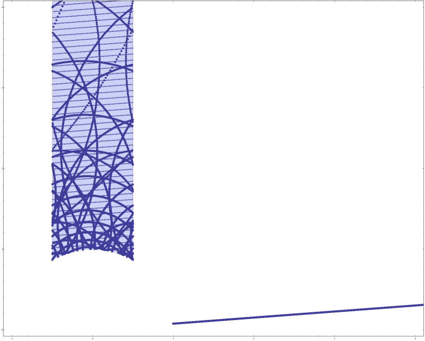
(a) Lattice case: $\Gamma=\operatorname{PSL}_{2}(\mathbb{Z})$

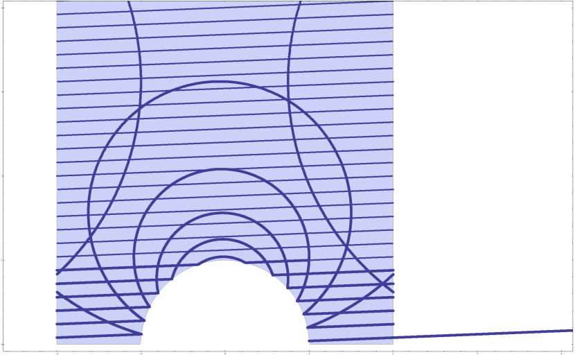
(b) Thin case: $\Gamma=\left\langle\bigl{(}\begin{smallmatrix}1&4\\ 0&1\end{smallmatrix}\bigr{)},\bigl{(}\begin{smallmatrix}0&-1\\ 1&0\end{smallmatrix}\bigr{)}\right\rangle$

Figure 1. A shear of the cuspidal geodesic ray

Our main equidistribution result is the following. Let $\Gamma$ be a discrete, Zariski-dense, geometrically finite subgroup of $G:=\operatorname{PSL}_{2}(\mathbb{R})$, and assume that the hyperbolic surface $\Gamma\backslash\mathbb{H}$, which may have finite or infinite volume, has at least one cusp. In particular, this forces the critical exponent $\delta$ of $\Gamma$ to exceed $1/2$; this will be our running assumption throughout.

The base point

$${\bf x}_{0}\in T^{1}(\Gamma\backslash\mathbb{H})\cong\Gamma\backslash G$$

in the unit tangent bundle determines the visual (under the forward geodesic flow) limit point $\mathfrak{a}$ on the boundary $\Gamma\backslash\partial\mathbb{H}$. We call the point ${\bf x}_{0}$, as well as its forward geodesic ray, ${\bf x}_{0}\cdot A^{+}$, cuspidal if $\mathfrak{a}$ is a cusp of $\Gamma$; here

$$A^{+}\ :=\ \{\bigl{(}\begin{smallmatrix}a&\\ &a^{-1}\end{smallmatrix}\bigr{)}:a>1\}.$$

(Note that we make no demands on the negative geodesic flow from ${\bf x}_{0}$.) Given such a ray, we define its shear (the ray is no longer geodesic), at time $T\in\mathbb{R}$, by:

$${\bf x}_{0}\cdot A^{+}\cdot\mathfrak{s}_{T}\ \subset\ \Gamma\backslash G,$$

where

$$\mathfrak{s}_{T}\ :=\ a_{1\over\sqrt{T^{2}+1}}n_{T},\qquad\qquad a_{y}\ =\ \bigl{(}\begin{smallmatrix}\sqrt{y}&\\ &1/\sqrt{y}\end{smallmatrix}\bigr{)},\quad n_{x}\ =\ \bigl{(}\begin{smallmatrix}1&x\\ &1\end{smallmatrix}\bigr{)}.$$ (1.1)

For example, if $\Gamma=\operatorname{SL}_{2}(\mathbb{Z})$, then the base point ${\bf x}_{0}=(i,\uparrow)$ has visual limit point $\mathfrak{a}=\infty$, and hence is cuspidal. The shear at time $T$ of the forward ray from ${\bf x}_{0}$, projected to $\Gamma\backslash\mathbb{H}$, is then simply the Euclidean ray $\{re^{i\theta}\}_{r>1}$, where $\cot\theta=T$. See Figure 1(a) for an illustration of this ray and its projection mod $\operatorname{PSL}_{2}(\mathbb{Z})$. Similarly, Figure 1(b) gives the same picture but for a thin group $\Gamma$.

We are interested in the behavior of such shears as $T\to\infty$ (and similarly for $T\to-\infty$). To this end, define the measure $\mu_{T}$ on a smooth, compactly supported observable $\Psi\in C^{\infty}_{0}(\Gamma\backslash G)$ by

$$\mu_{T}(\Psi)\ :=\ \int_{a\in A^{+}}\Psi({\bf x}_{0}\cdot a\cdot\mathfrak{s}_{T})da\ =\ \int_{1}^{\infty}\Psi({\bf x}_{0}\cdot a_{y}\cdot\mathfrak{s}_{T}){dy\over y}.$$ (1.2)

A slight simplification of our main result (see Theorem 3.2) is the following

Theorem 1.3.

Lattice Case: Assume that the quotient $\Gamma\backslash G$ has finite volume. Then there exists an $\eta>0$, depending on the spectral gap for $\Gamma$, so that

$$\mu_{T}(\Psi)\ =\ \log T\cdot\mu_{\Gamma\backslash G}(\Psi)+\mu_{\widetilde{Eis}}(\Psi)+O_{\Psi}\left(T^{-\eta}\right),$$ (1.4)

as $T\to\infty$. Here $\mu_{\Gamma\backslash G}$ is the probability Haar measure and $\mu_{\widetilde{Eis}}$ is a certain “regularized Eisenstein” distribution (see Remark 1.8 below).

Thin Case: Assume that $\Gamma$ is thin, that is, the quotient $\Gamma\backslash G$ has infinite volume. Then there exists an $\eta>0$, depending only on the critical exponent $\delta$ of $\Gamma$, and not on its spectral gap (!), so that

$$\mu_{T}(\Psi)\ =\ \mu_{{Eis}}(\Psi)+O_{\Psi}\left(T^{-\eta}\right),$$ (1.5)

as $T\to\infty$. Here $\mu_{Eis}$ is an (un-regularized) Eisenstein distribution.

Some comments are in order.

Remark 1.6.

For simplicity, we have stated Theorem 1.3 for compactly supported test functions $\Psi$, but our method applies just as well to a larger class of square-integrable functions with at least polynomial decay in the cusp $\mathfrak{a}$ (to ensure convergence of $\mu_{T}(\Psi)$); see §3.

Remark 1.7.

Throughout we make no attempt to optimize the various error exponents $\eta$, as can surely be done with a modicum of effort; our point is to illustrate a soft method which is powerful enough to obtain new results with power savings errors.

Remark 1.8.

Let us make the Eisenstein distributions arising in (1.4)–(1.5) less mysterious. These distributions are actually measures when $\Psi$ is right $K$-invariant; we restrict attention to this case to simplify the discussion below. First assume that $\Gamma$ is a lattice, that ${\bf x}_{0}=(i,\uparrow)$ with $\mathfrak{a}=\infty$ a cusp of $\Gamma$ of width $1$, and let $\Gamma_{\infty}=\bigl{(}\begin{smallmatrix}1&\mathbb{Z}\\ &1\end{smallmatrix}\bigr{)}$ be the isotropy group of $\mathfrak{a}$ in $\Gamma$. Then one has the standard Eisenstein series

$$E(z,s)\ :=\ \sum_{\gamma\in\Gamma_{\infty}\backslash\Gamma}{\mathfrak{Im}}(\gamma z)^{s},\qquad\qquad({\mathfrak{Re}}(s)>1),$$

which is well known [Sel56] to have meromorphic continuation and a simple pole at $s=1$ with residue $\operatorname{vol}(\Gamma\backslash\mathbb{H})^{-1}$. Thus the function

$$\widetilde{E}(z,s)\ :=\ E(z,s)\ -\ {1\over\operatorname{vol}(\Gamma\backslash\mathbb{H})\ (s-1)}$$ (1.9)

is regular at $s=1$; for example, when $\Gamma=\operatorname{PSL}_{2}(\mathbb{Z})$, we have (see, e.g., [IK04, (22.42), (22.63)–(22.69)])

$$\widetilde{E}(z,1)\ =\ {3\over\pi}\left(2\gamma-2{\zeta^{\prime}\over\zeta}(2)-\log(4y|\eta(z)|^{4})\right),\qquad$$ (1.10)

where $\gamma=0.577\cdots$ is Euler’s constant, $\zeta(s)$ is the Riemann zeta function, and $\eta(z)$ is the Dedekind eta function. Then the measure $\mu_{\widetilde{Eis}}$ is simply given by:

$$\mu_{\widetilde{Eis}}(\Psi)\ =\ \left\langle\Psi,\widetilde{E}(\cdot,1)\right\rangle_{\Gamma\backslash\mathbb{H}}.$$ (1.11)

Note that $\log|\eta(z)|$ grows like $y$ in the cusp, so $\mu_{\widetilde{Eis}}$ is also a non-finite measure. See (3.40) for the definition when $\Psi$ is not $K$-finite.

In the thin case of (1.5), the Eisenstein series is itself regular at $s=1$, that is, we can simply take $\widetilde{E}(z,s)=E(z,s)$; the spectral contribution is then all of lower order, so the power savings obtained in (1.5) is independent of any knowledge of a spectral gap for $\Gamma$.

Remark 1.12.

The first factor $\log T$ on the right side of (1.4) is a manifestation of the logarithmic divergence of the measure $\mu_{T}$. In the lattice case, a statement of the form

$$\mu_{T}(\Psi)\ =\ polynomial(\log T)\cdot\mu_{\Gamma\backslash G}(\Psi)\cdot\bigg{(}1\ +\ o(1)\bigg{)}$$ (1.13)

was suggested in work of Duke-Rudnick-Sarnak [DRS93, see below (1.4)]. Recently, Oh-Shah [OS14] used a purely dynamical method to prove (a variant of) (1.13) with a log-savings rate, that is, with $o(1)$ replaced by $O(1/\log T)$. With such a rate it is of course impossible to see the second-order main term (that is, the regularized Eisenstein distribution), and this identification will be key to some of our applications below. Moreover, it is hard to imagine how a quantity like (1.10) can be captured using only dynamics; our approach is quite different.

Before discussing the proof of Theorem 1.3, we first give some applications.

1.2. Application 1: Weighted Second Moments of $\operatorname{GL}(2)$ $L$-functions

Integrals like $\mu_{T}(\Psi)$ arise naturally in Sarnak’s approach (“changing the test vector”) [Sar85] for second moments of $L$-functions (see also, e.g., [Goo86, Ven10, MV10, DG10, DGG12]). We illustrate the method in the simplest case of a weight-$k$ holomorphic Hecke cusp form $f$ on $\operatorname{PSL}_{2}(\mathbb{Z})$, though the method works just as well for any $\operatorname{GL}(2)$ automorphic representation.

Write the Fourier expansion of $f$ as

$$f(z)=\sum_{n\geq 1}a_{f}(n)e(nz),$$

where $a_{f}(1)=1$ and the coefficients $a_{f}(n)$ are multiplicative, satisfying Hecke relations, and the Ramanujan bound $|a_{f}(p)|\leq 2p^{(k-1)/2}$ [Del74]. The standard $L$-function of $f$,

$$L(f,s)\ :=\ \sum_{n\geq 1}{a_{f}(n)\over n^{s+(k-1)/2}},$$

converges for ${\mathfrak{Re}}(s)>1$, has analytic continuation to $\mathbb{C}$, and a functional equation sending $s\mapsto 1-s$. The Rankin-Selberg $L$-function factors (see [Iwa97, (13.1)]) as

$$L(f\otimes\bar{f},s)\ :=\ \sum_{n\geq 1}{|a_{f}(n)|^{2}\over n^{s+(k-1)}}\ =\ {\zeta(s)\over\zeta(2s)}L(\operatorname{sym}^{2}f,s),$$

where $L(\operatorname{sym}^{2}f,s)$ is the symmetric square $L$-function, known [GJ78] to be the automorphic $L$-function of a cohomological form on $\operatorname{GL}(3)$.

A shear of the standard Hecke integral (already arising implicitly in classical work of Titchmarsch [Tit51, Chap. VII]) is the following calculation:

$$\int_{0}^{\infty}f\left(Ty+{iy}\right)y^{s+(k-1)/2}{dy\over y}=L(f,s)\mathcal{W}_{k}(s,T),$$ (1.14)

where

$$\mathcal{W}_{k}(s,T):=(2\pi)^{-(s+(k-1)/2)}\ \Gamma(s+\tfrac{k-1}{2})\ (1-iT)^{-(s+(k-1)/2)}.$$ (1.15)

Applying Parseval to (1.14) gives (for $s=1/2+it$)

$$\int_{0}^{\infty}\left|f\left(Ty+{iy}\right)\right|^{2}y^{k}{dy\over y}=\frac{1}{2\pi}\int_{\mathbb{R}}|L(f,\tfrac{1}{2}+it)|^{2}|\mathcal{W}_{k}(\tfrac{1}{2}+it,T)|^{2}dt.$$ (1.16)

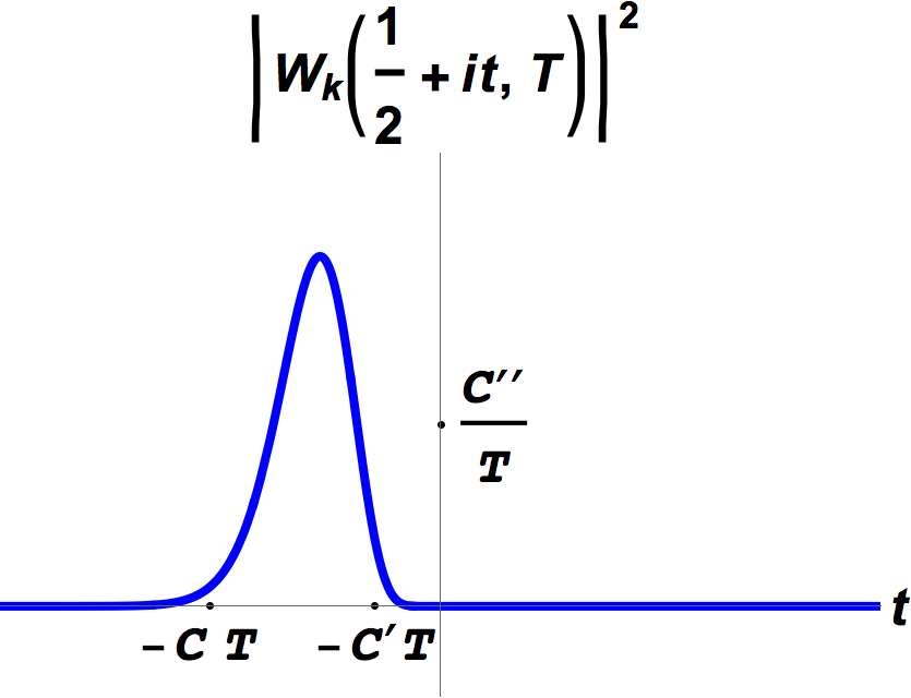
Figure 2. A sample graph of the smoothed archimedean weight $|\mathcal{W}_{k}(\tfrac{1}{2}+it,T)|^{2}$

A calculation with Stirling’s formula (or see Figure 2) shows that $|\mathcal{W}_{k}(\tfrac{1}{2}+it,T)|^{2}$ has rapid decay as soon as $|t|>T^{1+\varepsilon}$, and is of size roughly $1/T$ in the bulk. Thus the quantity on the right side of (1.16) behaves like a smoothed second moment of $L(f,s)$ on the critical line. Applying Theorem 1.3 with $\Psi=|f|^{2}y^{k}$ (and a little more work, see §4) gives the following.

Theorem 1.17.

With notation as above, there is an $\eta>0$ so that

$$\hskip-36.135pt\frac{1}{2\pi}\int_{\mathbb{R}}|L(f,\tfrac{1}{2}+it)|^{2}|\mathcal{W}_{k}(\tfrac{1}{2}+it,T)|^{2}dt$$

$$=\ 2{\|f\|^{2}\over\operatorname{vol}(\Gamma\backslash\mathbb{H})}\left(\log T\ +\ {\Lambda^{\prime}\over\Lambda}(\operatorname{sym}^{2}f,1)+\gamma-2{\zeta^{\prime}\over\zeta}(2)\right)\ +\ O_{f}(T^{-\eta}),$$

as $T\to\infty$. Here $\gamma$ is again Euler’s constant, $\|f\|$ is the Petersson norm, and $\Lambda^{\prime}/\Lambda$ is the logarithmic derivative of the completed symmetric-square $L$-function,

$$\Lambda(\operatorname{sym}^{2}f,s)\ =\ (4\pi)^{-(s+k-1)}\,\Gamma(s+k-1)\,L(\operatorname{sym}^{2}f,s).$$ (1.19)

Remark 1.20.

One can chase the various exponents in our proof to see that (1.17) holds with $\eta=1/14-\varepsilon$. Again, we are striving for simplicity of the method and not optimal exponents, see Remark 1.7. In fact, a straightforward refinement of the proof of Proposition 2.16 (using explicit spectral expansions in place of soft ergodic arguments) gives $\eta=16/39-\varepsilon$ on quoting the best-known bounds [KS03] towards the Ramanujan conjectures, and $\eta=1/2-\varepsilon$ conditionally. So in a sense, the proof of Theorem 1.17 is “sharp,” as there is no “loss” in the rate from a best-possible one.

Remark 1.21.

On comparing the lower order terms on the right hand side of (1.17) with the secondary term in (1.4), and using (1.10) and (1.11), one derives a Kronecker-type limit formula, in the form:

$${\left\langle\log(4y|\eta(z)|^{4}),|f|^{2}y^{k}\right\rangle\over\|f\|^{2}}\ =\ \gamma\ -\ {\Lambda^{\prime}\over\Lambda}(\operatorname{sym}^{2}f,1).$$ (1.22)

This identity is surely classical, though we were not able to locate a precise reference.

1.3. Application 2: Archimedean Counting for Orbits on Affine Quadrics

Another standard context where integrals like $\mu_{T}(\Psi)$ arise naturally is in the execution of certain Margulis/Duke-Rudnick-Sarnak/Eskin-McMullen type arguments [Mar04, DRS93, EM93] for counting discrete orbits on quadrics in archimedean balls. The setting is as follows.

Let $Q$ be a real ternary indefinite quadratic form (e.g., $Q({\bf x})=x^{2}+y^{2}-z^{2}$), fix $d\in\mathbb{R}$, and denote by $V=V_{Q,d}$ the affine quadric

$$V\ :\ Q=d.$$ (1.23)

The real points $V(\mathbb{R})$ enjoy an action by $G=\operatorname{SO}_{Q}^{\circ}(\mathbb{R})$, the connected component of the identity in the real special orthogonal group preserving $Q$. Let $\Gamma<G$ be a discrete, Zariski dense, geometrically finite subgroup of $G$, and assume, as throughout, that the critical exponent $\delta$ of $\Gamma$ exceeds $1/2$. Fix a base point ${\bf x}_{0}\in V(\mathbb{R})$, subject to the orbit

$$\mathcal{O}\ :=\ {\bf x}_{0}\cdot\Gamma\ \subset\ \mathbb{R}^{3}$$

being discrete.

For a fixed archimedean norm $\|\cdot\|$ on $\mathbb{R}^{3}$, let

$$B_{T}=\{{\bf x}\in\mathbb{R}^{3}:\|{\bf x}\|<T\}$$

be the norm ball of radius $T$. A very classical and well-studied problem is to give an effective (that is, with power savings error) estimate for

$$\mathcal{N}_{\mathcal{O}}(T)\ :=\ \left|\mathcal{O}\ \cap\ B_{T}\right|.$$

Despite the vast attention this problem has received over the years, there remained exactly two lacunary cases in which hitherto resisted solution; see §1.3.1 and Table 1 below for a detailed taxonomy of the situation. Equipped with Theorem 1.3, we can now resolve the outstanding cases.

Theorem 1.24.

There exist constants $C_{1},C_{2},$ and $\eta>0$ so that the following holds:

• If $\Gamma$ is a lattice in $G$, then

  $$\mathcal{N}_{\mathcal{O}}(T)\ =\ \big{(}C_{1}T\log T+C_{2}T\big{)}\big{(}1+O(T^{-\eta})\big{)}.$$ (1.25)

• If $\Gamma$ is thin, then

  $$\mathcal{N}_{\mathcal{O}}(T)\ =\ \big{(}C_{1}T+C_{2}T^{\delta}\big{)}\big{(}1+O(T^{-\eta})\big{)}.$$ (1.26)

Some comments are in order:

Remark 1.27.

1. All of the previously resolved cases of this problem (in the above generality) were such that the first term did not appear, that is, $C_{1}=0$ (whence $C_{2}>0$). Our new contributions are to the cases with $C_{1}>0$, which arise exactly when the stabilizer of ${\bf x}_{0}$ in $G$ is diagonalizable but “cuspidal” in $\Gamma\backslash G$; see §1.3.1 below.

2. If it happens that $\mathcal{O}$ is not just some arbitrary real discrete orbit but is actually the full integer quadric $V(\mathbb{Z})$ (assuming of course that the quadratic form $Q$ is rational and that $V(\mathbb{Z})$ is non-empty), then one has many more tools available to approach the counting problem for $\mathcal{N}_{\mathcal{O}}(T)$. Specifically, one can use, e.g., classical methods of exponential sums (see [Hoo63]), or half-integral weight automorphic forms, Poincaré series and shifted convolutions [Sar84, Blo08, TT13], or multiple Dirichlet series [HKKL13]. These give, when $\Gamma$ is a lattice and $C_{1}>0$, an estimate for $\mathcal{N}_{\mathcal{O}}(T)$ of the same strength as (1.25), that is, with a secondary main term and a power savings error. Such tools do not seem to apply to the general orbit counting problem.

3. In the thin case with $C_{1}>0$, the second term $C_{2}T^{\delta}$ is swamped by the error, and should not be confused with a lower order “main” term. We would like to acknowledge here that Nimish Shah suggested to us that the main term in this setting is of order $T$ rather than $T^{\delta}$; see also [OS13, Remark 1.7].

4. For the “new” cases with $C_{1}>0$, the exponent $\eta$ depends on the same quantities as in Theorem 1.3; that is, $\eta$ depends on the spectral gap in the lattice case, and only on the critical exponent in the thin case.

5. The constants $C_{1},C_{2}$ can be readily determined explicitly in terms of volumes, special values of (possibly regularized) Eisenstein series, and Patterson-Sullivan measures.

6. A consequence of Oh-Shah’s result discussed in Remark 1.12 gives, in the lattice case, the estimate (1.25), but with $O(T^{-\eta})$ replaced by the weaker error rate $O(1/(\log T)^{\eta})$ for some small $\eta>0$. This of course only identifies the first main term $C_{1}T\log T$, as the secondary term $C_{2}T$ is swallowed by the error.

1.3.1. Taxonomy

To explain the lacunary cases settled by Theorem 1.24, we begin by passing from $\operatorname{SO}_{Q}^{\circ}(\mathbb{R})$ to its spin cover $\operatorname{PSL}_{2}(\mathbb{R})\cong T^{1}(\mathbb{H}).$ Abusing notation, we continue to write $G$ and $\Gamma$ for their pre-images in $\operatorname{PSL}_{2}(\mathbb{R})$.

Let $H$ be the stabilizer of ${\bf x}_{0}$ in $G$,

$$H\ :=\ \{h\in G:{\bf x}_{0}\cdot h={\bf x}_{0}\},$$

and let

$$\Gamma_{H}:=\Gamma\cap H.$$

With ${\bf x}_{0}$ fixed, the norm $\|\cdot\|$ on $\mathbb{R}^{3}$ induces a left-$H$ invariant norm ${\left|\kern-1.07639pt\left|\kern-1.07639pt\left|\cdot\right|\kern-1.07639pt\right|\kern-1.07639pt\right|}$ on $G$ given by

$${\left|\kern-1.07639pt\left|\kern-1.07639pt\left|g\right|\kern-1.07639pt\right|\kern-1.07639pt\right|}=\|{\bf x}_{0}g\|.$$ (1.28)

We further abuse notation, writing $B_{T}$ for the left-$H$-invariant norm-$T$ ball in $G$, that is, $B_{T}\subset H\backslash G$. Then it is easy to see that

$$\mathcal{N}_{\mathcal{O}}(T)\ =\ |\Gamma_{H}\backslash\Gamma\ \cap\ B_{T}|.$$

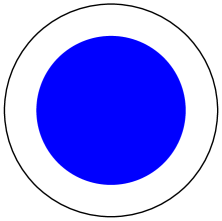
(a) Case $H\cong K$.

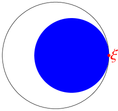
(b) Case $H\cong N$.

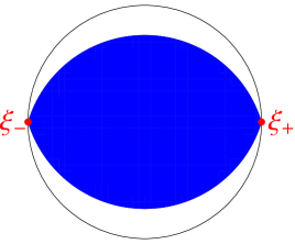
(c) Case $H\cong A$.

Figure 3. The region $B_{T}$ as a subset of the hyperbolic disk $\mathbb{D}$.

To investigate this counting problem more precisely, we illustrate the geometry of $B_{T}$, which is determined by whether the stabilizer $H$ is conjugate to the groups $K$, $N$, or $A$. That is, $H$ is either a maximal compact, a unipotent subgroup, or diagonalizable (over $\mathbb{R}$), and this corresponds to whether the real quadric $V(\mathbb{R})$ is a two-sheeted hyperboloid, a cone, or a one-sheeted hyperboloid, respectively. To visualize $B_{T}$ as a left-$H$-invariant subset of $G$, we project to the base space $\mathbb{H}$ (or alternatively, assume that the norm ${\left|\kern-1.07639pt\left|\kern-1.07639pt\left|\cdot\right|\kern-1.07639pt\right|\kern-1.07639pt\right|}$ is right-$K$-invariant), so that $B_{T}$ can be viewed as an $H$-invariant subset of the hyperbolic disk $\mathbb{D}\cong G/K$. Then $B_{T}$ is illustrated in Figure 3 in the three cases. Note that $B_{T}$ has zero, one, or two limit points (denoted $\xi$ or $\xi_{\pm}$) on the boundary $\partial\mathbb{D}$, corresponding to whether $H\cong K$, $H\cong N$, or $H\cong A$, respectively.

The asymptotic counting analysis depends in a fundamental way not only on whether $\Gamma$ is a lattice in $G$, but also on whether

$$\text{$\Gamma_{H}$ is a lattice in $H$}.$$ (1.29)

Lemma 1.30.

If (1.29) does not hold, then the discreteness of $\mathcal{O}$ is equivalent to the endpoints $\xi$ or $\xi_{\pm}$ of $H$ not being radial limit points for $\Gamma$.

This follows from a simple topological argument; we omit the proof. We decompose the analysis according to whether $\Gamma$ is a lattice or thin in $G$.

Case I: $\Gamma$ is a lattice.

Assuming that $\Gamma$ is a lattice in $G$, and also demanding that (1.29) holds, Duke-Rudnick-Sarnak [DRS93] and Eskin-McMullen [EM93] (see also [Mar04]) showed (in much greater generality than considered here) that there is some $\eta>0$ with

$$\mathcal{N}_{\mathcal{O}}(T)\ =\ {\operatorname{vol}_{H}(\Gamma_{H}\backslash H)\over\operatorname{vol}_{G}(\Gamma\backslash G)}\operatorname{vol}_{H\backslash G}(B_{T})\Bigg{(}1+O(T^{-\eta})\Bigg{)},$$ (1.31)

as $T\to\infty$. Here the volumes are taken to be compatible with choices of Haar measure on $G$, $H$, and $H\backslash G$. Note that $\operatorname{vol}_{H\backslash G}(B_{T})$ is of order $T$, so there is no logarithmic divergence in (1.31), that is, $C_{1}=0$ and $C_{2}>0$ in (1.25); see also Remark 1.27(1).

With Figure 3 and Lemma 1.30 in mind, we analyze separately the possible conjugacy classes of $H$.

• First if $H\cong K$ is compact, then (1.29) clearly holds automatically. In this case, the counting result (1.31) corresponds to counting in norm balls of $G$, which dates back to Delsarte [Del42], Huber [Hub56], and Selberg [Sel56].

• If $H\cong N$ is unipotent, then by Lemma 1.30, the boundary point $\xi$ of $H$ must be a cusp. That is, $\Gamma_{H}\backslash H$ is a closed horocycle, so $\Gamma_{H}$ is a lattice in $H$, and (1.29) is again automatically satisfied. In this case, the count takes place in a strip $\Gamma_{H}\backslash G$, and the equidistribution of low-lying closed horocycles [Mar04, Zag81, Sar81] can be used to establish (1.31).

• Lastly, if $H\cong A$ is diagonalizable (over $\mathbb{R}$), then Lemma 1.30 forces one of two settings. Either

  $(i)$: $\Gamma_{H}$ is a lattice in $H$, whence $\Gamma_{H}\backslash H$ corresponds to a closed geodesic on $\Gamma\backslash G$. Then (1.29) holds, so (1.31) follows from [DRS93]. Or

  $(ii)$: $\Gamma_{H}$ is finite, but both limit points $\xi_{+}$ and $\xi_{-}$ of $H$ (see Figure 3(c)) are cusps of $\Gamma$. Here we are in the diagonalizable but “cuspidal” setting referred to in Remark 1.27(1). This case is the only one (when $\Gamma$ is a lattice in $G$) not satisfying (1.29) despite the discreteness of the orbit $\mathcal{O}$; it is precisely the new case settled by Theorem 1.24.

Case II: $\Gamma$ is thin.

In this setting, we again decompose the problem of estimating $\mathcal{N}_{\mathcal{O}}(T)$ into separate cases, depending on the conjugacy class of $H$, and on whether condition (1.29) holds (there are now more situations in which $\mathcal{O}$ is discrete but (1.29) can fail).

• When $H\cong K$ is compact, the condition (1.29) is again automatically satisfied, and in this case Lax-Phillips [LP82] showed that

  $$\mathcal{N}_{\mathcal{O}}(T)=C_{2}\,T^{\delta}\Bigg{(}1+O(T^{-\eta})\Bigg{)},$$ (1.32)

  where $\eta>0$ depends on the spectral gap for $\Gamma$. This corresponds to the case $C_{1}=0$ in (1.26); again, see Remark 1.27(1).

• If $H\cong N$ is unipotent, the discreteness of $\mathcal{O}$ forces one of two cases. Either

  (i) $\Gamma_{H}$ is a lattice in $H$, so (1.29) holds, and $\Gamma_{H}\backslash H$ corresponds to a closed horocycle. In this case, the asymptotic formula is (1.32) was shown in the second-named author’s thesis [Kon09]. Or

  (ii) $\Gamma_{H}$ is trivial, whence Lemma 1.30 forces the limit point $\xi$ of $H$ to be in the free boundary, that is, it is not in the limit set of $\Gamma$. The asymptotic here is also of the form (1.32); see [KO12].

• Finally, when $H\cong A$ is diagonalizable, there are three separate cases to consider. The discreteness of $\mathcal{O}$ now implies either

  (i) $\Gamma_{H}$ is a lattice in $H$, again corresponding to a closed geodesic on $\Gamma\backslash G$. Then the same asymptotic (1.32) follows from now-standard methods using the equidistribution result of Bourgain-Kontorovich-Sarnak [BKS10]. Or

  (ii) $\Gamma_{H}$ is thin in $H$, in which case each of the two endpoints $\xi_{\pm}$ of $H$ is either a cusp of $\Gamma$ or in the free boundary. If

  (a) both endpoints $\xi_{\pm}$ are in the free boundary, then the methods of [BKS10] can again be used to show the same asymptotic (1.32). (The key is that only a finite portion of the sheared geodesic ray interacts with the limit set – see [KO12] where a similar phenomenon was studied in the case of a unipotent stabilizer.) Otherwise,

  (b) at least one of $\xi_{\pm}$ is a cusp of $\Gamma$. This is the other new lacunary case of Theorem 1.24, and is the only thin case for which (1.26) has $C_{1}>0$. Note that if one boundary point is a cusp and the other is in the free boundary, the former has contribution of order $T$, while the latter’s contribution, of order $T^{\delta}$, is dominated by the former’s error term.

This concludes our taxonomy. To summarize, the following table serves to illustrate that Theorem 1.24 above completes the effective solution to the general counting orbital problem in our context:

	$N$	$A$	$K$
(lattice, lattice)	[Zag81, Sar81]	[DRS93, EM93]	[Del42, Hub56, Sel56]
(lattice, thin)	impossible by discreteness of $\mathcal{O}$	“lacunary” case settled in (1.25)	impossible by compactness of $K$
(thin, lattice)	[Kon09]	[BKS10]	[LP82]
(thin, thin)	[KO12]	$\begin{cases}\text{\cite[cite]{[\@@bibref{}{BourgainKontorovichSarnak2010}{}{}]},}&\text{if both $\xi_{\pm}\notin\Lambda$, }\\ \pagecolor{pink}{\hskip-7.22743pt\begin{tabular}[]{c}``lacunary'' case\\ settled in \eqref{eq:countThin},\end{tabular}}&\text{ otherwise, }\end{cases}$	impossible by compactness of $K$

Table 1. The new cases of Theorem 1.24, highlighted, are those with $C_{1}>0$.

Remark 1.33.

When the critical exponent $\delta\leq 1/2$, work of Naud [Nau05], extending Dolgopyat’s methods [Dol98], allows one to conclude, in the cases not excluded by Lemma 1.30, an effective asymptotic of the form (1.32). So the lacunary cases do not occur here, as there are no cusps (and hence no cuspidal geodesic rays) when $\delta\leq 1/2$.

Remark 1.34.

As pointed out in [OS14, p. 917] (at least for $\Gamma$ a lattice), the only lacunary cases in the more general setting of $Q$ having signature $(n,m)$ are precisely those of signature $(2,1)$, that is, those considered here; so we have lost no generality in restricting to $\operatorname{PSL}_{2}(\mathbb{R})$. This is because the stabilizer $H$ is either unipotent, compact, or fixes a form of signature $(n-1,m)$ or $(n,m-1)$. The only non-compact such not generated by unipotents has signature $(1,1)$, whence $Q$ has signature $(2,1)$.

1.4. Surprise: Non-equidistribution in Congruence Cosets!

The most unexpected consequence of Theorem 1.24 comes from studying the thin case in cosets of congruence towers, as we now describe. Assume that $Q$ is not just a real quadratic form but an integral one, and that $\Gamma$ is a subgroup of the integral special orthogonal group

$$\Gamma\ <\ \operatorname{SO}_{Q}(\mathbb{Z}).$$

Given an integer $q\geq 1$, we can then form the level-$q$ “congruence” subgroups $\Gamma(q)<\Gamma$, defined as

$$\Gamma(q)\ :=\ \ker(\Gamma\to\operatorname{SO}_{Q}(\mathbb{Z}/q\mathbb{Z})).$$

For many applications, one wishes to study the same counting problem as above, with the orbit $\mathcal{O}={\bf x}_{0}\cdot\Gamma$ replaced by the congruence orbit ${\bf x}_{0}\cdot\Gamma(q)$, or better yet, by some “congruence coset” orbit,

$$\mathcal{O}_{q,\varpi}\ :=\ {\bf x}_{0}\cdot\varpi\cdot\Gamma(q),$$

for a given $\varpi\in\Gamma/\Gamma(q)$. Let

$$\mathcal{N}_{q,\varpi}(T)\ :=\ |\mathcal{O}_{q,\varpi}\ \cap\ B_{T}|$$

be the corresponding counting function, which we wish to estimate uniformly with $q$ and $T$ (and $\varpi$) varying in some allowable range.

Theorem 1.24 applies just as well to estimate $\mathcal{N}_{q,\varpi}(T)$, and in all previously studied examples, the asymptotic analysis showed that

$$\mathcal{N}_{q,\varpi}(T)\ \sim\ \frac{1}{[\Gamma:\Gamma(q)]}\mathcal{N}_{\mathcal{O}}(T),\qquad\qquad\qquad(T\to\infty),$$ (1.35)

that is, the asymptotic is independent of $\varpi$, so the orbits are equidistributed among congruence cosets. (Moreover, (1.35) even holds with $q$ allowed to grow sufficiently slowly with $T$.) This equidistribution is a key input, for example, in executing an Affine Sieve in an archimedean ordering (see, e.g., [Kon09, NS10, LS10, BGS11, KO12, MO13, BK14, HK14]). An analysis of Theorem 1.24 shows that, for thin orbits, there are cosets which are not uniformly distributed in archimedean balls!

Proposition 1.36.

Assume that $\Gamma$ is thin, and that the orbit $\mathcal{O}$ is has diagonalizable and cuspidal stabilizer, that is, $C_{1}>0$ in (1.26). Then the equidistribution (1.35) in congruence cosets is false. For example, for each fixed $q$, there is some $\varpi\in\Gamma/\Gamma(q)$ so that

$$\mathcal{N}_{q,\varpi}(T)\ \gg\ \frac{1}{q}\ T,$$ (1.37)

while

$$\frac{1}{[\Gamma:\Gamma(q)]}\mathcal{N}_{\mathcal{O}}(T)\ \ll\ \frac{1}{q^{3}}\ T,$$

as $T\to\infty$. (The implied constants above may depend on $\Gamma$ and ${\bf x}_{0}$, but obviously not on $q$ or $T$.)

This means that the standard Affine Sieve procedure cannot be executed in this ordering. (Note that the case considered in Proposition 1.36 is precisely the one omitted in the sieving statement [MO13, Cor 1.19].)

1.5. Outline of the Proofs and Paper

Our proof of Theorem 1.3 is surprisingly simple, and proceeds in two stages. The first is to show that $\mu_{T}(\Psi)$ in some sense equidistributes in the “strip $\Gamma_{\infty}\backslash\mathbb{H}$”, but with respect to $dx\,dy/y$, as opposed to Haar measure $dx\,dy/y^{2}$ (for a hint of this, look again at Figure 1); this fact uses only the decay of the Fourier coefficients of $\Psi$ (itself a simple consequence of mixing via low-lying horocycles; see Proposition 2.16). Then stage two is to relate this equidistribution to Eisenstein series, where we mimic Sarnak’s approach in [Sar81, Zag81] to conclude the proof.

The rest of the paper proceeds as follows. In §2, we set notation and recall basic facts needed through the paper. Then in §3, we prove the main equidistribution result, Theorem 1.3, and its generalization (Theorem 3.2). Then Theorem 1.17 is proved in §4 using the Rankin-Selberg “unfolding” technique. Finally, Theorem 1.24 and Proposition 1.36 are proved in §5.

1.6. Notation

Constants $0<C<\infty$ and $0<\eta<1$ can change from line to line, and $\varepsilon>0$ represents an arbitrarily small quantity. The transpose of a matrix $g$ is written ${}^{\top}\!g$. Unless otherwise specified, implied constants depend at most on $\Gamma$, which is treated as fixed. The symbol ${\bf 1}_{\{\cdot\}}$ represents the indicator function of the event $\{\cdot\}$.

Acknowledgements

The authors would like to express their gratitude to Jens Marklof, Curt McMullen, and Peter Sarnak for many enlightening comments and suggestions. The second author would especially like to thank Valentin Blomer, Farrell Brumley, and Nicolas Templier for many hours of discussion about this problem; see also the related work in [BBKT14].

2. Preliminaries

In this section, we set all notation and basic facts used throughout.

2.1. Hyperbolic Geometry

Let $\mathbb{H}:=\{z\in\mathbb{C}:{\mathfrak{Im}}z>0\}$ denote the hyperbolic upper half-plane. At each point $z\in\mathbb{H}$, and tangent vector $\zeta\in T_{z}\mathbb{H}\cong\mathbb{C}$, the Riemannian structure is $\|\zeta\|_{z}:=|\zeta|/{\mathfrak{Im}}z.$ The unit tangent bundle $T^{1}\mathbb{H}$ is then

$$T^{1}\mathbb{H}\ :=\ \{(z,\zeta)\in\mathbb{H}\times\mathbb{C}:\|\zeta\|_{z}=1\}.$$

The group $G=\operatorname{PSL}_{2}(\mathbb{R})$ acts on $T^{1}\mathbb{H}$ via

$$\left(\begin{array}[]{cc}a&b\\ c&d\end{array}\right)\ :\ (z,\zeta)\mapsto\left({az+b\over cz+d},{\zeta\over(cz+d)^{2}}\right),$$

and moreover we can identify $G\cong T^{1}\mathbb{H}$ under $g\mapsto g(i,\uparrow)$. We also use the disk model $\mathbb{D}:=\{z\in\mathbb{C}:|z|<1\},$ identified with $\mathbb{H}$ under the map

$$\mathbb{H}\ni z\ \mapsto\ (z-i)/(z+i)\in\mathbb{D}.$$

Let $\Gamma$ be a finitely generated, Zariski dense, discrete subgroup of $G$. As above, we identify $T^{1}(\Gamma\backslash\mathbb{H})\cong\Gamma\backslash G$. For a fixed base point $\mathfrak{o}\in\mathbb{H}$, the critical exponent

$$\delta=\delta(\Gamma)\ \in\ [0,1]$$

of $\Gamma$ is the abscissa of convergence of the Poincaré series

$$\sum_{\gamma\in\Gamma}\exp(-sd(\gamma\mathfrak{o},\mathfrak{o})),\hskip 72.26999pt({\mathfrak{Re}}(s)>\delta).$$

Here $d(\cdot,\cdot)$ is hyperbolic distance, and $\delta$ does not depend on the choice of $\mathfrak{o}$. Let $dg$ be a choice of Haar measure on $G$; we call $\Gamma$ a lattice if $\Gamma\backslash G$ has finite measure, and thin otherwise. This is measured by the critical exponent $\delta$, as $\delta=1$ or $\delta<1$ exactly when $\Gamma$ is a lattice or thin, respectively [Pat76]; the Zariski-density of $\Gamma$ implies that $\delta>0$. The limit set

$$\Lambda=\Lambda(\Gamma)\ \subset\ \partial\mathbb{H}\cong S^{1}\cong\mathbb{R}\sqcup\{\infty\}$$

of $\Gamma$ is the set of limit points of $\gamma\mathfrak{o}$, $\gamma\in\Gamma$; it also does not depend on the choice of $\mathfrak{o}$. The Hausdorff dimension of $\Lambda$ is exactly equal to the critical exponent $\delta$ [Pat76, Sul84]. A boundary point $\xi\in\partial\mathbb{H}$ is a cusp of $\Gamma$ if it is the fixed point of a parabolic element in $\Gamma$; these all lie in the limit set $\Lambda$, and we let $\Lambda_{cusp}$ denote the subset of cusps. A limit point $\xi\in\Lambda$ is called radial (or a “point of approximation”) if there is a sequence $\{\gamma_{n}\mathfrak{o}\}$, $\gamma_{n}\in\Gamma$, which stays a bounded distance away from a geodesic ray ending at $\xi$. Let $\Lambda_{rad}$ denote the set of radial limit points; it is a basic fact [Bea83] that the limit set decomposes disjointly into radial and cuspidal points,

$$\Lambda\ =\ \Lambda_{cusp}\sqcup\Lambda_{rad}.$$

The complement of the limit set in $\partial\mathbb{H}$ is called the free boundary of $\Gamma$,

$$\mathcal{F}=\mathcal{F}(\Gamma)\ :=\ \partial\mathbb{H}\setminus\Lambda,$$

and $\mathcal{F}=\O$ if and only if $\Gamma$ is a lattice. We record here the decomposition

$$\partial\mathbb{H}\ =\ \mathcal{F}\sqcup\Lambda_{cusp}\sqcup\Lambda_{rad}.$$ (2.1)

We assume henceforth that $\Gamma$ has at least one cusp, whence its critical exponent exceeds $1/2$,

$$\delta\ >\ 1/2.$$ (2.2)

2.2. Spectral Theory

The hyperbolic Laplace operator $\Delta:=-y^{2}(\partial_{xx}+\partial_{yy})$ acts (after unique extension) on the space $L^{2}(\Gamma\backslash\mathbb{H})$ of square-integrable automorphic functions, and is self-adjoint and positive semi-definite. Let $\Omega=\Omega(\Gamma)\subset[0,\infty)$ denote the spectrum of $\Delta$. The assumption that $\Gamma$ has at least one cusp implies the existence of continuous spectrum above $1/4$, that is, $[1/4,\infty)\subset\Omega$ (there may also be embedded discrete spectrum in this range, which only occurs when $\Gamma$ is a lattice [Sel56, Pat75]). Below $1/4$ the spectrum is finite [LP82] and nonempty (by (2.2)); we denote these eigenvalues, often referred to as the “exceptional spectrum,” by

$$0\leq\lambda_{0}<\lambda_{1}\leq\cdots\leq\lambda_{max}<\frac{1}{4},$$

and introduce spectral parameters $1/2<s_{j}\leq 1$ defined by

$$\lambda_{j}\ =\ s_{j}(1-s_{j}),$$

so that

$$1\geq s_{0}>s_{1}\geq\cdots\geq s_{max}>\frac{1}{2}.$$ (2.3)

The bottom eigenvalue $\lambda_{0}$ is simple, and is related to the geometry of $\Lambda$ via the Patterson-Sullivan formula [Pat76, Sul84]

$$\lambda_{0}\ =\ \delta(1-\delta),$$

that is, $s_{0}=\delta$.

2.3. Algebra

We will use standard notation for the subgroups $N$, $A$, and $K$ of $G$, given by:

$$N:=\left(\begin{array}[]{cc}1&\mathbb{R}\\ 0&1\end{array}\right),\quad A:=\left\{\operatorname{diag}(a,1/a):a>0\right\},\quad K:=\operatorname{SO}(2),$$ (2.4)

and containing typical elements

$$n_{x}:=\left(\begin{array}[]{cc}1&x\\ &1\end{array}\right),\quad a_{y}:=\left(\begin{array}[]{cc}\sqrt{y}&\\ &1/\sqrt{y}\end{array}\right),\quad k_{\theta}=\left(\begin{array}[]{cc}\cos\theta&\sin\theta\\ -\sin\theta&\cos\theta\end{array}\right).$$

As right actions, they correspond, respectively, to the unipotent flow, geodesic flow, and rotation of the tangent vector, keeping the base point fixed. On the other hand, as left actions, the correspond, respectively, to horizontal translation, scaling, and motion around a hyperbolic circle centered at $i$. Haar measure $dg$ in Iwasawa coordinates $g=n_{x}a_{y}k_{\theta}$ is then given by $dg=dx\,y^{-2}dy\,d\theta$. The right-action by the semigroup $A^{+}:=\{a_{y}:y>1\}$ corresponds to the positive geodesic flow, so that a given point ${\bf x}_{0}\in G\cong T^{1}\mathbb{H}$ gives rise to the geodesic ray ${\bf x}_{0}A^{+}$.

2.4. Representation Theory

By the Duality Theorem [GGPS66], the spectral decomposition (2.3) corresponds to the decomposition of the right regular representation of $G$ on $L^{2}(\Gamma\backslash G)$ as

$$L^{2}(\Gamma\backslash G)\ =\ V_{0}\oplus V_{1}\oplus\cdots\oplus V_{max}\oplus V_{temp}.$$

Here $V_{temp}$ consists of the tempered spectrum (a reducible subspace); each $V_{j}$, $j=1,\dots,max$ is an irreducible complementary series representation of parameter $s_{j}$; and $V_{0}$ is either the trivial representation (if $\Gamma$ is a lattice), or a complementary series representation of parameter $s_{0}=\delta$ (if $\Gamma$ is thin).

We record here a Sobolev-norm version [BR98] of the exponential decay of matrix coefficients. Fix a basis $\mathscr{B}=\{X_{1},X_{2},X_{3}\}$ for the Lie algebra $\mathfrak{g}$ of $G$, and given a smooth test function $\Psi\in C^{\infty}(\Gamma\backslash G)$, define the “$L^{p}$, order-$d$” Sobolev norm $\mathcal{S}_{p,d}(\Psi)$ as

$$\mathcal{S}_{p,d}(\Psi)\ :=\ \sum_{\operatorname{ord}(\mathscr{D})\leq d}\|\mathscr{D}\Psi\|_{L^{p}(\Gamma\backslash G)}.$$

Here $\mathscr{D}$ ranges over monomials in $\mathscr{B}$ of order at most $d$.

Theorem 2.5 ([CHH88, Sha00, Ven10]).

Let $(\pi,V)$ be a unitary $G$-representation, and assume there is a number $\Theta>1/2$ so that $V$ does not weakly contain any complementary series with parameter $s>\Theta$. Then for all smooth $v,w\in V^{\infty}$, we have

$$|\left\langle\pi(g).v,w\right\rangle|\ \ll\ \|g\|^{2(1-\Theta)}\mathcal{S}_{2,1}(v)\mathcal{S}_{2,1}(w),$$ (2.6)

as $\|g\|^{2}:=\operatorname{tr}(g\,{}^{\top}\!g)\to\infty$. The implied constant is absolute.

Later we will encounter other Sobolev norms which are convex combinations of those above.

2.5. Uniform Spectral Gaps

Recalling the spectral decomposition (2.3), we call a number $\Theta\in(1/2,\delta)$ a spectral gap for $\Gamma$ if $\Theta>s_{1}$. To make sense of a uniform such gap, we assume integrality. As in §1.4, if $\Gamma$ consists of integer matrices, $\Gamma<\operatorname{PSL}_{2}(\mathbb{Z})$, we may, given an integer $q\geq 1$, define the level-$q$ “congruence” subgroup

$$\Gamma(q)\ :=\ \ker(\Gamma\to\operatorname{PSL}_{2}(\mathbb{Z}/q\mathbb{Z})).$$

Let $\Omega(q)$ be the spectrum of $\Delta$ on $L^{2}(\Gamma(q)\backslash\mathbb{H})$; clearly $\Omega\subset\Omega(q)$, and in general this inclusion is strict. We will call a number $\Theta\in(1/2,\delta)$ a uniform spectral gap for $\Gamma$ if, for all $q\geq 1$,

$$\Omega(q)\cap(\delta(1-\delta),\Theta(1-\Theta)]\ =\ \O,$$ (2.7)

that is, there are no eigenvalues at any level $q$ in a neighborhood of the base eigenvalue $\lambda_{0}=\delta(1-\delta)$. (Note that this definition is different from other related definitions in the literature.) In a number of statements below, several quantities depend on the spectral gap in the lattice case, but only on the critical exponent in the thin case; to unify the two notions, we will say that such quantities depend on the first non-zero eigenvalue of $\Gamma$.

2.6. Eisenstein Series

In this section we recall some basic facts from the theory of Eisenstein series. We will assume here that the Eisenstein series is with respect to a cusp at $\infty$ and note that Eisenstein series corresponding to other cusps are defined similarly, after conjugating that cusp to $\infty$. In our applications, we will not have the flexibility to demand the cusp have width $1$, so deal below with arbitrary width.

The Eisenstein series corresponding to a cusp at $\infty$ of width $\omega>0$ is defined in the half-plane ${\mathfrak{Re}}(s)>1$ by the convergent series

$$E(z,s)\ :=\ \frac{1}{\omega}\!\sum_{\gamma\in\Gamma_{\infty}\backslash\Gamma}{\mathfrak{Im}}(\gamma z)^{s},$$ (2.8)

where $\Gamma_{\infty}=\left(\begin{smallmatrix}1&\omega\mathbb{Z}\\ 0&1\end{smallmatrix}\right)$.

Assume first that $\Gamma$ is a lattice. Then $E(z,s)$ has a meromorphic continuation to $\mathbb{C}$ with a functional equation sending $s\mapsto 1-s$. In fact, it is analytic in the half plane ${\mathfrak{Re}}(s)>1/2$ except for a simple pole at $s=1$ and perhaps finitely many poles

$$1>\sigma_{1}\geq\cdots\geq\sigma_{h}>1/2.$$ (2.9)

These poles comprise the “residual spectrum,” which is a subset of the “exceptional spectrum” in (2.3); the remaining spectrum in this range, if any, is cuspidal. The residue at $s=1$ is

$$\operatorname{Res}_{s=1}E(s,z)={1\over\operatorname{vol}(\Gamma\backslash\mathbb{H})}$$

and

$$\varphi_{\sigma_{j}}(z)=\operatorname{Res}_{s=\sigma_{j}}E(s,z)$$

are the residual forms.

For any integer $n\in\mathbb{Z}$ we also define the weight $2n$ Eisenstein series by

$$E_{n}(z,s)\ :=\ \frac{1}{\omega}\!\sum_{\gamma\in\Gamma_{\infty}\backslash\Gamma}{\mathfrak{Im}}(\gamma z)^{s}\epsilon_{\gamma}(z)^{2n},$$ (2.10)

where

$$\epsilon_{g}(z)={cz+d\over|cz+d|},\qquad g=\left(\begin{array}[]{cc}a&b\\ c&d\end{array}\right).$$

Unless the weight $n=0$, the $E_{n}$’s are all regular at $s=1$, that is, $E_{0}=E$ is the only Eisenstein series with a pole at $s=1$. In the range $\tfrac{1}{2}<{\mathfrak{Re}}(s)<1$, the poles of $E_{n}$ are the same $s=\sigma_{1},\dots,\sigma_{h}$ as those of $E$. For each such pole $\sigma=\sigma_{j}$ we denote by

$$\varphi_{\sigma,n}=\operatorname{Res}_{s=\sigma}E_{n}(z,s),$$ (2.11)

the (un-normalized) residual form of weight $2n$.

We note for future reference that the weight-$2n$ Eisenstein series and the weight-$2n$ residual forms all lie in the space $(\Gamma,2n)$ of functions on $\mathbb{H}$ transforming by

$$f(\gamma z)=\epsilon_{\gamma}(z)^{2n}f(z).$$ (2.12)

Still assuming that $\Gamma$ is a lattice, we also have the following bounds coming from the spectral decomposition of $L^{2}(\Gamma\backslash G)$, see, e.g. [Iwa97]. For any square-integrable $f\in(\Gamma,2n)$, we have the bound

$$\frac{1}{2\pi}\int_{\mathbb{R}}|\left\langle f,E_{n}(\cdot,\tfrac{1}{2}+ir)\right\rangle|^{2}dr\leq\left\|f\right\|_{2}^{2}.$$ (2.13)

When $\Gamma$ is thin, we will only use the fact that the defining series in (2.8) and (2.10) converge absolutely in the range ${\mathfrak{Re}}(s)>\delta$.

2.7. Decay of Fourier Coefficients

In this subsection we wish to record the basic fact that the (parabolic) Fourier coefficients of an automorphic function decay in the cusp, in a uniform sense. The method we use to establish this is completely standard, though the requisite uniformity does not seem to be in the literature; hence we give sketches of proofs for the reader’s convenience. We again assume that $\Gamma$ has a cusp at $\infty$ of width $\omega>0$, that is, the isotropy group $\Gamma_{\infty}$ of $\infty$ is generated by the translation $z\mapsto z+\omega$.

Then a smooth, square-integrable, $\Gamma$-automorphic function $\Psi\in L^{2}\cap C^{\infty}(T^{1}(\Gamma\backslash\mathbb{H}))$ has a Fourier expansion:

$$\Psi(x+iy,\zeta)\ =\ \sum_{m\in\mathbb{Z}}a_{\Psi}(m;y,\zeta)\ e_{\omega}(mx),$$ (2.14)

where $e_{\omega}(x):=e^{2\pi ix/\omega}$, and the Fourier coefficients are given by

$$a_{\Psi}(m;y,\zeta)\ :=\ \frac{1}{\omega}\int_{0}^{\omega}\Psi(x+iy,\zeta)e_{\omega}(-mx)dx.$$ (2.15)

The next proposition records the decay of such as $y\to 0$ (in a uniform statement); the subscripts $F$ below stand for “Fourier coefficients.”

Proposition 2.16.

There is a “Sobolev” norm $\mathcal{S}_{F}(\Psi)$ and constants $0<C_{F}<\infty$ and $0<\alpha_{F}<1$, so that, uniformly over all $y>0$ and $m\in\mathbb{Z}\setminus\{0\}$, we have

$$\left|a_{\Psi}(m;y,\zeta)\right|\ll\mathcal{S}_{F}(\Psi)\ |m|^{C_{F}}\ y^{\alpha_{F}}.$$ (2.17)

The constants $\alpha_{F}$ and $C_{F}$ depend on the first non-zero eigenvalue of $\Gamma$.

The Sobolev norm and exact values of the constants $C_{F}$ and $\alpha_{F}$ are given below in (2.23), (2.24), and (2.25), respectively; the last claim of the proposition is then clear, namely, that the constants depend on the spectral gap when $\Gamma$ is a lattice, and only on the critical exponent when $\Gamma$ is thin. As we are not striving for optimal exponents (recall Remark 1.7), we have chosen to suppress their precise values so as not to clutter the presentation. Recall also our convention that implied constants may depend at most on $\Gamma$, unless stated otherwise.

The Proposition is an easy consequence of another standard fact, namely the equidistribution of (pieces of) “low-lying” horocycles; the subscripts $H$ below stand for “Horocycle pieces.”

Proposition 2.18.

There is a “Sobolev” norm $\mathcal{S}_{H}(\Psi)$ and constants $C_{H}<\infty$ and $0<\alpha_{H}<1$, so that, uniformly over all $y>0$ and open intervals $\mathcal{I}\subset(0,\omega)$, we have

$$\frac{1}{|\mathcal{I}|}\int_{\mathcal{I}}\Psi(x+iy,\zeta)dx\ =\ {1\over\operatorname{vol}(\Gamma\backslash G)}\int_{\Gamma\backslash G}\Psi\ dg+O\Bigg{(}\mathcal{S}_{H}(\Psi)\ |\mathcal{I}|^{-C_{H}}\ y^{\alpha_{H}}\Bigg{)}.$$ (2.19)

This statement holds whether $\Gamma$ is a lattice or not, with the interpretation that the first term on the right-hand-side of (2.19) vanishes in the thin case. The constants $C_{H}$ and $\alpha_{H}$ depend on the first non-zero eigenvalue of $\Gamma$.

Again, the norm and constants are detailed in (2.20), (2.21), and (2.22), which we have suppressed in the interest of exposition. Much stronger versions of (2.19) exist in the literature (at least in the lattice case, for which see, e.g., [Str04, SU15]), but for the reader’s convenience, we provide a quick

Proof of Proposition 2.18 [Sketch].

We may assume that $y<1$ (for the statement is obviously true otherwise), and we may moreover assume that $\Psi$ is right-$K$-invariant (or replace $\Psi$ by $\tilde{\Psi}:=\pi(k_{\theta}^{-1})\Psi$, where $2\theta$ is the angle of $\zeta$ measured counterclockwise from the vertical). Then the left hand side of (2.19) is

$$\mathscr{M}\ :=\ \frac{1}{|\mathcal{I}|}\int_{x\in\mathcal{I}}\Psi(n_{x}a_{y})dx.$$

Let $\rho$ be a smooth, non-negative function on $\mathbb{R}$ with support in $[-1,1]$ and $\int_{\mathbb{R}}\rho=1$. For $\eta>0$ to be chosen later, concentrate $\rho$ to $\rho_{\eta}(x):=\eta^{-1}\rho(x/\eta)$. Write $\overline{N}:={}^{\top}\!N$, $\overline{n}_{x}:={}^{\top}\!n_{x}$ for the opposite horocyclic group and element. Then the multiplication map

$$N\times A\times\overline{N}\ \to\ G\ :\ (n,a,\overline{n})\mapsto na\overline{n}$$

is bijective on an open neighborhood of the origin. Define $\xi:G\to\mathbb{R}_{\geq 0}$, supported in such a neighborhood, via:

$$\xi(n_{x}a_{t}\overline{n}_{s})\ :=\ c_{\xi}\cdot\left(\rho_{\eta}\star\frac{1}{|\mathcal{I}|}{\bf 1}_{\mathcal{I}}\right)\!(x)\cdot\rho_{\eta}(\log t)\cdot\rho_{\eta}(s),$$

where $\star$ denotes convolution, and $c_{\xi}\asymp 1$ is a constant (independent of $\eta$) chosen so that $\int_{G}\xi=1$. Automorphize $\xi$ to

$$\Xi(g)\ :=\ \sum_{\gamma\in\Gamma}\xi(\gamma g),$$

which is a function on $\Gamma\backslash G$ with $\int_{\Gamma\backslash G}\Xi=1$. Finally, consider the matrix coefficient:

$$\mathscr{C}\ :=\ \left\langle\pi(a_{y}).\Psi,\Xi\right\rangle,$$

which we evaluate in two ways. Using the decay of matrix coefficients (2.6), we see immediately that

$$\mathscr{C}\ ={1\over\operatorname{vol}(\Gamma\backslash G)}\int_{\Gamma\backslash G}\Psi+O\bigg{(}y^{1-\Theta}\mathcal{S}_{2,1}(\Psi)\mathcal{S}_{2,1}(\Xi)\bigg{)},$$

where $\Theta=s_{1}+\varepsilon$ is a spectral gap in the lattice case, and $\Theta=\delta+\varepsilon$ in the thin case (in which case the “main” term vanishes). It is easy to estimate, crudely, that

$$\mathcal{S}_{2,1}(\Xi)\ll|\mathcal{I}|^{-1}\eta^{-3}.$$

For a second evaluation of $\mathscr{C}$, unfold the inner product to obtain

$$\mathscr{C}\ =\ \int_{NA\overline{N}}\Psi(n_{x}a_{t}\overline{n}_{s}a_{y})\xi(n_{x}a_{t}\overline{n}_{s})d\overline{n}_{s}da_{t}dn_{x}$$

The “wavefront lemma” (in this case, trivial) states that $\overline{n}_{s}a_{y}=a_{y}\overline{n}_{sy}$, and we estimate

$$\Psi(n_{x}a_{y}a_{t}\overline{n}_{sy})\ =\ \Psi(n_{x}a_{y})+O\bigg{(}\eta\ \mathcal{S}_{\infty,1}(\Psi)\bigg{)}.$$

Hence

$$\mathscr{C}\ =\ \int_{\mathbb{R}}\Psi(n_{x}a_{t})\left(\rho_{\eta}\star\frac{1}{|\mathcal{I}|}{\bf 1}_{\mathcal{I}}\right)\!(x)\ dx+O\bigg{(}\eta\ \mathcal{S}_{\infty,1}(\Psi)\bigg{)}\ =\ \mathscr{M}+O\bigg{(}\eta\ \mathcal{S}_{\infty,1}(\Psi)\bigg{)}.$$

Combining the errors and choosing $\eta=y^{(1-\Theta)/4}\mathcal{S}_{2,1}(\Psi)^{1/4}\,\mathcal{S}_{\infty,1}(\Psi)^{-1/4}|\mathcal{I}|^{-1/4}$ gives (2.19) with

$$\mathcal{S}_{H}(\Psi)\ :=\ \mathcal{S}_{2,1}(\Psi)^{1/4}\ \mathcal{S}_{\infty,1}(\Psi)^{3/4},$$ (2.20)

$$C_{H}\ :=\ 1/4,$$ (2.21)

and

$$\alpha_{H}\ :=\ \frac{1-\Theta}{4},$$ (2.22)

as claimed. ∎

Equipped with Proposition 2.18, we may now give a quick

Proof of Proposition 2.16.

Again we may assume that $\Psi$ is right-$K$-invariant and $y<1$. Let $J\geq 1$ be an integer parameter to be chosen later, and write

$$a_{\Psi}(m;y)\ =\ \frac{1}{\omega}\sum_{j=0}^{J-1}\int_{\omega j/J}^{\omega(j+1)/J}\Psi(x+iy)e_{\omega}(-mx)dx.$$

On each short interval, we estimate $e_{\omega}(-mx)=e(-mj/J)+O(|m|/J),$ whence

$$a_{\Psi}(m;y)\ =\ \sum_{j=0}^{J-1}e(-mj/J)\frac{1}{\omega}\int_{\omega j/J}^{\omega(j+1)/J}\Psi(x+iy)dx\ +\ O(\|\Psi\|_{\infty}|m|/J).$$

Now on each little integral, we apply the equidistribution of pieces of “low-lying” horocycles in the form (2.19), that is,

$$\frac{1}{\omega}\int_{\omega j/J}^{\omega(j+1)/J}\Psi(x+iy)dx=\frac{1}{J}{1\over\operatorname{vol}(\Gamma\backslash G)}\int_{\Gamma\backslash G}\Psi\ dg+O\Bigg{(}\mathcal{S}_{H}(\Psi)\ y^{\alpha_{H}}J^{C_{H}-1}\Bigg{)}.$$

Inserting this expression into $a_{\Psi}(m;y)$ and using $m\neq 0$, the roots of unity cancel out, leaving only error terms:

$$|a_{\Psi}(m;y)|\ \ll\ \mathcal{S}_{H}(\Psi)\ y^{\alpha_{H}}J^{C_{H}}+\|\Psi\|_{\infty}|m|\ J^{-1}.$$

Setting

$$J\asymp\left(\mathcal{S}_{H}(\Psi)^{-1}\ y^{-\alpha_{H}}\ \|\Psi\|_{\infty}\ |m|\right)^{1/(C_{H}+1)},$$

we arrive at (2.17) with

$$\mathcal{S}_{F}(\Psi)\ :=\ \mathcal{S}_{H}(\Psi)^{1/(C_{H}+1)}\ \|\Psi\|_{\infty}^{C_{H}/(C_{H}+1)},$$ (2.23)

$$C_{F}\ :=\ C_{H}/(C_{H}+1),$$ (2.24)

and

$$\alpha_{F}\ :=\alpha_{H}/(C_{H}+1).$$ (2.25)

This completes the proof. ∎

Remark 2.26.

It should be noted that actually Propositions 2.18 and 2.16 are equivalent, in the sense that one can also use the uniform decay of Fourier coefficients to prove a version of (2.18) (though with possibly worse exponents).

Remark 2.27.

In the thin case, the proof of Proposition 2.16 can be made much simpler. Namely, one can first trivially bound the $m^{th}$ coefficient by the constant one, $|a_{\Psi}(m;y,\zeta)|\leq|a_{\Psi}(0;y,\zeta)|$, and then use (2.19) with $\mathcal{I}=(0,\omega)$ to estimate the constant coefficient. (Note though that if $\Gamma$ is a lattice, then of course $a_{\Psi}(0;y,\zeta)$ need not decay!)

3. Equidistribution of Shears

Recall our running assumption that $\Gamma<G=\operatorname{PSL}_{2}(\mathbb{R})$ is a geometrically finite, Zariski dense, discrete group with at least one cusp, and hence critical exponent $\delta$ exceeding $1/2$. As in (1.2), we will study the limit as $|T|\to\infty$ of the measures

$$\mu_{T}(\Psi)\ :=\ \int_{a\in A^{+}}\Psi({\bf x}_{0}\cdot a\cdot\mathfrak{s}_{T})da.$$

To study the equidistribution of such, we need an appropriate space of test functions; in particular, we will require smoothness and at least polynomial decay at the cusp. Toward this end, for any cusp $\mathfrak{a}$ of $\Gamma$ and integer $m\geq 1$, we introduce the space

$$\mathscr{P}_{\mathfrak{a}}^{m}(\Gamma\backslash G)\ \subset\ L^{2}\cap C^{\infty}(\Gamma\backslash G)$$

of smooth, square-integrable, automorphic functions with the following added property. We will state it in the case $\mathfrak{a}=\infty$; for a general cusp $\mathfrak{a}$, conjugate $\mathfrak{a}$ to $\infty$ in the standard way.

We require that, for each $\Psi\in\mathscr{P}_{\infty}^{m}(\Gamma\backslash G)$, there are constants $1\leq C_{\Psi}<\infty$ and $0<\alpha_{\Psi}$, such that

$$\left|{\partial^{j}\over\partial\theta^{j}}\Psi(na_{y}k_{\theta})\right|\ <\ C_{\Psi}\,y^{-\alpha_{\Psi}},$$ (3.1)

holds uniformly for all $j\leq m$, $y>C_{\Psi}$, and all $n\in N$, $k\in K$. That is, after a certain point high up in the specified cusp, we have completely uniform polynomial decay in $\Psi$ its first $m$ derivatives in $\mathfrak{k}=$ Lie$(K)$. Note that we make no demands on decay properties (beyond square-integrability) in any other non-compact regions (cusps or possibly flares) of $\Gamma\backslash G$ besides the specified cusp $\mathfrak{a}$. Also note that the space $\mathscr{P}_{\mathfrak{a}}^{m}$ is non-empty, since, e.g., it contains the subspace of smooth, compactly supported functions, or better yet, cusp forms.

Our main theorem, from which Theorem 1.3 follows immediately, is the following.

Theorem 3.2.

Let ${\bf x}_{0}\cdot A^{+}$ be a cuspidal geodesic ray ending in a cusp $\mathfrak{a}$ of $\Gamma$, and let $\Psi\in\mathscr{P}_{\mathfrak{a}}^{2}(\Gamma\backslash G)$ be a test function (i.e., assume (3.1) is satisfied for all $j\leq 2$). Then there is a finite-order “Sobolev” norm $\mathcal{S}(\Psi)$ (which depends on the constants $C_{\Psi}$ and $\alpha_{\Psi}$ in (3.1)), and an $\eta>0$ depending only on the first non-zero eigenvalue of $\Gamma$, so that: if $\Gamma$ is a lattice,

$$\mu_{T}(\Psi)\ =\ \log|T|\ \mu_{\Gamma\backslash G}(\Psi)+\mu_{\widetilde{Eis}}(\Psi)+O(\mathcal{S}(\Psi)T^{-\eta}),$$

and if $\Gamma$ is thin, then

$$\mu_{T}(\Psi)\ =\ \mu_{{Eis}}(\Psi)+O(\mathcal{S}(\Psi)T^{-\eta}),$$

as $|T|\to\infty$. Here $\mu_{\Gamma\backslash G}(\Psi):=\operatorname{vol}(\Gamma\backslash G)^{-1}\int_{\Gamma\backslash G}\Psi$ is the Haar probability measure, $\mu_{\widetilde{Eis}}$ is the “regularized Eisenstein” distribution given in (3.40), and $\mu_{Eis}$ is the distribution given in (3.33).

As a first simplification, we can immediately apply an auxiliary conjugation to move ${\bf x}_{0}$ to the origin $e\cong(i,\uparrow)$, whence the cusp $\mathfrak{a}$ moves to $\infty$. Unfortunately, we have thus exhausted our free parameters, and cannot control the width of the resulting cusp, which we denote $\omega$; that is, the isotropy group $\Gamma_{\infty}$ is generated by the translation $z\mapsto z+\omega$.

As outlined in the introduction, the proof of Theorem 3.2 now proceeds in two stages, as encapsulated in the following two theorems.

Theorem 3.3 (Equidistribution in the “strip” $\mathfrak{S}=\Gamma_{\infty}\backslash G$).

For a test function $\Psi\in\mathscr{P}^{2}_{\infty}(\Gamma\backslash G)$, define the measure:

$$\mu_{T,\mathfrak{S}}(\Psi)\ :=\ \frac{1}{\operatorname{vol}(\Gamma_{\infty}\backslash N)}\int_{n\in\Gamma_{\infty}\backslash N}\int_{a\in A^{+}}\Psi(n\,a\,a_{1/T})da\,dn\ =\ \frac{1}{\omega}\int_{0}^{\omega}\int_{1/T}^{\infty}\Psi(n_{x}\,a_{y}){dy\over y}\,dx.$$ (3.4)

(Recall that in this context, $da_{y}$ is $dy/y$, not $dy/y^{2}$.) Then there is a “Sobolev” norm $\mathcal{S}_{\mathfrak{S}}(\Psi)$ and a constant $\alpha_{\mathfrak{S}}>0$, defined in (3.26) and (3.27), respectively, so that

$$\mu_{T}(\Psi)\ =\ \mu_{T,\mathfrak{S}}(\Psi)\ +\ O\bigg{(}\mathcal{S}_{\mathfrak{S}}(\Psi)T^{-\alpha_{\mathfrak{S}}}\bigg{)},$$ (3.5)

as $|T|\to\infty$. Here $\alpha_{\mathfrak{S}}$ only depends on the first non-zero eigenvalue of $\Gamma$.

Note that Theorem 3.3 makes no distinction between whether $\Gamma$ is a lattice or thin. This dichotomy is only evident in the second stage:

Theorem 3.6 (Eisenstein distributions).

Let $\Psi\in\mathscr{P}^{2}_{\infty}(\Gamma\backslash G)$ as above.

Lattice Case: If $\Gamma$ is a lattice in $G$, then there is a distribution $\mu_{\widetilde{Eis}}$ defined in (3.40), and “residual” distributions $\mu_{\sigma_{j}}$ corresponding to (2.9) and defined in (3.42), so that:

$$\mu_{T,\mathfrak{S}}(\Psi) = \mu(\Psi)\log(T)+\mu_{\widetilde{Eis}}(\Psi)$$

$$+\sum_{j=1}^{h}{T^{\sigma_{j}-1}\over\sigma_{j}-1}\mu_{\sigma_{j}}(\Psi)+O(\mathcal{S}_{2,1}(\Psi)T^{-1/2}).$$

Thin Case: If $\Gamma$ is thin in $G$, then there is a distribution $\mu_{{Eis}}$ defined in (3.33) so that:

$$\mu_{T,\mathfrak{S}}(\Psi)\ =\ \mu_{{Eis}}(\Psi)\ +\ O\bigg{(}\mathcal{S}_{H}(\Psi)T^{-\alpha_{H}}\bigg{)}.$$ (3.7)

Here $\mathcal{S}_{H}$ and $\alpha_{H}$ are as in Proposition 2.18.

It is clear that Theorem 3.2 follows immediately from Theorems 3.3 and 3.6.

3.1. Stage 1: Proof of Theorem 3.3

We proceed with a series of elementary lemmata. Beginning with the definition (1.2), we express $\mu_{T}$ in terms of coordinates in $T^{1}(\Gamma\backslash\mathbb{H})$:

$$\mu_{T}(\Psi)\ :=\ \int_{1}^{\infty}\Psi\bigg{(}{yT\over\sqrt{T^{2}+1}}+i{y\over\sqrt{T^{2}+1}},\uparrow\bigg{)}{dy\over y}.$$ (3.8)

All of our manipulations below will not affect the direction of the tangent vector, so we drop the $\uparrow$. (Alternatively, pretend $\Psi$ is right-$K$-invariant.)

Lemma 3.9.

With $C_{\Psi}$ and $\alpha_{\Psi}$ from (3.1), we let

$$U>C_{\Psi}T$$ (3.10)

be a parameter to be chosen later in (3.25). Then

$$\mu_{T}(\Psi)\ =\ \mathscr{M}_{1}\ +\ O\bigg{(}\|\Psi\|_{\infty}T^{-2}+C_{\Psi}\left(\frac{T}{U}\right)^{\alpha_{\Psi}}\bigg{)},$$ (3.11)

where

$$\mathscr{M}_{1}\ :=\ \int_{1}^{U}\Psi\left(y+i\frac{y}{T}\right){dy\over y}.$$ (3.12)

Proof.

From (3.8), make a change of variables $y\mapsto y\sqrt{T^{2}+1}/T$, and simplify to

$$\mu_{T}(\Psi)\ =\ \int_{T/\sqrt{T^{2}+1}}^{\infty}\Psi\bigg{(}{y}+i{y\over T}\bigg{)}{dy\over y}\ =\ \int_{1}^{\infty}\Psi\bigg{(}{y}+i{y\over T}\bigg{)}{dy\over y}\ +\ O\bigg{(}\|\Psi\|_{\infty}T^{-2}\bigg{)}.$$

With $U$ as in (3.10), break the range of integration $[1,\infty)=[1,U]\cup(U,\infty)$. On the latter range, apply (3.1), whence (3.11) follows. ∎

Now we invoke the Fourier expansion (2.14). Define

$$\Psi^{\perp}(x+iy)\ :=\ \sum_{m\in\mathbb{Z}\setminus\{0\}}a_{\Psi}(m;y)\ e_{\omega}(mx),$$

so that

$$\Psi(x+iy)\ =\ a_{\Psi}(0;y)+\Psi^{\perp}(x+iy).$$ (3.13)

Inserting (3.13) into (3.12) splits $\mathscr{M}_{1}$ into a “main term” and “error”:

$$\mathscr{M}_{1}\ =\ \mathscr{M}_{2}+\mathscr{E}_{1},$$

where

$$\mathscr{M}_{2}\ :=\ \int_{1}^{U}a_{\Psi}\left(0;\frac{y}{T}\right){dy\over y},$$ (3.14)

and

$$\mathscr{E}_{1}\ :=\ \int_{1}^{U}\Psi^{\perp}\left(y+i\frac{y}{T}\right){dy\over y}.$$ (3.15)

We first analyze $\mathscr{M}_{2}$.

Lemma 3.16.

Recalling the measure $\mu_{T,\mathfrak{S}}$ in (3.4), we have

$$\mathscr{M}_{2}\ =\ \mu_{T,\mathfrak{S}}(\Psi)\ +\ O\bigg{(}C_{\Psi}\left(\frac{T}{U}\right)^{\alpha_{\Psi}}\bigg{)}$$ (3.17)

Proof.

Inserting (2.15) into (3.14) gives

$$\mathscr{M}_{2}\ =\ \int_{1}^{U}\frac{1}{\omega}\int_{0}^{\omega}\Psi\left(x+i\frac{y}{T}\right)dx{dy\over y}\ =\ \frac{1}{\omega}\int_{0}^{\omega}\int_{1/T}^{U/T}\Psi\left(x+iy\right){dy\over y}dx.$$

Extending the $y$ integral from $U/T$ to $\infty$ and applying (3.1) again gives the claimed main and error terms in (3.17). ∎

Returning to $\mathscr{E}_{1}$ in (3.15), our next goal is to incorporate the Fourier expansion, via the following

Lemma 3.18.

Let

$$\mathscr{E}_{2}\ :=\ \sum_{u=1}^{U}\frac{1}{u^{2}}\sum_{m\in\mathbb{Z}\setminus\{0\}}{\left|a_{\Psi}\!\left(m;\frac{u}{T}\right)\right|\over|m|}.$$

Then

$$|\mathscr{E}_{1}|\ \ll\ \mathscr{E}_{2}\ +\ \mathcal{S}_{\infty,1}(\Psi)\ {\log U\over T}.$$ (3.19)

Proof.

We first straighten out the sheared integral in (3.15) by breaking it into sums:

$$\mathscr{E}_{1}\ =\ \sum_{u=1}^{U-1}\int_{u}^{u+1}\Psi^{\perp}\!\left(y+i\frac{y}{T}\right){dy\over y}.$$

On each interval, estimate

$$\Psi^{\perp}\!\left(y+i\frac{y}{T}\right)\ =\ \Psi^{\perp}\!\left(y+i\frac{u}{T}\right)\ +\ O\left(\mathcal{S}_{\infty,1}(\Psi)\ \frac{1}{T}\right),$$

and Fourier expand

$$\Psi^{\perp}\!\left(y+i\frac{u}{T}\right)\ =\ \sum_{m\neq 0}a_{\Psi}\!\left(m;\frac{u}{T}\right)e_{\omega}(my).$$

Thus

$$\mathscr{E}_{1}\ =\ \sum_{u=1}^{U-1}\sum_{m\neq 0}a_{\Psi}\!\left(m;\frac{u}{T}\right)\left[\int_{u}^{u+1}e_{\omega}(my){dy\over y}\right]\ +\ O\left(\mathcal{S}_{\infty,1}(\Psi)\ \frac{\log U}{T}\right).$$

Inserting absolute values and estimating the bracketed term by partial integration gives (3.19), as claimed. ∎

Our final task is to estimate $\mathscr{E}_{2}$; we cannot directly use the decay of Fourier coefficients (2.17) in the full range of $m$, so introduce a parameter $M$ to be chosen later, and decompose

$$\mathscr{E}_{2}\ =\ \mathscr{E}_{\geq}+\mathscr{E}_{<},$$

where for $\square\in\{\geq,<\}$,

$$\mathscr{E}_{\square}\ :=\ \sum_{u=1}^{U}\frac{1}{u^{2}}\sum_{0\neq|m|\ \square\ M}{\left|a_{\Psi}\!\left(m;\frac{u}{T}\right)\right|\over|m|}.$$

We first estimate the large range trivially.

Lemma 3.20.

$$\mathscr{E}_{\geq}\ \ll\ \|\Psi\|_{\infty}\ M^{-1/2}.$$ (3.21)

Proof.

Cauchy-Schwarz and Parseval give:

$$\mathscr{E}_{\geq} \ll \sum_{u=1}^{U}\frac{1}{u^{2}}\left(\sum_{|m|\geq M}{\left|a_{\Psi}\!\left(m;\frac{u}{T}\right)\right|^{2}}\right)^{1/2}\left(\sum_{|m|\geq M}{1\over|m|^{2}}\right)^{1/2}$$

$$\ll \sum_{u=1}^{U}\frac{1}{u^{2}}\left(\frac{1}{\omega}\int_{0}^{\omega}\left|\Psi\left(x+i\frac{u}{T}\right)\right|^{2}dx\right)^{1/2}M^{-1/2},$$

which can be estimated by (3.21), as claimed. ∎

Finally, we estimate the range of small $m$ using decay of Fourier coefficients. Note that this is the only part of the argument involving any spectral theory; nevertheless, thanks to the uniformity of Proposition 2.16, we do not at this stage perceive any difference between the lattice and thin cases.

Lemma 3.22.

Recalling the Sobolev norm $\mathcal{S}_{F}$ and constants $C_{F}$ and $\alpha_{F}$ from Proposition 2.16, we have

$$\mathscr{E}_{<}\ \ll\ \mathcal{S}_{F}(\Psi)\ T^{-\alpha_{F}}\ M^{C_{F}}.$$ (3.23)

Proof.

Applying (2.17) gives

$$\mathscr{E}_{<}\ =\ \sum_{u=1}^{U}\frac{1}{u^{2}}\sum_{1\leq|m|<M}{\left|a_{\Psi}\!\left(m;\frac{u}{T}\right)\right|\over|m|}\ \ll\ \sum_{u=1}^{U}\frac{1}{u^{2}}\sum_{1\leq|m|<M}\mathcal{S}_{F}(\Psi)|m|^{C_{F}-1}{\left|\frac{u}{T}\right|^{\alpha_{F}}},$$

which is bounded as claimed in (3.23). ∎

Proof of Theorem 3.3.

This is now a simple matter of combining the above lemmata. To balance (3.21) and (3.23), set

$$M\ =\ \left(\|\Psi\|_{\infty}\ \mathcal{S}_{F}(\Psi)^{-1}\ T^{\alpha_{F}}\right)^{1/(C_{F}+1/2)},$$

for a net error, crudely, of

$$\mathscr{E}_{2}\ =\ \mathscr{E}_{\geq}+\mathscr{E}_{<}\ =\ O\left(\max(\mathcal{S}_{F}(\Psi),\mathcal{S}_{\infty,1}(\Psi))\cdot T^{-\alpha_{F}/(2C_{F}+1)}\right).$$ (3.24)

To balance the error in (3.11) and (3.17) with that of (3.19), we take $U$ to be some power of $T$, say,

$$U=T^{1+1/\alpha_{\Psi}},$$ (3.25)

assuming that $T$ is large enough for (3.10) to be satisfied. Then the errors in (3.17) and (3.11) are $O(C_{\Psi}/T)$, and the second error term in (3.19) is $O((1+\frac{1}{\alpha_{\Psi}})\mathcal{S}_{\infty,1}\log T/T)$, which subsumes $O(\|\Psi\|_{\infty}T^{-2})$ in (3.11). On (again, crudely) setting

$$\mathcal{S}_{\mathfrak{S}}(\Psi)\ :=\ \left(C_{\Psi}+\frac{1}{\alpha_{\Psi}}\right)\cdot\max(\mathcal{S}_{F}(\Psi),\mathcal{S}_{\infty,1}(\Psi)),$$ (3.26)

and

$$\alpha_{\mathfrak{S}}\ :=\ \alpha_{F}/(2C_{F}+1),$$ (3.27)

as in (3.24), one can verify directly that the net error is as claimed in (3.5).

This completes the proof. ∎

3.2. Stage 2: Proof of Theorem 3.6

We first give the proof in the thin case, as it is significantly easier.

3.2.1. Assume $\Gamma$ is thin in $G$

Returning to (3.4), write $\mu_{T,\mathfrak{S}}(\Psi)$ as:

$$\mu_{T,\mathfrak{S}}(\Psi)\ =\ \frac{1}{\omega}\left(\int_{0}^{\infty}-\int_{0}^{1/T}\right)\int_{0}^{\omega}\Psi(z,\uparrow)\ y\ dz\ =:\ \mathscr{T}_{1}-\mathscr{T}_{2},$$

say. Here we have set $dz:=dx\,dy/y^{2}$. We bound $\mathscr{T}_{2}$ by

$$|\mathscr{T}_{2}|\ \leq\ \int_{0}^{1/T}\left|a_{\Psi}(0;y,\uparrow)\right|\ y\ {dy\over y^{2}}\ \ll\ \int_{0}^{1/T}\mathcal{S}_{H}(\Psi)y^{\alpha_{H}}y\ {dy\over y^{2}}\ =\ \mathcal{S}_{H}(\Psi)\ T^{-\alpha_{H}},$$ (3.28)

where we applied (2.19) (with $\mathcal{I}=(0,\omega)$).

Recalling that $\Gamma_{\infty}=\bigl{(}\begin{smallmatrix}1&\omega\mathbb{Z}\\ &1\end{smallmatrix}\bigr{)}\ <\ \Gamma$, we next deal with

$$\mathscr{T}_{1}\ :=\ \frac{1}{\omega}\int_{\Gamma_{\infty}\backslash\mathbb{H}}\Psi(z,\uparrow)\ y\ dz.$$ (3.29)

Note that the integral converges absolutely; for $y\to\infty$, this is due to (3.1), while for $y\to 0$, we can again use (2.19).

For ease of exposition, it is convenient at this point to first assume that $\Psi$ is right-$K$-invariant, that is,

$$\Psi(z,\zeta)\ =\ \Psi(z).$$ (3.30)

Below we detail the modifications needed to handle the general case.

Recall from (2.8) that

$$E(z,s)\ :=\ \frac{1}{\omega}\sum_{\gamma\in\Gamma_{\infty}\backslash\Gamma}{\mathfrak{Im}}(\gamma z)^{s}$$

is the Eisenstein series at $\infty$ of a cusp of width $\omega$. Note that the defining sum converges absolutely and uniformly on compacta in the range ${\mathfrak{Re}}(s)>\delta$, since $\Gamma$ is assumed to be a thin subgroup of $G$. In particular, $E(z,s)$ is regular at $s=1$.

Then, letting $\mathscr{F}$ be a fixed fundamental domain for $\Gamma\backslash\mathbb{H}$, we can “re-fold” and write (3.29) as

$$\mathscr{T}_{1}\ =\ \frac{1}{\omega}\sum_{\gamma\in\Gamma_{\infty}\backslash\Gamma}\int_{\gamma\mathscr{F}}\Psi(z)\ y\ dz\ =\ \frac{1}{\omega}\sum_{\gamma\in\Gamma_{\infty}\backslash\Gamma}\int_{\mathscr{F}}\Psi(z)\ {\mathfrak{Im}}(\gamma z)\ dz\ =\ \left\langle\Psi,E(\cdot,1)\right\rangle.$$

Setting

$$\mu_{Eis}(\Psi)\ :=\ \left\langle\Psi,E(\cdot,1)\right\rangle,$$ (3.31)

we immediately see that $\mathscr{T}_{1}=\mu_{Eis}(\Psi)$, which combined with (3.28) gives:

$$\mu_{T,\mathfrak{S}}(\Psi)\ =\ \mu_{Eis}(\Psi)+O\left(\mathcal{S}_{H}(\Psi)\ T^{-\alpha_{H}}\right),$$

as claimed.

Finally, we remove the assumption (3.30) and extend the proof to the general case. For a unit tangent vector $\zeta$ at $z$, write $\theta\in[-\pi,\pi)$ for the “angle” of $\zeta=\zeta_{\theta}$, measured from the vertical $\uparrow$ counterclockwise. We first decompose $\Psi(z,\zeta)$ in a Fourier series in $\zeta$, writing:

$$\Psi(z,\zeta)\ =\ \sum_{n\in\mathbb{Z}}\widehat{\Psi}_{n}(z)\ \chi_{n}(\zeta),$$ (3.32)

where $\chi_{n}(\zeta_{\theta})=e^{in\theta}$ in the above notation, and

$$\widehat{\Psi}_{n}(z)\ :=\ \frac{1}{2\pi}\int_{-\pi}^{\pi}\Psi(z,\zeta_{\theta})\ \overline{\chi}_{n}(\zeta_{\theta})\ d\theta.$$

Note that each $\widehat{\Psi}_{n}$ lives in the space $(\Gamma,2n)$ of functions on $\mathbb{H}$ given in (2.12).

Returning to $\mathscr{T}_{1}$ in (3.29), we insert (3.32) (with $\zeta=\ \uparrow$), and “re-fold” again, obtaining:

$$\mathscr{T}_{1} = \frac{1}{\omega}\sum_{\gamma\in\Gamma_{\infty}\backslash\Gamma}\int_{\gamma\mathscr{F}}\sum_{n\in\mathbb{Z}}\widehat{\Psi}_{n}(z)\ {\mathfrak{Im}}(z)\ dz$$

$$= \frac{1}{\omega}\sum_{n}\sum_{\gamma\in\Gamma_{\infty}\backslash\Gamma}\int_{\mathscr{F}}\widehat{\Psi}_{n}(z)\ \epsilon_{\gamma}(z)^{2n}{\mathfrak{Im}}(\gamma z)\ dz$$

$$= \sum_{n}\left\langle\widehat{\Psi}_{n},E_{n}(\cdot,1)\right\rangle.$$

Here, $E_{2n}(z,s)$ are the “wight-$2n$” Eisenstein series given by the series (2.10); these all converge absolutely for ${\mathfrak{Re}}(s)>\delta$. The absolute convergence of the sum over $n$ is guaranteed by (3.1) after taking two derivatives in $\theta$ and noting that ${{\partial^{2}\Psi}\over{\partial\theta^{2}}}\in\mathscr{P}_{\mathfrak{a}}^{0}(\Gamma\backslash G)$. Then, on defining

$$\mu_{Eis}(\Psi)\ :=\ \sum_{n}\left\langle\widehat{\Psi}_{n},E_{n}(\cdot,1)\right\rangle,$$ (3.33)

(3.7) follows immediately. Note that if $\Psi$ is $K$-invariant, the two definitions (3.31) and (3.33) agree, and moreover $\mu_{Eis}$ is actually a measure. In general, $\mu_{Eis}$ is a distribution, as we need some derivatives of $\widehat{\Psi}_{n}$ to ensure the convergence of (3.33). This completes the proof in the thin case.

3.2.2. Case $\Gamma$ is a lattice in $G$

In this case, our analysis precedes in a similar fashion to that in [Sar81]. We begin with the following

Lemma 3.34.

For $1<\sigma<1+\alpha_{\Psi}$, we have

$$\mu_{T,\mathfrak{S}}(\Psi)\ =\ \sum_{n}{1\over 2\pi i}\int_{(\sigma)}{T^{s-1}\over s-1}\left\langle\widehat{\Psi}_{n},E_{n}(\cdot,\bar{s})\right\rangle ds.$$ (3.35)

Proof.

Starting with (3.4), write

$$\mu_{T,\mathfrak{S}}(\Psi)\ =\ \frac{1}{\omega}\int_{0}^{\infty}\int_{0}^{\omega}\Psi(z,\uparrow)\ h_{T}(y)\ dz,$$ (3.36)

where we have set

$$h_{T}(y)\ :=\ y\cdot{\bf 1}_{\{y>1/T\}}.$$

Note the Mellin transform/inverse pair:

$$\widetilde{h_{T}}(s)\ :=\ \int_{0}^{\infty}h_{T}(y)\ y^{-s}\ {dy\over y}\ =\ {T^{s-1}\over s-1},$$

and

$$h_{T}(y)\ =\ {1\over 2\pi i}\int_{(\sigma)}{T^{s-1}\over s-1}\ y^{s}\ ds.$$

The first integral converges absolutely for ${\mathfrak{Re}}(s)=\sigma>1$; the second is henceforth interpreted (after partial integration) as the absolutely convergent integral

$$h_{T}(y)\ =\ {1\over 2\pi i}\int_{(\sigma)}{T^{s-1}\over\log(Ty)(s-1)^{2}}\ y^{s}\ ds.$$ (3.37)

Inserting (3.37) into (3.36) with the above convention gives

$$\mu_{T,\mathfrak{S}}(\Psi)\ =\ \frac{1}{\omega}{1\over 2\pi i}\int_{(\sigma)}{T^{s-1}\over s-1}\int_{0}^{\infty}\int_{0}^{\omega}\Psi(z,\uparrow)\ y^{s}\ dz\ ds,$$ (3.38)

which is absolutely convergent in the range $1<\sigma<1+\alpha_{\Psi}$ using (3.1).

Now we proceed as in the thin case, decomposing

$$\Psi(z,\uparrow)\ =\ \sum_{n}\widehat{\Psi}_{n}(z)$$

and “unfolding”; for each $n\in\mathbb{Z}$ this gives

$$\int_{\Gamma_{\infty}\backslash\mathbb{H}}\widehat{\Psi}_{n}(z)\ y^{s}\ dz\ =\ \left\langle\widehat{\Psi}_{n},E_{n}(\cdot,\bar{s})\right\rangle.$$

Summing over $n$ and inserting into (3.38) gives (3.35), as claimed. ∎

To finish the proof of Theorem 3.6, we make the following definition:

$$\widetilde{E}_{n}(z,s)=\left\{\begin{array}[]{ll}E_{n}(z,s)&n\neq 0\\ E(z,s)-\frac{1}{\operatorname{vol}(\Gamma\backslash\mathbb{H})(s-1)}&n=0\end{array}\right.,$$

which, again, is regular at $s=1$ for all $n$. Then (3.35) can be rewritten as

$$\mu_{T,\mathfrak{S}}(\Psi) = \mu_{\Gamma\backslash G}(\Psi)\log(T)\ +\ \sum_{n\in\mathbb{Z}}{1\over 2\pi i}\int_{(\sigma)}{T^{s-1}\over s-1}\left\langle\widehat{\Psi}_{n},\widetilde{E}_{n}(\cdot,\bar{s})\right\rangle ds,$$ (3.39)

where we used that

$$\left\langle\widehat{\Psi}_{0},{1\over\operatorname{vol}(\Gamma\backslash\mathbb{H})}\right\rangle\ =\ \mu_{\Gamma\backslash G}(\Psi),\qquad\text{and}\qquad{1\over 2\pi i}\int_{(\sigma)}{T^{s-1}\over(s-1)^{2}}ds\ =\ \log T.$$

Now shifting the contour of integration to ${\mathfrak{Re}}(s)=\tfrac{1}{2}$, we pick up residues from the simple pole at $s=1$ and from the residual spectrum at $s=\sigma_{j}$ as in (2.9). The residue at $s=1$ is

$$\sum_{n\in\mathbb{Z}}\left\langle\widehat{\Psi}_{n},\widetilde{E}_{n}(\cdot,1)\right\rangle\ =:\ \mu_{\widetilde{Eis}}(\Psi),$$ (3.40)

that is, this is our “second-order” contribution, and is a distribution (as opposed to a measure) since $\Psi$ is not assumed to be $K$-finite. Note that if $\Psi$ is $K$-fixed, then (3.40) simplifies to just

$$\mu_{\widetilde{Eis}}(\Psi)\ =\ \left\langle\Psi,\widetilde{E}_{0}(\cdot,1)\right\rangle,$$ (3.41)

as claimed in (1.11).

Each pole $s=\sigma_{j}$ contributes a residue ${T^{\sigma_{j}-1}\over\sigma_{j}-1}\mu_{\sigma_{j}}(\Psi)$, where

$$\mu_{\sigma_{j}}(\Psi):=\sum_{n\in\mathbb{Z}}\left\langle\widehat{\Psi}_{n},\varphi_{\sigma_{j},n}\right\rangle,$$ (3.42)

with $\varphi_{\sigma_{j},n}$ the “weight-$2n$” residual form given in (2.11). Note that these distributions are exactly the same as those arising in Sarnak’s analysis [Sar81, p. 737].

We thus obtain

$$\mu_{T,\mathfrak{S}}(\Psi) = \mu(\Psi)\log(T)+\mu_{\widetilde{Eis}}(\Psi)+\sum_{j=1}^{h}{T^{\sigma_{j}-1}\over\sigma_{j}-1}\mu_{\sigma_{j}}(\Psi)$$

$$\hskip 36.135pt+\sum_{n}{1\over 2\pi i}\int_{(1/2)}{T^{s-1}\over s-1}\left\langle\widehat{\Psi}_{n},E_{n}(\cdot,\bar{s})\right\rangle ds.$$

Finally, taking absolute values and combining Cauchy Schwartz with (2.13), we can bound each of the terms in the last sum by

$$\left|{1\over 2\pi i}\int_{(1/2)}{T^{s-1}\over s-1}\left\langle\widehat{\Psi}_{n},E_{n}(\cdot,\bar{s})\right\rangle ds\right|\ll T^{-1/2}\|\widehat{\Psi}_{n}\|_{2}.$$

On estimating $\sum_{n}\|\widehat{\Psi}_{n}\|_{2}\ll\mathcal{S}_{2,1}(\Psi)$, we finally conclude the proof of Theorem 3.6.

4. Application 1: Moments of $L$-functions

Theorem 1.17 now follows readily from Theorem 1.3, as we explain below. Recall that we will illustrate the method on the simplest case of $f$ being a weight-$k$ holomorphic Hecke cusp form on $\operatorname{PSL}_{2}(\mathbb{Z})$; the calculation for general cuspidal $\operatorname{GL}(2)$ automorphic representations is similar.

Let $\Psi(x+iy)=|f(x+iy)|^{2}y^{k}$, and use (1.16) to write the left hand side of (1.17) as

$$\frac{1}{2\pi}\int_{\mathbb{R}}|L(f,\tfrac{1}{2}+it)|^{2}|\mathcal{W}_{k}(\tfrac{1}{2}+it,T)|^{2}dt\ =\ \left(\int_{0}^{1/\widetilde{T}}+\int_{1/\widetilde{T}}^{\infty}\right)\Psi\left(Ty+i{y}\right){dy\over y},$$

where we have set

$$\widetilde{T}\ :=\ \sqrt{T^{2}+1}$$

for convenience. Theorem 1.3 can be applied directly to the range $[1/\widetilde{T},\infty)$, but the range $(0,1/\widetilde{T})$ must be manipulated. Changing variables $y\mapsto 1/y$, using the automorphy of $\Psi$ that $\Psi(-1/z)=\Psi(z)$, and changing $y\mapsto\widetilde{T}^{2}y$ gives:

$$\int_{0}^{1/\widetilde{T}}\Psi\left(Ty+i{y}\right){dy\over y} = \int_{\widetilde{T}}^{\infty}\Psi\left(\frac{T}{y}+\frac{i}{y}\right){dy\over y}\ =\ \int_{\widetilde{T}}^{\infty}\Psi\left(-\frac{yT}{\widetilde{T}^{2}}+\frac{iy}{\widetilde{T}^{2}}\right){dy\over y}$$

$$= \int_{1/\widetilde{T}}^{\infty}\Psi\left(-{yT}+{iy}\right){dy\over y}.$$

Now we can apply Theorem 1.3 to both contributions, giving

$$\frac{1}{2\pi}\int_{\mathbb{R}}|L(f,\tfrac{1}{2}+it)|^{2}|\mathcal{W}_{k}(\tfrac{1}{2}+it,T)|^{2}dt\ =\ 2\mu_{\Gamma\backslash G}(\Psi)\log(T)+2\mu_{\widetilde{Eis}}(\Psi)+O_{\Psi}(T^{-\eta}).$$ (4.1)

The first term is of course

$$\mu_{\Gamma\backslash G}(\Psi)\ =\ \frac{\|f\|^{2}}{\operatorname{vol}(\Gamma\backslash\mathbb{H})},$$

where the norm is with respect to the Petersson inner product. It remains to show that the second term, that is, the Eisenstein measure $\mu_{\widetilde{Eis}}(\Psi)$, can be expressed as special value (at the edge of the critical strip) of a symmetric square $L$-function. Note that $\Psi$ is a function on $\mathbb{H}$, that is, as a function on $G$ it is right-$K$-invariant; therefore $\mu_{\widetilde{Eis}}(\Psi)$ is determined by the simpler expression (3.41) (or (1.11)).

Proposition 4.2.

With the above notation, we have

$$\mu_{\widetilde{Eis}}(\Psi)\ =\ {\|f\|^{2}\over\operatorname{vol}(\Gamma\backslash\mathbb{H})}\left({\Lambda^{\prime}\over\Lambda}(\operatorname{sym}^{2}f,1)+\gamma-2{\zeta^{\prime}\over\zeta}(2)\right).$$

Clearly Proposition 4.2 inserted into (4.1) gives the right hand side of (1.17), completing the proof of Theorem 1.17.

Proof of Proposition 4.2.

To evaluate

$$\mathcal{I}\ :=\ \mu_{\widetilde{Eis}}(\Psi)\ =\ \left\langle|f|^{2}y^{k},\widetilde{E}(\cdot,1)\right\rangle,$$

use (1.9) to write

$$\mathcal{I}\ =\ \lim_{s\to 1}\left(\left\langle|f|^{2}y^{k},\widetilde{E}(\cdot,\bar{s})\right\rangle\right)\ =\ \lim_{s\to 1}\left(\left\langle|f|^{2}y^{k},E(z,\bar{s})\right\rangle-{1\over(s-1)V}\|f\|^{2}\right),$$ (4.3)

where

$$V\ :=\ \operatorname{vol}(\Gamma\backslash\mathbb{H}).$$

We analyze $\left\langle|f|^{2}y^{k},E(z,s)\right\rangle$ by standard Rankin-Selberg theory; more generally for two cusp forms $f$ and $g$ of weight $k$, we have

$$\left\langle f\,\bar{g}\,y^{k},E(\cdot,\bar{s})\right\rangle = \int_{\Gamma_{\infty}\backslash\mathbb{H}}f(z)\bar{g}(z)y^{k}y^{s}{dx}{dy\over y^{2}}$$

$$= \int_{0}^{\infty}\int_{0}^{1}\sum_{n\geq 1}a_{f}(n)e^{2\pi inx}e^{-2\pi ny}\sum_{m\geq 1}\overline{a_{g}(m)}e^{-2\pi imx}e^{-2\pi my}y^{k}y^{s}{dx}{dy\over y^{2}}$$

$$= \sum_{n\geq 1}{a_{f}(n)\overline{a_{g}(n)}\over n^{s+k-1}}\int_{0}^{\infty}e^{-4\pi y}y^{k-1}y^{s}{dy\over y}$$

$$= (4\pi)^{-(s+k-1)}\Gamma(s+k-1)L(f\otimes\bar{g},s)\ =\ \Lambda(f\otimes\bar{g},s).$$

When $f=g$, the Rankin-Selberg $L$-function factors (see, e.g., [Iwa97, p. 232]) as

$$L(f\otimes\bar{f},s)\ =\ {\zeta(s)\over\zeta(2s)}L(\operatorname{sym}^{2}f,s).$$

Hence

$$\left\langle|f|^{2}y^{k},E(\cdot,\bar{s})\right\rangle\ =\ \Lambda(f\otimes\bar{f},s)\ =\ {\zeta(s)\over\zeta(2s)}\Lambda(\operatorname{sym}^{2}f,s),$$ (4.4)

where $\Lambda(\operatorname{sym}^{2}f,s)$ is as in (1.19). Taking residues at $s=1$ on both sides of (4.4) gives

$${\|f\|^{2}\over V}\ =\ {1\over\zeta(2)}\Lambda(\operatorname{sym}^{2}f,1).$$ (4.5)

Inserting (4.5) and (4.4) into (4.3) gives

$$\mathcal{I}\ =\ \lim_{s\to 1}\left({\zeta(s)\over\zeta(2s)}\Lambda(\operatorname{sym}^{2}f,s)-{1\over(s-1)}{1\over\zeta(2)}\Lambda(\operatorname{sym}^{2}f,1)\right).$$

Using $\zeta(s)-\frac{1}{s-1}\to\gamma$ as $s\to 1$ (Euler’s constant), and elementary calculus, we have that

$$\mathcal{I} = \gamma{\Lambda(\operatorname{sym}^{2}f,1)\over\zeta(2)}+{\Lambda^{\prime}(\operatorname{sym}^{2}f,1)\over\zeta(2)}-2{\Lambda(\operatorname{sym}^{2}f,1)\over\zeta(2)}\cdot{\zeta^{\prime}\over\zeta}(2)$$

$$= {\|f\|^{2}\over V}\left({\Lambda^{\prime}\over\Lambda}(\operatorname{sym}^{2}f,1)+\gamma-2{\zeta^{\prime}\over\zeta}(2)\right),$$

on using (4.5) again. This completes the proof. ∎

Note that one could also extend our method to Eisenstein series, and then evaluate the (weighted) fourth moment of the Riemann zeta function using Theorem 1.3.

4.1. Subconvexity?

We leave open the problem of extracting from the effective second moment (1.17) a subconvex bound

$$|L(f,\tfrac{1}{2}+it)|\ \ll_{f}\ |t|^{1/2-\eta}$$

in the $t$-aspect. Such is already known [Goo86, PS01] in the Maass case via trace formulae, explicit expansions, and shifted convolutions, but it would be interesting to give a new proof using only equidistribution. (Of course the general $\operatorname{GL}(2)$ subconvexity problem has been resolved [MV10]; the interest here would be in the method used.)

The key issue is that the archimedean factor $|\mathcal{W}_{k}|^{2}$ in (1.17) is a smooth weight, which does not allow truncation; if the weight could be replaced by a sharp cutoff while still having a power savings rate, then the subconvexity bound would follow immediately. This could be accomplished by finding a function $\Psi_{X}(T)$ so that

$$\int_{\mathbb{R}}\Psi_{X}(T)|\mathcal{W}_{k}(\tfrac{1}{2}+it,T)|^{2}dT\ \overset{?}{=}\ {\bf 1}_{|t|<X};$$ (4.6)

indeed, then one would multiply both sides of (1.17) by $\Psi_{X}(T)$ and integrate in $T$, obtaining

$$\frac{1}{2\pi}\int_{|t|<X}|L(f,\tfrac{1}{2}+it)|^{2}dt = \int_{\mathbb{R}}\Psi_{X}(T)\left(C_{1}\log T+C_{2}+O(T^{-\eta})\right)dT$$

$$\overset{?}{=} C_{1}^{\prime}X\log X+C_{2}^{\prime}X+O(X^{1-\eta^{\prime}}).$$

Another approach is “shorten the interval,” that is, to replace the right hand side of (4.6) by ${\bf 1}_{|t-X|<Y}$, with $Y<X^{1-\eta}$.

Either way, one would need to invert the “$\mathcal{W}$-transform”:

$$\Psi(T)\ \mapsto\ \widetilde{\Psi}(t)\ :=\ \int_{\mathbb{R}}\Psi(T)|\mathcal{W}_{k}(\tfrac{1}{2}+it,T)|^{2}dT.$$

Unfortunately, there are basic difficulties with said inversion, namely a Paley-Weiner (or Heisenberg uncertainty) analysis shows that the transform has insufficient harmonics to be invertible and functions $\Psi_{X}$ as above do not exist, even in this simple holomorphic case! (Cf. the related discussion in, e.g., [GRS13, Appendix].) The case of non-holomorphic Hecke-Maass forms is seemingly even more complicated as the weights (1.15) will involve Bessel functions.

A potential method to circumvent this issue (since our equidistribution theorem is proved in the generality of the unit tangent bundle) is to use all the harmonics afforded us by $f$, that is, by applying Maass raising and lowering operators. This does not change the $L$-function, but results in effective second moments with a large span of weight functions $\mathcal{W}$. One can hope that enough combinations of these can recover the desired sharp cutoff functions $\Psi_{X}$, and we plan to return to this question later.

5. Application 2: Counting and Non-Equidistribution

5.1. Proof of Theorem 1.24

As the method of counting from equidistribution is by now completely standard, we give a brief sketch (only the setup is not completely obvious). Let $G=\operatorname{SL}_{2}(\mathbb{R})$ be the spin double-cover $G\overset{\iota}{\longrightarrow}\operatorname{SO}_{Q}^{\circ}(\mathbb{R})$ of the (identity component of the) special orthogonal group preserving an indefinite ternary quadratic form $Q$. Let $\Gamma<G$ be discrete, Zariski-dense, geometrically finite, and have at least one cusp, and given ${\bf x}_{0}\in\mathbb{R}^{3}$, let $\mathcal{O}={\bf x}_{0}\,\iota(\Gamma)$ be a discrete orbit. Let $H=\operatorname{Stab}_{G}{\bf x}_{0}$ be the stabilizer of ${\bf x}_{0}$ in $G$, and let $\Gamma_{H}:=\Gamma\cap H$ be the stabilizer in $\Gamma$. Given an archimedean norm $\|\cdot\|$ on $\mathbb{R}^{3}$, we obtain a norm-$T$ ball $B_{T}$ in $H\backslash G$ as in (1.28). Our goal is to estimate $\mathcal{N}_{\mathcal{O}}(T)=|\mathcal{O}\cap B_{T}|$, that is,

$$\mathcal{N}_{\mathcal{O}}(T)\ =\ \{\gamma\in\Gamma_{H}\backslash\Gamma\ :\ \|{\bf x}_{0}\,\iota(\gamma)\|<T\}.$$

Thanks to the discussion in §1.3.1 (see Table 1), there are only two new cases to prove, both occurring only when $H=\operatorname{Stab}_{G}{\bf x}_{0}$ is diagonalizable. We can choose the spin cover $\iota$ up to conjugation, and hence can assume that $H=A$. Having made such a choice, we will henceforth drop $\iota$ from the notation. To handle the two lacunary cases, we may assume that $\Gamma_{H}$ is trivial. (In principle, $\Gamma_{H}$ could be finite.)

We then break $\mathcal{N}_{\mathcal{O}}(T)$ into two contributions as follows. Recalling the shear $\mathfrak{s}_{t}$ in (1.1), we decompose each $g\in G=ANK$ uniquely as $g=a\mathfrak{s}_{t}k$, and write

$$G^{\pm}:=\{g=a\mathfrak{s}_{t}k\in G:a\in A^{\pm}\}.$$

Hence we can write

$$\mathcal{N}_{\mathcal{O}}(T)=\mathcal{N}_{\mathcal{O}}^{+}(T)+\mathcal{N}_{\mathcal{O}}^{-}(T),$$

say, where

$$\mathcal{N}_{\mathcal{O}}^{\pm}(T)\ :=\ \{\gamma\in\Gamma\cap G^{\pm}\ :\ \|{\bf x}_{0}\,\gamma\|<T\},$$

and treat only $\mathcal{N}_{\mathcal{O}}^{+}(T)$, the other contribution being the same (after conjugation).

If $\Gamma$ is a lattice, then the “lacunary” case occurs only when both $0$ and $\infty$ (that is, the two endpoints of $A$) are cusps of $\Gamma$. When $\Gamma$ is thin, the “lacunary” cases occur when at least one of $0$, $\infty$ is a cusp; Lemma 1.30 forces the other endpoint to be either a cusp or in the free boundary. If $\infty$, say, is in the free boundary, then $\mathcal{N}_{\mathcal{O}}^{+}(T)$ gives a contribution of order $N^{\delta}$, as described below (1.32). So to restrict attention to the lacunary case, we assume that $\infty$ is a cusp of $\Gamma$. Now we continue with the standard smoothing/unsmoothing argument applied to the equidistribution theorem. For ease of exposition, assume that the norm $\|\cdot\|$ is right-$K$-invariant. (This assumption is standard to relax.)

Let $\psi:G\to\mathbb{R}_{\geq 0}$ be a right-$K$-invariant bump function supported in an $\varepsilon>0$ ball about the origin in $G/K$ with $\int_{G}\psi=1$. Set $\Psi(g):=\sum_{\gamma\in\Gamma}\psi(\gamma g)$, so that $\int_{\Gamma\backslash G}\Psi=1$. Let

$$f_{T}^{+}(g):={\bf 1}_{\{\|{\bf x}_{0}g\|<T,\ g\in G^{+}\}},$$

and $\mathcal{F}_{T}^{+}(g)\ :=\ \sum_{\gamma\in\Gamma}f_{T}^{+}(\gamma g).$ Then

$$\mathcal{F}_{T}^{+}(e)\ =\ \mathcal{N}_{\mathcal{O}}^{+}(T)$$

and

$$\left\langle\mathcal{F}_{T}^{+},\Psi\right\rangle\ =\ \mathcal{N}_{\mathcal{O}}^{+}(T)(1+O(\varepsilon)),$$

since $\Psi$ is a bump function about the origin. Unfolding the inner product gives

$$\left\langle\mathcal{F}_{T}^{+},\Psi\right\rangle\ =\ \int_{G}f_{T}^{+}(g)\Psi(g)dg\ =\ \int_{\mathfrak{s}_{t}}f_{T}^{+}(\mathfrak{s}_{t})\left[\int_{a\in A^{+}}\Psi(a\mathfrak{s}_{t})da\right]d\mathfrak{s}_{t}.$$

Applying Theorem 1.3 to the bracketed term and integrating in $t$ completes the sketch of the two remaining cases of Theorem 1.24.

5.2. Proof of Proposition 1.36

As above, let the stabilizer $H=A$ be diagonalizable, let $\infty$ be a cusp of $\Gamma$, and assume for ease of exposition that the norm $\|\cdot\|$ is right-$K$-invariant. The statement of Proposition 1.36 assumes that $\Gamma<\operatorname{SL}_{2}(\mathbb{Z})$ is integral and thin. For an integer $q\geq 1$, let $\Gamma(q)<\Gamma$ be its level-$q$ principal congruence subgroup, and for a fixed $\varpi\in\Gamma/\Gamma(q)$, let

$$\mathcal{O}_{q,\varpi}\ :=\ {\bf x}_{0}\varpi\Gamma(q)$$

be the congruence coset orbit. The corresponding counting function is then

$$\mathcal{N}_{q,\varpi}(T)\ :=\ |\mathcal{O}_{q,\varpi}\cap B_{T}|.$$

We claim that this count depends on $\varpi$, that is, is not distributed uniformly among the cosets.

One way to see this is to unravel the formalism of the previous proof, and note that $C_{1}$ in (1.26) is essentially the evaluation at $s=1$ and some $z=z_{\varpi}\in\mathbb{H}$ of the (unregularized) Eisenstein series $E(z,s)$ for $\Gamma(q)$; there is no reason for these values to coincide for different $z_{\varpi}$. An even easier way to see the non-equidistribution is to look at one picture.

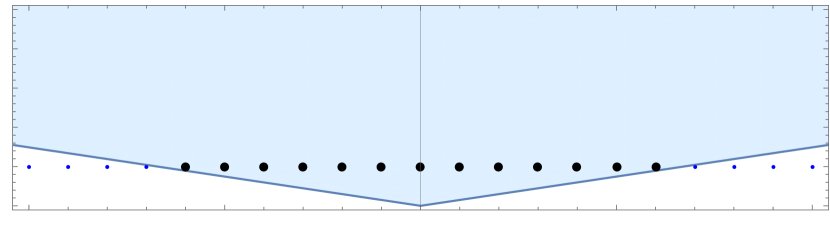
Figure 4. The orbit ${\bf x}_{0}\varpi\Gamma_{\infty,q}$ for $\varpi=e$ inside $B_{T}\subset\mathbb{H}$.

Assume for simplicity that $\bigl{(}\begin{smallmatrix}1&\mathbb{Z}\\ &1\end{smallmatrix}\bigr{)}<\Gamma$; then the isotropy group of $\infty$ in $\Gamma(q)$ is

$$\Gamma_{\infty,q}\ :=\ \bigl{(}\begin{smallmatrix}1&q\mathbb{Z}\\ &1\end{smallmatrix}\bigr{)}\ =\ \Gamma(q)\cap\Gamma_{\infty}.$$

Certainly the orbit $\mathcal{O}_{q,\varpi}$ contains the points

$${\bf x}_{0}\varpi\Gamma_{\infty,q}\ \subset\ \mathcal{O}_{q,\varpi},$$

so

$$\mathcal{N}_{q,\varpi}(T)\ \geq\ |{\bf x}_{0}\varpi\Gamma_{\infty,q}\cap B_{T}|.$$

Converting Figure 3(c) from the disk $\mathbb{D}$ to the hyperbolic plane $\mathbb{H}$, we show in Figure 4 how the shaded region $B_{T}$ contains the orbit points $\varpi\Gamma_{\infty,q}$ for $\varpi=e$. A moment’s reflection (or rather, translation) shows that (1.37) holds for this orbit.

Something similar would happen if one were to take congruence cosets with the subgroups $\Gamma_{0}(q):=\{\bigl{(}\begin{smallmatrix}a&b\\ c&d\end{smallmatrix}\bigr{)}\in\Gamma:c\equiv 0(q)\}$, say, instead of $\Gamma(q)$. The isotropy group $\Gamma_{\infty}$ would now remain unchanged, but the same picture shows that, for the identity coset (with $\varpi=e$), the number of points in an orbit is $\gg T$, whereas is average count should be of order $T/q$. We leave it as an interesting challenge to develop sieve methods which apply to this non-uniformly distributed (in the archimedean ordering) setting.

References

- [BBKT14] Valentin Blomer, Farrell Brumley, Alex Kontorovich, and Nicolas Templier. Bounding hyperbolic and spherical coefficients of Maass forms. J. Théor. Nombres Bordeaux, 26(3):559–579, 2014.
- [Bea83] Alan F. Beardon. The Geometry of Discrete Groups, volume 91 of Graduate Texts in Mathematics. Springer-Verlag, New York, 1983.
- [BGS10] Jean Bourgain, Alex Gamburd, and Peter Sarnak. Affine linear sieve, expanders, and sum-product. Invent. Math., 179(3):559–644, 2010.
- [BGS11] J. Bourgain, A. Gamburd, and P. Sarnak. Generalization of Selberg’s 3/16th theorem and affine sieve. Acta Math, 207:255–290, 2011.
- [BK14] Jean Bourgain and Alex Kontorovich. The affine sieve beyond expansion I: thin hypotenuses, 2014. To appear, IMRN, arXiv:1307.3535.
- [BKS10] J. Bourgain, A. Kontorovich, and P. Sarnak. Sector estimates for hyperbolic isometries. GAFA, 20(5):1175–1200, 2010.
- [Blo08] Valentin Blomer. Sums of Hecke eigenvalues over values of quadratic polynomials. Int. Math. Res. Not. IMRN, (16):Art. ID rnn059. 29, 2008.
- [BR98] Joseph Bernstein and André Reznikov. Sobolev norms of automorphic functionals and Fourier coefficients of cusp forms. C. R. Acad. Sci. Paris Sér. I Math., 327(2):111–116, 1998.
- [CHH88] M. Cowling, U. Haagerup, and R. Howe. Almost matrix coefficients. J. Reine Angew. Math., 387:97–110, 1988.
- [Del42] J. Delsarte. Sur le gitter fuchsien. C. R. Acad. Sci. Paris, 214:147–179, 1942.
- [Del74] Pierre Deligne. La conjecture de Weil. I. Inst. Hautes Études Sci. Publ. Math., (43):273–307, 1974.
- [DG10] A. Diaconu and P. Garrett. Subconvexity bounds for automorphic -functions. J. Inst. Math. Jussieu, 9(1):95–124, 2010.
- [DGG12] Adrian Diaconu, Paul Garrett, and Dorian Goldfeld. Moments for -functions for . In Contributions in analytic and algebraic number theory, volume 9 of Springer Proc. Math., pages 197–227. Springer, New York, 2012.
- [Dol98] Dmitry Dolgopyat. On decay of correlations in Anosov flows. Ann. of Math. (2), 147(2):357–390, 1998.
- [DRS93] W. Duke, Z. Rudnick, and P. Sarnak. Density of integer points on affine homogeneous varieties. Duke Math. J., 71(1):143–179, 1993.
- [EM93] A. Eskin and C. McMullen. Mixing, counting and equidistribution in lie groups. Duke Math. J., 71:143–180, 1993.
- [GGPS66] I. M. Gelfand, M. I. Graev, and I. I. Pjateckii-Shapiro. Teoriya predstavlenii i avtomorfnye funktsii. Generalized functions, No. 6. Izdat. “Nauka”, Moscow, 1966.
- [GJ78] Stephen Gelbart and Hervé Jacquet. A relation between automorphic representations of and . Ann. Sci. École Norm. Sup. (4), 11(4):471–542, 1978.
- [Goo86] A. Good. The convolution method for Dirichlet series. In The Selberg trace formula and related topics (Brunswick, Maine, 1984), volume 53 of Contemp. Math., pages 207–214. Amer. Math. Soc., Providence, RI, 1986.
- [GRS13] Amit Ghosh, Andre Reznikov, and Peter Sarnak. Nodal domains of Maass forms I. Geom. Funct. Anal., 23(5):1515–1568, 2013.
- [HK14] J. Hong and A. Kontorovich. Almost prime coordinates for anisotropic and thin Pythagorean orbits, 2014. To appear, Israel J. Math. arXiv:1401.4701.
- [HKKL13] Thomas A. Hulse, E. Mehmet Kiral, Chan Ieong Kuan, and Li-Mei Lim. Counting square discriminants, 2013. Preprint, arXiv:1307.6606.
- [Hoo63] Christopher Hooley. On the number of divisors of a quadratic polynomial. Acta Math., 110:97–114, 1963.
- [Hub56] H. Huber. über eine neue Klasse automorpher Funktionen und ein Gitterpunktproblem in der hyperbolischen Ebene. i. Comment. Math. Helv., 30:20–62, 1956.
- [IK04] Henryk Iwaniec and Emmanuel Kowalski. Analytic number theory, volume 53 of American Mathematical Society Colloquium Publications. American Mathematical Society, Providence, RI, 2004.
- [Iwa97] Henryk Iwaniec. Topics in classical automorphic forms. American Mathematical Society, Providence, RI, 1997.
- [KO12] A. Kontorovich and H. Oh. Almost prime Pythagorean triples in thin orbits. J. reine angew. Math., 667:89–131, 2012. arXiv:1001.0370.
- [Kon09] A. Kontorovich. The hyperbolic lattice point count in infinite volume with applications to sieves. Duke J. Math., 149(1):1–36, 2009. arXiv:0712.1391.
- [Kon14] Alex Kontorovich. Levels of distribution and the affine sieve. Ann. Fac. Sci. Toulouse Math. (6), 23(5):933–966, 2014.
- [KS03] H. Kim and P. Sarnak. Refined estimates towards the Ramanujan and Selberg conjectures. J. Amer. Math. Soc., 16(1):175–181, 2003.
- [LP82] P.D. Lax and R.S. Phillips. The asymptotic distribution of lattice points in Euclidean and non-Euclidean space. Journal of Functional Analysis, 46:280–350, 1982.
- [LS10] Jianya Liu and Peter Sarnak. Integral points on quadrics in three variables whose coordinates have few prime factors. Israel J. Math, 178:393–426, 2010.
- [Mar04] Grigoriy A. Margulis. On some aspects of the theory of Anosov systems. Springer Monographs in Mathematics. Springer-Verlag, Berlin, 2004. With a survey by Richard Sharp: Periodic orbits of hyperbolic flows, Translated from the Russian by Valentina Vladimirovna Szulikowska.
- [MO13] Amir Mohammadi and Hee Oh. Matrix coefficients, counting and primes for orbits of geometrically finite groups, 2013. To appear, JEMS.
- [MV10] Philippe Michel and Akshay Venkatesh. The subconvexity problem for . Publ. Math. Inst. Hautes Études Sci., (111):171–271, 2010.
- [Nau05] Frédéric Naud. Expanding maps on Cantor sets and analytic continuation of zeta functions. Ann. Sci. École Norm. Sup. (4), 38(1):116–153, 2005.
- [NS10] Amos Nevo and Peter Sarnak. Prime and almost prime integral points on principal homogeneous spaces. Acta Math., 205(2):361–402, 2010.
- [OS13] Hee Oh and Nimish A. Shah. Equidistribution and counting for orbits of geometrically finite hyperbolic groups. J. Amer. Math. Soc., 26(2):511–562, 2013.
- [OS14] Hee Oh and Nimish A. Shah. Limits of translates of divergent geodesics and integral points on one-sheeted hyperboloids. Israel J. Math., 199(2):915–931, 2014.
- [Pat75] S. J. Patterson. The Laplacian operator on a Riemann surface. Compositio Math., 31(1):83–107, 1975.
- [Pat76] S.J. Patterson. The limit set of a Fuchsian group. Acta Mathematica, 136:241–273, 1976.
- [PS01] Yiannis N. Petridis and Peter Sarnak. Quantum unique ergodicity for and estimates for -functions. J. Evol. Equ., 1(3):277–290, 2001. Dedicated to Ralph S. Phillips.
- [Sar81] Peter Sarnak. Asymptotic behavior of periodic orbits of the horocycle flow and Eisenstein series. Comm. Pure Appl. Math., 34(6):719–739, 1981.
- [Sar84] Peter Sarnak. Additive number theory and Maass forms. In Number theory (New York, 1982), volume 1052 of Lecture Notes in Math., pages 286–309. Springer, Berlin, 1984.
- [Sar85] Peter C. Sarnak. Fourth moments of grossencharakteren zeta functions. Comm. Pure and Applied Math., 38:167–178, 1985.
- [Sel56] A. Selberg. Harmonic analysis and discontinuous groups in weakly symmetric Riemannian spaces with applications to Dirichlet series. J. Indian Math. Soc. (N.S.), 20:47–87, 1956.
- [Sha00] Yehuda Shalom. Rigidity, unitary representations of semisimple groups, and fundamental groups of manifolds with rank one transformation group. Ann. of Math. (2), 152(1):113–182, 2000.
- [Str04] A. Strombergsson. On the uniform equidistribution of long closed horocycles. Duke Math. J., 123:507–547, 2004.
- [SU15] Peter Sarnak and Adrián Ubis. The horocycle flow at prime times. J. Math. Pures Appl. (9), 103(2):575–618, 2015.
- [Sul84] D. Sullivan. Entropy, Hausdorff measures old and new, and limit sets of geometrically finite Kleinian groups. Acta Math., 153(3-4):259–277, 1984.
- [Tit51] E. C. Titchmarsh. The Theory of the Riemann Zeta-Function. Oxford Univ. Press, London/New York, Oxford, 1951.
- [TT13] Nicolas Templier and Jacob Tsimerman. Non-split sums of coefficients of -automorphic forms. Israel J. Math., 195(2):677–723, 2013.
- [Ven10] Akshay Venkatesh. Sparse equidistribution problems, period bounds and subconvexity. Ann. of Math. (2), 172(2):989–1094, 2010.
- [Zag81] D. Zagier. Eisenstein series and the Riemann zeta function. In Automorphic forms, representation theory and arithmetic (Bombay, 1979), volume 10 of Tata Inst. Fund. Res. Studies in Math., pages 275–301. Tata Inst. Fundamental Res., Bombay, 1981.