Lightest Kaluza-Klein graviton mode in a backreacted Randall-Sundrum scenario

Abstract

In search of extra dimensions in the ongoing LHC experiments, signatures of Randall-Sundrum (RS) lightest KK graviton have been one of the main focus in recent years. The recent data from the dilepton decay channel at the LHC has determined the experimental lower bound on the mass of the RS lightest Kaluza-Klein (KK) graviton for different choices of underlying parameters of the theory. In this work we explore the effects of the backreaction of the bulk scalar field, which is employed to stabilise the RS model, in modifying the couplings of the lightest KK graviton with the standard model (SM) matter fields located on the visible brane. In such a modified background geometry we show that the coupling of the lightest KK graviton with the SM matter fields gets a significant suppression due to the inclusion of the backreaction of the bulk stabilising scalar field. This implies that the backreaction parameter weakens the signals from RS scenario in collider experiments which in turn explains the non-visibility of KK graviton in colliders. Thus we show that the modulus stabilisation plays a crucial role in the search of warped extra dimensions in collider experiments.

Introduction

Till date, the world of subatomic particles, are best described by the Standard Model (SM) of elementary particles. The validity of the SM has been confirmed with a great accuracy in several experiments upto TeV scale. The recent discovery of Higgs boson in Large Hadron Collider(LHC) indeed is a major success story in this endeavour. Such a successful theory however continues to encounter a longstanding but unresolved question in the context of the stability of the mass of Higgs boson against large radiative correction, known as gauge hierarchy/fine tuning problem. Two most popular models, proposed in the context of this problem, are Supersymmtery and extra-dimensional models [1, 2, 3, 4, 5, 6, 7, 8]. In absence of any signature of supersymmetry near TeV scale so far, the significance of the presence of extra dimension continues to grow. Among these models the warped geometry model proposed by Randall and Sundrum[4] assumed a special significance because a) it resolves the gauge hierarchy problem without introducing any other intermediate scale in the theory, b) the modulus of the extra dimension can be stabilised by introducing a bulk scalar field[9] without any unnatural fine tuning of the parameter of the model.
It may also be mentioned that a warped solution, though not exactly same as RS model, can be found from string theory which as a fundamental theory predicts inevitable existence of extra dimensions [10].

Due to these features, detectors in LHC are designed to explore possible signatures of the warped extra dimensions through various decay channels of RS Kaluza-Klein (KK) graviton. While CMS detector searches the signal of extra dimension through the final states of the decay into leptons and hadrons, ATLAS detector is designed to capture the dileptonic decay of the KK gravitons.

Brief description of RS model

The RS model is characterized by the non-factorisable background metric,

$$ds^{2}=e^{-2k|y|}\eta_{\mu\nu}dx^{\mu}dx^{\nu}-dy^{2}$$ (1)

The extra dimensional coordinate is denoted by $y$ and ranges from $-r_{0}$ to $+r_{0}$ following a $S^{1}/Z_{2}$ orbifolding. Here, $r_{0}$ is the compactification radius of the extra dimension. Two 3-branes are located at the orbifold fixed points $y=(0,r_{0})$. The standard model fields are residing on the visible brane and only gravity can propagate in the bulk. The quantity $k=\sqrt{\frac{-\Lambda}{24M^{3}}}$, which is of the order of 4-dimensional Planck scale $M_{Pl}$. Thus $k$ relates the 5D Planck scale $M$ to the 5D cosmological constant $\Lambda$.
The visible and Planck brane tensions are, $V_{hid}=-V_{vis}=24M^{3}k^{2}$. All the dimensionful parameters described above are related to the reduced 4-dimensional Planck scale ${M}_{Pl}$ as,

$$M_{Pl}^{2}=\frac{M^{3}}{k}(1-e^{-2kr_{0}})$$ (2)

For $kr_{0}\approx 36$, the exponential factor present in the background metric, which is often called warp factor, produces a large suppression so that a mass scale of the order of Planck scale is reduced to TeV scale on the visible brane. A scalar mass say mass of Higgs is given as,

$$m_{H}=m_{0}e^{-kr_{0}}$$ (3)

Here, $m_{H}$ is Higgs mass parameter on the visible brane and $m_{0}$ is the natural scale of the theory above which new physics beyond SM is expected to appear [4].
In RS model, the expressions for the mass of first graviton KK mode $m_{1}$ and the coupling $\lambda$ with the SM matter fields on the TeV brane as [11],

$$m_{1}=x_{1}ke^{-kr_{0}}$$ (4)

where $x_{1}$ can be obtained from $J_{1}(x_{n})=0$ [11], and

$$\lambda=\frac{e^{kr_{0}}}{M_{Pl}}$$ (5)

It has been argued in [11] that the value of $k/M_{Pl}$ should be $0.1$ or less for the validity of classical 5-D solution for the metric in RS model. Keeping this constraint in mind, the ATLAS group in LHC estimated the lower bound on the mass of the lightest KK graviton for different values of $k/M_{Pl}$. The absence of KK graviton in dileptonic decay channels put stringent lower bound on KK graviton masses [12, 13]. According to the most recent experimental data [13] at $8$ TeV centre of mass energy and $20$ ${\rm{fb}}^{-1}$ luminosity, the 95% confidence level lower limit on the RS lightest KK graviton mass is further restricted to 2.68 TeV for $k/M_{PL}=0.1$.
We write eq(4) as,

$$m_{1}=x_{1}\frac{k}{M_{Pl}}M_{Pl}e^{-kr_{0}}$$ (6)

From eq.(6), the mass of the RS lightest KK graviton can be tuned accordingly by increasing the warping parameter $e^{-kr_{0}}$ from $10^{-16}$, so that it goes above the recent experimental lower bound proposed by ATLAS for a fixed parameter $k/M_{Pl}$ which is related to coupling parameter in the original RS scenario.
However from eq.(3), it can be seen that if we increase the warping parameter in order to raise the theoretically calculated graviton mass well above the experimental lower bound then one needs to set the fundamental Planck scale of the theory ($m_{0}$) a few order lower than the 4-D Planck scale ($M_{Pl}$) to obtain Higgs mass of the order of $125$ GeV. Therefore the increment of warp factor with the rise of this experimental lower bound on the mass of the RS lightest KK graviton, implies the inclusion of an intermediate energy scale in between the Planck and TeV scale.
It has been mentioned earlier that the extra dimensional modulus in RS model can be stabilised to a value of the order of inverse Planck length by introducing a massive scalar field in the bulk [9]. In this stabilising mechanism, the effect of the backreaction of the bulk scalar field on the background geometry is neglected. Later such warped geometry model was generalised by incorporating the back reaction of the stabilising scalar field on the background metric [14, 15, 16, 17, 18]. We therefore re-examine the mass of the lightest KK graviton and its coupling to the SM matter fields in such a modified warped geometry model endowed with a back-reacted metric due to the stabilising bulk scalar field. In this work we demonstrate that due to the backreaction of the bulk stabilising scalar field on the background geometry, the effective coupling of the lightest KK graviton with the SM matter fields becomes weaker, which in turn can explain the invisibility of RS lightest KK graviton even if its lower mass bound is as low as few hundred GeV which is much below $2.8$ TeV as predicted by ATLAS.
Thus in this scenario we can explain the invisibility of KK graviton without modifying the value of the warping parameter and $m_{0}$ from their respective values in the original RS model.

We organize our work as follows:
In section(LABEL:Genrs), we describe five dimensional warped geometry model which includes the effect of the backreaction of the bulk stabilising scalar field on the background geometry. Section(2) deals with the KK mass modes of graviton in this modified RS background. In section(3), we discuss the lightest KK graviton interaction with the SM matter fields localised on the visible brane. Sections(4) addresses the phenomenological implications and estimates the lower bound on the lightest graviton mass in the background of this back-reacted warped geometry model. Section(5) ends with some concluding remarks.

1 Backreaction of the stabilising scalar field on the background geometry

We consider the five dimensional action as, [16]

$$S= -M^{3}\int d^{5}x\sqrt{g}R^{(5)}+\int d^{5}x\sqrt{g}(\frac{1}{2}\nabla\phi\nabla\phi-V(\phi))$$ (7)

$$-\int d^{4}x\sqrt{g_{4}}\lambda_{P}(\phi)-\int d^{4}x\sqrt{g_{4}}\lambda_{T}(\phi)$$

where $R^{(5)}$ is the five dimensional Ricci scalar, $\phi$ is the bulk scalar field and $V(\phi)$ is the bulk potential term for the scalar field $\phi$, $g_{4}$ is the induced metric on the brane and $\lambda_{P}$, $\lambda_{T}$ are the potential terms on the Planck and TeV branes respectively due to the bulk scalar field. The scalar field $\phi$ in general is a function of both $x^{\mu}$ and $y$. Here, we consider the background VEV of the field $\phi(x^{\mu},y)\equiv\phi(y)$. The 5-dimensional metric ansatz is [16],

$$ds^{2}=e^{-2A(y)}\eta_{\mu\nu}dx^{\mu}dx^{\nu}-dy^{2}$$ (8)

which preserve 4-D Lorentz invariance. The function $e^{-A(y)}$ is the modified warp factor.
As shown in [16], the 5-D coupled equations for the metric and the scalar field are:

$$4A^{\prime 2}-A^{\prime\prime}=-\frac{2\kappa^{2}}{3}V(\phi)-\frac{\kappa^{2}}{3}\sum_{i}\lambda_{i}(\phi)\delta(y-y_{i})$$ (9)

$$A^{\prime 2}=\frac{\kappa^{2}\phi^{{}^{\prime}2}}{12}-\frac{\kappa^{2}}{6}V(\phi)$$ (10)

$$\phi^{{}^{\prime\prime}}=4A^{\prime}\phi^{{}^{\prime}}+\frac{\partial V(\phi)}{\partial\phi}+\sum_{i}\frac{\partial\lambda_{i}(\phi)}{\partial\phi}\delta(y-y_{i})$$ (11)

where $\kappa$ is the five dimensional Newton’s constant which is related to five dimensional Planck mass $M$ by $\kappa^{2}=1/(2M^{3})$. Here prime and $\partial_{\mu}$ denote the derivatives with respect to $y$ and 4-D space time coordinate i.e.. $x^{\mu}$ respectively.
Following the procedure as illustrated in [15, 16], integrating equations (9),(11) on a small interval [$(y_{i}-\epsilon)$, $(y_{i}+\epsilon)$], one finds the jump conditions,

$$A^{\prime}|_{i}=\frac{\kappa^{2}}{3}\lambda_{i}(\phi)$$ (12)

$$\phi^{{}^{\prime}}|_{i}=\frac{\partial\lambda_{i}(\phi)}{\partial\phi}$$ (13)

As stated in [15], to find the solutions for the above equations of motion we actually need to reduce eq.(9-11) to three decoupled first order differential equations such that two of them are separable. The authors of [15] considered a definite form of the potential as,

$$V(\phi)=\frac{1}{8}\left(\frac{\partial W(\phi)}{\partial\phi}\right)^{2}-\frac{\kappa^{2}}{6}W(\phi)^{2}$$ (14)

for some $W(\phi)$.
It is evident that if we implement the two boundary conditions [equations (15, 16)], it solves both first order differential equations $\phi^{\prime}=\frac{1}{2}\frac{\partial W}{\partial\phi}$, $A^{\prime}=\frac{\kappa^{2}}{6}W(\phi)$ along with the Einstein and scalar field equations of motions in eqs.(9-11).

$$\frac{1}{2}W(\phi)|_{y_{i}-\epsilon}^{y_{i}+\epsilon}=\lambda_{i}(\phi)$$ (15)

$$\frac{1}{2}\frac{\partial W(\phi)}{\partial\phi}|_{y_{i}-\epsilon}^{y_{i}+\epsilon}=\frac{\partial\lambda_{i}}{\partial\phi}(\phi)$$ (16)

At this stage we need to make a choice for $W$ to solve for the back reaction of the bulk scalar field on the metric. It has been shown in [16] that inclusion of the back reaction of the stabilising field generates a TeV order mass term for radion which may have interesting phenomenological consequences.
Considering the form of $W(\phi)$, chosen by the author of [15] and [16],

$$W(\phi)=\frac{6k}{\kappa^{2}}-u\phi^{2}$$ (17)

the brane potential terms become,

$$\lambda(\phi)_{+}=W(\phi_{+})+W^{\prime}(\phi_{+})(\phi-\phi_{+})+\gamma_{+}(\phi-\phi_{+})^{2}$$ (18)

$$\lambda(\phi)_{-}=W(\phi_{-})+W^{\prime}(\phi_{-})(\phi-\phi_{-})+\gamma_{-}(\phi-\phi_{-})^{2}$$ (19)

Here +/- are used to represent Planck/TeV brane. Choosing a definite form of $W(\phi)$, the solution for the stabilising scalar field ($\phi$) and the modified warp factor $A(y)$ can be obtained as [15, 16],

$$\phi(y)=\phi_{P}~{}e^{-uy}$$ (20)

$$A(y)=ky+\frac{\kappa^{2}\phi_{P}^{2}}{12}e^{-2uy}$$ (21)

Here $r_{0}$ is the distance between two 3-branes which can be stabilised by matching the VEV $\phi_{P}$ and $\phi_{T}$ of the stabilising scalar field $\phi$ at $0$ (location of the Planck brane) and $r_{0}$ (location of the TeV brane). This implies $ur_{0}={\rm ln}\left(\phi_{P}/\phi_{T}\right)$. Therefore,

$$e^{-ur_{0}}=\frac{\phi_{T}}{\phi_{P}}$$ (22)

From equation (21), we observe that the warp factor has modified from that in the five dimensional Randall-Sundrum model due to the backreaction of the stabilising scalar field. As expected, in the limit $\kappa^{2}\phi_{P}^{2}$, $\kappa^{2}\phi_{T}^{2}\ll 1$ we retrieve the original 5-D RS model.
All the dimensionful parameters described in this model are related to the reduced 4-dimensional Planck scale $\overline{M}_{Pl}$ as,

$$M_{Pl}^{2}=\frac{M^{3}}{k}\bigg{[}\left\{1-\left(\frac{\phi_{P}}{\phi_{T}}\right)^{-\frac{2k}{u}}\right\}$$ (23)

$$-\frac{l^{2}}{3}\left(1+\frac{u}{k}\right)^{-1}\left\{1-\left(\frac{\phi_{P}}{\phi_{T}}\right)^{-2(1+k/u)}\right\}\bigg{]}$$

where, $l=\frac{\kappa\phi_{P}}{\sqrt{2}}$
It was shown in [16] that the factor $e^{-ur_{0}}$ appears in the final expression for the radion mass which may have significant influence on radion phenomenology.
Question that arises now : does the effect of the back reaction significantly modifies the KK graviton phenomenology also? Can one explain the rise in the value of experimental lower mass bound for the lightest graviton KK mode from the effect of the back reaction of the stabilising field? We try to address this question in the following sections.

2 lightest KK mass mode of Graviton in a back-reacted warped geometry

The effective 4-D theory contains massless as well as massive KK tower of gravitons and all these higher excited states are coupled to the standard model fields, located on the TeV brane. Our objective is to determine the mass of the first excited state of the graviton and its coupling with the SM matter fields in a back-reacted RS geometry due to the stabilising bulk scalar field. In this context we wish to explore a possible explanation for the hitherto non-visibility of the RS lightest KK graviton in the collider experiments. The KK mass modes of graviton and its coupling with the SM matter fields in the background of the original RS model, has been evaluated by the authors of [11]. Here we extend the work by incorporating the back reaction of the bulk stabilising scalar field. The tensor fluctuations $h_{\alpha\beta}$ of the flat metric about its Minkowski value can be expressed through a linear expansion, $\tilde{G}_{\alpha\beta}=e^{-2A(y)}(\eta_{\alpha\beta}+\kappa^{*}h_{\alpha\beta})$, where $\kappa^{*}$ is related to the higher dimensional Newton’s constant. In order to find the graviton KK mass modes we expand the 5-dimensional graviton field in terms of the Kaluza-Klein mode expansion

$$h_{\alpha\beta}(x,y)=\sum^{\infty}_{n=0}h^{(n)}_{\alpha\beta}(x)\frac{\chi^{n}(y)}{\sqrt{r}_{0}}$$ (24)

Where $h^{(n)}_{\alpha\beta}(x)$ are the KK modes of the graviton on the visible 3-brane and $\chi^{n}(\phi)$ are the corresponding internal wave functions for the graviton. Imposing the gauge condition, $\partial^{\alpha}h_{\alpha\beta}=0$ and compactifying the extra dimension, we obtain the effective 4-D theory for graviton as,

$$S_{4}=\int d^{4}x[\eta^{\mu\nu}\partial_{\mu}h_{\alpha\beta}^{(n)}(x)\partial_{\nu}h^{\alpha\beta(n)}(x)-m_{n}^{2}h_{\alpha\beta}^{(n)}(x)h^{\alpha\beta(n)}(x)]$$ (25)

provided,

$$\partial_{y}[e^{-4A(y)}\partial_{y}\chi^{n}(y)]+m_{n}^{2}e^{-2A(y)}\chi^{n}(y)=0$$ (26)

and the orthonormality conditions

$$\frac{1}{r_{0}}\int_{-r_{0}}^{+r_{0}}e^{-2A(y)}\chi^{n_{1}}(y)\chi^{n_{2}}(y)dy=\delta_{n_{1}}\delta_{n_{2}}$$ (27)

are satisfied.

Using $l=\frac{\kappa\phi_{P}}{\sqrt{2}}$ the warp factor can be expressed as,

$$A(y)=ky+\frac{l^{2}}{6}e^{-2uy}$$ (28)

For $l<\sqrt{6}$, we use a leading order approximation for the series expansion of $e^{\frac{l^{2}}{6}e^{-2uy}}$.
For $n=0$ i.e.. zeroth mode of graviton, the differential equation for $\chi^{0}$ turns out to be,

$$\partial_{y}[e^{-4A(y)}\partial_{y}\chi^{0}(y)]=0$$ (29)

Solving the above differential equation and applying the continuity condition for the graviton wavefunction at the two orbifold fixed points we obtain

$$\chi^{0}=c_{1}~{}=~{}{\rm constant}$$ (30)

Normalising the resulting wavefunction from eq.(27), we finally get,

$$\chi^{0}=\sqrt{kr_{0}}\bigg{[}(1-e^{-2kr_{0}})(1-\frac{l^{2}}{3})\bigg{]}^{-1/2}$$ (31)

In order to find the solution for the higher KK graviton modes we define a set of new variables $\chi^{n}(y)=e^{2A(y)}\tilde{\chi}^{n}$ and $z_{n}=\frac{m_{n}}{k}e^{A(y)}=\frac{m_{n}}{k}e^{ky}(1+\frac{l^{2}}{6}e^{-2uy})$. At $y=r_{0}$ the exponential series contains the factor $e^{-ur_{0}}=\frac{\phi_{T}}{\phi_{P}}<1$, for $u>0$.
In terms of these new set of variables we obtain the following differential equation for the graviton higher mode wave function,

$$z_{n}^{2}\frac{d^{2}\tilde{\chi}^{n}}{dz_{n}^{2}}+z_{n}\frac{d\tilde{\chi}^{n}}{dz_{n}}+\left[z_{n}^{2}-4\right]\tilde{\chi}^{n}=0$$ (32)

Solving the above equation we finally arrive at the solution for $\chi^{n}$,

$$\chi^{n}(y)=\frac{e^{2A(y)}}{N_{n}}\bigg{[}J_{2}\left(\frac{m_{n}}{k}e^{A(y)}\right)+\alpha_{n}Y_{2}\left(\frac{m_{n}}{k}e^{A(y)}\right)\bigg{]}$$ (33)

where $N_{n}$ is the normalization constant for the wave function $\chi^{n}$. $J_{2}$, $Y_{2}$ are the Bessel function and Neumann function of order 2 and $\alpha_{n}$ is an arbitrary constant. The KK mass modes of the graviton (i.e.. $m_{n}$) and $\alpha_{n}$ can be found from the continuity condition of the wave function at the two orbifold fixed points i.e.. at $y=r_{0}$ and $y=0$. The continuity condition at $y=0$ implies $\alpha_{n}\ll 1$ as $m_{n}/k\ll 1$. This leads to,

$$\chi^{n}(y)=\frac{e^{2A(y)}}{N_{n}}J_{2}\left(\frac{m_{n}}{k}e^{A(y)}\right)$$ (34)

The continuity condition at $y=r_{0}$, provides

$$J_{1}(x_{n})=0$$ (35)

Where,

$$x_{n}=\frac{m_{n}}{k}e^{A(r_{0})}$$ (36)

All these finally result into the expression for KK mass modes of graviton as,

$$m_{n}=x_{n}ke^{-A(r_{0})}$$ (37)

The normalization constant $N_{n}$ for graviton wave function (34), can now be determined by using the orthonormality condition in equation (27), as

$$N_{n}=\frac{1}{\sqrt{kr_{0}}}e^{A(r_{0})}J_{2}(x_{n})$$ (38)

3 Coupling of the lightest KK graviton with standard model matter fields on the visible brane

Let us consider the interaction of the first excited Kaluza-Klein mode of graviton with the standard model matter fields residing on our universe i.e.. on the visible brane, located at $y=r_{0}$. The solution for tensor fluctuations that appear on our visible brane can be obtained by substituting the solution for $\chi^{n}(y)$ for $n=0$ and higher modes ( see equ.(31), (34) and (38)) in equation (24), at $y=r_{0}$,

$$h_{\alpha\beta}(x,y=r_{0})=\sum^{\infty}_{n=0}h^{(n)}_{\alpha\beta}(x)\frac{\chi^{n}(r_{0})}{\sqrt{r}_{0}}$$

$$= \sqrt{k}\left\{\left(1-\frac{l^{2}}{3}\right)(1-e^{-2kr_{0}})\right\}^{-1/2}h^{0}_{\alpha\beta}(x^{\mu})$$

$$+ \sum^{\infty}_{n=1}\sqrt{k}e^{A(r_{0})}h_{\alpha\beta}^{n}(x^{\mu})$$

The interaction Lagrangian in the effective 4-D theory can be written as,

$$\mathscr{L}|_{int}=-\frac{1}{M^{3/2}}T^{\alpha\beta}(x)h_{\alpha\beta}(x,y=r_{0})$$ (40)

where $T^{\alpha\beta}$ is the energy-momentum tensor of the SM matter fields on the visible brane and we use the relation between the 5-D Planck mass ($M_{5}$) and the 4-D Planck mass ($M_{Pl}$) as shown in eq.(23).
This leads to,

$$\mathscr{L}|_{int}=-\frac{1}{M_{Pl}}T^{\alpha\beta}h_{\alpha\beta}^{0}(x^{\mu})$$

$$- \frac{e^{A(r_{0})}}{M_{Pl}}\bigg{[}\left\{1-\left(\frac{\phi_{P}}{\phi_{T}}\right)^{-\frac{2k}{u}}\right\}-\frac{l^{2}}{3}\left(1+\frac{u}{k}\right)^{-1}$$

$$\left\{1-\left(\frac{\phi_{P}}{\phi_{T}}\right)^{-2(1+k/u)}\right\}\bigg{]}^{1/2}\sum^{\infty}_{n=1}T^{\alpha\beta}h_{\alpha\beta}^{n}(x^{\mu})$$

If we concentrate on the first excited KK mass mode of graviton and its interaction with SM matter fields on the TeV brane, the mass term can be identified as,

$$m_{1}=x_{1}ke^{-A(r_{0})}$$ (42)

while the interaction term of the first excited KK mode of graviton with the SM matter fields on the TeV brane is,

$$\Lambda|_{int}\cong\frac{e^{A(r_{0})}}{M_{Pl}}\bigg{[}\left\{1-\left(\frac{\phi_{P}}{\phi_{T}}\right)^{-\frac{2k}{u}}\right\}-\frac{l^{2}}{3}\left(1+\frac{u}{k}\right)^{-1}$$ (43)

$$\left\{1-\left(\frac{\phi_{P}}{\phi_{T}}\right)^{-2(1+k/u)}\right\}\bigg{]}^{1/2}$$

4 Phenomenological implications

In the previous section we have given a description of the KK mass modes of graviton and the interaction of the first excited KK mode of graviton with the SM matter fields on the visible brane in the context of the back-reacted RS model. In eq.(43), we denote the term

$$\bigg{[}\left\{1-\left(\frac{\phi_{P}}{\phi_{T}}\right)^{-\frac{2k}{u}}\right\}$$ (44)

$$-\frac{l^{2}}{3}\left(1+\frac{u}{k}\right)^{-1}\left\{1-\left(\frac{\phi_{P}}{\phi_{T}}\right)^{-2(1+k/u)}\right\}\bigg{]}^{1/2}=\beta$$

The parameter $\beta$ gives the modification of the coupling of KK graviton with the SM matter fields from that evaluated in the original five dimensional RS model.
In order to address the gauge hierarchy problem we assume that the modified warp factor produces same warping as in the original RS scenario. Therefore,

$$A(0)-A(r_{0})=-37$$ (45)

The above condition produces the following correlation among the parameters $l$, $k/u$ and $\frac{\phi_{P}}{\phi_{T}}$:

$$\frac{k}{u}=\frac{1}{{\rm ln}(\frac{\phi_{P}}{\phi_{T}})}\bigg{[}37+\frac{l^{2}}{6}(1-\frac{\phi_{T}^{2}}{\phi_{P}^{2}})\bigg{]}$$ (46)

The eq.(46) dictates that for a particular choice of $\phi_{P}/\phi_{T}$ and $l$, fixes the value of the parameter $k/u$ the value of $l<\sqrt{6}$ and $\phi_{P}/\phi_{T}>1$. We explore the parameter space by varying the backreaction parameter $l=1.68,1.7,1.71..$, and for each $l$ by varying $\phi_{P}/\phi_{T}=1.5,2.5,3.5..$ one can obtain the corresponding values of $k/u$ from eq.(46). After that we evaluate the parameter $\beta$ from eq.(44), which varies over the values $0.17,0.20,0.22...$ corresponding to our different choices of the parameters of the model.
The values of $\beta$ clearly points out that there is a significant amount of suppression in the dilepton decay channel of the lightest KK graviton over that evaluated in the original RS scenario. This implies that for appropriate choice of the parameters, the effect of back reaction of the bulk stabilising scalar field on the background geometry of a warped extra dimensional model can effectively suppress the coupling parameter of the lightest KK graviton with the SM matter fields. This in turn reduces the value of the lower bound on the the mass of the lightest KK graviton. For example , the lower bound on the mass of the RS lightest KK graviton, say for $\frac{k}{M_{Pl}}=0.1$ now can be substantially lower than $\sim 2.8$ TeV ( lower mass bound without back reaction ) for appropriate choice of the parameter $l$.
Fig.1 clearly brings out the dependence of the lower mass bound of first KK mode of graviton with parameter $l$, for different choices of $k/M_{Pl}$ which indicates a significant suppression from the lower mass bound proposed by ATLAS for the original RS model.
We fix $\phi_{P}/\phi_{T}=1.5$ and write $\beta$ in terms of $l$ by replacing $k/u$ from eq(46). We then plot modified lower mass bound of first excited KK mode of graviton with $l$.

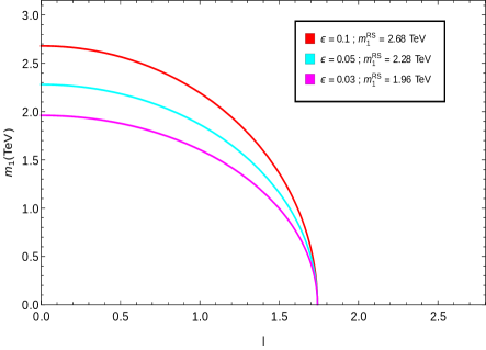
Figure 1: Dependence of the new mass bound of first KK graviton on parameter $l$ for different choices of $k/M_{Pl}$

In summary, the modulus stabilisation mechanism effectively reduces the lower bound of the mass of the lightest KK graviton by a factor $\beta$ which for appropriate choice of the parameter values can be five-ten times lower than that in the original RS scenario.

5 Conclusion

We consider a generalised version of RS model where the effect of the backreaction due to the stabilising bulk scalar field on the background spacetime has been taken into consideration. We aim to study the contribution of this backreaction on the mass of the lightest KK graviton and its couplings to the SM matter fields.
Since the modulus stabilisation in braneworld model is an important requirement to make the prediction of the model more robust, it is therefore worthwhile to look for experimental supports for the model in its stabilised version. Our study strongly suggests that due to the inclusion of the back reaction of the stabilising scalar field, the estimated value of the lower bound of the mass of the lightest KK graviton by the ongoing collider experiments ($m_{1}=\sim 2.8$ TeV for $k/M_{Pl}=0.1$), may get reduced by approximately five-ten times for a fixed $k/M_{Pl}$. In summary, the backreaction of the bulk stabilising scalar field inevitably suppresses the lower bound of the mass of the lightest KK graviton implying that there is no requirement to fine tune any parameter like warp factor or $m_{0}$ (natural scale of the theory) to justify the estimated lower bound on the mass of RS lightest KK graviton from the ongoing collider experiments.

Acknowledgement

We thank Sourov Roy, Shankha Banerjee and Srimoy Bhattacharya for many illuminating discussions.

References

- [1] N. Arkani-Hamed, S. Dimopoulos, G. Dvali, Phys. Lett. B 429 (1998) 263; N. Arkani-Hamed, S. Dimopoulos, G. Dvali, Phys. Rev. D 59 (1999) 086004; I. Antoniadis, N. Arkani-Hamed, S. Dimopoulos, G. Dvali, Phys. Lett. B 436 (1998) 257.
- [2] I. Antoniadis, Phys. Lett. B 246, 377 (1990); J. D. Lykken, Phys. Rev. D 54, 3693 (1996); R. Sundrum, ibid. 59, 085009 (1999); K. R. Dienes, E. Dudas, and T. Gherghetta, Phys. Lett. B 436, 55 (1998); G. Shiu and S. H. Tye, Phys. Rev. D 58, 106007 (1998); Z.Kakushadze and S. H. Tye, Nucl. Phys. B548, 180 (1990).
- [3] P. Horava and E. Witten, Nucl. Phys. B475, 94 (1996); B460, 506 (1996)
- [4] L. Randall and R. Sundrum, Phys. Rev. Lett. 83, 3370 (1999); ibid 83, 4690 (1999).
- [5] L. Randall, R. Sundrum, Phys. Rev. Lett. 83 (1999) 4690
- [6] N. Arkani-Hamed, S. Dimopoulos, G. Dvali, and N. Kaloper, Phys. Rev. Lett. 84, 586 (2000); J. Lykken and L. Randall, J. High Energy Phys. 06, 014 (2000); C. Csa´ki and Y. Shirman, Phys. Rev. D 61, 024008 (2000).
- [7] N. Kaloper, Phys. Rev. D 60, 123506 1999; T. Nihei, Phys. Lett. B 465, 81 (1999); H. B. Kim and H. D. Kim, Phys. Rev. D 61, 064003 (2000).
- [8] A. G. Cohen and D. B. Kaplan, Phys. Lett. B 470, 52 (1999); C. P. Burgess, L. E. Ibanez, and F. Quevedo, ibid. 447, 257 (1999); A. Chodos and E. Poppitz, ibid. 471, 119 (1999); T. Gherghetta and M. Shaposhnikov, Phys. Rev. Lett. 85, 240 (2000).
- [9] W.D. Goldberger and M. B. Wise, Phys.Rev.Lett.83, 4922 (1999).
- [10] M.B. Green, J.H. Schwarz and E. Witten, “Superstring Theory”,Vol.I and Vol.II,Cambridge University Press(1987), String Theory, J. Polchinski, Cambridge University Press(1998)
- [11] H. Davoudiasl, J. L. Hewett, and T. G. Rizzo, Phys.Rev.Lett.84,2080 (2000)
- [12] ATLAS Collaboration, Phys. Lett. B 710 (2012) 538-556;
- [13] ATLAS collaboration, G. Aad et al, Phys. Rev. D.90, 052005 (2014)
- [14] J. M. Cline and H. Firouzjahi, hep-ph/0006037
- [15] O. DeWolfe, D. Z. Freedman, S. S. Gubser and A. Karch, Phys. Rev.D.62, 046008.
- [16] C. Csaki, M.L. Graesser and Graham D. Kribs, Phys. Rev.D.63, 065002.
- [17] A. Dey , D. Maity, S. SenGupta. Phys.Rev. D 75 (2007) 107901
- [18] D. Maity, S. SenGupta, S. Sur. Class.Quant.Grav. 26 (2009) 055003