A weak Local Linearization scheme for stochastic differential equations with multiplicative noise

Abstract

In this paper, a weak Local Linearization scheme for Stochastic Differential Equations (SDEs) with multiplicative noise is introduced. First, for a time discretization, the solution of the SDE is locally approximated by the solution of the piecewise linear SDE that results from the Local Linearization strategy. The weak numerical scheme is then defined as a sequence of random vectors whose first moments coincide with those of the piecewise linear SDE on the time discretization. The rate of convergence is derived and numerical simulations are presented for illustrating the performance of the scheme.

1 Introduction

During 30 years the class of local linearization integrators has been developed for different types of deterministic and random differential equations. The essential principle of such integration methods is the piecewise linearization of the given differential equation to obtain consecutive linear equations that are explicitly solved at each time step. This general approach has worked well for the classes of ordinary, delay, random and stochastic differential equations with additive noise. Key element of such success is the use of explicit solutions or suitable approximations for the resulting linear differential equations. Precisely, the absence of explicit solution or adequate approximation for linear Stochastic Differential Equations (SDEs) with multiplicative noise is the main reason of the limited application of the Local Linearization approach to nonlinear SDEs with multiplicative noise. For these equations, the available local linearization integrators are of two types: the introduced in [2] for scalar equations and the considered in [13, 14, 15]. The former uses the explicit solution of the scalar linear equations with multiplicative noise, while the latter employs the solution of the linear equation with additive noise that locally approximates the nonlinear equation.

Directly related to the development of the local linearization integrators is the concept of Local Linear approximations (see, e.g., [6, 7, 9]). These approximations to the solution of the differential equations are defined as the continuous time solution of the piecewise linear equations associated to the Local Linearization method. These continuous approximations have played a fundamental role for studying the convergence, stability and dynamics of the local linearization integrators for all the classes of differential equations mentioned above with the exception of the SDEs with multiplicative noise. For this last class of equations, the Local Linear approximations have only been used for constructing piecewise approximations to the mean and variance of the states in the framework of continuous-discrete filtering problems (see [9]).

The purpose of this work is to construct a weak Local Linearization integrator for SDEs with multiplicative noise based on suitable weak approximation to the solution of piecewise linear SDEs with multiplicative noise. For this, we cross two ideas: 1) as in [9], the use of the Local Linear approximations for constructing piecewise approximations to the mean and variance of the SDEs with multiplicative noise; and 2) as in [3], at each integration step, the generation of a random vector with the mean and variance of the Local Linear approximation at this integration time. For implementing this, new formulas recently obtained in [5] for the mean and variance of the solution of linear SDEs with multiplicative noise are used, which are computationally more efficient than those formerly proposed in [8, 9]. Notice that this integration approach is conceptually different to that usually employed for designing weak integrators for SDEs. Typically, these integrators are derived from a truncated Ito-Taylor expansion of the equation’s solution at each integration step, and include the generation of random variables with moments equal to those of the involved multiple Ito integrals [10, 11].

The paper is organized as follows. After some basic notations in Section 2, the new Local Linearization integrator is introduced in Section 3. Its rate of convergence is derived in Section 4 and, in the last section, numerical simulations are presented in order to illustrate the performance of the numerical integrator.

2 Basic notations

Let us consider the SDE with multiplicative noise

$$X_{t}=X_{t_{0}}+\int_{t_{0}}^{t}f\left(s,X_{s}\right)ds+\sum_{k=1}^{m}\int_{t_{0}}^{t}g^{k}\left(s,X_{s}\right)dW_{s}^{k},\quad\quad\forall t\in[t_{0},T],$$ (1)

where $f,g^{k}:\left[t_{0},T\right]\times\mathbb{R}^{d}\rightarrow\mathbb{R}^{d}$ are smooth functions, $W^{1},\ldots,W^{m}$ are independent Wiener processes on a filtered complete probability space $\left(\Omega,\mathfrak{F},\left(\mathfrak{F}_{t}\right)_{t\geq t_{0}},\mathbb{P}\right)$, and $X_{t}$ is an adapted $\mathbb{R}^{d}$-valued stochastic process. In addition, let us assume the usual conditions for the existence and uniqueness of a weak solution of (1) with bounded moments (see, e.g., [10]).

Throughout this paper, we consider the time discretization $t_{0}=\tau_{0}<\tau_{1}<\dots<\tau_{N}=T$ with $\tau_{n+1}-\tau_{n}\leq\Delta$ for all $n=0,\ldots,N-1$ and $\Delta>0$. We use the same symbol $K\left(\cdot\right)$ (resp., $K$) for different positive increasing functions (resp., positive real numbers) having the common property to be independent of $\left(\tau_{k}\right)_{k=0,\ldots,N}$. Moreover, $A^{\mathbf{\top}}$ stands for the transpose of the matrix $A$, and $\left|\cdot\right|$ denotes the Euclidean norm for vectors or the Frobenious norm for matrices. By $\mathcal{C}_{P}^{\ell}\left(\mathbb{R}^{d},\mathbb{R}\right)$ we mean the collection of all $\ell$-times continuously differentiable functions $g:\mathbb{R}^{d}\rightarrow\mathbb{R}$ such that $g$ and all its partial derivatives of orders $1,2,\ldots,\ell$ have at most polynomial growth.

3 Numerical method

Suppose that $z_{n}\approx X_{\tau_{n}}$ with $n=0,\ldots,N-1$. Set $g^{0}=f$. Taking the first-order Taylor expansion of $g^{k}$ yields

$$g^{k}\left(t,x\right)\approx g^{k}\left(\tau_{n},z_{n}\right)+\frac{\partial g^{k}}{\partial x}\left(\tau_{n},z_{n}\right)\left(x-z_{n}\right)+\frac{\partial g^{k}}{\partial t}\left(\tau_{n},z_{n}\right)\left(t-\tau_{n}\right)$$

whenever $x\approx z_{n}$ and $t\approx\tau_{n}$. Therefore

$$X_{t}\approx z_{n}+\sum_{k=0}^{m}\int_{\tau_{n}}^{t}\left(B_{n}^{k}X_{s}+b_{n}^{k}\left(s\right)\right)dW_{s}^{k}\quad\quad\forall t\in\left[\tau_{n},\tau_{n+1}\right],$$

with $W_{s}^{0}=s$, $B_{n}^{k}=\dfrac{\partial g^{k}}{\partial x}\left(\tau_{n},z_{n}\right)$ and

$$b_{n}^{k}\left(s\right)=g^{k}\left(\tau_{n},z_{n}\right)-\frac{\partial g^{k}}{\partial x}\left(\tau_{n},z_{n}\right)z_{n}+\frac{\partial g^{k}}{\partial t}\left(\tau_{n},z_{n}\right)\left(s-\tau_{n}\right).$$ (2)

This follows that, for all $t\in\left[\tau_{n},\tau_{n+1}\right]$, $X_{t}$ can be approximated by

$$Y_{t}=z_{n}+\sum_{k=0}^{m}\int_{\tau_{n}}^{t}\left(B_{n}^{k}Y_{s}+b_{n}^{k}\left(s\right)\right)dW_{s}^{k},\hskip 56.9055pt\forall t\in\left[\tau_{n},\tau_{n+1}\right],$$ (3)

which is the first order Local Linear approximation of $X_{t}$ used in [9]. Hence, $\mathbb{E}\phi\left(X_{\tau_{n+1}}\right)\approx\mathbb{E}\phi\left(Y_{\tau_{n+1}}\right)$ for any smooth function $\phi$, and so $X_{\tau_{n+1}}$ might be weakly approximated by a random variable $z_{n+1}$ such that the first moments of $z_{n+1}-z_{n}$ be similar to those of $Y_{\tau_{n+1}}-z_{n}$. This leads us to the following Local Linearization scheme.

Scheme 1.

Let $\eta_{0}^{1},\ldots,\eta_{0}^{m},\cdots,\eta_{N-1}^{1},\ldots,\eta_{N-1}^{m}$ be i.i.d. symmetric random variables having variance $1$ and finite moments of any order. For a given $z_{0}$, we define recursively $\left(z_{n}\right)_{n=0,\ldots,N}$ by

$$z_{n+1}=\mu_{n}\left(\tau_{n+1}\right)+\sqrt{\sigma_{n}\left(\tau_{n+1}\right)-\mu_{n}\left(\tau_{n+1}\right)\mu_{n}^{\intercal}\left(\tau_{n+1}\right)}\,\eta_{n},$$ (4)

where $\eta_{n}=\left(\eta_{n}^{1},\ldots,\eta_{n}^{m}\right)^{\top}$ and $\mu_{n}\left(t\right)$, $\sigma_{n}\left(t\right)$ satisfy the linear differential equations

$$\mu_{n}\left(t\right)=z_{n}+\int_{\tau_{n}}^{t}\left(B_{n}^{0}\,\mu_{n}\left(s\right)+b_{n}^{0}\left(s\right)\right)ds\quad\quad\forall t\in\left[\tau_{n},\tau_{n+1}\right],$$ (5)

$$\sigma_{n}\left(t\right)=z_{n}z_{n}^{\top}+\int_{\tau_{n}}^{t}\mathcal{L}_{n}\left(s,\sigma_{n}\left(s\right)\right)ds\quad\quad\forall t\in\left[\tau_{n},\tau_{n+1}\right].$$ (6)

Here

$$\mathcal{L}_{n}\left(s,\sigma\right) =\sigma\left(B_{n}^{0}\right)^{\top}+B_{n}^{0}\,\sigma^{\intercal}+\mu_{n}\left(s\right)(b_{n}^{0}\left(s\right))^{\top}+b_{n}^{0}\left(s\right)\mu_{n}^{\intercal}\left(s\right)$$

$$\quad+\sum_{k=1}^{m}\left(B_{n}^{k}\,\sigma\left(B_{n}^{k}\right)^{\top}+B_{n}^{k}\,\mu_{n}\left(s\right)(b_{n}^{k}\left(s\right))^{\top}+b_{n}^{k}\left(s\right)\mu_{n}^{\intercal}\left(s\right)\left(B_{n}^{k}\right)^{\top}+b_{n}^{k}\left(s\right)(b_{n}^{k}\left(s\right))^{\top}\right).$$

Remark 3.1.

From (5) it follows that $\mu_{n}\left(\tau_{n+1}\right)$ is the expected valued of $Y_{\tau_{n+1}}$ given $Y_{\tau_{n}}=z_{n}$. Moreover, (6) implies

$$\sigma_{n}\left(\tau_{n+1}\right)=\mathbb{E}\left(Y_{\tau_{n+1}}Y_{\tau_{n+1}}^{\top}\diagup Y_{\tau_{n}}=z_{n}\right).$$

Remark 3.2.

By construction, Scheme 1 preserves the mean-square stability property that the solution of the linear equation $dX_{t}=\sum_{k=0}^{m}(B^{k}X_{t}+b^{k,1}t+b^{k,0})dW_{t}^{k}$ might have. For instance, if the trivial solution of the homogenous equation $dX_{t}=\sum_{k=0}^{m}B^{k}X_{t}dW_{t}^{k}$ is mean-square asymptotically stable, Scheme 1 inherits this property.

Remark 3.3.

A key point in the implementation of Scheme 1 is the evaluation of just one matrix exponential for computing $\mu_{n}\left(\tau_{n+1}\right)$ and $\sigma_{n}\left(\tau_{n+1}\right)$ at each time step. Indeed, from Theorem 2 in [5],

$$\mu_{n}\left(\tau_{n+1}\right)=z_{n}+\mathcal{L}_{2}e^{\mathcal{M}_{n}(\tau_{n+1}-\tau_{n})}u_{n}$$ (7)

and

$$vec(\sigma_{n}\left(\tau_{n+1}\right))=\mathcal{L}_{1}e^{\mathcal{M}_{n}(\tau_{n+1}-\tau_{n})}u_{n},$$ (8)

where the matrices $\mathcal{M}_{n}$, $\mathcal{L}_{1}$, $\mathcal{L}_{2}$ and the vector $u_{n}$ are given by

$$\mathcal{M}_{n}=\left[\begin{array}[]{cccccc}\mathcal{A}&\mathcal{B}_{5}&\mathcal{B}_{4}&\mathcal{B}_{3}&\mathcal{B}_{2}&\mathcal{B}_{1}\\ \mathbf{0}&\mathcal{C}&\mathcal{I}_{d+2}&0&0&0\\ \mathbf{0}&0&\mathcal{C}&0&0&0\\ \mathbf{0}&0&0&0&2&0\\ \mathbf{0}&0&0&0&0&1\\ \mathbf{0}&\mathbf{0}&\mathbf{0}&0&0&0\end{array}\right],\text{ }u_{n}=\left[\begin{array}[]{c}vec(z_{n}z_{n}^{\intercal})\\ 0\\ r\\ 0\\ 0\\ 1\end{array}\right]\in\mathbb{R}^{d^{2}+2d+7},$$

$\mathcal{L}_{2}=\left[\begin{array}[]{ccc}0_{d\times(d^{2}+d+2)}&\mathcal{I}_{d}&0_{d\times 5}\end{array}\right]$ and $\mathcal{L}_{1}=\left[\begin{array}[]{cc}\mathcal{I}_{d^{2}}&0_{d^{2}\times(2d+7)}\end{array}\right]$, with matrices $\mathcal{A}$, $\mathcal{B}_{i}$, $\mathcal{C}$ and $r$ defined by

$$\mathcal{A}=B_{n}^{0}\oplus B_{n}^{0}+\sum\limits_{k=1}^{m}B_{n}^{k}\otimes(B_{n}^{k})^{\intercal},\text{ \ \ \ }\mathcal{C}=\left[\begin{array}[]{ccc}B_{n}^{0}&b_{n}^{0,1}&B_{n}^{0}z_{n}+b_{n}^{0,0}\\ 0&0&1\\ 0&0&0\end{array}\right],\text{\ \ \ \ \ }r=\left[\begin{array}[]{c}\mathbf{0}_{(d+1)\times 1}\\ 1\end{array}\right],$$

$\mathcal{B}_{1}=vec(\beta_{1})+\beta_{4}z_{n}$, $\mathcal{B}_{2}=vec(\beta_{2})+\beta_{5}z_{n}$, $\mathcal{B}_{3}=vec(\beta_{3})$, $\mathcal{B}_{4}=\beta_{4}\mathcal{L}$, and $\mathcal{B}_{5}=\beta_{5}\mathcal{L}$. Here $\mathcal{L}=\left[\begin{array}[]{ll}\mathcal{I}_{d}&0_{d\times 2}\end{array}\right]$ and

$$\beta_{1}=\sum\limits_{k=1}^{m}b_{n}^{k,0}(b_{n}^{k,0})^{\intercal},\text{ \ \ \ \ }\beta_{2}=\sum\limits_{k=1}^{m}b_{n}^{k,0}(b_{n}^{k,1})^{\intercal}+b_{n}^{k,1}(b_{n}^{k,0})^{\intercal},\text{ \ \ \ \ \ }\beta_{3}=\sum\limits_{k=1}^{m}b_{n}^{k,1}(b_{n}^{k,1})^{\intercal},\text{ }$$

$$\text{\ \ \ }\beta_{4}=b_{n}^{0,0}\oplus b_{n}^{0,0}+\sum\limits_{k=1}^{m}b_{n}^{k,0}\otimes B_{n}^{k}+B_{n}^{k}\otimes b_{n}^{k,0},\text{ \ \ }\beta_{5}=b_{n}^{0,1}\oplus b_{n}^{0,1}+\sum\limits_{k=1}^{m}b_{n}^{k,1}\otimes B_{n}^{k}+B_{n}^{k}\otimes b_{n}^{k,1},$$

being $b_{n}^{k,0}$ and $b_{n}^{k,1}$ defined via (2) as $b_{n}^{k,0}+b_{n}^{k,1}\left(s-\tau_{n}\right)=b_{n}^{k}\left(s\right)$. The symbols $vec$, $\oplus$ and $\otimes$ denote the vectorization operator, the Kronecker sum and the Kronecker product, respectively. $\mathcal{I}_{d}$ is the $d-$dimensional identity matrix. The matrix exponential in (7) and (8) can be efficiently computed via the Padé method with scaling and squaring strategy or via the Krylov subspace method in the case of large system of SDEs (see, e.g., [12]). For autonomous equations or for equations with additive noise, the exponential matrix in (7) and (8) reduces to simpler forms [5].

Remark 3.4.

For SDEs with additive noise, Scheme 1 reduces to the weak order-$1$ Local Linearization scheme introduced in [3].

4 Rate of convergence

Next theorem establishes the linear rate of weak convergence of Scheme 1 when the drift and diffusion coefficients are smooth enough.

Hypothesis 1.

For any $k=0,\ldots,m$ we have $g^{k}\in\mathcal{C}_{P}^{4}\left(\left[t_{0},T\right]\times\mathbb{R}^{d},\mathbb{R}^{d}\right)$. Moreover,

$$\left|g^{k}\left(t,x\right)\right|\leq K\left(1+\left|x\right|\right)\qquad\mbox{ and }\qquad\left|\dfrac{\partial g^{k}}{\partial t}\left(t,x\right)\right|+\left|\dfrac{\partial g^{k}}{\partial x}\left(t,x\right)\right|\leq K$$ (9)

for all $t\in\left[t_{0},T\right]$ and $x\in\mathbb{R}^{d}$.

Theorem 4.1.

In addition to Hypothesis 1, suppose that $X_{t_{0}}$ has finite moments of any order and that for all $\phi\in\mathcal{C}_{P}^{4}\left(\mathbb{R}^{d},\mathbb{R}\right)$,

$$\left|\mathbb{E}\phi\left(X_{t_{0}}\right)-\mathbb{E}\phi\left(z_{0}\right)\right|\leq K\Delta.$$

Then, for all $\phi\in\mathcal{C}_{P}^{4}\left(\mathbb{R}^{d},\mathbb{R}\right)$,

$$\left|\mathbb{E}\phi\left(X_{T}\right)-\mathbb{E}\phi\left(z_{N}\right)\right|\leq K\left(T\right)\Delta,$$

where $z_{N}$ is given by Scheme 1.

Theorem 4.1 is a straightforward result of Theorem 14.5.2 in [10] and the two following Lemmata.

Lemma 4.1.

Under the assumptions of Theorem 4.1, for any $q\geq 1$ we have

$$\mathbb{E}\left(\max_{n=0,\ldots,N}\left|z_{n}\right|^{2q}\right)\leq K\left(T\right)\left(1+\mathbb{E}\left(\left|z_{0}\right|^{2q}\right)\right)$$ (10)

and

$$\mathbb{E}\left(\left|z_{n+1}-z_{n}\right|^{2q}\diagup\mathfrak{F}_{\tau_{n}}\right)\leq K\left(T\right)\left(\tau_{k+1}-\tau_{k}\right)^{q}\left(1+\left|z_{n}\right|^{2q}\right)$$ (11)

for all $n=0,\ldots,N-1$.

Proof.

From Hypothesis 1 it follows that $\left|B_{n}^{k}\right|\leq K$ and

$$\left|b_{n}^{k}\left(s\right)\right|\leq K\left(T\right)\left(1+\left|z_{n}\right|\right)$$ (12)

for all $n=0,\ldots,N-1$, $k=0,\ldots,m$ and $s\in\left[\tau_{n},\tau_{n+1}\right]$. Then, combining Gronwall’s lemma with (5) gives

$$\left|\mu_{n}\left(s\right)\right|\leq K\left(T\right)\left(1+\left|z_{n}\right|\right)\quad\quad\quad\forall s\in\left[\tau_{n},\tau_{n+1}\right].$$ (13)

Since $\left|x\,y^{\top}\right|=\left|x\right|\left|y\right|$ for any $x,y\in\mathbb{R}^{d}$, (12) and (13) lead to

$$\left|\mathcal{L}_{n}\left(s,\sigma\right)\right|\leq K\left|\sigma\right|+K\left(T\right)\left(1+\left|z_{n}\right|^{2}\right)\quad\quad\quad\forall s\in\left[\tau_{n},\tau_{n+1}\right],$$ (14)

where $n=0,\ldots,N-1$ and $\mathcal{L}_{n}$ is as in (6). Using Gronwall’s lemma, (6) and (14) we deduce that

$$\left|\sigma_{n}\left(s\right)\right|\leq K\left(T\right)\left(1+\left|z_{n}\right|^{2}\right)\quad\quad\quad\forall s\in\left[\tau_{n},\tau_{n+1}\right].$$ (15)

Decomposing

$$\widetilde{\sigma}_{n}\left(t\right):=\sigma_{n}\left(t\right)-\mu_{n}\left(t\right)\mu_{n}^{\intercal}\left(t\right)$$

as $\sigma_{n}\left(t\right)-z_{n}z_{n}^{\top}-z_{n}\left(\mu_{n}\left(t\right)-z_{n}\right)^{\top}-\left(\mu_{n}\left(t\right)-z_{n}\right)z_{n}^{\top}-\left(\mu_{n}\left(t\right)-z_{n}\right)\left(\mu_{n}\left(t\right)-z_{n}\right)^{\top}$ we have

$$\widetilde{\sigma}_{n}\left(t\right) =\int_{\tau_{n}}^{t}\mathcal{L}_{n}\left(s,\sigma_{n}\left(s\right)\right)ds-z_{n}\left(\int_{\tau_{n}}^{t}\left(B^{0}_{n}\,\mu_{n}\left(s\right)+b^{0}_{n}\left(s\right)\right)ds\right)^{\top}\quad-\int_{\tau_{n}}^{t}\left(B^{0}_{n}\,\mu_{n}\left(s\right)+b^{0}_{n}\left(s\right)\right)ds\,z_{n}^{\top}$$

$$\quad-\int_{\tau_{n}}^{t}\left(B^{0}_{n}\,\mu_{n}\left(s\right)+b^{0}_{n}\left(s\right)\right)ds\left(\int_{\tau_{n}}^{t}\left(B^{0}_{n}\,\mu_{n}\left(s\right)+b^{0}_{n}\left(s\right)\right)ds\right)^{\top},$$

and so (13), (14) and (15) yields

$$\left|\widetilde{\sigma}_{n}\left(t\right)\right|\leq K\left(T\right)\left(1+\left|z_{n}\right|^{2}\right)\left(t-\tau_{n}\right)\quad\quad\quad\forall t\in\left[\tau_{n},\tau_{n+1}\right].$$ (16)

Iterating (4) we obtain

$$z_{n+1}=z_{0}+\int_{t_{0}}^{\tau_{n+1}}\left(B_{n\left(s\right)}^{0}\,\mu_{n\left(s\right)}\left(s\right)+b_{n\left(s\right)}^{0}\left(s\right)\right)ds+S_{n+1},$$ (17)

where $n=0,\ldots,N-1$, $n\left(t\right)=\max\left\{n=0,\ldots,N:\tau_{n}\leq t\right\}$ and

$$S_{n+1}=\sum_{k=0}^{n}\sqrt{\sigma_{k}\left(\tau_{k+1}\right)-\mu_{k}\left(\tau_{k+1}\right)\mu_{k}^{\intercal}\left(\tau_{k+1}\right)}\,\eta_{k}.$$

Applying Hölder’s inequality we get

$$\left|\int_{t_{0}}^{\tau_{n+1}}\left(B_{n\left(s\right)}^{0}\,\mu_{n\left(s\right)}\left(s\right)+b_{n\left(s\right)}^{0}\left(s\right)\right)ds\right|^{2q}$$

$$\leq\left(\tau_{n+1}-t_{0}\right)^{2q-1}\int_{t_{0}}^{\tau_{n+1}}\left|\left(B_{n\left(s\right)}^{0}\,\mu_{n\left(s\right)}\left(s\right)+b_{n\left(s\right)}^{0}\left(s\right)\right)\right|^{2q}ds,$$

and so (12) and (13) yield

$$\left|\int_{t_{0}}^{\tau_{n+1}}\left(B_{n\left(s\right)}^{0}\,\mu_{n\left(s\right)}\left(s\right)+b_{n\left(s\right)}^{0}\left(s\right)\right)ds\right|^{2q}\leq K\left(T\right)\left(1+\int_{t_{0}}^{\tau_{n+1}}\left|z_{n\left(s\right)}\right|^{2q}ds\right).$$ (18)

Set $S_{0}=0$. For any $n=0,\ldots,N-1$,

$$\mathbb{E}\left(\left|S_{n+1}\right|^{2}\right) =\mathbb{E(}S_{n+1}^{\intercal}S_{n+1})$$

$$=\sum_{k=0}^{n}\mathbb{E}\left(\eta_{k}^{\intercal}\left(\sigma_{k}\left(\tau_{k+1}\right)-\mu_{k}\left(\tau_{k+1}\right)\mu_{k}^{\intercal}\left(\tau_{k+1}\right)\right)\eta_{k}\right)$$

$$=\sum_{k=0}^{n}\sum_{\ell=1}^{d}\mathbb{E}\left(\sigma_{k}\left(\tau_{k+1}\right)^{\ell,\ell}+\left(\mu_{k}\left(\tau_{k+1}\right)^{\ell}\right)^{2}\right).$$

Since $\sigma_{k}\left(\tau_{k+1}\right)=\mathbb{E}\left(Y_{\tau_{k+1}}Y_{\tau_{k+1}}^{\top}\diagup\mathfrak{F}_{\tau_{k}}\right)$, (13) yields

$$\mathbb{E}\left(\left|S_{n+1}\right|^{2}\right)\leq\sum_{k=0}^{n}\left(\mathbb{E}\left(\left|Y_{\tau_{k+1}}\right|^{2}\right)+\mathbb{E}\left|\mu_{k}\left(\tau_{k+1}\right)\right|^{2}\right)<+\infty,$$

and so $\left(S_{n}\right)_{n=0,\ldots,N}$ is a $\left(\mathfrak{F}_{\tau_{n}}\right)_{n=0,\ldots,N}$-square integrable martingale. According to the Burkholder-Davis-Gundy inequality we have

$$\mathbb{E}\left(\max_{k=0,\ldots,n}\left(S_{k}^{j}\right)^{2q}\right)\leq C_{q}\mathbb{E}\left(\left[S^{j},S^{j}\right]_{n}^{q}\right)=C_{q}\mathbb{E}\left(\sum_{k=0}^{n}\left(\left(\sqrt{\widetilde{\sigma}_{k}\left(\tau_{k+1}\right)}\,\eta_{k}\right)^{j}\right)^{2}\right)^{q},$$

where $C_{q}>0$ and $y^{j}$ stands for the $j$-th coordinate of the vector $y$. Applying Hölder’s inequality yields

$$\left(\sum_{k=0}^{n}\left(\tau_{k+1}-\tau_{k}\right)^{1/p}\left(\tau_{k+1}-\tau_{k}\right)^{1/q}\left(\left(\sqrt{\widetilde{\sigma}_{k}\left(\tau_{k+1}\right)}\,\eta_{k}\right)^{j}\right)^{2}/\left(\tau_{k+1}-\tau_{k}\right)\right)^{q}$$

$$\leq\left(\sum_{k=0}^{n}\left(\tau_{k+1}-\tau_{k}\right)\right)^{q-1}\sum_{k=0}^{n}\left(\tau_{k+1}-\tau_{k}\right)\left(\left(\sqrt{\widetilde{\sigma}_{k}\left(\tau_{k+1}\right)}\,\eta_{k}\right)^{j}\right)^{2q}/\left(\tau_{k+1}-\tau_{k}\right)^{q}$$

with $1/p+1/q=1$. Using $\left|\sqrt{\widetilde{\sigma}_{k}\left(\tau_{k+1}\right)}\right|^{2}=\left|\widetilde{\sigma}_{k}\left(\tau_{k+1}\right)\right|$ we obtain

$$\mathbb{E}\left(\max_{k=0,\ldots,n}\left|S_{k}\right|^{2q}\right) \leq\left(Td\right)^{q-1}C_{q}\sum_{k=0}^{n}\mathbb{E}\left(\left(\tau_{k+1}-\tau_{k}\right)\frac{\left|\sqrt{\widetilde{\sigma}_{k}\left(\tau_{k+1}\right)}\right|^{2q}}{\left(\tau_{k+1}-\tau_{k}\right)^{q}}\left|\eta_{k}\right|^{2q}\right)$$

$$\leq\left(Td\right)^{q-1}C_{q}\sum_{k=0}^{n}\mathbb{E}\left(\left(\tau_{k+1}-\tau_{k}\right)\left(\frac{\left|\widetilde{\sigma}_{k}\left(\tau_{k+1}\right)\right|}{\tau_{k+1}-\tau_{k}}\right)^{q}\left|\eta_{k}\right|^{2q}\right).$$

Hence (16) yields

$$\mathbb{E}\left(\max_{k=0,\ldots,n}\left|S_{k}\right|^{2q}\right)\leq K\left(T\right)\mathbb{E}\left(\left|\eta_{0}\right|^{2q}\right)\left(1+\sum_{k=0}^{n}\left(\tau_{k+1}-\tau_{k}\right)\mathbb{E(}\left|z_{k}\right|^{2q})\right).$$ (19)

Using (17), (18) and (19), together with Hölder’s inequality, we get

$$\mathbb{E}\left(\max_{j=0,\ldots,n+1}\left|z_{j}\right|^{2q}\right)\leq K\left(T\right)\left(\mathbb{E}\left|z_{0}\right|^{2q}+1+\sum_{k=0}^{n}\left(\tau_{k+1}-\tau_{k}\right)\mathbb{E(}\left|z_{k}\right|^{2q})\right).$$

The discrete time Gronwall-Bellman lemma now leads to (10).

We proceed to show (11). Using Hölder’s inequality and (13) we obtain

$$\left|\int_{\tau_{n}}^{\tau_{n+1}}\left(B_{n}^{0}\,\mu_{n}\left(s\right)+b_{n}^{0}\left(s\right)\right)ds\right|^{2q} \leq \left(\tau_{n+1}-\tau_{n}\right)^{2q-1}\int_{\tau_{n}}^{\tau_{n+1}}\left(\left|B_{n}^{0}\right|\left|\mu_{n}\left(s\right)\right|+\left|b_{n}^{0}\left(s\right)\right|\right)^{2q}ds$$

$$\leq K\left(T\right)\left(\tau_{n+1}-\tau_{n}\right)^{2q}\left(1+\left|z_{n}\right|^{2q}\right).$$

By (16),

$$\left|\sqrt{\widetilde{\sigma}_{n}\left(\tau_{n+1}\right)}\,\eta_{n}\right|^{2q} \leq\left|\sqrt{\widetilde{\sigma}_{n}\left(\tau_{n+1}\right)}\right|^{2q}\left|\eta_{n}\right|^{2q}$$

$$=\left|\widetilde{\sigma}_{n}\left(\tau_{n+1}\right)\right|^{q}\left|\eta_{n}\right|^{2q}$$

$$\leq K\left(T\right)\left(1+\left|z_{n}\right|^{2q}\right)\left(\tau_{n+1}-\tau_{n}\right)^{q}\left|\eta_{n}\right|^{2q}.$$

Hence

$$\mathbb{E}\left(\left|\sqrt{\widetilde{\sigma}_{n}\left(\tau_{n+1}\right)}\,\eta_{n}\right|^{2q}\diagup\mathfrak{F}_{\tau_{n}}\right)\leq K\left(T\right)\left(1+\left|z_{n}\right|^{2q}\right)\left(\tau_{n+1}-\tau_{n}\right)^{q}\mathbb{E}\left(\left|\eta_{n}\right|^{2q}\right).$$

This implies (11), because

$$\mathbb{E}\left(\left|z_{n+1}-z_{n}\right|^{2q}\diagup\mathfrak{F}_{\tau_{n}}\right) \leq 2^{2q-1}\mathbb{E}\left(\left|\int_{\tau_{n}}^{\tau_{n+1}}\left(B_{n}^{0}\,\mu_{n}\left(s\right)+b_{n}^{0}\left(s\right)\right)ds\right|^{2q}\diagup\mathfrak{F}_{\tau_{k}}\right)$$

$$\quad+2^{2q-1}\mathbb{E}\left(\left|\sqrt{\widetilde{\sigma}_{n}\left(\tau_{n+1}\right)}\,\eta_{n}\right|^{2q}\diagup\mathfrak{F}_{\tau_{n}}\right).$$

∎

Lemma 4.2.

Assume the hypothesis of Theorem 4.1. Let

$$\chi_{n+1}=f\left(\tau_{n},z_{n}\right)\left(\tau_{n+1}-\tau_{n}\right)+\sum_{k=1}^{m}g^{k}\left(\tau_{n},z_{n}\right)\left(W_{\tau_{n+1}}^{k}-W_{\tau_{k}}^{k}\right).$$

Then, for all $n=0,\ldots,N-1$, it is obtained that

$$\left|\mathbb{E}\left(\left(z_{n+1}-z_{n}\right)\diagup\mathfrak{F}_{\tau_{n}}\right)-\mathbb{E}\left(\chi_{n+1}\diagup\mathfrak{F}_{\tau_{n}}\right)\right|\leq K\left(T\right)\left(\tau_{n+1}-\tau_{n}\right)^{2}\left(1+\left|z_{n}\right|\right),$$ (20)

$$\left|\mathbb{E}\left(\left(z_{n+1}-z_{n}\right)\left(z_{n+1}-z_{n}\right)^{\top}\diagup\mathfrak{F}_{\tau_{n}}\right)-\mathbb{E}\left(\chi_{n+1}\chi_{n+1}^{\top}\diagup\mathfrak{F}_{\tau_{n}}\right)\right|\leq K\left(T\right)\left(\tau_{n+1}-\tau_{n}\right)^{2}\left(1+\left|z_{n}\right|^{2}\right),$$ (21)

and

$$\begin{array}[]{c}\left|\mathbb{E}\left(\left(z_{n+1}-z_{n}\right)^{\ell}\left(z_{n+1}-z_{n}\right)\left(z_{n+1}-z_{n}\right)^{\top}\diagup\mathfrak{F}_{\tau_{n}}\right)-\mathbb{E}\left(\chi_{n+1}^{\ell}\chi_{n+1}\chi_{n+1}^{\top}\diagup\mathfrak{F}_{\tau_{n}}\right)\right|\\ \leq K\left(T\right)\left(\tau_{n+1}-\tau_{n}\right)^{2}\left(1+\left|z_{n}\right|^{2}\right).\end{array}$$ (22)

Proof.

Since $B_{n}^{0}\,z_{n}+b_{n}^{0}\left(\tau_{n}\right)=f\left(\tau_{n},z_{n}\right)$,

$$\mu_{n}\left(\tau_{n+1}\right)-z_{n}-f\left(\tau_{n},z_{n}\right)\left(\tau_{n+1}-\tau_{n}\right) = \int_{\tau_{n}}^{\tau_{n+1}}\left(B_{n}^{0}\,\mu_{n}\left(s\right)+b_{n}^{0}\left(s\right)-f\left(\tau_{n},z_{n}\right)\right)ds$$

$$= \int_{\tau_{n}}^{\tau_{n+1}}\left(B_{n}^{0}\left(\mu_{n}\left(s\right)-z_{n}\right)+b_{n}^{0}\left(s\right)-b_{n}^{0}\left(\tau_{n}\right)\right)ds.$$

Using (9) and (13) we deduce that

$$\left|\mu_{n}\left(\tau_{n+1}\right)-z_{n}-f\left(\tau_{n},z_{n}\right)\left(\tau_{n+1}-\tau_{n}\right)\right| \leq K\int_{\tau_{n}}^{\tau_{n+1}}\left(\left|\mu_{n}\left(s\right)-z_{n}\right|+s-\tau_{n}\right)ds$$ (23)

$$\leq K\int_{\tau_{n}}^{\tau_{n+1}}\int_{\tau_{n}}^{s}\left|B_{n}^{0}\,\mu_{n}\left(r\right)+b_{n}^{0}\left(s\right)\right|drds+K\left(\tau_{n+1}-\tau_{n}\right)^{2}$$

$$\leq K\left(T\right)\left(\tau_{n+1}-\tau_{n}\right)^{2}\left(1+\left|z_{n}\right|\right).$$

Since

$$\left|\mathbb{E}\left(\left(z_{n+1}-z_{n}\right)\diagup\mathfrak{F}_{\tau_{n}}\right)-\mathbb{E}\left(\chi_{n+1}\diagup\mathfrak{F}_{\tau_{n}}\right)\right|=\left|\mu_{n}\left(\tau_{n+1}\right)-z_{n}-f\left(\tau_{n},z_{n}\right)\left(\tau_{n+1}-\tau_{n}\right)\right|,$$

(23) yields (20).

From

$$\mathbb{E}\left(\chi_{n+1}\chi_{n+1}^{\top}\diagup\mathfrak{F}_{\tau_{n}}\right)=f\left(\tau_{n},z_{n}\right)f\left(\tau_{n},z_{n}\right)^{\top}\left(\tau_{n+1}-\tau_{n}\right)^{2}+\sum_{k=1}^{m}g^{k}\left(\tau_{n},z_{n}\right)g^{k}\left(\tau_{n},z_{n}\right)^{\top}\left(\tau_{n+1}-\tau_{n}\right)$$

we obtain

$$\left|\mathbb{E}\left(\chi_{n+1}\chi_{n+1}^{\top}\diagup\mathfrak{F}_{\tau_{n}}\right)-\sum_{k=1}^{m}g^{k}\left(\tau_{n},z_{n}\right)(g^{k}\left(\tau_{n},z_{n}\right))^{\top}\left(\tau_{n+1}-\tau_{n}\right)\right|\leq K\left(T\right)\left(\tau_{n+1}-\tau_{n}\right)^{2}\left(1+\left|z_{n}\right|^{2}\right).$$ (24)

As in the proof of Lemma 4.1, we define $\widetilde{\sigma}_{n}\left(t\right):=\sigma_{n}\left(t\right)-\mu_{n}\left(t\right)\mu_{n}\left(t\right)^{\top}$ for any $t\in\left[\tau_{n},\tau_{n+1}\right]$. Then

$$\mathbb{E}\left(\left(z_{n+1}-z_{n}\right)\left(z_{n+1}-z_{n}\right)^{\top}\diagup\mathfrak{F}_{\tau_{n}}\right) =\left(\mu_{n}\left(\tau_{n+1}\right)-z_{n}\right)\left(\mu_{n}\left(\tau_{n+1}\right)-z_{n}\right)^{\top}+\widetilde{\sigma}_{n}\left(\tau_{n+1}\right).$$

Since

$$\widetilde{\sigma}_{n}\left(\tau_{n+1}\right) =\sigma_{n}\left(\tau_{n+1}\right)-z_{n}z_{n}^{\top}-z_{n}\left(\mu_{n}\left(\tau_{n+1}\right)-z_{n}\right)^{\top}-\left(\mu_{n}\left(\tau_{n+1}\right)-z_{n}\right)z_{n}^{\top}$$

$$\quad-\left(\mu_{n}\left(\tau_{n+1}\right)-z_{n}\right)\left(\mu_{n}\left(\tau_{n+1}\right)-z_{n}\right)^{\top},$$

applying (23) yields

$$\left|\mathbb{E}\left(\left(z_{n+1}-z_{n}\right)\left(z_{n+1}-z_{n}\right)^{\top}\diagup\mathfrak{F}_{\tau_{n}}\right)-\sigma_{n}\left(\tau_{n+1}\right)+z_{n}z_{n}^{\top}\right.$$

$$\hskip 85.35826pt\left.+z_{n}f\left(\tau_{n},z_{n}\right)^{\top}\left(\tau_{n+1}-\tau_{n}\right)+f\left(\tau_{n},z_{n}\right)z_{n}^{\top}\left(\tau_{n+1}-\tau_{n}\right)\right|$$

$$\leq K\left(T\right)\left(\tau_{n+1}-\tau_{n}\right)^{2}\left(1+\left|z_{n}\right|^{2}\right).$$

Using (12), (13) and (14), together with Hypothesis 1, we deduce that

$$\left|\mathcal{L}_{n}\left(s,\sigma_{n}\left(s\right)\right)-\mathcal{L}_{n}\left(\tau_{n},z_{n}z_{n}^{\top}\right)\right|\leq K\left(T\right)\left(s-\tau_{n}\right)\left(1+\left|z_{n}\right|^{2}\right),$$

and so

$$\left|\sigma_{n}\left(\tau_{n+1}\right)-z_{n}z_{n}^{\top}-\mathcal{L}_{n}\left(\tau_{n},z_{n}z_{n}^{\top}\right)\left(\tau_{n+1}-\tau_{n}\right)\right| \leq \int_{\tau_{n}}^{\tau_{n+1}}\left|\mathcal{L}_{n}\left(s,\sigma_{n}\left(s\right)\right)-\mathcal{L}_{n}\left(\tau_{n},z_{n}z_{n}^{\top}\right)\right|ds$$

$$\leq K\left(T\right)\left(\tau_{n+1}-\tau_{n}\right)^{2}\left(1+\left|z_{n}\right|^{2}\right).$$

Therefore

$$\left|\mathbb{E}\left(\left(z_{n+1}-z_{n}\right)\left(z_{n+1}-z_{n}\right)^{\top}\diagup\mathfrak{F}_{\tau_{n}}\right)-\sum_{k=1}^{m}g^{k}\left(\tau_{n},z_{n}\right)(g^{k}\left(\tau_{n},z_{n}\right))^{\top}\left(\tau_{n+1}-\tau_{n}\right)\right|$$ (25)

$$\leq K\left(T\right)\left(\tau_{n+1}-\tau_{n}\right)^{2}\left(1+\left|z_{n}\right|^{2}\right),$$

because

$$\mathcal{L}_{n}\left(\tau_{n},z_{n}z_{n}^{\top}\right)=z_{n}f\left(\tau_{n},z_{n}\right)^{\top}+f\left(\tau_{n},z_{n}\right)z_{n}^{\top}+\sum_{k=1}^{m}g^{k}\left(\tau_{n},z_{n}\right)g^{k}\left(\tau_{n},z_{n}\right)^{\top}.$$

Combining (24) with (25) we get (21).

A careful computation shows

$$\mathbb{E}\left(\chi_{n+1}^{\ell}\chi_{n+1}\chi_{n+1}^{\top}\diagup\mathfrak{F}_{\tau_{n}}\right) = f\left(\tau_{n},z_{n}\right)^{\ell}f\left(\tau_{n},z_{n}\right)f\left(\tau_{n},z_{n}\right)^{\top}\left(\tau_{n+1}-\tau_{n}\right)^{3}+f\left(\tau_{n},z_{n}\right)^{\ell}G_{n}G_{n}^{\top}\left(\tau_{n+1}-\tau_{n}\right)^{2}$$

$$+f\left(\tau_{n},z_{n}\right)\left(G_{n}G_{n}^{\top}\right)^{\ell,\cdot}\left(\tau_{n+1}-\tau_{n}\right)^{2}+\left(G_{n}G_{n}^{\top}\right)^{\cdot,\ell}f\left(\tau_{n},z_{n}\right)^{\top}\left(\tau_{n+1}-\tau_{n}\right)^{2},$$

where $G_{n}$ is the $\mathbb{R}^{d\times m}$-matrix whose $\left(i,j\right)$-th element is the $i$-th entry of $g^{j}\left(\tau_{n},z_{n}\right)$. Similarly,

$$\mathbb{E}\left(\left(z_{n+1}-z_{n}\right)^{\ell}\left(z_{n+1}-z_{n}\right)\left(z_{n+1}-z_{n}\right)^{\top}\diagup\mathfrak{F}_{\tau_{n}}\right) = \left(\mu_{n}\left(\tau_{n+1}\right)-z_{n}\right)^{\ell}\widetilde{\sigma}_{n}\left(\tau_{n+1}\right)$$

$$+\left(\mu_{n}\left(\tau_{n+1}\right)-z_{n}\right)\widetilde{\sigma}_{n}\left(\tau_{n+1}\right)^{\ell,\cdot}$$

$$+\widetilde{\sigma}_{n}\left(\tau_{n+1}\right)^{\cdot,\ell}\left(\mu_{n}\left(\tau_{n+1}\right)-z_{n}\right)^{\top}$$

$$+\left(\mu_{n}\left(\tau_{n+1}\right)-z_{n}\right)^{\ell}\left(\mu_{n}\left(\tau_{n+1}\right)-z_{n}\right)\left(\mu_{n}\left(\tau_{n+1}\right)-z_{n}\right)^{\top}.$$

The last two inequalities imply (22), which completes the proof. ∎

5 Numerical Simulations

In this section, numerical simulations are presented in order to illustrate the performance of Scheme 1. This involves the numerical calculation of known expresions for functionals of two SDEs: a bilinear equation with random oscillatory dynamics, and a renowned nonlinear test equation. Padé method with scaling and squaring strategy (see, e.g., [12]) was used to compute the exponential matrix in (7) and (8), whereas the squared root of the matrix $\sigma_{n}\left(\tau_{n+1}\right)-\mu_{n}\left(\tau_{n+1}\right)\mu_{n}^{\intercal}\left(\tau_{n+1}\right)$ in (4) was computed by means of the singular value decomposition (see, e.g., [4]). $\eta_{n}^{k}$ in (4) was set as a two-point distributed random variable with probability $P(\eta_{n}^{k}=\pm 1)=1/2$ for all $n=0,..,N-1$ and $k=1,..,m$. All simulations were carried out in Matlab2014a.

Example 1.

Bilinear SDE with random oscillatory dynamics.

$$dX_{t}=\alpha\left[\begin{array}[]{cc}0&1\\ -1&0\end{array}\right]X_{t}dt+\rho_{1}\left[\begin{array}[]{cc}0&1\\ -1&0\end{array}\right]X_{t}dW_{t}^{1}+\rho_{2}\left[\begin{array}[]{cc}1&0\\ 0&1\end{array}\right]X_{t}dW_{t}^{2},$$ (26)

for all $t\in[0,12.5625]$, initial condition $(X_{0}^{1},X_{0}^{2})=(1,2)$, and parameters $\alpha=10$, $\rho_{1}=0.1$ and $\rho_{2}=2\rho_{1}$.

Since $\left[\begin{array}[]{cc}1&0\\ 0&1\end{array}\right]$ commutates with $\left[\begin{array}[]{cc}0&1\\ -1&0\end{array}\right]$, the solution of (26) is given by

$$X_{t}=\exp\left(\left[\begin{array}[]{cc}(\rho_{1}^{2}-\rho_{2}^{2})/2&\alpha\\ -\alpha&(\rho_{1}^{2}-\rho_{2}^{2})/2\end{array}\right]t+\left[\begin{array}[]{cc}0&\rho_{1}\\ -\rho_{1}&0\end{array}\right]W_{t}^{1}+\left[\begin{array}[]{cc}\rho_{2}&0\\ 0&\rho_{2}\end{array}\right]W_{t}^{2}\right)$$ (27)

(see, e.g., [1], p. 144). From Theorem 3 in [5], the mean $m_{t}$ and variance $v_{t}$ of $X_{t}$ are given by the expresions

$$m_{t}=X_{0}+L_{2}\exp(Ht)u_{0}$$ (28)

and

$$vec(v_{t})=L_{1}\exp(Ht)u_{0}-vec(m_{t}m_{t}^{\intercal}),$$ (29)

where the matrices $L_{1}$, $L_{2}$, $H$ and the vector $u_{0}$ are defined as

$$H=\left[\begin{array}[]{ccc}A&0&0\\ 0&0&0\\ 0&0&C\end{array}\right]\in\mathbb{R}^{8\times 8},\text{ \ \ \ \ \ }u_{0}=\left[\begin{array}[]{c}vec(X_{0}X_{0}^{\intercal})\\ 1\\ r\end{array}\right]\in\mathbb{R}^{8},$$

$$L_{1}=[\begin{array}[]{cc}I_{4}&0_{4}\end{array}]\in\mathbb{R}^{4\times 8}\text{ \ \ \ and \ \ \ \ \ }L_{2}=[\begin{array}[]{ccc}0_{2\times 5}&I_{2}&0_{2\times 1}\end{array}]\text{\ }\in\mathbb{R}^{2\times 8}$$

with

$$A=\left[\begin{array}[]{cccc}\rho_{2}^{2}&\alpha&\alpha&\rho_{1}^{2}\\ -\alpha&\rho_{2}^{2}&-\rho_{1}^{2}&\alpha\\ -\alpha&-\rho_{1}^{2}&\rho_{2}^{2}&\alpha\\ \rho_{1}^{2}&-\alpha&-\alpha&\rho_{2}^{2}\end{array}\right]\in\mathbb{R}^{4\times 4},\text{ \ \ \ }C=\left[\begin{array}[]{ccc}0&\alpha&\alpha X_{0}^{2}\\ -\alpha&0&-\alpha X_{0}^{1}\\ 0&0&0\end{array}\right]\in\mathbb{R}^{3\times 3}\text{ \ \ \ and \ \ \ \ \ }r=\left[\begin{array}[]{c}0\\ 0\\ 1\end{array}\right]\in\mathbb{R}^{3}.$$

First, we compare the exact values (28)-(29) for the mean and variance of $X_{t}$ with their estimates obtained via Monte Carlo simulations. For this purpose, $M$ realizations $X_{\tau_{n}}^{\{i\}}$ of the exact solution and $z_{n}^{\{i\}}$ of the Scheme 1 were computed on an uniform time partition $\tau_{n}=n\Delta$, with $\Delta=1/2^{6}$, $n=0,..,N$, and $N=804$. Then, with the estimates

$$\overline{m}_{\tau_{n}}=\frac{1}{M}\sum\limits_{i=1}^{M}X_{\tau_{n}}^{\{i\}}\text{ \ \ \ \ \ \ \ and \ \ \ \ \ \ \ \ \ }\widehat{m}_{\tau_{n}}=\frac{1}{M}\sum\limits_{i=1}^{M}z_{n}^{\{i\}}$$

for the mean, and

$$\overline{v}_{\tau_{n}}=\frac{1}{M}\sum\limits_{i=1}^{M}X_{\tau_{n}}^{\{i\}}(X_{\tau_{n}}^{\{i\}})^{\intercal}-\overline{m}_{\tau_{n}}\overline{m}_{\tau_{n}}^{\intercal}\text{ \ \ \ \ \ \ \ and \ \ \ \ \ \ \ \ \ }\widehat{v}_{\tau_{n}}=\frac{1}{M}\sum\limits_{i=1}^{M}z_{n}^{\{i\}}(z_{n}^{\{i\}})^{\intercal}-\widehat{m}_{\tau_{n}}\widehat{m}_{\tau_{n}}^{\intercal}$$

for the variance, the errors

$$\overline{e}_{\tau_{n}}^{[1]}=\left|m_{\tau_{n}}^{1}-\overline{m}_{\tau_{n}}^{1}\right|\text{ \ \ \ \ and \ \ \ \ \ }\widehat{e}_{\tau_{n}}^{[1]}=\left|m_{\tau_{n}}^{1}-\widehat{m}_{\tau_{n}}^{1}\right|$$

$$\overline{e}_{\tau_{n}}^{[2]}=\left|m_{\tau_{n}}^{2}-\overline{m}_{\tau_{n}}^{2}\right|\text{ \ \ \ \ and \ \ \ \ \ }\widehat{e}_{\tau_{n}}^{[2]}=\left|m_{\tau_{n}}^{2}-\widehat{m}_{\tau_{n}}^{2}\right|$$

$$\overline{e}_{\tau_{n}}^{[3]}=\left|v_{\tau_{n}}^{1,1}-\overline{v}_{\tau_{n}}^{1,1}\right|\text{ \ \ \ \ and \ \ \ \ \ }\widehat{e}_{\tau_{n}}^{[3]}=\left|v_{\tau_{n}}^{1,1}-\widehat{v}_{\tau_{n}}^{1,1}\right|$$

$$\overline{e}_{\tau_{n}}^{[4]}=\left|v_{\tau_{n}}^{2,2}-\overline{v}_{\tau_{n}}^{2,2}\right|\text{ \ \ \ \ and \ \ \ \ \ }\widehat{e}_{\tau_{n}}^{[4]}=\left|v_{\tau_{n}}^{2,2}-\widehat{v}_{\tau_{n}}^{2,2}\right|$$

$$\overline{e}_{\tau_{n}}^{[5]}=\left|v_{\tau_{n}}^{1,2}-\overline{v}_{\tau_{n}}^{1,2}\right|\text{ \ \ \ \ and \ \ \ \ \ }\widehat{e}_{\tau_{n}}^{[5]}=\left|v_{\tau_{n}}^{1,2}-\widehat{v}_{\tau_{n}}^{1,2}\right|$$

were evaluated. Here, for computing $X_{\tau_{n}}^{\{i\}}$, the realization of the Wiener process $(W_{\tau_{n}}^{1},W_{\tau_{n}}^{2})$ was simulated as $W_{\tau_{n}}^{k}=\sum\limits_{j=1}^{n}\Delta W_{\tau_{j}}^{k}$ and $\Delta W_{\tau_{j}}^{k}\sim\sqrt{\Delta}\mathcal{N(}0,1)$ for each $k=1,2$, where $\mathcal{N(}0,1)$ is a Gaussian random variable with zero mean and variance 1.

Figure 1 shows the exact values of $m_{\tau_{n}},v_{\tau_{n}}$ versus their approximations $\widehat{m}_{\tau_{n}},\widehat{v}_{\tau_{n}}$ obtained from $M=2^{16}$ simulations of Scheme 1. Observe that there is not visual difference among these values. Table 1 presents the errors $\widehat{e}^{[l]}=\underset{n}{\max}\{\widehat{e}_{\tau_{n}}^{[l]}\}$ and  $\overline{e}^{[l]}=\underset{n}{\max}\{\overline{e}_{\tau_{n}}^{[l]}\}$ of the estimated value of the mean and variance of (26) computed with different number of simulations $M$. As it was expected, these errors decrease as the number of simulations $M$ increases. It is well known that the error $e$ of the sampling mean of the Monte Carlo method decrease with the inverse of the square root of the number of simulations [10], i.e.,

$$e\propto\frac{1}{M^{\gamma}}$$

with $\gamma=0.5$. A roughly estimator $\gamma_{\tau_{n}}^{[l]}$ of $\gamma$ for the errors $\widehat{e}_{\tau_{n}}^{[l]}$ and $\overline{e}_{\tau_{n}}^{[l]}$ was computed as minus the slope of the straight line fitted to the set of six points $\left\{(\log_{2}(M_{k}),\,\log_{2}(e_{\tau_{n}}^{[l]}(M_{k}))):\;M_{k}=2^{k},k=8,10,12,14,16,18\right\}$. Table 2 shows the average

$$\widetilde{\gamma}^{[l]}=\frac{1}{N}\sum\limits_{n=1}^{N}\gamma_{\tau_{n}}^{[l]}$$

for each type of error and its corresponding standard deviation

$$s^{[l]}=\sqrt{\frac{1}{N-1}\sum\limits_{n=1}^{N}(\gamma_{\tau_{n}}^{[l]}-\gamma^{[l]})^{2}}.$$

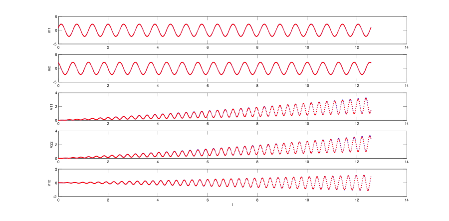
Figure 1: Integration of Example 1. Exact values of $m_{t_{n}},v_{t_{n}}$ and their approximations $\widehat{m}_{t_{n}},\widehat{v}_{t_{n}}$ computed via Monte Carlos with $M=2^{16}$ realizations of the Scheme 1.

Results of Tables 1 and 2, together with Figure 1, indicate that the estimators for the mean and variance of (26) obtained by means of the simulations of the exact solution (27) and Scheme 1 are quite similar. This is an expected result since the first two moments of the linear SDEs and Scheme 1 are ”equal” (up to the precision of the floating-point arithmetic in the numerical computation of the involved exponential and square root matrices).

/$M$	$2^{8}$	$2^{10}$	$2^{12}$	$2^{14}$	$2^{16}$	$2^{18}$
$\widehat{e}^{[1]}$	0.10710	0.05228	0.04536	0.01508	0.00686	0.00275
$\widehat{e}^{[2]}$	0.10643	0.05025	0.04469	0.01433	0.00647	0.00304
$\widehat{e}^{[3]}$	0.43411	0.25916	0.18319	0.29184	0.07244	0.03181
$\widehat{e}^{[4]}$	0.39102	0.29529	0.21413	0.29496	0.07726	0.02753
$\widehat{e}^{[5]}$	0.23859	0.14325	0.15463	0.16961	0.05187	0.02450
$\overline{e}^{[1]}$	0.27037	0.02964	0.02101	0.02108	0.01487	0.00376
$\overline{e}^{[2]}$	0.27626	0.04147	0.02327	0.02227	0.01452	0.00347
$\overline{e}^{[3]}$	0.92465	0.35064	0.18339	0.15513	0.06024	0.02482
$\overline{e}^{[4]}$	0.89503	0.39518	0.17646	0.14678	0.05655	0.02346
$\overline{e}^{[5]}$	0.36642	0.24892	0.10664	0.08899	0.02785	0.01101

Table 1: Values of the errors $\widehat{e}^{[l]}$ and $\overline{e}^{[l]}$ versus number of simulations $M$ in the Example 1.

	$\widehat{e}^{[1]}$	$\widehat{e}^{[2]}$	$\widehat{e}^{[3]}$	$\widehat{e}^{[4]}$	$\widehat{e}^{[5]}$	$\overline{e}^{[1]}$	$\overline{e}^{[2]}$	$\overline{e}^{[3]}$	$\overline{e}^{[4]}$	$\overline{e}^{[5]}$
$\widetilde{\gamma}$	0.52	0.53	0.44	0.44	0.41	0.44	0.44	0.44	0.43	0.45
$std$	0.16	0.16	0.20	0.20	0.21	0.18	0.19	0.21	0.21	0.20

Table 2: Average $\widetilde{\gamma}$ and standard deviation $std$ of the estimators for the rate of convergency $\gamma=1/2$ of the Monte Carlo simulations in the Example 1.

/$M$	$2^{8}$	$2^{10}$	$2^{12}$	$2^{14}$	$2^{16}$	$2^{18}$
$r^{[1]}$	0.0522	0.0177	0.0105	0.0037	0.0016	0.0010
$r^{[2]}$	0.0534	0.0159	0.0106	0.0037	0.0014	0.0010

Table 3: Relative error $r^{[l]}$ in the computation of the functionals $\overline{h}_{\tau_{n}}^{[l]}$ and $\widehat{h}_{\tau_{n}}^{[l]}$ with different number of simulations ${\small M}$ in the Example 1.

In addition, let us compute the relative difference

$$r^{[l]}\left(M\right)=\max_{n}\left\{\left|(\overline{h}_{\tau_{n}}^{[l]}-\widehat{h}_{\tau_{n}}^{[l]})/\overline{h}_{\tau_{n}}^{[l]}\right|\right\}$$

between the approximations

$$\overline{h}_{\tau_{n}}^{[l]}=\frac{1}{M}\sum\limits_{i=1}^{M}\arctan\left(1+\left(\left(X_{\tau_{n}}^{l}\right)^{\{i\}}\right)^{2}\right)\text{ \ \ \ \ \ \ \ and \ \ \ \ \ \ \ }\widehat{h}_{\tau_{n}}^{[l]}=\frac{1}{M}\sum\limits_{i=1}^{M}\arctan\left(1+\left(\left(z_{n}^{l}\right)^{\{i\}}\right)^{2}\right)$$

of the nonlinear functionals $h_{\tau_{n}}^{[l]}=\mathbb{E}\left(\arctan\left(1+(X_{\tau_{n}}^{l})^{2}\right)\right)$, with $l=1,2$. Table 3 displays the values of $r^{[l]}$ for different values of $M$. As it was also expected, $r^{[l]}$ goes to zero as the number of simulations $M$ increases. Furthermore, Table 3 shows that there is no significant difference between the estimates obtained from sampling the exact solution $X_{\tau_{n}}$ and Scheme 1, even though $\mathbb{E}\left(\arctan\left(1+(X_{\tau_{n}}^{l})^{2}\right)\right)$ involves the computation of high order moments of $X_{\tau_{n}}$.

The above simulation results illustrate the feasibility of Scheme 1 for approximating functionals of linear SDEs with multiplicative noise. At this point is worth to mention that, with the uniform time partition consider here, the Euler scheme leads divergent results or computer overflows in the integration of the equation (26).

Example 2.

Nonautonomous nonlinear SDE [16].

$$d\left[\begin{array}[]{c}X_{t}^{1}\\ X_{t}^{2}\end{array}\right]=\left[\begin{array}[]{c}-X_{t}^{2}\\ X_{t}^{1}\end{array}\right]dt+\left[\begin{array}[]{c}0\\ \frac{\sin(X_{t}^{1}+X_{t}^{2})}{\sqrt{1+t}}\end{array}\right]dW_{t}^{1}+\left[\begin{array}[]{c}\frac{\cos(X_{t}^{1}+X_{t}^{2})}{\sqrt{1+t}}\\ 0\end{array}\right]dW_{t}^{2},$$ (30)

with initial condition $(X_{0}^{1},X_{0}^{2})=(1,1)$ and $t\in[0,10]$. For this equation, $E(\phi(X_{t}))=\left|X_{t_{0}}\right|^{2}+\log(1+t)$, with $\phi(X)=\left|X\right|^{2}$.

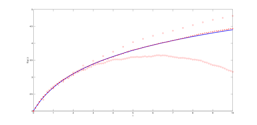
Figure 2: Integration of Example 2. Exact Value: solid line. Scheme 1: $\square$ with $\Delta=0.5$, $+$ with $\Delta=0.25$, $\ast$ with $\Delta=0.1$. Euler with Romberg extrapolation: $o$ with $\Delta=0.05$ and $\Delta=0.1$

It is well-known from [16] that via Monte Carlo simulations: 1) both, the Euler and the Milstein schemes with fixed stepsize $\Delta=0.01$ fail to approximate $E(\phi(X_{t}))$; and 2) the second order method arising from Romberg’s extrapolation of the Euler scheme with stepsizes $0.02$ and $0.01$ gives a satisfactory approximation to $E\left(\phi\left(X_{t}\right)\right)$, but fails when the stepsizes are $0.05$ and $0.1$. Similarly to the fourth figure in [16], Figure 2 illustrates this last result for a Monte Carlo estimation with $M=10000$ simulations.

Figure 2 also shows the computation of $E(\phi(X_{t}))$ via Monte Carlo method and Scheme 1, but on uniform time partitions with stepsizes $\Delta=0.5,0.25,0.1$ and $M=10000$ simulations. In addition, Table 4 provides the estimates $\widehat{e}$ of the mean errors $e=E(\phi(z_{N}))-E(\phi(X_{T}))$ resulting from the integration of (30) via Scheme 1 with different stepsizes. For this, the simulated trajectories $z_{N}^{\{i,j\}}$, $i=1,...,K$ and $j=1,...,M$, were are arranged into $K=100$ batches of $M=10000$ trajectories each for computing

$$\text{\ }\widehat{e}=\frac{1}{K}\sum\limits_{j=1}^{K}\widehat{e}_{j}\text{ \ \ \ \ \ \ with \ \ \ \ \ }\widehat{e}_{j}=\frac{1}{M}\sum\limits_{i=1}^{M}\phi\left(z_{N}^{\{i,j\}}\right)-E\left(\phi\left(X_{T}\right)\right).\text{ }$$

The $90\%=100(1-\alpha)\%$ confidence interval of the Student’s $t$ distribution with $K-1$ degrees for the mean error is given by

$$[\widehat{e}-\Delta\widehat{e},\widehat{e}+\Delta\widehat{e}],$$

where

$$\Delta\widehat{e}=t_{1-\alpha,K-1}\sqrt{\frac{\widehat{\sigma}_{e}^{2}}{K}},\text{ \ \ \ \ with\ \ \ \ \ \ \ \ \ }\widehat{\sigma}_{e}^{2}=\frac{1}{K-1}\sum\limits_{j=1}^{K}(e_{j}-\widehat{e})^{2}.$$

For comparison, the same estimate of the mean error for Euler scheme is also given in Table 4. This illustrates again the better performance of the Scheme 1 introduced in this paper.

$\widehat{e}/\Delta$	$1$	$0.5$	$0.25$	$0.1$
Scheme 1	$-2.2360\pm 0.0093$	$-0.4512\pm 0.0067$	$-0.0868\pm 0.0054$	$0.0076\pm 0.0053$
Euler	$-2435.8\pm 1.7826$	$-235.05\pm 0.2192$	$-32.031\pm 0.0361$	$-5.7704\pm 0.0101$

Table 4: Estimate $\widehat{e}$ of the mean error $E(\phi(z_{N}))-E(\phi(X_{T}))$ in the integration of (30) by means of Scheme 1 and the Euler scheme for different integration stepsizes $\Delta$.

6 Conclusions

A weak Local Linearization scheme for stochastic differential equations with multiplicative noise was introduced. The scheme preserves the first two moments of the solution of linear SDEs and the mean square stability that such solution may have. The order-1 of weak convergence was proved and the practical performance of the scheme in the evaluation of functionals of linear and nonlinear SDEs was illustrated with numerical simulations. The simulations also showed the significant higher accuracy of the introduced scheme in comparison with the Euler scheme.

Acknowledgement. This work was partially supported by FONDECYT Grant 1140411. CMM was also partially supported by BASAL Grant PFB-03.

References

- [1] Arnold L., Stochastic Differential Equations: Theory and Applications, Wiley-Interscience Publications, New York, 1974.
- [2] Biscay R., Jimenez J.C., Riera J. and Valdes P., Local linearization method for the numerical solution of stochastic differential equations, Annals Inst. Statis. Math., 48 (1996) 631-644.
- [3] Carbonell F., Jimenez J.C. and Biscay R.J., Weak local linear discretizations for stochastic differential equations: convergence and numerical schemes, J. Comput. Appl. Math., 197 (2006) 578-596.
- [4] Golub G.H. and Van Loan C.F., Matrix Computations, 3rd Edition, The Johns Hopkins University Press, 1996.
- [5] Jimenez J.C., Simplified formulas for the mean and variance of linear stochastic differential equations, Appl. Math. Letters, 49 (2015) 12-19.
- [6] Jimenez J.C. and Biscay R., Approximation of continuous time stochastic processes by the Local Linearization method revisited. Stochast. Anal. & Appl., 20 (2002) 105-121.
- [7] Jimenez J.C., Carbonell F., Rate of convergence of local linearization schemes for initial-value problems, Appl. Math. Comput., 171 (2005) 1282-1295.
- [8] Jimenez J.C. and Ozaki T., Linear estimation of continuous-discrete linear state space models with multiplicative noise, Systems & Control Letters, 47 (2002) 91-101.
- [9] Jimenez J.C. and Ozaki T., Local Linearization filters for nonlinear continuous-discrete state space models with multiplicative noise. Int. J. Control, 76 (2003) 1159-1170.
- [10] Kloeden P.E. and Platen E., Numerical Solution of Stochastic Differential Equations, Springer-Verlag, Berlin, Second Edition, 1995.
- [11] Milstein G.N. and Tretyakov M.V., Stochastic Numerics for Mathematical Physics, Springer, 2004.
- [12] Moler C. and Van Loan C., Nineteen dubious ways to compute the exponential of a matrix, SIAM Review, 45 (2003) 3-49.
- [13] Mora C., Numerical solution of conservative finite-dimensional stochastic Schrödinger equations, Ann. Appl. Probab., 15 (2005), 2144-2171.
- [14] Shoji I., A note on convergence rate of a linearization method for the discretization of stochastic differential equations, Commun. Nonlinear Sci. Numer. Simulat. 16 (2011) 2667-2671.
- [15] Stramer, O., The local linearization scheme for nonlinear diffusion models with discontinuous coefficients, Stat. Prob. Letters, 42 (1999) 249-256.
- [16] Talay D. and Tubaro L., Expansion of the global error for numerical schemes solving stochastic differential equations, Stochast. Anal. Appl., 8 (1990) 94-120.