Dependent Multinomial Models Made Easy:
Stick Breaking with the Pólya-Gamma Augmentation

Abstract

Many practical modeling problems involve discrete data that are best represented as draws from multinomial or categorical distributions. For example, nucleotides in a DNA sequence, children’s names in a given state and year, and text documents are all commonly modeled with multinomial distributions. In all of these cases, we expect some form of dependency between the draws: the nucleotide at one position in the DNA strand may depend on the preceding nucleotides, children’s names are highly correlated from year to year, and topics in text may be correlated and dynamic. These dependencies are not naturally captured by the typical Dirichlet-multinomial formulation. Here, we leverage a logistic stick-breaking representation and recent innovations in Pólya-gamma augmentation to reformulate the multinomial distribution in terms of latent variables with jointly Gaussian likelihoods, enabling us to take advantage of a host of Bayesian inference techniques for Gaussian models with minimal overhead.

journalname captionbox copyrightbox CAPcaptionbox

and

t1These authors contributed equally.

1 Introduction

It is often desirable to model discrete data in terms of continuous latent structure. In applications involving text corpora, discrete-valued time series, or polling and purchasing decisions, we may want to learn correlations or spatiotemporal dynamics, and leverage these learned structures to improve inferences and predictions. However, adding these continuous latent dependence structures often comes at the cost of significantly complicating inference: such models may require specialized, one-off inference algorithms, such as a nonconjugate variational optimization, or they may only admit very general inference tools like particle MCMC Andrieu et al. (2010) or elliptical slice sampling Murray et al. (2010), which can be inefficient and difficult to scale. Developing, extending, and applying these models has remained a challenge.

In this paper we aim to provide a class of such models that are easy and efficient. We develop models for categorical and multinomial data in which dependencies among the multinomial parameters are modeled via latent Gaussian distributions or Gaussian processes, and we show that this flexible class of models admits a simple auxiliary variable method that makes inference easy, fast, and modular. This construction not only makes these models simple to develop and apply, but also allows the resulting inference methods to use off-the-shelf algorithms and software for Gaussian processes and linear Gaussian dynamical systems.

The paper is organized as follows. After providing background material and defining our general models and inference methods, we demonstrate the utility of this class of models by applying it to three domains as case studies. First, we develop a correlated topic model for text corpora. Second, we study an application to modeling the spatial and temporal patterns in birth names given only sparse data. Finally, we provide a new continuous state-space model for discrete-valued sequences, including text and human DNA. In each case, given our model construction and auxiliary variable method, inference algorithms are easy to develop and very effective in experiments. We conclude with comments on the new kinds of models these methods may enable.

Code to use these models and reproduce all the figures is available at https://github.com/HIPS/pgmult.

2 Modeling correlations in multinomial parameters

In this section, we discuss an auxiliary variable scheme that allows multinomial observations to appear as Gaussian likelihoods within a larger probabilistic model. The key trick discussed in the proceeding sections is to introduce Pólya-gamma random variables into the joint distribution over data and parameters in such a way that the resulting marginal leaves the original model intact.

2.1 Pólya-gamma augmentation

The integral identity at the heart of the Pólya-gamma augmentation scheme Polson et al. (2013) is

$$\frac{(e^{\psi})^{a}}{(1+e^{\psi})^{b}}=2^{-b}e^{\kappa\psi}\int_{0}^{\infty}e^{-\omega\psi^{2}/2}p(\omega\,|\,b,0)\,\mathrm{d}\omega,$$ (1)

where ${\kappa=a-b/2}$ and $p(\omega\,|\,b,0)$ is the density of the Pólya-gamma distribution ${\mathrm{PG}(b,0)}$, which does not depend on $\psi$. Consider a likelihood function of the form

$$p(x\,|\,\psi)=c(x)\frac{(e^{\psi})^{a(x)}}{(1+e^{\psi})^{b(x)}}$$ (2)

for some functions $a$, $b$, and $c$. Such likelihoods arise, e.g., in logistic regression and in binomial and negative binomial regression Polson et al. (2013). Using (1) along with a prior $p(\psi)$, we can write the joint density of $(\psi,x)$ as

$$p(\psi,x)=p(\psi)\,c(x)\frac{(e^{\psi})^{a(x)}}{(1+e^{\psi})^{b(x)}}=\int_{0}^{\infty}p(\psi)\,c(x)\,2^{-b(x)}e^{\kappa(x)\psi}e^{-\omega\psi^{2}/2}p(\omega\,|\,b(x),0)\;\mathrm{d}\omega.$$ (3)

The integrand of (3) defines a joint density on $(\psi,x,\omega)$ which admits $p(\psi,x)$ as a marginal density. Conditioned on these auxiliary variables $\omega$, we have

$$p(\psi\,|\,x,\omega)\propto p(\psi)e^{\kappa(x)\psi}e^{-\omega\psi^{2}/2}$$ (4)

which is Gaussian when $p(\psi)$ is Gaussian. Furthermore, by the exponential tilting property of the Pólya-gamma distribution, we have ${\omega\,|\,\psi,x\sim\mathrm{PG}(b(x),\psi)}$. Thus the identity (1) gives rise to a conditionally conjugate augmentation scheme for Gaussian priors and likelihoods of the form (2).

This augmentation scheme has been used to develop Gibbs sampling and variational inference algorithms for Bernoulli, binomial Polson et al. (2013), and negative binomial regression models Zhou et al. (2012) with logit link functions. In this paper we extend it to the multinomial distribution.

2.2 A Pólya-gamma augmentation for the multinomial distribution

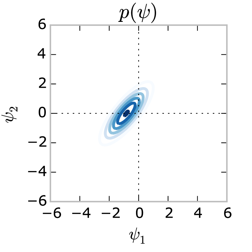
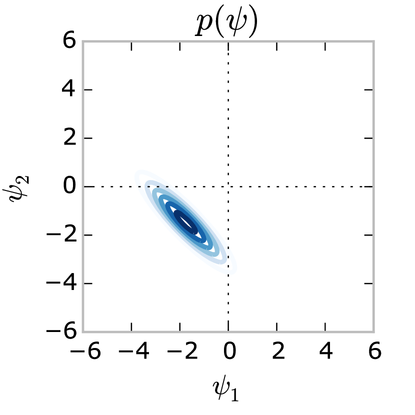
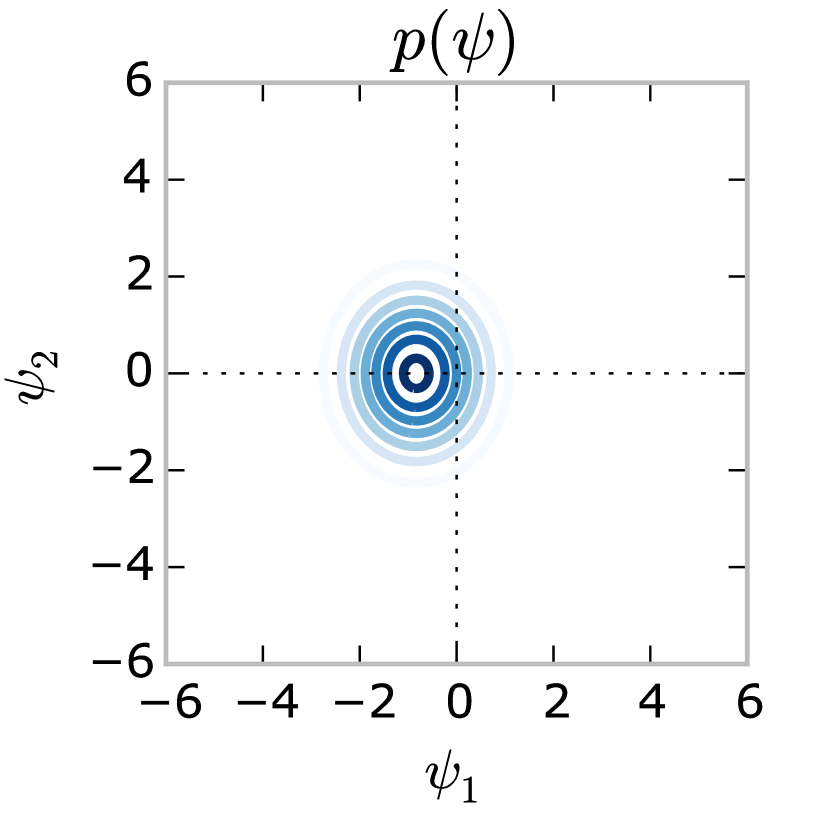
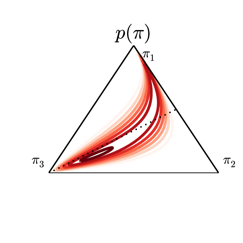
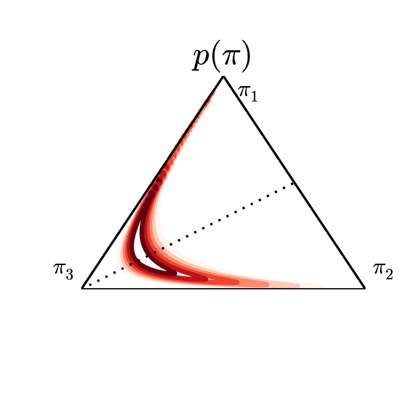
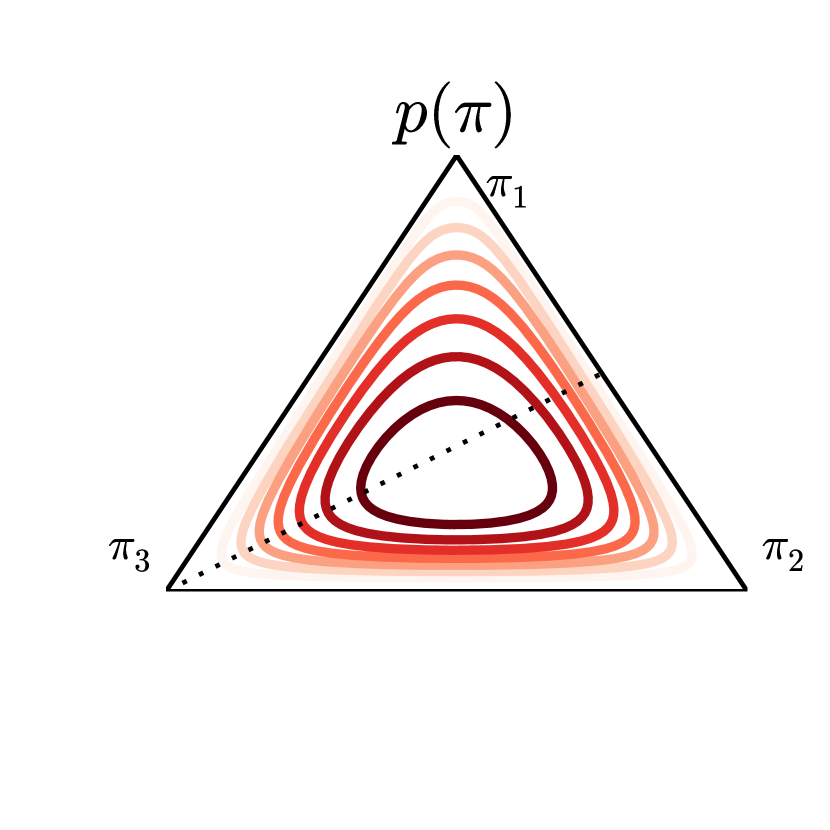
Figure 1: Correlated 2D Gaussian priors on $\boldsymbol{\psi}$ and their implied densities on $\pi_{\mathsf{SB}}(\boldsymbol{\psi})$. See text for details.

To develop a Pólya-gamma augmentation for the multinomial, we first rewrite the $K$-dimensional multinomial density recursively in terms of ${K-1}$ binomial densities:

$$\mathrm{Mult}(\boldsymbol{x}\,|\,N,\boldsymbol{\pi})=\prod_{k=1}^{K-1}\mathrm{Bin}(x_{k}\,|\,N_{k},\widetilde{\pi}_{k}),$$ (5)

$$N_{k}=N-\sum_{j<k}x_{j},\quad\widetilde{\pi}_{k}=\frac{\pi_{k}}{1-\sum_{j<k}\pi_{j}},\quad k=2,3,\ldots,K,$$ (6)

where $N_{1}=N=\sum_{k}x_{k}$ and $\widetilde{\pi}_{1}=\pi_{1}$. For convenience, we define ${N(\boldsymbol{x})\equiv\left[N_{1},\ldots,N_{K-1}\right]}$. This decomposition of the multinomial density is a “stick-breaking” representation where each $\widetilde{\pi}_{k}$ represents the fraction of the remaining probability mass assigned to the $k$-th component. We let $\widetilde{\pi}_{k}=\sigma(\psi_{k})$ and define the function, ${\pi_{\mathsf{SB}}:\mathbb{R}^{K-1}\to[0,1]^{K}}$, which maps a vector $\boldsymbol{\psi}$ to a normalized probability vector $\boldsymbol{\pi}$.

Next, we rewrite the density into the form required by (1) by substituting $\sigma(\psi_{k})$ for $\widetilde{\pi}_{k}$:

$$\mathrm{Mult}(\boldsymbol{x}\,|\,N,\boldsymbol{\psi})=\prod_{k=1}^{K-1}\mathrm{Bin}(x_{k}\,|\,N_{k},\sigma(\psi_{k})) =\prod_{k=1}^{K-1}{N_{k}\choose x_{k}}\sigma(\psi_{k})^{x_{k}}(1-\sigma(\psi_{k}))^{N_{k}-x_{k}}$$ (7)

$$=\prod_{k=1}^{K-1}{N_{k}\choose x_{k}}\frac{(e^{\psi_{k}})^{x_{k}}}{(1+e^{\psi_{k}})^{N_{k}}}.$$ (8)

Choosing ${a_{k}(x)=x_{k}}$ and ${b_{k}(x)=N_{k}}$ for each ${k=1,2,\ldots,K-1}$, we can then introduce Pólya-gamma auxiliary variables $\omega_{k}$ corresponding to each coordinate $\psi_{k}$; dropping terms that do not depend on $\boldsymbol{\psi}$ and completing the square yields

$$p(\boldsymbol{x},\boldsymbol{\omega}\,|\,\boldsymbol{\psi})\propto\prod_{k=1}^{K-1}e^{(x_{k}-N_{k}/2)\psi_{k}-\omega_{k}\psi_{k}^{2}/2} \propto\mathcal{N}\left(\boldsymbol{\psi}\,\bigg{|}\,\boldsymbol{\Omega}^{-1}\kappa(\boldsymbol{x}),\,\boldsymbol{\Omega}^{-1}\right),$$ (9)

where ${\boldsymbol{\Omega}\equiv\text{diag}(\boldsymbol{\omega})}$ and ${\kappa(\boldsymbol{x})\equiv\boldsymbol{x}-N(\boldsymbol{x})/2}$. That is, conditioned on $\boldsymbol{\omega}$, the likelihood of $\boldsymbol{\psi}$ under the augmented multinomial model is proportional to a diagonal Gaussian distribution.

Figure 1 illustrates how a variety of Gaussian densities map to probability densities on the simplex. Correlated Gaussians (left) put most probability mass near the $\pi_{1}=\pi_{2}$ axis of the simplex, and anti-correlated Gaussians (center) put mass along the sides where $\pi_{1}$ is large when $\pi_{2}$ is small and vice-versa. Finally, a nearly spherical Gaussian approximates a symmetric Dirichlet distribution. Appendix A derives a closed-form expression for the density on $\boldsymbol{\pi}$ implied by a Gaussian distribution on $\boldsymbol{\psi}$, as well an expression for a diagonal Guassian distribution that best approximates, in a moment-matching sense, a Dirichlet distribution on $\boldsymbol{\pi}$.

2.3 Alternative models

This stick breaking transformation has been explored in the previous work of Ren et al. (2011) and Khan et al. (2012), but has not been connected with the Pólya-gamma augmentation. The multinomial probit and logistic normal methods are most commonly used, and we describe them here.

The multinomial probit model Albert and Chib (1993) applies to categorical regrssion, and is based upon the following auxiliary variable model: ${z_{k}=\Phi(\psi_{k}+\epsilon_{k})}$, where $\Phi$ is the probit function and $\epsilon_{k}\sim\mathcal{N}(0,1)$. Given these auxiliary variables, ${x_{k}=1}$ if ${z_{k}>z_{j}\,\forall j\neq k}$, and ${x_{k}=0}$ otherwise. This approach has primarily focused on categorical modeling.

A common method of modeling correlated multinomial parameters, to which we directly compare in the following sections, is based on the “softmax” or multi-class logistic function, ${\pi_{k}=e^{\psi_{k}}/\sum_{j=1}^{K}e^{\psi_{j}}}$. Let $\pi_{\mathsf{LN}}:\mathbb{R}^{K}\to[0,1]^{K}$ denote the joint transformation. This has found application in multiclass regression Holmes et al. (2006) and is the common approach to correlated topic modeling Blei and Lafferty (2006a). However, leveraging this transformation in conjunction with Gaussian models for $\boldsymbol{\psi}$ is challenging due to the lack of conjugacy, and previous work has relied upon variational approximations to tackle the hard inference problem Blei and Lafferty (2006a).

Unlike the logistic normal and multinomial probit, the stick-breaking transformation we employ is asymmetric. Our illustrations in Figure 1 and the discussion in Appendix A show that this lack of symmetry does not impair the representational capacity of the model.

3 Correlated topic models

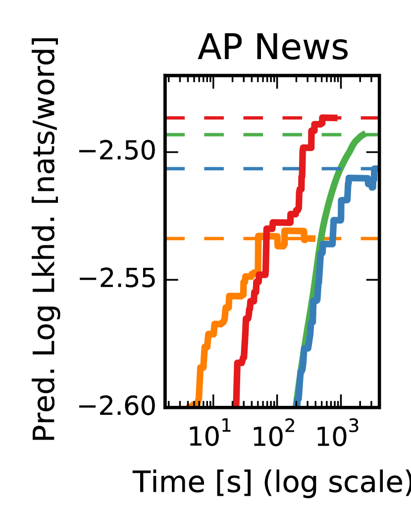
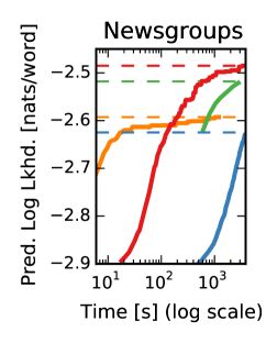
Figure 2: A comparison of correlated topic model performance. The left panel shows a subset of the inferred topic correlations for the AP News corpus. Two examples are highlighted: a) positive correlation between topics (house, committee, congress, law) and (Bush, Dukakis, president, campaign), and b) anticorrelation between (percent, year, billion, rate) and (court, case, attorney, judge). The middle and right panels demonstrate the efficacy of our SB-CTM relative to competing models on the AP News corpus and the 20 Newsgroup corpus, respectively.

The Latent Dirichlet Allocation (LDA) (Blei et al., 2003) is a popular model for learning topics from text corpora. The Correlated Topic Model (CTM) (Blei and Lafferty, 2006a) extends LDA by including a Gaussian correlation structure among topics. This correlation model is powerful not only because it reveals correlations among topics but also because inferring such correlations can significantly improve predictions, especially when inferring the remaining words in a document after only a few have been revealed Blei and Lafferty (2006a). However, the addition of this Gaussian correlation structure breaks the Dirichlet-Multinomial conjugacy of LDA, making estimation and particularly Bayesian inference and model-averaged predictions more challenging. An approximate maximum likelihood approach using variational EM Blei and Lafferty (2006a) is often effective, but a fully Bayesian approach which integrates out parameters may be preferable, especially when making predictions based on a small number of revealed words in a document. A recent Bayesian approach based on a Pólya-Gamma augmentation to the logistic normal CTM (LN-CTM) Chen et al. (2013) provides a Gibbs sampling algorithm with conjugate updates, but the Gibbs updates are limited to single-site resampling of one scalar at a time, which can lead to slow mixing in correlated models.

In this section we show that MCMC sampling in a correlated topic model based on the stick breaking construction (SB-CTM) can be significantly more efficient than sampling in the LN-CTM while maintaining the same integration advantage over EM.

In the standard LDA model, each topic $\boldsymbol{\beta}_{t}$ ($t=1,2,\ldots,T$) is a distribution over a vocabulary of $V$ possible words, and each document $d$ has a distribution over topics $\boldsymbol{\theta}_{d}$ ($d=1,2,\ldots,D$). The $n$th word in document $d$ is denoted $w_{n,d}$ for $d=1,2,\ldots,N_{d}$. When each $\boldsymbol{\beta}_{t}$ and $\boldsymbol{\theta}_{d}$ is given a symmetric Dirichlet prior with concentration parameters $\alpha_{\beta}$ and $\alpha_{\theta}$, respectively, the full generative model is

$$\boldsymbol{\beta}_{t}\sim\mathrm{Dir}(\alpha_{\beta}),\quad\boldsymbol{\theta}_{d}\sim\mathrm{Dir}(\alpha_{\theta}),\quad z_{n,d}\,|\,\boldsymbol{\theta}_{d}\sim\mathrm{Cat}(\boldsymbol{\theta}_{d}),\quad w_{n,d}\,|\,z_{n,d},\{\boldsymbol{\beta}_{t}\}\sim\mathrm{Cat}(\boldsymbol{\beta}_{z_{n,d}}).$$ (10)

The CTM replaces the Dirichlet prior on each $\boldsymbol{\theta}_{d}$ with a new prior that models the coordinates of $\boldsymbol{\theta}_{d}$ as mutually correlated. This correlation structure on $\boldsymbol{\theta}_{d}$ is induced by first sampling a correlated Gaussian vector $\boldsymbol{\psi}_{d}$ and then applying the logistic normal map:

$$\boldsymbol{\psi}_{d}\,|\,\boldsymbol{\mu},\boldsymbol{\Sigma}\sim\mathcal{N}(\boldsymbol{\mu},\boldsymbol{\Sigma}),\quad\boldsymbol{\theta}_{d}=\pi_{\mathsf{LN}}(\boldsymbol{\psi}_{d})$$ (11)

where the Gaussian parameters $(\boldsymbol{\mu},\boldsymbol{\Sigma})$ can be given a conjugate normal-inverse Wishart (NIW) prior. Analogously, our SB-CTM generates the correlation structure by instead applying the stick-breaking logistic map:

$$\boldsymbol{\psi}_{d}\,|\,\boldsymbol{\mu},\boldsymbol{\Sigma}\sim\mathcal{N}(\boldsymbol{\mu},\boldsymbol{\Sigma}),\quad\boldsymbol{\theta}_{d}=\pi_{\mathsf{SB}}(\boldsymbol{\psi}_{d}).$$ (12)

The goal is then to infer the posterior distribution over the topics $\boldsymbol{\beta}_{t}$, the documents’ topic allocations $\boldsymbol{\psi}_{d}$, and their mean and correlation structure $(\boldsymbol{\mu},\boldsymbol{\Sigma})$. (In the case of the EM algorithm of Blei and Lafferty (2006a), the task is to approximate maximum likelihood estimates of the same parameters.) Modeling correlation structure within the topics $\boldsymbol{\beta}$ can be done analogously.

For fully Bayesian MCMC inference in the SB-CTM, we develop a Gibbs sampler that exploits the block conditional Gaussian structure provided by the stick-breaking construction. The Gibbs sampler iteratively samples ${\boldsymbol{z}\,|\,\boldsymbol{w},\boldsymbol{\beta},\boldsymbol{\psi}}$;   ${\boldsymbol{\beta}\,|\,\boldsymbol{z},\boldsymbol{w}}$;   ${\boldsymbol{\psi}\,|\,\boldsymbol{z},\boldsymbol{\mu},\boldsymbol{\Sigma},\boldsymbol{\omega}}$;   and $\boldsymbol{\mu},\boldsymbol{\Sigma}\,|\,\boldsymbol{\psi}$; as well as the auxiliary variables $\boldsymbol{\omega}\,|\,\boldsymbol{\psi},\boldsymbol{z}$. The first two are standard updates for LDA models, so we focus on the latter three. Using the identities derived in Section 2.2, the conditional density of each $\boldsymbol{\psi}_{d}\,|\,\boldsymbol{z}_{d},\boldsymbol{\mu},\boldsymbol{\Sigma},\boldsymbol{\omega}$ can be written

$$p(\boldsymbol{\psi}_{d}\,|\,\boldsymbol{z}_{d},\boldsymbol{\omega}_{d})\;\propto\;\mathcal{N}(\boldsymbol{\psi}\,|\,\kappa(\boldsymbol{c}_{d}),\boldsymbol{\Omega}_{d}^{-1})\;\mathcal{N}(\boldsymbol{\psi}\,|\,\boldsymbol{\mu},\boldsymbol{\Sigma})\;\propto\;\mathcal{N}(\boldsymbol{\psi}_{d}\,|\,\widetilde{\boldsymbol{\mu}},\widetilde{\boldsymbol{\Sigma}}),$$ (13)

where

$$\widetilde{\boldsymbol{\mu}}=\widetilde{\boldsymbol{\Sigma}}\left[\kappa(\boldsymbol{c}_{d})+\boldsymbol{\Sigma}^{-1}\boldsymbol{\mu}\right],\quad\widetilde{\boldsymbol{\Sigma}}=\left[\boldsymbol{\Omega}_{d}+\boldsymbol{\Sigma}^{-1}\right]^{-1},\quad c_{d,t}=\sum_{n}\mathbb{I}[z_{n,d}=t],\quad\boldsymbol{\Omega}_{d}=\text{diag}(\boldsymbol{\omega}_{d}),$$ (14)

and so it is resampled as a joint Gaussian. The correlation structure parameters $\boldsymbol{\mu}$ and $\boldsymbol{\Sigma}$ with a conjugate NIW prior are sampled from their conditional NIW distribution. Finally, the auxiliary variables $\boldsymbol{\omega}$ are sampled as Pólya-Gamma random variables, with $\boldsymbol{\omega}_{d}\,|\,\boldsymbol{z}_{d},\boldsymbol{\psi}_{d}\sim\mathrm{PG}(N(\boldsymbol{c}_{d}),\boldsymbol{\psi}_{d})$. A feature of the stick-breaking construction is that the the auxiliary variable update can be performed in an embarrassingly parallel computation.

We compare the performance of this Gibbs sampling algorithm for the SB-CTM to the Gibbs sampling algorithm of the LN-CTM Chen et al. (2013), which uses a different Pólya-gamma augmentation, as well as the original variational EM algorithm for the CTM and collapsed Gibbs sampling in standard LDA. Figure 2 shows results on both the AP News dataset and the 20 Newsgroups dataset, where models were trained on a random subset of 95% of the complete documents and tested on the remaining 5% by estimating held-out likelihoods of half the words given the other half. The collapsed Gibbs sampler for LDA is fast but because it does not model correlations its ability to predict is significantly constrained. The variational EM algorithm for the CTM is reasonably fast but its point estimate doesn’t quite match the performance from integrating out parameters via MCMC in this setting. The LN-CTM Gibbs sampler continues to improve slowly but is limited by its single-site updates, while the SB-CTM sampler seems to both mix effectively and execute efficiently due to its block Gaussian updating.

The SB-CTM demonstrates that the stick-breaking construction and corresponding Pólya-Gamma augmentation makes inference in correlated topic models both easy to implement and computationally efficient. The block conditional Gaussianity also makes inference algorithms modular and compositional: the construction immediately extends to dynamic topic models (DTMs) Blei and Lafferty (2006b), in which the latent $\boldsymbol{\psi}_{d}$ evolve according to linear Gaussian dynamics, and inference can be implemented simply by applying off-the-shelf code for Gaussian linear dynamical systems (see Section 5). Finally, because LDA is so commonly used as a component of other models (e.g. for images Wang and Grimson (2008)), easy, effective, modular inference for CTMs and DTMs is a promising general tool.

To apply correlated topic models to increasingly large datasets, a stochastic variational inference (SVI) (Hoffman et al., 2013) approach is promising. In Appendix C, we show that the stick-breaking construction enables an algorithm based on the Pólya-gamma augmentation that can work with subsets, or mini-batches, of data in each iteration. As with the Gibbs sampler, the conditionally conjugate structure makes the algorithm easy to derive and implement.

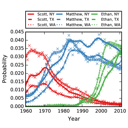
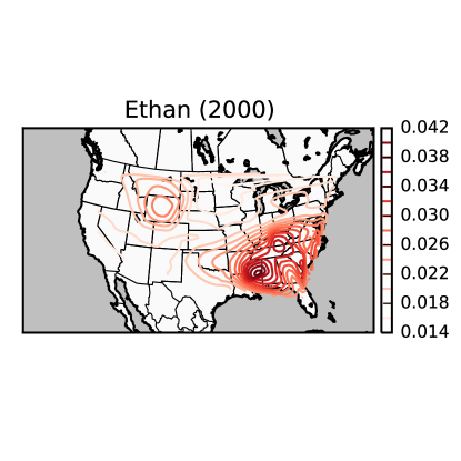
	2012		2013
Model	Top 10	Bot. 10	Top 10	Bot. 10
Static 2011	4.2 (1.3)	0.7 (1.2)	4.2 (1.4)	0.8 (1.0)
Raw GP	4.9 (1.1)	0.7 (0.9)	5.0 (1.0)	0.8 (0.9)
LNM GP	6.7 (1.4)	4.8 (1.7)	6.8 (1.4)	4.6 (1.7)
SBM GP	7.3 (1.0)	4.0 (1.8)	7.0 (1.0)	3.9 (1.4)

Average number of names correctly predicted

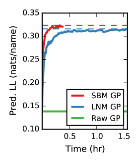
Figure 3: A spatiotemporal Gaussian process applied to the names of children born in the United States from 1960-2013. With a limited dataset of only 50 observations per state/year, the stick breaking and logistic normal multinomial GPs (SBM-GP and LNM-GP) outperform naïve approaches in predicting the top and bottom 10 names (bottom left, parentheses: std. error). Our SBM-GP, which leverages the Pólya-gamma augmentation, is considerably more efficient than the non conjugate LNM-GP (bottom right).

4 Gaussian processes with multinomial observations

Consider the United States census data, which lists the first names of children born in each state for the years 1910-2013. Suppose we wish to predict the probability of a particular name in New York State in the years 2012 and 2013 given observed names in earlier years. We might reasonably expect that name probabilities vary smoothly over time as names rise and fall in popularity, and that name probability would be similar in neighboring states. A Gaussian process naturally captures these prior intuitions about spatiotemporal correlations, but the observed name counts are most naturally modeled as multinomial draws from latent probability distributions over names for each combination of state and year. We show how efficient inference can be performed in this otherwise difficult model by leveraging the Pólya-gamma augmentation.

Let $\boldsymbol{Z}\in\mathbb{R}^{M\times D}$ denote the matrix of $D$ dimensional inputs and $\boldsymbol{X}\in\mathbb{N}^{M\times K}$ denote the observed $K$ dimensional count vectors for each input. In our example, each row $\boldsymbol{z}_{m}$ of $\boldsymbol{Z}$ corresponds to the year, latitude, and longitude of an observation, and $K$ is the number of names. Underlying these observations we introduce a set of latent variables, $\psi_{m,k}$ such that the probability vector at input $\boldsymbol{z}_{m}$ is $\boldsymbol{\pi}_{m}=\pi_{\mathsf{SB}}(\boldsymbol{\psi}_{m,:})$. The auxiliary variables for the $k$-th name, $\boldsymbol{\psi}_{:,k}$, are linked via a Gaussian process with covariance matrix, $\boldsymbol{C}$, whose entry $C_{i,j}$ is the covariance between input $\boldsymbol{z}_{i}$ and $\boldsymbol{z}_{j}$ under the GP prior, and mean vector $\boldsymbol{\mu}_{k}$. The covariance matrix is shared by all names, and the mean is empirically set to match the measured name probability. The full model is then,

$$\boldsymbol{\psi}_{:,k} \sim\mathcal{GP}(\boldsymbol{\mu}_{k},\boldsymbol{C}) \text{ for }k\in\{1,\ldots,K-1\}$$

$$\boldsymbol{x}_{m} \sim\mathrm{Mult}(N_{m},\pi_{\mathsf{SB}}(\boldsymbol{\psi}_{m,:})) \text{ for }m\in\{1,\ldots,M\}.$$

To perform inference, introduce auxiliary Pólya-gamma variables, $\omega_{m,k}$ for each $\psi_{m,k}$. Conditioned on these variables, the conditional distribution of $\boldsymbol{\psi}_{:,k}$ is,

$$\boldsymbol{\psi}_{:,k}\,|\,\boldsymbol{Z},\boldsymbol{X},\boldsymbol{\omega},\boldsymbol{\mu},\boldsymbol{C}\propto\mathcal{N}\left(\boldsymbol{\psi}_{:,k}\,\bigg{|}\,\boldsymbol{\Omega}_{k}^{-1}\kappa(\boldsymbol{X}_{:,k}),\,\boldsymbol{\Omega}_{k}^{-1}\right)\mathcal{N}(\boldsymbol{\psi}_{:,k}\,|\,\boldsymbol{\mu}_{k},\boldsymbol{C})\propto\mathcal{N}\left(\boldsymbol{\psi}_{:,k}\,|\,\widetilde{\boldsymbol{\mu}}_{k},\widetilde{\boldsymbol{\Sigma}}_{k}\right)$$

$$\widetilde{\boldsymbol{\Sigma}}_{k}=\left(\boldsymbol{C}^{-1}+\boldsymbol{\Omega}_{k}\right)^{-1}\qquad\widetilde{\boldsymbol{\mu}}_{k}=\widetilde{\boldsymbol{\Sigma}}_{k}\left(\boldsymbol{C}^{-1}\boldsymbol{\mu}_{k}+\kappa(\boldsymbol{X}_{:,k})\right),$$

where $\boldsymbol{\Omega}_{k}=\text{diag}(\boldsymbol{\omega}_{:,k})$. The auxiliary variables are updated according to their conditional distribution: $\omega_{m,k}\,|\,\boldsymbol{x}_{m},\psi_{m,k}\sim\mathrm{PG}(N_{m,k},\psi_{m,k})$, where $N_{m,k}=N_{m}-\sum_{j<k}x_{m,j}$.

Figure 3 illustrates the power of this approach on U.S. census data. The top two plots show the inferred probabilities under our stick-breaking multinomial GP model for the full dataset. Interesting spatiotemporal correlations in name probability are uncovered. In this large-count regime, the posterior uncertainty is negligible since we observe thousands of names per state and year, and simply modeling the transformed empirical probabilities with a GP works well. However, in the sparse data regime with only ${N_{m}=50}$ observations per input, it greatly improves performance to model uncertainty in the latent probabilities using a Gaussian process with multinomial observations.

The bottom panels compare four methods of predicting future names in the years 2012 and 2013 for a down-sampled dataset with ${N_{m}=50}$: predicting based on the empirical probability measured in 2011; a standard GP to the empirical probabilities transformed by $\pi_{\mathsf{SB}}^{-1}$ (Raw GP); a GP whose outputs are transformed by the logistic normal function, $\pi_{\mathsf{LN}}$, to obtain multinomial probabilities (LNM GP) fit using elliptical slice sampling Murray et al. (2010); and our stick-breaking multinomial GP (SBM GP). In terms of ability to predict the top and bottom 10 names, the multinomial models are both comparable and vastly superior to the naive approaches.

In terms of efficiency, our model is considerably faster than the logistic normal version, as shown in the bottom right panel. This difference is due to two reasons. First, our augmented Gibbs sampler is more efficient than the elliptical slice sampling algorithm used to handle the nonconjugacy in the LNM GP. Second, and perhaps most important, we are able to make collapsed predictions in which we compute the predictive distribution test $\boldsymbol{\psi}$’s given $\boldsymbol{\omega}$, integrating out the training $\boldsymbol{\psi}$. In contrast, the LNM-GP must condition on the training GP values in order to make predictions, and effectively integrate over training samples using MCMC. Appendix B goes into greater detail on how marginal predictions are computed and why they are more efficient than predicting conditioned on a single value of $\boldsymbol{\psi}$.

5 Multinomial linear dynamical systems

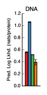
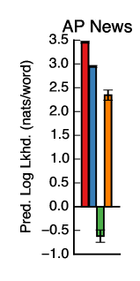
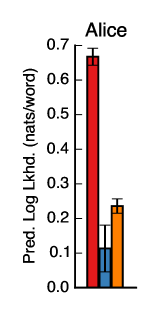
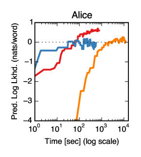
Figure 4: Predictive log likelihood comparison of time series models with multinomial observations.

While discrete-state hidden Markov models (HMMs) are ubiquitous for modeling time series and sequence data, it can be preferable to use a continuous state space model. In particular, while discrete states have no intrinsic structure, continuous states can correspond to a natural embedding or geometry Belanger and Kakade (2015). These considerations are particularly relevant to text, where word embeddings Collobert and Weston (2008) have proven to be a powerful tool.

Gaussian linear dynamical systems (LDS) provide very efficient learning and inference algorithms, but they can typically only be applied when the observations are themselves linear with Gaussian noise. While it is possible to apply a Gaussian LDS to count vectors Belanger and Kakade (2015), the resulting model is misspecified in the sense that, as a continuous density, the model assigns zero probability to training and test data. However, Belanger and Kakade (2015) show that this model can still be used for several machine learning tasks with compelling performance, and that the efficient algorithms afforded by the misspecified Gaussian assumptions confer a significant computational advantage. Indeed, the authors have observed that such a Gaussian model is “worth exploring, since multinomial models with softmax link functions prevent closed-form M step updates and require expensive” computations Belanger and Kakade (2014); this paper aims to help bridge precisely this gap and enable efficient Gaussian LDS computational methods to be applied while maintaining multinomial emissions and an asymptotically unbiased representation of the posteiror. While there are other approximation schemes that effectively extend some of the benefits of LDSs to nonlinear, non-Gaussian settings, such as the extended Kalman filter (EKF) and unscented Kalman filter (UKF) Wan and Van Der Merwe (2000); Thrun et al. (2005), these methods do not allow for asymptotically unbiased Bayesian inference and can have complex behavior. Alternatively, particle MCMC (pMCMC) Andrieu et al. (2010) with ancestor resampling Lindsten et al. (2012) is a very powerful algorithm that provides unbiased Bayesian inference for very general state space models, but it does not enjoy the efficient block updates or conjugacy of LDSs or HMMs.

In this section we show how to use the stick-breaking construction and its Pólya-gamma augmentation to perform efficient inference in LDS with multinomial emissions. We focus on a Gibbs sampler with fully conjugate updates that utilizes standard LDS message passing for efficient block updates.

The stick-breaking multinomial linear dynamical system (SBM-LDS) generates states according to a standard linear Gaussian dynamical system but generates multinomial observations using the stick-breaking logistic map:

$$\boldsymbol{z}_{0}|\boldsymbol{\mu}_{0},\boldsymbol{\Sigma}_{0}\sim\mathcal{N}(\boldsymbol{\mu}_{0},\boldsymbol{\Sigma}_{0}),\quad\boldsymbol{z}_{t}|\boldsymbol{z}_{t-1},\boldsymbol{A},\boldsymbol{B}\sim\mathcal{N}(\boldsymbol{A}\boldsymbol{z}_{t-1},\boldsymbol{B}),\quad\boldsymbol{x}_{t}|\boldsymbol{z}_{t},\boldsymbol{C}\sim\mathrm{Mult}(N_{t},\pi_{\mathsf{SB}}(\boldsymbol{C}\boldsymbol{z}_{t})),$$

where $\boldsymbol{z}_{t}\in\mathbb{R}^{D}$ is the system state at time $t$ and $\boldsymbol{x}_{t}\in\mathbb{N}^{K}$ are the multinomial observations. We suppress notation for conditioning on $\boldsymbol{A}$, $\boldsymbol{B}$, $\boldsymbol{C}$, $\boldsymbol{\mu}_{0}$, and $\boldsymbol{\Sigma}_{0}$, which are system parameters of appropriate sizes that are given conjugate priors. The logistic normal multinomial LDS (LNM-LDS) is defined analogously but uses $\pi_{\mathsf{LN}}$ in place of $\pi_{\mathsf{SB}}$.

To produce a Gibbs sampler with fully conjugate updates, we augment the observations with Pólya-gamma random variables $\omega_{t,k}$. As a result, the conditional state sequence $\boldsymbol{z}_{1:T}|\boldsymbol{\omega}_{1:T},\boldsymbol{x}_{1:T}$ is jointly distributed according to a Gaussian LDS in which the diagonal observation potential at time $t$ is $\mathcal{N}(\boldsymbol{\Omega}_{t}^{-1}\kappa(\boldsymbol{x}_{t})|\boldsymbol{C}\boldsymbol{z}_{t},\boldsymbol{\Omega}_{t}^{-1})$; because the observation potential is diagonal, this block update can be performed in only $\mathcal{O}(TD^{3}+TD^{2}K)$ time, and so these updates can be scaled efficiently to large observation dimension $K$. Thus the state sequence can be jointly sampled using off-the-shelf LDS software, and the system parameters can similarly be updated using standard algorithms. The only remaining update is to the auxiliary variables, which are sampled according to ${\boldsymbol{\omega}_{t}|\boldsymbol{z}_{t},\boldsymbol{C},\boldsymbol{x}\sim\mathrm{PG}(N(\boldsymbol{x}_{t}),\boldsymbol{C}\boldsymbol{z}_{t})}$.

We compare the SBM-LDS and the Gibbs sampling inference algorithm to three baseline methods: an LNM-LDS using pMCMC and ancestor resampling for inference, an HMM using Gibbs sampling, and a “raw” LDS which treats the multinomial observation vectors as observations in $\mathbb{R}^{K}$, as in Belanger and Kakade (2015). We examine each method’s performance on each of three experiments: in modeling a sequence of 682 amino acids from human DNA with 22 dimensional observations, a set of 20 random AP news articles with an average of 77 words per article and a vocabulary size of 200 words, and an excerpt of 4000 words from Lewis Carroll’s Alice’s Adventures in Wonderland with a vocabulary of 1000 words. We reserved the final 10 amino acids, 10 words per news article, and 100 words from Alice for computing predictive likelihoods. Each linear dynamical model had a 10-dimensional state space, while the HMM had 10 discrete states (HMMs with 20, 30, and 40 states all performed worse on these tasks).

Figure 4 (left panels) shows the predictive log likelihood for each method on each experiment, normalized by the number of counts in the test dataset and setting to zero the likelihood under a multinomial model fit to the training data mean. For the DNA data, which has the smallest “vocabulary” size, the HMM achieves the highest predictive likelihood, but the SBM-LDS edges out the other LDS methods. On the two text datasets, the SBM-LDS outperforms the other methods, particularly in Alice where the vocabulary is larger and the document is longer. In terms of run time, the SBM-LDS is orders of magnitude faster than the LNM-LDS with pMCMC (right panel) because it mixes much more efficiently over the latent trajectories.

The SBM-LDS is an easy but powerful linear state space model for multinomial observations. The Gibbs sampler leveraging the Pólya-gamma augmentation appears very efficient, performing comparably to an optimized HMM implementation and orders of magnitude faster than a general pMCMC algorithm. Because the augmentation renders the states’ conditional distribution a Gaussian LDS, it easily interfaces with high-performance LDS software, and extending these models with additional structure or covariates can be similarly modular.

6 Related Work

The stick-breaking transformation used herein was applied to categorical models by Khan et al. (2012), but they used local variational bound instead of the Pólya-gamma augmentation. Their promising results corroborate our findings of improved performance using this transformation. Their generalized expectation-maximization algorithm is not fully Bayesian, and does not integrate into existing Gaussian modeling code as easily as our augmentation.

Conversely, Chen et al. (2013) used the Pólya-gamma augmentation in conjunction with the logistic normal transformation for correlated topic modeling, exploiting the conditional conjugacy of a single entry ${\psi_{k}\,|\,\omega_{k},\boldsymbol{\psi}_{\neg k}}$ with a Gaussian prior. Unlike our stick-breaking transformation which admits block Gibbs sampling over the entire vector $\boldsymbol{\psi}$ simultaneously, their approach is limited to single-site Gibbs sampling. As shown in our correlated topic model experiments, this has dramatic effects on inferential performance. Moreover, it precludes analytical marginalization and integration with existing Gaussian modeling algorithms. For example, it is not immediately applicable to inference in linear dynamical systems with multinomial observations.

7 Conclusion

These case studies demonstrate that the stick-breaking multinomial model construction paired with the Pólya-gamma augmentation yields a flexible class of models with easy, efficient, and compositional inference. In addition to making these models easy, the methods developed here can also enable new models for multinomial and mixed data: the latent continuous structures used here to model correlations and state-space structure can be leveraged to explore new models for interpretable feature embeddings, interacting time series, and dependence with other covariates.

Acknowledgments

We thank the members of the Harvard Intelligent Probabilistic Systems (HIPS) group, especially Yakir Reshef, for many helpful conversations. S.W.L. is supported by the Center for Brains, Minds and Machines (CBMM), funded by NSF STC award CCF-1231216. M.J.J. is supported by the Harvard/MIT Joint Research Grants Program. R.P.A. is partially supported by NSF IIS-1421780.

Appendix A Transforming between $p(\boldsymbol{\psi})$ and $p(\boldsymbol{\pi})$

Since the mapping between $\boldsymbol{\pi}$ and $\boldsymbol{\psi}$ is invertible, we can compute the distribution on $\boldsymbol{\pi}$ that is implied by a Gaussian distribution on $\boldsymbol{\psi}$. Assume $\boldsymbol{\psi}\sim\mathcal{N}(\boldsymbol{\mu},\boldsymbol{\Sigma})$. Then,

$$p(\boldsymbol{\pi}\,|\,\boldsymbol{\mu},\boldsymbol{\Sigma}) =\mathcal{N}(\pi_{\mathsf{SB}}^{-1}(\boldsymbol{\pi})\,|\,\boldsymbol{\mu},\boldsymbol{\Sigma})\left|\frac{\mathrm{d}\boldsymbol{\psi}}{\mathrm{d}\boldsymbol{\pi}}\right|$$

From above, we have

$$\psi_{1} =\sigma^{-1}(\pi_{1}), \psi_{2} =\sigma^{-1}\left(\frac{\pi_{2}}{1-\pi_{1}}\right), \ldots, \psi_{k} =\sigma^{-1}\left(\frac{\pi_{k}}{1-\sum_{j<k}\pi_{j}}\right).$$

Let

$$g(x)=\frac{\mathrm{d}\sigma^{-1}(\mathit{x})}{\mathrm{d}\mathit{x}}\bigg{|}_{\mathit{x}=x}=\frac{\mathrm{d}}{\mathrm{d}x}\log\left(\frac{x}{1-x}\right)=\frac{1}{x}+\frac{1}{1-x}=\frac{1}{x(1-x)}.$$

Then,

$$\frac{\partial\psi_{1}}{\partial\pi_{1}} =g(\pi_{1}), \frac{\partial\psi_{k}}{\partial\pi_{k}} =g\left(\frac{\pi_{k}}{1-\sum_{j<k}\pi_{j}}\right)\frac{1}{1-\sum_{j<k}\pi_{j}}, \frac{\partial\psi_{k}}{\partial\pi_{j>k}} =0.$$

Since the Jacobian of the inverse transformation is lower diagonal, its determinant is simply the product of its diagonal,

$$\left|\frac{\mathrm{d}\boldsymbol{\psi}}{\mathrm{d}\boldsymbol{\pi}}\right| =\prod_{k=1}^{K}\left[g\left(\frac{\pi_{k}}{1-\sum_{j<k}\pi_{j}}\right)\frac{1}{1-\sum_{j<k}\pi_{j}}\right]$$

$$=\prod_{k=1}^{K}\left[\frac{1-\sum_{j<k}\pi_{j}}{\pi_{k}}\frac{1-\sum_{j<k}\pi_{j}}{1-\sum_{j<k}\pi_{j}-\pi_{k}}\frac{1}{1-\sum_{j<k}\pi_{j}}\right]$$

$$=\prod_{k=1}^{K}\left[\frac{1-\sum_{j=1}^{k-1}\pi_{j}}{\pi_{k}(1-\sum_{j=1}^{k}\pi_{j})}\right]$$

Thus, the final density is,

$$p(\boldsymbol{\pi}\,|\,\boldsymbol{\mu},\boldsymbol{\Sigma}) =\mathcal{N}(\pi_{\mathsf{SB}}^{-1}(\boldsymbol{\pi})\,|\,\boldsymbol{\mu},\boldsymbol{\Sigma})\cdot\prod_{k=1}^{K}\left[\frac{1-\sum_{j=1}^{k-1}\pi_{j}}{\pi_{k}(1-\sum_{j=1}^{k}\pi_{j})}\right].$$

Now, suppose we are given a Dirichlet distribution, $\boldsymbol{\pi}\sim\mathrm{Dir}(\boldsymbol{\pi}\,|\,\boldsymbol{\alpha})$, and we wish to compute the density on $\boldsymbol{\psi}$. We have,

$$p(\boldsymbol{\psi}\,|\,\boldsymbol{\alpha}) =\mathrm{Dir}(\pi_{\mathsf{SB}}(\boldsymbol{\psi})\,|\,\boldsymbol{\alpha})\cdot\left|\frac{\mathrm{d}\boldsymbol{\pi}}{\mathrm{d}\boldsymbol{\psi}}\right|$$

$$=\mathrm{Dir}(\pi_{\mathsf{SB}}(\boldsymbol{\psi})\,|\,\boldsymbol{\alpha})\cdot\prod_{k=1}^{K}\left[\frac{\pi_{k}(1-\sum_{j=1}^{k}\pi_{j})}{1-\sum_{j=1}^{k-1}\pi_{j}}\right],$$

where we have used the fact that the Jacobian of the inverse transformation is simply the inverse of the Jacobian of the forward transformation. We simply need to rewrite the Jacobian in terms of $\psi$ rather than $\pi$. Note that $1-\sum_{j<k}\pi_{j}$ is the length of the remaining stick and $\sigma(\psi_{k})$ is the fraction of the remaining “stick” allocated to $\pi_{k}$. Thus, the remaining stick length is equal to,

$$1-\sum_{j<k}\pi_{j} \equiv\prod_{j<k}(1-\sigma(\psi_{j}))\equiv\prod_{j<k}\sigma(-\psi_{j}).$$

Moreover, $\pi_{k}=\sigma(\psi_{k})(1-\sum_{j<k}\pi_{j})=\sigma(\psi_{k})\prod_{j<k}\sigma(-\psi_{j})$. Thus,

$$p(\boldsymbol{\psi}\,|\,\boldsymbol{\alpha}) =\mathrm{Dir}(\pi_{\mathsf{SB}}(\boldsymbol{\psi})\,|\,\boldsymbol{\alpha})\cdot\prod_{k=1}^{K}\left[\frac{\left(\sigma(\psi_{k})\prod_{j<k}\sigma(-\psi_{j})\right)\left(\prod_{j\leq k}\sigma(-\psi_{j})\right)}{\prod_{j<k}\sigma(-\psi_{j})}\right],$$

$$=\mathrm{Dir}(\pi_{\mathsf{SB}}(\boldsymbol{\psi})\,|\,\boldsymbol{\alpha})\cdot\prod_{k=1}^{K}\left[\sigma(\psi_{k})\prod_{j\leq k}\sigma(-\psi_{j})\right],$$

Expanding the Dirichlet distribution and substituting $\psi$ for $\pi$, we conclude that,

$$p(\boldsymbol{\psi}\,|\,\boldsymbol{\alpha}) =\frac{1}{\mathrm{B}(\boldsymbol{\alpha})}\prod_{k=1}^{K-1}\sigma(\psi_{k})^{\alpha_{k}}\cdot\sigma(-\psi_{k})^{\sum_{j=k+1}^{K}\alpha_{j}}.$$

This factorized form is unsurprising given that the Dirichlet distribution can be written as a stick-breaking product of beta distributions in the same way that the multinomial can be written as a product of binomials. Each term in the product above corresponds to the transformed beta distribution over $\widetilde{\pi}_{k}$.

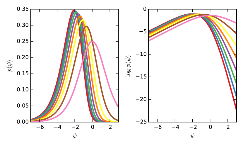
Figure 5: Density and log density of $p(\boldsymbol{\psi}\,|\,\boldsymbol{\alpha}=\boldsymbol{1})$, the density on $\boldsymbol{\psi}$ implied by a $K=9$ dimensional symmetric Dirichlet density on $\boldsymbol{\pi}$ with parameter $\alpha=1$.

Figure 6 shows the marginal densities on $\psi_{k}$ implied by a $K=9$ dimensional symmetric Dirichlet prior on $\boldsymbol{\pi}$ with $\alpha=1$. The densities of $\psi_{k}$ become increasingly skewed for small values of $k$, but they are still well approximate by a Gaussian distribution. In order to approximate a uniform distribution, we numerically compute the mean and variance of these densities to set the parameters of a diagonal Guassian distribution.

Appendix B Marginal Predictions with the Augmented Model

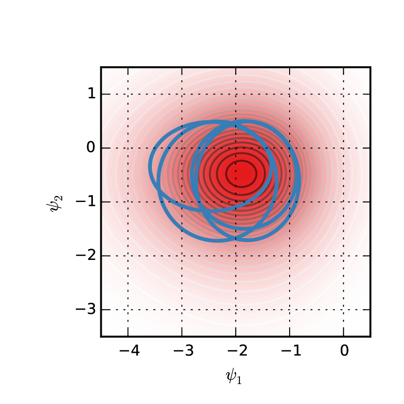
Figure 6: Marginal density, $p(\boldsymbol{\psi}\,|\,\boldsymbol{x})$ in red shading along with the ellipses of multivariate normal conditional distribution $p(\boldsymbol{\psi}\,|\,\boldsymbol{x},\boldsymbol{\omega})$ for 4 steps of the Gibbs sampler. In Gaussian models where we aim to predict $\boldsymbol{\psi}_{\mathsf{test}}$ on test data, there are substantial gains to be had from making marginal predictions of $\boldsymbol{\psi}_{\mathsf{test}}\,|\,\boldsymbol{x},\boldsymbol{\omega}$, integrating out $\boldsymbol{\psi}_{\mathsf{train}}$. The key is that the conditional densities overlap substantially with the marginal density.

One of the primary advantages offered by the Pólya-gamma augmentation is the ability to make marginal predictions about $\boldsymbol{\psi}_{\mathsf{test}}\,|\,\boldsymbol{x},\boldsymbol{\omega}$, integrating out the value of $\boldsymbol{\psi}_{\mathsf{train}}$. For example, in the GP multinomial regression models described in the main text, the methods were evaluated on the accuracy of their predictions about future name probabilities, which were functions of $\boldsymbol{\psi}_{\mathsf{test}}$. When $p(\boldsymbol{\psi}_{\mathsf{train}})$ and $p(\boldsymbol{\psi}_{\mathsf{test}}\,|\,\boldsymbol{\psi}_{\mathsf{train}})$ are both Gaussian, we can integrate out the latent training variables in order to predict their test values. In a latent Gaussian-multinomial model, the posterior distribution over those latent training variables is non-Gaussian, but after Pólya-gamma augmentation, it is rendered Gaussian.

With the augmentation, we can write

$$p(\boldsymbol{\psi}_{\mathsf{test}}\,|\,\boldsymbol{x}) \approx\frac{1}{M}\sum_{m=1}^{M}\int p(\boldsymbol{\psi}_{\mathsf{test}}\,|\,\boldsymbol{\psi}_{\mathsf{train}})\,p(\boldsymbol{\psi}_{\mathsf{train}}\,|\,\boldsymbol{x},\boldsymbol{\omega}^{(m)})\,\mathrm{d}\boldsymbol{\psi}_{\mathsf{train}} \boldsymbol{\omega}^{(m)} \sim p(\boldsymbol{\omega}\,|\,\boldsymbol{x}),$$

and perform Monte Carlo integration over $\boldsymbol{\omega}$ in order to compute the predictive distribution. By contrast, in the standard formulation we must perform Monte Carlo integration over $\boldsymbol{\psi}$,

$$p(\boldsymbol{\psi}_{\mathsf{test}}\,|\,\boldsymbol{x}) =\frac{1}{M}\sum_{m=1}^{M}p(\boldsymbol{\psi}_{\mathsf{test}}\,|\,\boldsymbol{\psi}_{\mathsf{train}}^{(m)}) \boldsymbol{\psi}_{\mathsf{train}}^{(m)} \sim p(\boldsymbol{\psi}_{\mathsf{train}}\,|\,\boldsymbol{x}).$$

Why does the augmented model confer a predictive advantage? It does not come from performing Monte Carlo integration over a smaller dimension since $\boldsymbol{\omega}$ and $\boldsymbol{\psi}_{\mathsf{train}}$ are of the same size. Instead, it comes from the ability of the conjugate Gibbs sampler to efficiently mix over $\boldsymbol{\psi}$ and $\boldsymbol{\omega}$, and from the ability of a single sample of $\boldsymbol{\omega}$ to render a conditional Gaussian distribution over $\boldsymbol{\psi}$ that captures much of the volume of the true marginal distribution.

This latter point is illustrated in Figure 6. The red shading shows the true marginal density of $\boldsymbol{\psi}$ and the blue ellipses show the conditional density for a fixed value of $\boldsymbol{\omega}$. Each ellipse capture a significant amount of the marginal distribution, indicating that with a single sample of $\boldsymbol{\omega}$ we can integrate over a substantial amount of the uncertainty in $\boldsymbol{\psi}$. This example is only for a $K=3$ dimensional multinomial observation, but this intuition should extend to higher dimensions in which the advantages of analytical integration should be more readily apparent.

Appendix C Variational Inference for Correlated Topic Models

We use the following factorized approximation to the posterior distribution,

$$p(\{\boldsymbol{\psi}_{d},\boldsymbol{\omega}_{d}\},\{\boldsymbol{\beta}_{t}\},\{\{z_{n,d}\}\},\boldsymbol{\mu}_{\theta},\boldsymbol{\Sigma}_{\theta},\boldsymbol{\mu}_{\beta},\boldsymbol{\Sigma}_{\beta}\,|\,\{\{w_{n,d}\}\})\\ \approx\left[\prod_{d=1}^{D}q(\boldsymbol{\psi}_{d})\prod_{t=1}^{T}q(\omega_{d,t})\prod_{n=1}^{N_{d}}q(z_{n,d})\right]\left[\prod_{t=1}^{T}q(\boldsymbol{\beta}_{t})\right]q(\boldsymbol{\mu}_{\theta},\boldsymbol{\Sigma}_{\theta}).$$

First let’s consider the variational distribution for $\boldsymbol{\psi}_{d}$ and $\boldsymbol{\omega}_{d}$. From the conjugacy of the model, we have

$$q(\boldsymbol{\psi}_{d}) =\mathcal{N}(\boldsymbol{\psi}_{d}\,|\,\widetilde{\boldsymbol{\mu}}_{\boldsymbol{\theta}_{d}},\widetilde{\boldsymbol{\Sigma}}_{\boldsymbol{\theta}_{d}})$$

$$\widetilde{\boldsymbol{\mu}}_{\boldsymbol{\theta}_{d}} =\widetilde{\boldsymbol{\Sigma}}_{\boldsymbol{\theta}_{d}}\left[\mathbb{E}[\boldsymbol{\kappa}(\boldsymbol{c}_{d},N_{d})]+\mathbb{E}[\boldsymbol{\Sigma}_{\theta}^{-1}\boldsymbol{\mu}_{\theta}]\right]^{-1}$$

$$\widetilde{\boldsymbol{\Sigma}}_{\boldsymbol{\theta}_{d}} =\left[\mathbb{E}[\text{diag}(\boldsymbol{\omega}_{d})]+\mathbb{E}[\boldsymbol{\Sigma}_{\boldsymbol{\theta}}^{-1}]\right]^{-1},$$

and

$$\mathbb{E}[(\boldsymbol{\kappa}(\boldsymbol{c}_{d},N_{d}))_{t}] =\mathbb{E}[c_{d,t}-N_{d,t}/2]$$

$$=\mathbb{E}[c_{d,t}-(N_{d}-\sum_{t^{\prime}<t}c_{d,t^{\prime}})/2]$$

$$=\mathbb{E}[c_{d,t}]+\frac{1}{2}\sum_{t^{\prime}<t}\mathbb{E}[c_{d,t^{\prime}}]-\frac{N_{d}}{2}$$

$$\mathbb{E}[c_{d,t}] =\sum_{n=1}^{N_{d}}\mathbb{E}[z_{n,d}=t].$$

The factor for $\boldsymbol{\omega}_{d}$ is not available in closed form. We have,

$$\log q(\boldsymbol{\omega}_{d}) =\mathbb{E}_{\boldsymbol{\psi}_{d},\boldsymbol{z}_{d}}[\log p(\boldsymbol{z}_{d}\,|\,\boldsymbol{\psi}_{d},\boldsymbol{\omega}_{d})]+\text{const.}$$

$$=\mathbb{E}_{\boldsymbol{\psi}_{d},\boldsymbol{z}_{d}}[\log\mathrm{PG}(\boldsymbol{\omega}_{d}\,|\,\boldsymbol{N}(\boldsymbol{c}_{d}),\boldsymbol{\psi}_{d})]+\text{const.}$$

Instead, following Zhou et al. [2012], we restrict the variational factor over $\omega$ to take the form of a Polya-gamma distribution,  ${\omega_{d,t}\sim\mathrm{PG}(\omega_{d,t}\,|\,N_{d,t},\psi_{d,t})}$, where ${N_{d,t}=[N(\boldsymbol{c}_{d})]_{t}}$. To perform the updates for $\boldsymbol{\psi}_{d}$, we only need the expectations of $\omega_{d,t}$ under the Pólya-gamma factors. The mean of $PG(b,c)$ distribution is available in closed form: $\mathbb{E}_{\omega\sim\mathrm{PG}(b,c)}[\omega]=\frac{b}{2c}\tanh(\frac{c}{2})$. Since the parameters of the Pólya-gamma distribution have variational factors, we use iterated expectations and Monte Carlo methods to approximate the expectation,

$$\mathbb{E}[q(\omega_{d,t})] =\mathbb{E}_{\boldsymbol{\psi}_{d,t},\boldsymbol{z}_{d}}\left[\mathbb{E}_{\boldsymbol{\omega}_{d,t}|\boldsymbol{\psi}_{d,t},\boldsymbol{z}_{d}}[\mathrm{PG}(\omega_{d,t}\,|\,\boldsymbol{N}(\boldsymbol{c}_{d})_{t},\boldsymbol{\psi}_{d,t})]\right]$$

$$=\frac{1}{2}\mathbb{E}_{\boldsymbol{z}_{d}}\left[\boldsymbol{N}(\boldsymbol{c}_{d})_{t}\right]\mathbb{E}_{\psi_{d,t}}\left[\frac{\tanh(\psi_{d,t}/2)}{\psi_{d,t}}\right]$$

$$=\frac{1}{2}\left(N_{d}-\sum_{t^{\prime}=1}^{t}\mathbb{E}_{\boldsymbol{z}_{d}}\left[c_{d,t^{\prime}}\right]\right)\mathbb{E}_{\psi_{d,t}}\left[\frac{\tanh(\psi_{d,t}/2)}{\psi_{d,t}}\right],$$

$$=\frac{1}{2}\left(N_{d}-\sum_{t^{\prime}=1}^{t-1}\sum_{n=1}^{N_{d}}\mathbb{E}_{\boldsymbol{z}_{d}}[z_{n,d}=t^{\prime}]\right)\mathbb{E}_{\psi_{d,t}}\left[\frac{\tanh(\psi_{d,t}/2)}{\psi_{d,t}}\right].$$

The updates for the global topic distribution parameters, $\boldsymbol{\mu}_{\theta}$ and $\boldsymbol{\Sigma}_{\theta}$, depend only on their normal inverse-Wishart prior and the expectations with respect to $q(\boldsymbol{\psi}_{d})$. These follow their standard form, see, for example, Bishop [2006].

The variational updates for $z_{n,d}$ and $\boldsymbol{\beta}_{t}$ are straightforward.

$$\log q(z_{n,d}) =\mathbb{E}_{\boldsymbol{\theta}_{d},\boldsymbol{\beta}}\left[\log p(w_{n,d}\,|\,z_{n,d},\boldsymbol{\theta}_{d},\{\boldsymbol{\beta}_{t}\})\right]+\text{ const.}$$

$$=\mathbb{E}_{\boldsymbol{\theta}_{d},\boldsymbol{\beta}}\left[\sum_{t=1}^{T}z_{n,d}(\log\beta_{t,w_{d,n}}+\log\theta_{d,t})\right]+\text{ const.}$$

$$=\sum_{t=1}^{T}z_{n,d}(\mathbb{E}_{\boldsymbol{\beta}}[\log\beta_{t,w_{n,d}}]+\mathbb{E}_{\boldsymbol{\theta}_{d}}[\log\theta_{d,t}])+\text{ const.}$$

This implies that $q(z_{n,d})$ is categorical with parameters,

$$q(z_{n,d}) =\mathrm{Cat}(z_{n,d}\,|\,\widetilde{\boldsymbol{u}}_{n,d}),$$

$$\widetilde{u}_{n,d,t} =\frac{1}{Z}\exp\left\{\mathbb{E}_{\boldsymbol{\beta}}[\log\beta_{t,w_{n,d}}]+\mathbb{E}_{\boldsymbol{\theta}_{d}}[\log\theta_{d,t}]\right\},$$

$$Z =\sum_{t^{\prime}=1}^{T}\exp\left\{\mathbb{E}_{\boldsymbol{\beta}}[\log\beta_{t^{\prime},w_{n,d}}]+\mathbb{E}_{\boldsymbol{\theta}_{d}}[\log\theta_{d,t^{\prime}}]\right\}$$

The challenge is that $\mathbb{E}_{\boldsymbol{\theta}_{d}}[\log\theta_{d,t}]$ is not available in closed form. Instead we must approximate it by Monte Carlo sampling the corresponding value of $\boldsymbol{\psi}_{d}$.

Last,

$$\log q(\boldsymbol{\beta}_{t}) =\mathbb{E}\left[\log p(\boldsymbol{w}\,|\,\boldsymbol{z},\boldsymbol{\theta})+\log p(\boldsymbol{\beta}_{t}\,|\,\boldsymbol{\alpha})\right]+\text{ const.}$$

$$=\sum_{d=1}^{D}\sum_{n=1}^{N_{d}}\mathbb{E}[z_{n,d}=t]\log\beta_{t,w_{n,d}}+\sum_{v=1}^{V}(\alpha_{v}-1)\log\beta_{t,v}+\text{ const.}$$

We recognize this as a Dirichlet distribution,

$$q(\boldsymbol{\beta}_{t}) =\mathrm{Dir}(\boldsymbol{\beta}_{t}\,|\,\widetilde{\boldsymbol{\alpha}}_{t}), \widetilde{\alpha}_{t,v} =\sum_{d=1}^{D}\sum_{n=1}^{N_{d}}\mathbb{I}[w_{n,d}=v]\mathbb{E}[z_{n,d}=t]+\alpha_{v}.$$

The data local variables, $z_{n,d}$, $\boldsymbol{\psi}_{d}$, and $\boldsymbol{\omega}_{d}$, are conditionally independent across documents. Moreover, since the model is fully conjugate, the expectations required to update the global variables, $\boldsymbol{\beta}_{t}$, $\boldsymbol{\mu}_{\theta}$, and $\boldsymbol{\Sigma}_{\theta}$ depend on sufficient statistics that are derived from summmations over documents. Rather than summing over the entire corpus of documents, we can get an unbiased estimate of the sufficient statistics by considering a random subset, or mini-batch, per iteration. This is the key to stochastic variational inference (SVI) algorithms Hoffman et al. [2013], which have been widely successful in scalable topic modeling applications. Those same gains in scalability are readily applicable in this correlated topic model formulation.

References

- Andrieu et al. (2010) Christophe Andrieu, Arnaud Doucet, and Roman Holenstein. Particle Markov chain Monte Carlo methods. Journal of the Royal Statistical Society: Series B (Statistical Methodology), 72(3):269–342, 2010.
- Murray et al. (2010) Iain Murray, Ryan P. Adams, and David J.C. MacKay. Elliptical slice sampling. Journal of Machine Learning Research: Workshop and Conference Proceedings (AISTATS), 9:541–548, 05/2010 2010. URL http://hips.seas.harvard.edu/files/w/papers/murray-adams-mackay-2010a.pdf.
- Polson et al. (2013) Nicholas G Polson, James G Scott, and Jesse Windle. Bayesian inference for logistic models using Pólya–gamma latent variables. Journal of the American Statistical Association, 108(504):1339–1349, 2013.
- Zhou et al. (2012) Mingyuan Zhou, Lingbo Li, David Dunson, and Lawrence Carin. Lognormal and gamma mixed negative binomial regression. In Proceedings of the International Conference on Machine Learning, volume 2012, page 1343, 2012.
- Ren et al. (2011) Lu Ren, Lan Du, Lawrence Carin, and David Dunson. Logistic stick-breaking process. The Journal of Machine Learning Research, 12:203–239, 2011.
- Khan et al. (2012) Mohammad E Khan, Shakir Mohamed, Benjamin M Marlin, and Kevin P Murphy. A stick-breaking likelihood for categorical data analysis with latent Gaussian models. In International Conference on Artificial Intelligence and Statistics, pages 610–618, 2012.
- Albert and Chib (1993) James H Albert and Siddhartha Chib. Bayesian analysis of binary and polychotomous response data. Journal of the American statistical Association, 88(422):669–679, 1993.
- Holmes et al. (2006) Chris C Holmes, Leonhard Held, et al. Bayesian auxiliary variable models for binary and multinomial regression. Bayesian Analysis, 1(1):145–168, 2006.
- Blei and Lafferty (2006a) David Blei and John Lafferty. Correlated topic models. Advances in Neural Information Processing Systems, 18:147, 2006a.
- Blei et al. (2003) David M Blei, Andrew Y Ng, and Michael I Jordan. Latent Dirichlet allocation. the Journal of machine Learning research, 3:993–1022, 2003.
- Chen et al. (2013) Jianfei Chen, Jun Zhu, Zi Wang, Xun Zheng, and Bo Zhang. Scalable inference for logistic-normal topic models. In Advances in Neural Information Processing Systems, pages 2445–2453, 2013.
- Blei and Lafferty (2006b) David M Blei and John D Lafferty. Dynamic topic models. In Proceedings of the International Conference on Machine Learning, pages 113–120. ACM, 2006b.
- Wang and Grimson (2008) Xiaogang Wang and Eric Grimson. Spatial latent Dirichlet allocation. In Advances in Neural Information Processing Systems, pages 1577–1584, 2008.
- Hoffman et al. (2013) Matthew D Hoffman, David M Blei, Chong Wang, and John Paisley. Stochastic variational inference. The Journal of Machine Learning Research, 14(1):1303–1347, 2013.
- Belanger and Kakade (2015) David Belanger and Sham Kakade. A linear dynamical system model for text. In Proceedings of the International Conference on Machine Learning, 2015.
- Collobert and Weston (2008) Ronan Collobert and Jason Weston. A unified architecture for natural language processing: Deep neural networks with multitask learning. In Proceedings of the International Conference on Machine Learning, pages 160–167. ACM, 2008.
- Belanger and Kakade (2014) David Belanger and Sham Kakade. Embedding word tokens using a linear dynamical system. In NIPS 2014 Modern ML+NLP Workshop, 2014.
- Wan and Van Der Merwe (2000) Eric A Wan and Rudolph Van Der Merwe. The unscented Kalman filter for nonlinear estimation. In Adaptive Systems for Signal Processing, Communications, and Control Symposium 2000. AS-SPCC. The IEEE 2000, pages 153–158. IEEE, 2000.
- Thrun et al. (2005) Sebastian Thrun, Wolfram Burgard, and Dieter Fox. Probabilistic robotics. MIT press, 2005.
- Lindsten et al. (2012) Fredrik Lindsten, Thomas Schön, and Michael I Jordan. Ancestor sampling for particle Gibbs. In Advances in Neural Information Processing Systems, pages 2591–2599, 2012.
- Bishop (2006) Christopher M Bishop. Pattern recognition and machine learning. Springer, 2006.