On Lipschitz solutions for some forward-backward parabolic equations

Abstract.

We investigate the existence and properties of Lipschitz solutions for some forward-backward parabolic equations in all dimensions. Our main approach to existence is motivated by reformulating such equations into partial differential inclusions and relies on a Baire’s category method. In this way, the existence of infinitely many Lipschitz solutions to certain initial-boundary value problem of those equations is guaranteed under a pivotal density condition. Finally, we study two important cases of forward-backward anisotropic diffusion in which the density condition can be realized and therefore the existence results follow together with micro-oscillatory behavior of solutions. The first case is a generalization of the Perona-Malik model in image processing and the other that of Höllig’s model related to the Clausius-Duhem inequality in the second law of thermodynamics.

1. Introduction

The evolution process of many quantities in applications can be modeled by a diffusion partial differential equation of the form

(1.1) $$u_{t}=\operatorname{div}(A(Du))\quad\mbox{in $\Omega\times(0,T)$,}$$

where $\Omega\subset\mathbb{R}^{n}$ is a bounded domain, $T>0$ is any fixed number, and $u=u(x,t)$ is the density of the quantity at position $x$ and time $t$, with $Du=(u_{x_{1}},\cdots,u_{x_{n}})$ and $u_{t}$ denoting its spatial gradient and rate of change, respectively. The vector function $A\colon\mathbb{R}^{n}\to\mathbb{R}^{n}$ here represents the diffusion flux of the evolution process. The usual heat equation corresponds to the case of isotropic diffusion given by the Fourier law: $A(p)=kp\;(p\in\mathbb{R}^{n})$, where $k>0$ is the diffusion constant.

For standard diffusion equations, the flux $A(p)$ is assumed to be monotone; namely,

$$(A(p)-A(q))\cdot(p-q)\geq 0\quad(p,\,q\in\mathbb{R}^{n}).$$

In this case, equation (1.1) is parabolic and can be studied by the standard methods of parabolic equations and monotone operators [6, 29, 30]. In particular, when $A(p)$ is given by a smooth convex function $W(p)$ through $A(p)=D_{p}W(p)\;(p\in\mathbb{R}^{n}),$ (1.1) can be viewed and thus studied as a certain gradient flow generated by the energy functional

$$I(u)=\int_{\Omega}W(Du(x))\,dx.$$

However, for certain applications of the evolution process to some important physical problems, the underlying diffusion fluxes $A(p)$ may not be monotone, yielding non-parabolic equations (1.1). In this paper, we study the diffusion equation (1.1) for some non-monotone diffusion fluxes $A(p).$ We focus on the initial-boundary value problem

(1.2) $$\begin{cases}u_{t}=\operatorname{div}(A(Du))&\mbox{in $\Omega_{T}$,}\\ A(Du)\cdot\mathbf{n}=0&\mbox{on $\partial\Omega\times(0,T)$,}\\ u=u_{0}&\mbox{on $\Omega\times\{t=0\},$}\end{cases}$$

where $\Omega_{T}=\Omega\times(0,T)$, $\mathbf{n}$ is the outer unit normal on $\partial\Omega$, $u_{0}=u_{0}(x)$ is a given initial datum, and the flux $A(p)$ is of the form

(1.3) $$A(p)=f(|p|^{2})p\quad(p\in\mathbb{R}^{n}),$$

given by a function $f\colon[0,\infty)\to\mathbb{R}$ with profile $\sigma(s)=sf(s^{2})$ having one of the graphs in Figures 1, 2 and 3 below. (Precise structural assumptions on $\sigma(s)=sf(s^{2})$ will be given in Section 3.)

Figure 1. Case I: Perona-Malik type of profiles $\sigma(s)$.

Figure 2. Case II: Höllig type of profiles $\sigma(s)$ with $\sigma(s_{2})>0$.

Figure 3. Case II: Höllig type of profiles $\sigma(s)$ with $\sigma(s_{2})=0$.

The two cases in Figures 1, 2 and 3 correspond to the applications in image processing proposed by Perona and Malik [35] and in phase transitions of thermodynamics studied by Höllig [21]. For these diffusions, we have

$$\sigma^{\prime}(\sqrt{s})=f(s)+2sf^{\prime}(s)<0\quad\mbox{for some range of $s>0$.}$$

In these cases, the diffusion is anisotropic since the diffusion matrix $(A^{i}_{p_{j}})$, where

$$A_{p_{j}}^{i}(p)=f(|p|^{2})\delta_{ij}+2f^{\prime}(|p|^{2})p_{i}p_{j}\quad(i,\,j=1,2,\cdots,n),$$

has the eigenvalues $f(|p|^{2})$ (of multiplicity $n-1$) and $f(|p|^{2})+2|p|^{2}f^{\prime}(|p|^{2});$ hence the diffusion coefficients could also be negative, and problem (1.2) becomes forward-backward parabolic. Moreover, setting

$$W(p)=\int_{0}^{|p|}\sigma(r)\,dr,\quad I(u)=\int_{\Omega}W(Du)\,dx,$$

the initial-boundary value problem (1.2) becomes a $L^{2}$-gradient flow of the energy functional $I(u);$ however, $I(u)$ is non-convex. Consequently, neither the standard methods of parabolic equations and monotone operators nor the non-linear semigroup theory can be applied to study (1.2).

Forward-backward parabolic equations have found many important applications in the mathematical modeling of some physical problems, but mathematically, due to the backward parabolicity, the initial-boundary value problem (1.2) of such equations is highly ill-posed, and in many cases even the notion and existence of reasonable solutions remain largely unsettled.

In [35], the original Perona-Malik model (1.2) in image processing used the profile

(1.4) $$\sigma(s)=se^{-s^{2}/2s_{0}^{2}}\quad\mbox{or}\quad\sigma(s)=\frac{s}{1+{s^{2}}/{s_{0}^{2}}}$$

for denoising and edge enhancement of a computer vision; in this case, we call (1.1) the Perona-Malik equation. In this model, $u(x,t)$ represents an improved version of the initial gray level $u_{0}(x)$ of a noisy picture. The anisotropic diffusion $\operatorname{div}(A(Du))$ is forward parabolic in the subcritical region where $|Du|<s_{0}$ and backward parabolic in the supercritical region where $|Du|>s_{0}.$ The expectation of the model is that disturbances with small gradient in the subcritical region will be smoothed out by the forward parabolic diffusion, while sharp edges corresponding to large gradient in the supercritical region will be enhanced by the backward parabolic equation. Such expected phenomenology has been implemented and observed in some numerical experiments [15, 35], showing the stability and effectiveness of the model. Mathematically, there have been extensive works on the Perona-Malik type of equations with profiles $\sigma(s)$ as in Figure 1; however, most of these works have focused on the analysis of numerical or approximate solutions by different methods. For example, in dimension $n=1$, the singular perturbation and its $\Gamma$-limit related to the Perona-Malik type of equations were investigated in [3, 4]. In [20], a mild regularization of the Perona-Malik equation with a viscous term was used to extract a unique approximate Young measure solution in any dimension. The works [8, 39] studied Young measure solutions for the Perona-Malik equation in dimensions $n=1$ and $n=2$. Also the works [15, 16] focused on the numerical schemes for the Perona-Malik model. Recently, classical solutions for the Perona-Malik equation were studied in [17, 18], where the existence of solutions was proved for certain initial data $u_{0}$ that can be transcritical in the sense that the sets $\{|Du_{0}(x)|>s_{0}\}$ and $\{|Du_{0}(x)|<s_{0}\}$ are both nonempty ($s_{0}$ is the number in Figure 1); however, their initial data cannot be arbitrarily prescribed.

For the Höllig model, the one-dimensional forward-backward parabolic problem (1.2) under the piecewise linearity assumption on the profile $\sigma(s)$ (see Figure 4) was studied in [21], motivated by the Clausius-Duhem inequality in the second law of thermodynamics in continuum mechanics. For such a special profile, it was proved that there exist infinitely many $L^{2}$-weak solutions to (1.2) in dimension $n=1$. The piecewise linearity of $\sigma(s)$ in $n=1$ was much relaxed later to include a more general class of profiles $\sigma(s)$ (as in Figure 2) in the work of Zhang [44], using an entirely different approach from Höllig’s.

Figure 4. Höllig’s piecewise linear profile $\sigma(s)$.

The question concerning the existence of exact weak solutions to problem (1.2) of the Perona-Malik and Höllig types had remained open until Zhang [43, 44] first established that the one-dimensional problem (1.2) of each type has infinitely many Lipschitz solutions for any suitably given smooth initial data $u_{0}.$ Zhang’s pivotal idea was to reformulate equation (1.1) in $n=1$ into a $2\times 2$ non-homogeneous partial differential inclusion and then to prove the existence by using a modified method of convex integration, following the ideas of [28, 32]. The study of general partial differential inclusions has stemmed from the successful understanding of homogeneous differential inclusions of the form $Du(x)\in K$, first encountered in the study of crystal microstructures [2, 9, 32]; recently, the methods of differential inclusions have been successfully applied to other important problems; see, e.g., [10, 14, 31, 33, 38, 41].

In general, a function $u\in W^{1,\infty}(\Omega_{T})$ is called a Lipschitz solution to problem (1.2) provided that equality

(1.5) $$\int_{\Omega}(u(x,s)\zeta(x,s)-u_{0}(x)\zeta(x,0))dx=\int_{0}^{s}\int_{\Omega}(u\zeta_{t}-A(Du)\cdot D\zeta)dxdt$$

holds for each $\zeta\in C^{\infty}(\bar{\Omega}_{T})$ and each $s\in[0,T].$ Let $\zeta\equiv 1$; then it is immediate from the definition that any Lipschitz solution $u$ to (1.2) conserves the total mass over time:

$$\int_{\Omega}u(x,t)dx=\int_{\Omega}u_{0}(x)dx\quad\forall t\in[0,T].$$

In [26], we extended Zhang’s method of partial differential inclusions to the Perona-Malik type of equations in all dimensions $n$ for balls $\Omega=B_{R}(0):=\{x\in\mathbb{R}^{n}\,|\,|x|<R\}$ and non-constant radially symmetric smooth initial data $u_{0}.$ In this case, the $n$-dimensional equation for radial solutions can still be reformulated into a $2\times 2$ non-homogeneous partial differential inclusion, and the existence of infinitely many radial Lipschitz solutions to (1.2) is established. However, for general domains and initial data, the $n$-dimensional problem (1.2) can only be recast as a $(1+n)\times(n+1)$ non-homogeneous partial differential inclusion that has some uncontrollable gradient components, making the construction of Lipschitz solutions for this inclusion impractical. In our recent work [27], we overcame this difficulty by developing a suitably modified density method, still motivated by the method of differential inclusions but based on a Baire’s category argument. In this work, it was proved that for all bounded convex domains $\Omega\subset\mathbb{R}^{n}$ with $\partial\Omega\in C^{2+\alpha}$ and initial data $u_{0}\in C^{2+\alpha}(\bar{\Omega})$ with $Du_{0}\cdot\mathbf{n}=0$ on $\partial\Omega$, there exist infinitely many Lipschitz solutions to (1.2) for the exact Perona-Malik diffusion flux $A(p)=\frac{p}{1+|p|^{2}}$ ($p\in\mathbb{R}^{n}$). However, the proof heavily relies on the explicit formula of the rank-one convex hull of a certain matrix set defined by this special flux; such an explicit formula for the general Perona-Malik type of flux $A(p)$ (with profile $\sigma(s)$ as in Figure 1) is unattainable.

The main purpose of this paper is to generalize the method of [27] to problem (1.2) in all dimensions for general diffusion profiles of the Perona-Malik and Höllig types. To state our main theorems, we make the following assumptions on the domain $\Omega$ and initial datum $u_{0}$:

(1.6) $$\begin{cases}\mbox{$\Omega\subset\mathbb{R}^{n}$ is a bounded domain with $\partial\Omega$ of $C^{2+\alpha}$,}\\ \mbox{$u_{0}\in C^{2+\alpha}(\bar{\Omega})$ is non-constant with $Du_{0}\cdot\mathbf{n}|_{\partial\Omega}=0,$}\end{cases}$$

where $\alpha\in(0,1)$ is a given number. Without specifying the precise conditions on the profiles $\sigma(s)$ for Cases I and II, we first state our main existence theorems as below.

Theorem 1.1.

Assume condition $(\ref{assume-1})$ is fulfilled. Let $A(p)$ be given by $(\ref{fun-A})$ with the profile $\sigma(s).$ Then problem $(\ref{ib-P})$ has infinitely many Lipschitz solutions in the following two cases.

Case I: $\sigma(s)$ is of the Perona-Malik type as in Figure 1, and in addition $\Omega$ is convex.

Case II: $\sigma(s)$ is of the Höllig type as in Figure 2, and in addition $u_{0}$ satisfies $|Du_{0}(x_{0})|\in(s_{1}^{*},s_{2}^{*})$ at some $x_{0}\in\Omega.$

The precise assumptions on the profiles $\sigma(s)$ and detailed statements of the theorems for both cases will be given later (see Theorems 3.1 and 3.5) along with some discussions about a certain implication of our result on the Perona-Malik model in image processing and the breakdown of uniqueness for the Höllig type of equations.

In certain cases, among infinitely many Lipschitz solutions, problem (1.2) admits a unique classical solution; we have the following result (see also [24]).

Theorem 1.2.

Assume condition $(\ref{assume-1})$ is fulfilled and $\Omega$ is convex. Let $A(p)$ be given by $(\ref{fun-A})$ with the profile $\sigma(s).$ Assume $\|Du_{0}\|_{L^{\infty}(\Omega)}<s_{0}$ if $\sigma(s)$ is of the Perona-Malik type or $\|Du_{0}\|_{L^{\infty}(\Omega)}<s_{1}$ if $\sigma(s)$ is of the Höllig type. Then problem $(\ref{ib-P})$ has a unique solution $u\in C^{2+\alpha,1+\alpha/2}(\bar{\Omega}_{T})$ satisfying $\|Du\|_{L^{\infty}(\Omega_{T})}=\|Du_{0}\|_{L^{\infty}(\Omega)}.$

This theorem will be also separated into Cases I and II in Section 3 in order to be compared with our detailed main results, Theorems 3.1 and 3.5.

Finally, we have the following coexistence result.

Theorem 1.3.

Assume that $\Omega=B_{R}(0)$ is a ball in $\mathbb{R}^{n}$ and that $u_{0}$ is radial and satisfies condition $(\ref{assume-1})$. Then there are infinitely many radial and non-radial Lipschitz solutions to (1.2).

The rest of the paper is organized as follows. Section 2 begins with a motivational approach to problem (1.2) as a non-homogeneous partial differential inclusion and its limitation. Then the general existence theorem, Theorem 2.2, is formulated under a key density hypothesis, and some general properties of Lipschitz solutions to (1.2) are also provided. In section 3, precise structural conditions on the profiles $\sigma(s)$ of the Perona-Malik and Höllig types are specified, and the detailed statements for the main result, Theorem 1.1, are introduced as Theorems 3.1 and 3.5 that are followed by some remarks and related results. Section 4 prepares some useful results that may be of independent interest. As the core analysis of the paper, the geometry of related matrix sets is scrutinized in Section 5, leading to the relaxation result on a homogeneous differential inclusion, Theorem 5.8. Section 6 is devoted to the construction of suitable boundary functions and admissible sets for Cases I and II in the contexts of Theorems 3.1 and 3.5, respectively. Then the pivotal density hypothesis in each case is realized in Section 7, completing the proofs of Theorems 3.1 and 3.5. Lastly, Section 8 deals with the proof of the coexistence result, Theorem 1.3.

Throughout the paper, we use the boldface letters for Cases I and II for clear distinction. The paper follows a parallel exposition to deal with both cases simultaneously. But for a better readability, we strongly recommend for a reader to follow each case one at a time.

2. Existence by a general density approach

Here and below, we assume without loss of generality that the initial datum $u_{0}\in W^{1,\infty}(\Omega)$ in problem (1.2) satisfies

(2.1) $$\int_{\Omega}u_{0}(x)\,dx=0,$$

since otherwise we may solve (1.2) with initial datum $\tilde{u}_{0}=u_{0}-\bar{u}_{0},$ where $\bar{u}_{0}=\frac{1}{|\Omega|}\int_{\Omega}u_{0}\,dx$.

2.1. Motivation: non-homogeneous partial differential inclusion

To motivate our approach, let us reformulate problem (1.2) into a non-homogeneous partial differential inclusion.

First, assume that we have a function $\Phi=(u^{*},v^{*})\in W^{1,\infty}(\Omega_{T};\mathbb{R}^{1+n})$ satisfying

(2.2) $$\begin{cases}u^{*}(x,0)=u_{0}(x),&x\in\Omega,\\ \operatorname{div}v^{*}(x,t)=u^{*}(x,t),&\mbox{a.e. $(x,t)\in\Omega_{T}$},\\ v^{*}(\cdot,t)\cdot\mathbf{n}|_{\partial\Omega}=0,&t\in[0,T],\end{cases}$$

which will be called a boundary function for the initial datum $u_{0}.$

Let $A\in C(\mathbb{R}^{n};\mathbb{R}^{n})$ be the diffusion flux. For each $l\in\mathbb{R}$, let $K(l)$ be a subset of the matrix space $\mathbb{M}^{(1+n)\times(n+1)}$ defined by

(2.3) $$K(l)=\left\{\begin{pmatrix}p&c\\ B&A(p)\end{pmatrix}\,\Big{|}\,p\in\mathbb{R}^{n},\,c\in\mathbb{R},\,B\in\mathbb{M}^{n\times n},\,\operatorname{tr}B=l\right\}.$$

Suppose that a function $w=(u,v)\in W^{1,\infty}(\Omega_{T};\mathbb{R}^{1+n})$ solves the Dirichlet problem of non-homogeneous partial differential inclusion

(2.4) $$\begin{cases}\nabla w(x,t)\in K(u(x,t)),&\textrm{a.e. $(x,t)\in\Omega_{T}$,}\\ w(x,t)=\Phi(x,t),&(x,t)\in\partial\Omega_{T},\end{cases}$$

where $\nabla w$ is the space-time Jacobian matrix of $w$:

$$\nabla w=\begin{pmatrix}Du&u_{t}\\ Dv&v_{t}\end{pmatrix}.$$

Then it can be easily shown that $u$ is a Lipschitz solution to $(\ref{ib-P})$.

Although solving problem (2.4) is sufficient to obtain a Lipschitz solution to (1.2), all known general existence results [12, 34] are not applicable to solve (2.4). If $n=1$, (2.4) implies $v_{x}=u$ and thus $v\in W^{1,\infty}$ if $u\in W^{1,\infty}$; so Zhang [43, 44] was able to solve (2.4) for the Perona-Malik and Höllig types in dimension $n=1$ by using a modified convex integration method. However, for $n\geq 2$, since it is impossible to bound $\|Dv\|_{L^{\infty}(\Omega_{T})}$ in terms of $\operatorname{div}v$, the function $v$ may not be in $W^{1,\infty}(\Omega_{T};\mathbb{R}^{n})$ even when $u\in W^{1,\infty}(\Omega_{T});$ therefore, solving (2.4) in $W^{1,\infty}(\Omega_{T};\mathbb{R}^{1+n})$ is impractical in dimensions $n\geq 2$. To overcome this difficulty, we make the following key observation.

Proposition 2.1.

Suppose $u\in W^{1,\infty}(\Omega_{T})$ is such that $u(x,0)=u_{0}(x),$ there exists a vector function $v\in W^{1,2}((0,T);L^{2}(\Omega;\mathbb{R}^{n}))$ with weak time-derivative $v_{t}$ satisfying

(2.5) $$v_{t}=A(Du)\quad\mbox{a.e.\, in $\Omega_{T}$,}$$

and for each $\zeta\in C^{\infty}(\bar{\Omega}_{T})$ and each $t\in[0,T],$

(2.6) $$\int_{\Omega}v(x,t)\cdot D\zeta(x,t)\,dx=-\int_{\Omega}u(x,t)\zeta(x,t)\,dx.$$

Then $u$ is a Lipschitz solution to $(\ref{ib-P})$.

Proof.

To verify (1.5), given any $\zeta\in C^{\infty}(\bar{\Omega}_{T})$, let

$$g(t)=\int_{\Omega}u(x,t)\zeta(x,t)dx,\;\;h(t)=\int_{\Omega}u(x,t)\zeta_{t}(x,t)dx\quad(t\in[0,T]).$$

Then by (2.6), for each $\psi\in C^{\infty}_{c}(0,T),$

$$\int_{0}^{T}\psi_{t}gdt=-\int_{0}^{T}\int_{\Omega}\psi_{t}v\cdot D\zeta dxdt,\;\;\int_{0}^{T}\psi hdt=-\int_{0}^{T}\int_{\Omega}\psi v\cdot D\zeta_{t}dxdt.$$

Since $v\in W^{1,2}((0,T);L^{2}(\Omega;\mathbb{R}^{n}))$ and $v_{t}=A(Du)$ a.e. in $\Omega_{T}$, we have

$$\int_{0}^{T}\int_{\Omega}(\psi D\zeta)_{t}\cdot vdxdt=-\int_{0}^{T}\int_{\Omega}A(Du)\cdot\psi D\zeta\,dxdt.$$

As $(\psi D\zeta)_{t}=\psi_{t}D\zeta+\psi D\zeta_{t}$, combining the previous equations, we obtain

$$\int_{0}^{T}\psi_{t}g\,dt=\int_{0}^{T}\psi\left(-h+\int_{\Omega}A(Du)\cdot D\zeta\,dx\right)dt,$$

which proves that $g$ is weakly differentiable in $(0,T)$ with its weak derivative

$$g^{\prime}(t)=h(t)-\int_{\Omega}A(Du(x,t))\cdot D\zeta(x,t)\,dx\;\;\mbox{ a.e. $t\in(0,T)$.}$$

From this, upon integration, (1.5) follows for each $s\in[0,T].$ ∎

2.2. Admissible set and the density approach

Let $\Phi=(u^{*},v^{*})$ be any boundary function for $u_{0}$ defined by (2.2) above. Denote by $W^{1,\infty}_{u^{*}}(\Omega_{T})$, $W^{1,\infty}_{v^{*}}(\Omega_{T};\mathbb{R}^{n})$ the usual Dirichlet classes with boundary traces $u^{*},\,v^{*},$ respectively.

We say that $\mathcal{U}\subset W^{1,\infty}_{u^{*}}(\Omega_{T})$ is an admissible set provided that it is nonempty and bounded in $W^{1,\infty}_{u^{*}}(\Omega_{T})$ and that for each $u\in\mathcal{U}$, there exists a vector function $v\in W_{v^{*}}^{1,\infty}(\Omega_{T};\mathbb{R}^{n})$ satisfying

$$\operatorname{div}v=u \Omega_{T} \|v_{t}\|_{L^{\infty}(\Omega_{T})}\leq R$$   a.e. in , ,

where $R>0$ is any fixed number. If  $\mathcal{U}$ is an admissible set, for each $\epsilon>0$, let $\mathcal{U}_{\epsilon}$ be the set of all $u\in\mathcal{U}$ such that there exists a function $v\in W_{v^{*}}^{1,\infty}(\Omega_{T};\mathbb{R}^{n})$ satisfying

$$\begin{split}&\mbox{$\operatorname{div}v=u$ \, a.e. in $\Omega_{T}$,\quad$\|v_{t}\|_{L^{\infty}(\Omega_{T})}\leq R$,}\\ &\int_{\Omega_{T}}|v_{t}(x,t)-A(Du(x,t))|\,dxdt\leq\epsilon|\Omega_{T}|.\end{split}$$

The following general existence theorem relies on a pivotal density hypothesis of  $\mathcal{U}_{\epsilon}$ in $\mathcal{U}.$

Theorem 2.2.

Let  $\mathcal{U}\subset W^{1,\infty}_{u^{*}}(\Omega_{T})$ be an admissible set satisfying the density property:

(2.7) $$\mathcal{U}_{\epsilon} \mathcal{U} L^{\infty} \epsilon>0$$ is dense in under the -norm for each .

Then, given any $\varphi\in\mathcal{U}$, for each $\delta>0,$ there exists a Lipschitz solution $u\in W_{u^{*}}^{1,\infty}(\Omega_{T})$ to $(\ref{ib-P})$ satisfying $\|u-\varphi\|_{L^{\infty}(\Omega_{T})}<\delta.$ Furthermore, if $\mathcal{U}$ contains a function which is not a Lipschitz solution to $(\ref{ib-P}),$ then $(\ref{ib-P})$ itself admits infinitely many Lipschitz solutions.

Proof.

For clarity, we divide the proof into several steps.

1. Let $\mathcal{X}$ be the closure of  $\mathcal{U}$ in the metric space $L^{\infty}(\Omega_{T}).$ Then $(\mathcal{X},L^{\infty})$ is a nonempty complete metric space. By assumption, each $\mathcal{U}_{\epsilon}$ is dense in $\mathcal{X}.$ Moreover, since $\mathcal{U}$ is bounded in $W_{u^{*}}^{1,\infty}(\Omega_{T})$, we have $\mathcal{X}\subset W_{u^{*}}^{1,\infty}(\Omega_{T})$.

2. Let $\mathcal{Y}=L^{1}(\Omega_{T};\mathbb{R}^{n})$. For $h>0$, define $T_{h}\colon\mathcal{X}\to\mathcal{Y}$ as follows. Given any $u\in\mathcal{X}$, write $u=u^{*}+w$ with $w\in W_{0}^{1,\infty}(\Omega_{T})$ and define

$$T_{h}(u)=Du^{*}+D(\rho_{h}*w),$$

where $\rho_{h}(z)=h^{-N}\rho(z/h)$, with $z=(x,t)$ and $N=n+1$, is the standard $h$-mollifier in $\mathbb{R}^{N}$, and $\rho_{h}*w$ is the usual convolution in $\mathbb{R}^{N}$ with $w$ extended to be zero outside $\bar{\Omega}_{T}.$ Then, for each $h>0$, the map $T_{h}\colon(\mathcal{X},L^{\infty})\to(\mathcal{Y},L^{1})$ is continuous, and for each $u\in\mathcal{X}$,

$$\lim_{h\to 0^{+}}\|T_{h}(u)-Du\|_{L^{1}(\Omega_{T})}=\lim_{h\to 0^{+}}\|\rho_{h}*Dw-Dw\|_{L^{1}(\Omega_{T})}=0.$$

Therefore, the spatial gradient operator $D\colon\mathcal{X}\to\mathcal{Y}$ is the pointwise limit of a sequence of continuous maps $T_{h}\colon\mathcal{X}\to\mathcal{Y}$; hence $D\colon\mathcal{X}\to\mathcal{Y}$ is a Baire-one map. By Baire’s category theorem (e.g., [7, Theorem 10.13]), there exists a residual set $\mathcal{G}\subset\mathcal{X}$ such that the operator $D$ is continuous at each point of $\mathcal{G}.$ Since $\mathcal{X}\setminus\mathcal{G}$ is of the first category, the set $\mathcal{G}$ is dense in $\mathcal{X}$. Therefore, given any $\varphi\in\mathcal{X},$ for each $\delta>0$, there exists a function $u\in\mathcal{G}$ such that $\|u-\varphi\|_{L^{\infty}(\Omega_{T})}<\delta.$

3. We now prove that each $u\in\mathcal{G}$ is a Lipschitz solution to (1.2). Let $u\in\mathcal{G}$ be given. By the density of $\mathcal{U}_{\epsilon}$ in $(\mathcal{X},L^{\infty})$ for each $\epsilon>0$, for every $j\in\mathbb{N}$, there exists a function $u_{j}\in\mathcal{U}_{1/j}$ such that $\|u_{j}-u\|_{L^{\infty}(\Omega_{T})}<1/j$. Since the operator $D\colon(\mathcal{X},L^{\infty})\to(\mathcal{Y},L^{1})$ is continuous at $u$, we have $Du_{j}\to Du$ in $L^{1}(\Omega_{T};\mathbb{R}^{n}).$ Furthermore, from (2.2) and the definition of  $\mathcal{U}_{1/j}$, there exists a function $v_{j}\in W^{1,\infty}_{v^{*}}(\Omega_{T};\mathbb{R}^{n})$ such that for each $\zeta\in C^{\infty}(\bar{\Omega}_{T})$ and each $t\in[0,T],$

(2.8) $$\begin{split}&\int_{\Omega}v_{j}(x,t)\cdot D\zeta(x,t)\,dx=-\int_{\Omega}u_{j}(x,t)\zeta(x,t)\,dx,\\ \|(&v_{j})_{t}\|_{L^{\infty}(\Omega_{T})}\leq R,\quad\int_{\Omega_{T}}|(v_{j})_{t}-A(Du_{j})|\,dxdt\leq\frac{1}{j}|\Omega_{T}|.\end{split}$$

Since $v_{j}(x,0)=v^{*}(x,0)\in W^{1,\infty}(\Omega;\mathbb{R}^{n})$ and $\|(v_{j})_{t}\|_{L^{\infty}(\Omega_{T})}\leq R$, it follows that both sequences $\{v_{j}\}$ and $\{(v_{j})_{t}\}$ are bounded in $L^{2}(\Omega_{T};\mathbb{R}^{n})\approx L^{2}((0,T);L^{2}(\Omega;\mathbb{R}^{n})).$ So we may assume

$$v_{j}\rightharpoonup v (v_{j})_{t}\rightharpoonup v_{t} L^{2}((0,T);L^{2}(\Omega;\mathbb{R}^{n}))$$ and in

for some $v\in W^{1,2}((0,T);L^{2}(\Omega;\mathbb{R}^{n})),$ where $\rightharpoonup$ denotes the weak convergence. Upon taking the limit as $j\to\infty$ in (2.8), since $v\in C([0,T];L^{2}(\Omega;\mathbb{R}^{n}))$ and $A\in C(\mathbb{R}^{n};\mathbb{R}^{n})$, we obtain

$$\begin{split}\int_{\Omega}v(x,t)&\cdot D\zeta(x,t)\,dx=-\int_{\Omega}u(x,t)\zeta(x,t)\,dx\quad(t\in[0,T]),\\ &v_{t}(x,t)=A(Du(x,t))\quad a.e.\;(x,t)\in\Omega_{T}.\end{split}$$

Consequently, by Proposition 2.1, $u$ is a Lipschitz solution to (1.2).

4. Finally, assume $\mathcal{U}$ contains a function which is not a Lipschitz solution to (1.2); hence $\mathcal{G}\neq\mathcal{U}.$ Then $\mathcal{G}$ cannot be a finite set, since otherwise the $L^{\infty}$-closure $\mathcal{X}=\overline{\mathcal{G}}=\overline{\mathcal{U}}$ would be a finite set, making $\mathcal{U}=\mathcal{G}.$ Therefore, in this case, (1.2) admits infinitely many Lipschitz solutions. The proof is complete. ∎

The following result implies that the density approach streamlined in Theorem 2.2 can be useful only when problem (1.2) is non-parabolic, that is, when $A(p)$ is non-monotone.

Proposition 2.3.

If $A\colon\mathbb{R}^{n}\to\mathbb{R}^{n}$ is monotone, then $(\ref{ib-P})$ can have at most one Lipschitz solution.

Proof.

Let $u,\,\tilde{u}\in W^{1,\infty}(\Omega_{T})$ be any two Lipschitz solutions to (1.2). Use the identity (1.5) for both $u$ and $\tilde{u}$, subtract the two equations, take $\zeta=u-\tilde{u}$ (by approximations), and then apply the monotonicity of $A(p)$:

$$(A(Du)-A(D\tilde{u}))\cdot(Du-D\tilde{u})\geq 0$$

to obtain

$$\int_{\Omega}(u(x,s)-\tilde{u}(x,s))^{2}dx\leq\int_{0}^{s}\int_{\Omega}(u-\tilde{u})(u-\tilde{u})_{t}\,dxdt$$

$$=\frac{1}{2}\int_{\Omega}(u(x,s)-\tilde{u}(x,s))^{2}dx\quad(0\leq s\leq T).$$

Thus $u\equiv\tilde{u}$ in $\Omega_{T}.$ ∎

As a general property for Lipschitz solutions to (1.2) for all continuous fluxes $A(p)$ satisfying a positivity condition below, we prove the following result; clearly, the positivity condition is satisfied by the fluxes $A(p)$ given by (1.3) with the profiles $\sigma(s)$ of the Perona-Malik and Höllig types illustrated in Figures 1, 2 and 3. Note that the positivity condition is consistent with the Clausius-Duhem inequality in the second law of thermodynamics (e.g., [13, p. 79] and [40, p. 116]).

Proposition 2.4.

Let $u_{0}\in W^{1,\infty}(\Omega)$ and $A\colon\mathbb{R}^{n}\to\mathbb{R}^{n}$ satisfy the positivity condition:

$$A(p)\cdot p\geq 0\;\;(p\in\mathbb{R}^{n}).$$

Then any Lipschitz solution $u$ to $(\ref{ib-P})$ satisfies

(2.9) $$\min_{\bar{\Omega}}u_{0}\leq u\leq\max_{\bar{\Omega}}u_{0}\;\;\;\mbox{in $\Omega_{T}.$}$$

Proof.

Let $u\in W^{1,\infty}(\Omega_{T})$ be any Lipschitz solution to (1.2). By (1.5), for all $\zeta\in C^{\infty}(\bar{\Omega}_{T})$,

$$\int_{\Omega_{T}}u_{t}(x,t)\zeta(x,t)dxdt=-\int_{\Omega_{T}}A(Du)\cdot D\zeta dxdt;$$

hence by approximation, this equality holds for all $\zeta\in W^{1,\infty}(\Omega_{T}).$ Taking $\zeta(x,t)=\phi(x,t)\psi(t)$ with arbitrary $\phi\in W^{1,\infty}(\Omega_{T})$ and $\psi\in W^{1,\infty}(0,T)$, we deduce that

$$\int_{\Omega}u_{t}(x,t)\phi(x,t)\,dx=-\int_{\Omega}A(Du(x,t))\cdot D\phi(x,t)\,dx$$

for a.e. $t\in(0,T)$ and all $\phi\in W^{1,\infty}(\Omega_{T})$. Now taking $\phi=u^{2k-1}$ with $k=1,2,\cdots$, we have for a.e. $t\in(0,T),$

$$\begin{split}\frac{d}{dt}\Big{(}&\int_{\Omega}u^{2k}dx\Big{)}=2k\int_{\Omega}u_{t}\phi\,dx=-2k\int_{\Omega}A(Du)\cdot D\phi dx\\ &=-2k(2k-1)\int_{\Omega}u^{2k-2}A(Du)\cdot Dudx\leq 0.\end{split}$$

From this we deduce that $L^{2k}$-norm of $u(\cdot,t)$ is non-increasing on $t\in[0,T]$; in particular,

$$\|u(\cdot,t)\|_{L^{2k}(\Omega)}\leq\|u_{0}\|_{L^{2k}(\Omega)}\quad\forall\;t\in[0,T],\;\;k=1,2,\cdots.$$

Letting $k\to\infty$, we obtain $\|u(\cdot,t)\|_{L^{\infty}(\Omega)}\leq\|u_{0}\|_{L^{\infty}(\Omega)}$; hence

(2.10) $$\|u\|_{L^{\infty}(\Omega_{T})}=\|u_{0}\|_{L^{\infty}(\Omega)}.$$

Now let $m_{1}=\min_{\bar{\Omega}}u_{0}$ and $m_{2}=\max_{\bar{\Omega}}u_{0}.$ We show $m_{1}\leq u(x,t)\leq m_{2}$ for all $(x,t)\in\Omega_{T}$ to complete the proof. We proceed with three cases.

(a): $m_{2}>0$ and $|m_{1}|\leq m_{2}.$ In this case, $\|u_{0}\|_{L^{\infty}(\Omega)}=m_{2}$; so by (2.10)

$$u(x,t)\leq\|u\|_{L^{\infty}(\Omega_{T})}=\|u_{0}\|_{L^{\infty}(\Omega)}=m_{2}.$$

To obtain the lower bound, let $\tilde{u}_{0}=-u_{0}+m_{2}+m_{1}$ and $\tilde{u}=-u+m_{2}+m_{1}.$ Then $\tilde{u}$ is a Lipschitz solution to (1.2) with new flux function $\tilde{A}(p)=-A(-p)$ and initial data $\tilde{u}_{0}.$ Since $m_{1}\leq\tilde{u}_{0}(x)\leq m_{2}$, as above, we have $\tilde{u}(x,t)\leq m_{2}$; hence $u(x,t)\geq m_{1}$ for all $(x,t)\in\Omega_{T}.$

(b): $m_{2}>0$ and $m_{1}<-m_{2}.$ Let $\tilde{u}_{0}=-u_{0}$ and $\tilde{u}=-u.$ Then $\tilde{u}$ is a Lipschitz solution to (1.2) with new flux function $\tilde{A}(p)=-A(-p)$ and initial data $\tilde{u}_{0}.$ Since $-m_{2}\leq\tilde{u}_{0}(x)\leq-m_{1}$ for all $x\in\Omega$ and $-m_{1}>0,\;|-m_{2}|=m_{2}\leq-m_{1},$ it follows from Case (a) that $-m_{2}\leq\tilde{u}(x,t)\leq-m_{1}$ and hence $m_{1}\leq u(x,t)\leq m_{2}$ for all $(x,t)\in\Omega_{T}.$

(c): $m_{2}\leq 0.$ In this case $m_{1}\leq 0.$ If $m_{1}=0$ then $m_{2}=0$ and hence $u_{0}\equiv 0;$ so, by (2.10), $u\equiv 0$. Now assume $m_{1}<0.$ Let again as in Case (b) $\tilde{u}_{0}=-u_{0}$ and $\tilde{u}=-u.$ Since $-m_{2}\leq\tilde{u}_{0}(x)\leq-m_{1}$ for all $x\in\Omega$ and $-m_{1}>0,\;|-m_{2}|=-m_{2}\leq-m_{1},$ it follows again from Case (a) that $-m_{2}\leq\tilde{u}(x,t)\leq-m_{1}$ and hence $m_{1}\leq u(x,t)\leq m_{2}$ for all $(x,t)\in\Omega_{T}.$ ∎

The rest of the paper is devoted to the construction of suitable boundary functions $\Phi=(u^{*},v^{*})$ and admissible sets $\mathcal{U}\subset W_{u^{*}}^{1,\infty}(\Omega_{T})$ fulfilling the density property (2.7) for Cases I and II.

3. Structural conditions on the profiles:
detailed statements of main theorems

In this section, we assume the domain $\Omega$ and initial datum $u_{0}$ satisfy (1.6). We consider the diffusion fluxes $A(p)$ given by (1.3) and present the detailed statements of our main theorems by specifying the structural conditions on the profiles $\sigma(s)=sf(s^{2})$ illustrated in Figures 1, 2 and 3.

3.1. Case I: Perona-Malik type of equations

In this case, we assume the following structural condition on the profile $\sigma(s).$

Hypothesis (PM): (See Figures 1 and 6.)

• There exists a number $s_{0}>0$ such that

  $$f\in C^{0}([0,\infty))\cap C^{3}([0,s_{0}^{2}))\cap C^{1}(s_{0}^{2},\infty).$$

• $\sigma^{\prime}(s)>0\;\;\forall s\in[0,s_{0}),\;\sigma^{\prime}(s)<0\;\;\forall s\in(s_{0},\infty)$, and

  $$\lim_{s\to\infty}\sigma(s)=0.$$

In this case, for each $r\in(0,\sigma(s_{0}))$, let $s_{-}(r)\in(0,s_{0})$ and $s_{+}(r)\in(s_{0},\infty)$ denote the unique numbers with $r=\sigma(s_{\pm}(r))$. Then by (ii),

(3.1) $$\lim_{r\to 0^{+}}s_{-}(r)=0,\quad\lim_{r\to 0^{+}}s_{+}(r)=\infty.$$

Note that both profiles in (1.4) for the Perona-Malik model [35] satisfy Hypothesis (PM).

The following is the first main result of this paper in detail.

Theorem 3.1.

Let $\Omega$ be convex and $M_{0}=\|Du_{0}\|_{L^{\infty}(\Omega)}$. Then for each $r\in(0,\sigma(M_{0}))$, there exists a number $l=l_{r}\in(0,r)$ such that for all $\tilde{r}\in(l,r)$ and all but at most countably many $\bar{r}\in(0,\tilde{r})$, there exist two disjoint open sets $\,\Omega_{T}^{1},\,\Omega_{T}^{2}\subset\Omega_{T}$ with $|\Omega_{T}^{1}\cup\Omega_{T}^{2}|=|\Omega_{T}|$ and infinitely many Lipschitz solutions $u$ to $(\ref{ib-P})$ satisfying

$$u\in C^{2+\alpha,1+\alpha/2}(\bar{\Omega}^{1}_{T}),\quad u_{t}=\operatorname{div}(A(Du))\;\;\mbox{pointwise in}\;\;\Omega_{T}^{1},$$

$$|Du(x,t)|<s_{-}(\bar{r})\;\;\forall(x,t)\in\Omega_{T}^{1},\quad\Omega_{0}^{\bar{r}}\subset\partial\Omega_{T}^{1},$$

$$|S|+|L|=|\Omega^{2}_{T}|,\;\;|L|>0,$$

where

$$\Omega_{0}^{\bar{r}}=\{(x,0)\,|\,x\in\Omega,\,|Du_{0}(x)|<s_{-}(\bar{r})\},$$

$$S=\{(x,t)\in\Omega_{T}^{2}\;|\;s_{-}(\bar{r})\leq|Du(x,t)|\leq s_{-}(r)\},$$

and

$$L=\{(x,t)\in\Omega_{T}^{2}\;|\;s_{+}(r)\leq|Du(x,t)|\leq s_{+}(\tilde{r})\}.$$

Remark 3.2.

As we will see later, once the numbers $\tilde{r},\,\bar{r}$ are chosen as above, the corresponding Lipschitz solutions in the theorem are all identically equal to a single function $u^{*}$ in $\Omega^{1}_{T}$, which is the classical solution to some modified uniformly parabolic Neumann problem. Here the function $u^{*}$ depends on $\tilde{r}$ but not on $\bar{r}$, whereas $\Omega^{1}_{T},\,\Omega^{2}_{T}$ do on $\bar{r}$:

$$\Omega^{1}_{T}=\{(x,t)\in\Omega_{T}\,|\,|Du^{*}(x,t)|<s_{-}(\bar{r})\},$$

$$\Omega^{2}_{T}=\{(x,t)\in\Omega_{T}\,|\,|Du^{*}(x,t)|>s_{-}(\bar{r})\}.$$

The choice of $\bar{r}$ is made to guarantee that the interface $\Omega_{T}\setminus(\Omega^{1}_{T}\cup\Omega^{2}_{T})$ has $(n+1)$-dimensional measure zero; this will be crucial for the proof of the theorem later. Choosing $\bar{r}=\tilde{r}$ may not be safe in this regard, since we have not enough information on the function $u^{*}$ to be sure that the interface measure $|\{|Du^{*}|=s_{-}(\tilde{r})\}|=0$. This forces us to sacrifice the benefit of the choice $\bar{r}=\tilde{r}$ that would separate the space-time domain $\Omega_{T}$ into two disjoint parts where the Lipschitz solutions are $C^{2+\alpha,1+\alpha/2}$ in one but nowhere $C^{1}$ in the other.

Remark 3.3.

By (3.1), if $0<r\ll\sigma(M_{0})$, the corresponding Lipschitz solutions $u$ have large and small gradient regimes $L$ and $\Omega^{1}_{T}\cup S$ in $\Omega_{T}$ up to measure zero, representing the almost constant and sharp edge parts of $u$ in $\Omega_{T}$, respectively. Although there is a fine mixture of the disjoint regimes $L,\,S\subset\Omega^{2}_{T}$ due to a micro-structured ramping with alternate gradients of finite size, such properties together with (2.9) for solutions $u$ are somehow reflected in numerical simulations; see Figure 5, taken from Perona and Malik [35]. On the other hand, it has been observed in [3, 4] that as the limits of solutions to a class of regularized equations, infinitely many different evolutions may arise under the same initial datum $u_{0}$. Our non-uniqueness result seems to reflect this pathological behavior of forward-backward problem (1.2).

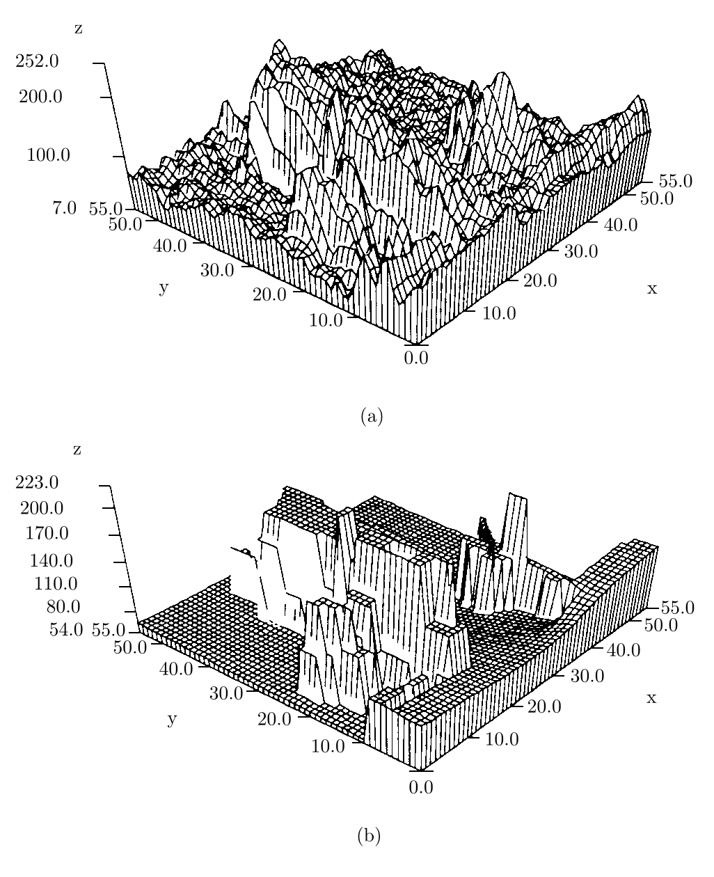
Figure 5. Scale-space using anisotropic diffusion profile $\sigma(s)=\frac{s}{1+s^{2}/s^{2}_{0}}.$ Three dimensional plot of the brightness of Fig. 12 in [35]. (a) Original image, (b) after smoothing with anisotropic diffusion.

We now restate Theorem 1.2 only for Case I. The proof of this appears in Subsection 4.2.

Theorem 3.4.

Let $\Omega$ and $M_{0}$ be as in Theorem 3.1. If $M_{0}<s_{0}$, then (1.2) has a unique solution $u\in C^{2+\alpha,1+\alpha/2}(\bar{\Omega}_{T})$ satisfying $\|Du\|_{L^{\infty}(\Omega_{T})}=\|Du_{0}\|_{L^{\infty}(\Omega)}$.

For the given initial datum $u_{0}$ with $M_{0}<s_{0}$, by Theorem 3.1, there are infinitely many Lipschitz solutions to problem (1.2). On the other hand, by the theorem here, we have a special Lipschitz solution $u$ to (1.2), which is also classical. It may be interesting to observe that none of the Lipschitz solutions from Theorem 3.1 coincide with this special solution $u$.

3.2. Case II: Höllig type of equations

In this case, we impose the following structural condition on the profile $\sigma(s).$

Hypothesis (H): (See Figures 2, 3 and 7.)

• There exist two numbers $s_{2}>s_{1}>0$ such that

  $$f\in C^{0}([0,\infty))\cap C^{1+\alpha}([0,s_{1}^{2})\cup(s_{2}^{2},\infty)).$$

• $\sigma^{\prime}(s)>0\;\;\forall s\in[0,s_{1})\cup(s_{2},\infty)$, $\sigma(s_{1})>\sigma(s_{2})\geq 0$, $\lambda\leq\sigma^{\prime}(s)\leq\Lambda\;\;\forall s\geq 2s_{2}$, where $\Lambda\geq\lambda>0$ are constants.

• Let $s_{1}^{*}\in[0,s_{1})$ and $s_{2}^{*}\in(s_{2},\infty)$ denote the unique numbers with $\sigma(s_{1}^{*})=\sigma(s_{2})$ and $\sigma(s_{2}^{*})=\sigma(s_{1})$, respectively.

Note that the cases $\sigma(s_{2})>0$ and $\sigma(s_{2})=0$ correspond to Figures 2 and 3, respectively. In addition to Hypothesis (H), if we suppose $\sigma(s)\geq 0$ for all $s\in(s_{1},s_{2})$, then $A(p)\cdot p\geq 0$ for all $p\in\mathbb{R}^{n}$, and so (2.9) is satisfied by any Lipschitz solution $u$ to (1.2); but we do not explicitly assume such positivity for Case II unless otherwise stated.

With Hypothesis (H), for each $r\in(\sigma(s_{2}),\sigma(s_{1}))$, let $s_{-}(r)\in(s_{1}^{*},s_{1})$ and $s_{+}(r)\in(s_{2},s_{2}^{*})$ denote the unique numbers with $r=\sigma(s_{\pm}(r))$.

The following theorem is the second main result of this paper that generalizes those of [21, 44] to any dimension $n\geq 1$.

Theorem 3.5.

Let $M_{0}=\|Du_{0}\|_{L^{\infty}(\Omega)}$, $M_{0}^{\prime}=\min\{M_{0},s_{1}\}$, and $|Du_{0}(x_{0})|\in(s_{1}^{*},s_{2}^{*})$ for some $x_{0}\in\Omega.$ Then for each $r\in(\sigma(s_{2}),\sigma(M_{0}^{\prime}))$, there exists a number $l=l_{r}\in(\sigma(s_{2}),r)$ such that for all $\tilde{r}\in(l,r)$ and all but countably many $\bar{r}_{1}\in(\sigma(s_{2}),\tilde{r})$, $\bar{r}_{3}\in(r,\sigma(s_{1}))$, there exist three disjoint open sets $\Omega^{1}_{T},\,\Omega^{2}_{T},\,\Omega^{3}_{T}\subset\Omega_{T}$ with $|\Omega^{1}_{T}\cup\Omega^{2}_{T}\cup\Omega^{3}_{T}|=|\Omega_{T}|$ and infinitely many Lipschitz solutions $u$ to (1.2) satisfying

$$u\in C^{2+\alpha,1+\alpha/2}(\bar{\Omega}^{1}_{T}\cup\bar{\Omega}^{3}_{T}),\quad u_{t}=\operatorname{div}(A(Du))\;\;\mbox{pointwise in}\;\;\Omega_{T}^{1}\cup\Omega_{T}^{3},$$

$$|Du(x,t)|<s_{-}(\bar{r}_{1})\;\;\forall(x,t)\in\Omega_{T}^{1},\quad\Omega_{0}^{\bar{r}_{1}}\subset\partial\Omega_{T}^{1},$$

$$|Du(x,t)|>s_{+}(\bar{r}_{3})\;\;\forall(x,t)\in\Omega_{T}^{3},\quad\Omega_{0}^{\bar{r}_{3}}\subset\partial\Omega_{T}^{3},$$

$$|S|+|L|=|\Omega^{2}_{T}|,\;\;|S|>0,\;\;|L|>0,$$

where

$$\Omega_{0}^{\bar{r}_{1}}=\{(x,0)\,|\,x\in\Omega,\,|Du_{0}(x)|<s_{-}(\bar{r}_{1})\},$$

$$\Omega_{0}^{\bar{r}_{3}}=\{(x,0)\,|\,x\in\Omega,\,|Du_{0}(x)|>s_{+}(\bar{r}_{3})\},$$

$$S=\{(x,t)\in\Omega_{T}^{2}\;|\;s_{-}(\bar{r}_{1})\leq|Du(x,t)|\leq s_{-}(r)\},$$

and

$$L=\{(x,t)\in\Omega_{T}^{2}\;|\;s_{+}(\tilde{r})\leq|Du(x,t)|\leq s_{+}(\bar{r}_{3})\}.$$

In regard to this theorem, an explanation similar to Remark 3.2 can be made; but we omit this. As a byproduct, we also have the following simple existence result whose proof appears after that of Theorem 3.5.

Corollary 3.6.

For any initial datum $u_{0}\in C^{2+\alpha}(\bar{\Omega})$ with $Du_{0}\cdot\mathbf{n}|_{\partial\Omega}=0$, (1.2) has at least one Lipschitz solution.

We now restate Theorem 1.2 only for Case II.

Theorem 3.7.

Let $\Omega$ be convex and $M_{0}=\|Du_{0}\|_{L^{\infty}(\Omega)}$. Assume further that $f\in C^{3}([0,s_{1}^{2})\cup(s_{2}^{2},\infty))$. If $M_{0}<s_{1}$, then (1.2) has a unique solution $u\in C^{2+\alpha,1+\alpha/2}(\bar{\Omega}_{T})$ satisfying $\|Du\|_{L^{\infty}(\Omega_{T})}=\|Du_{0}\|_{L^{\infty}(\Omega)}$.

Unlike Theorem 3.5 and its corollary, the convexity assumption on $\Omega$ cannot be dropped in this theorem. If $s_{1}^{*}<M_{0}<s_{1}$, Theorems 3.5 and 3.7 apply to give infinitely many Lipschitz solutions and one special Lipschitz (classical) solution to problem (1.2) under the same initial datum $u_{0}$, respectively. However, a subtlety arises when $M_{0}\leq s_{1}^{*}$: Is there a Lipschitz solution to (1.2) other than the classical one in this case? Let us discuss more on this in the remark below.

Remark 3.8 (Breakdown of uniqueness).

In this remark, let $\sigma(s)$ satisfy

(3.2) $$\sigma(s)>0\quad\forall s\in(s_{1},s_{2}]$$

in addition to Hypothesis (H) (as in Figure 2), and let $f$ be as in Theorem 3.7. Then by Corollary 3.6, for any $u_{0}\in C^{2+\alpha}(\bar{\Omega})$ with $Du_{0}\cdot\mathbf{n}|_{\partial\Omega}=0$, problem (1.2) has at least one Lipschitz solution. In particular, if $M_{0}=0$ with $M_{0}:=\|Du_{0}\|_{L^{\infty}(\Omega)}$, that is, $u_{0}$ is constant in $\Omega$, then by Proposition 2.4, the constant function $u\equiv u_{0}$ in $\Omega_{T}$ is a unique solution to (1.2). So a natural question is to ask if there is a number $\tilde{M}_{0}>0$ such that (1.2) has a unique Lipschitz solution for all initial data $u_{0}\in C^{2+\alpha}(\bar{\Omega})$ with $Du_{0}\cdot\mathbf{n}|_{\partial\Omega}=0$ and $M_{0}\leq\tilde{M}_{0}$. To address this question, define

$$M^{*}_{0}=\sup\left\{\tilde{M}_{0}\geq 0\,\Big{|}\,\begin{array}[]{l}\mbox{$\forall u_{0}\in C^{2+\alpha}(\bar{\Omega})$ with $Du_{0}\cdot\mathbf{n}|_{\partial\Omega}=0$ and}\\ \mbox{$M_{0}\leq\tilde{M}_{0}$, (\ref{ib-P}) has a unique Lipschitz solution}\end{array}\right\},$$

which we may call as the critical threshold of uniqueness (CTU) for (1.2). The CTU $M^{*}_{0}$ may depend not only on the profile $\sigma(s)$ but also on the dimension $n$, final time $T$, and domain $\Omega$ of problem (1.2). By Theorem 3.5, we have an estimate:

$$0\leq M^{*}_{0}\leq s^{*}_{1},$$

which is valid for all dimensions $n\geq 1$, final times $T>0$, and domains $\Omega$ satisfying (1.6). Our question now boils down to the point of asking if $M^{*}_{0}>0$.

When $n=1$, the answer is affirmative; in this case, the CTU $M^{*}_{0}$ is positive and depends only on the profile $\sigma(s)$. This fact can be derived by using an a priori estimate on the spatial derivatives of Lipschitz solutions. From [22], when $n=1$, any Lipschitz solution $u$ to (1.2) satisfies

(3.3) $$\|u_{x}\|_{L^{\infty}(\Omega_{T})}\leq\frac{\|\sigma(|u_{0}^{\prime}|)\|_{L^{\infty}(\Omega)}}{c},$$

where $c:=\inf_{s\in(0,\infty)}\frac{\sigma(s)}{s}>0$, by Hypothesis (H) and (3.2). Note

$$\frac{\sigma(s_{1}^{*})}{s_{1}}>\frac{\sigma(s_{2})}{s_{2}}\geq c\,;$$

that is, $\sigma(s_{1}^{*})>cs_{1}$. As $\sigma(0)=0$ and $\sigma(s)$ is strictly increasing on $s\in[0,s_{1}^{*}]$, there is a unique number $M^{l}_{0}\in(0,s_{1}^{*})$ with $\sigma(M^{l}_{0})=cs_{1}$. Suppose now that $\|u_{0}^{\prime}\|_{L^{\infty}(\Omega)}<M^{l}_{0}$. Then by Theorem 3.7, there exists a classical solution $\tilde{u}\in C^{2+\alpha,1+\alpha/2}(\bar{\Omega}_{T})$ to (1.2) with $\|\tilde{u}_{x}\|_{L^{\infty}(\Omega_{T})}=\|u_{0}^{\prime}\|_{L^{\infty}(\Omega)}<M^{l}_{0}.$ On the other hand, if $u$ is any Lipschitz solution to (1.2), we have from (3.3) that $\|u_{x}\|_{L^{\infty}(\Omega_{T})}<s_{1}.$ Modifying the profile $\sigma(s)$ to the right of the threshold $\max\{\|u_{0}^{\prime}\|_{L^{\infty}(\Omega)},\|u_{x}\|_{L^{\infty}(\Omega_{T})}\}<s_{1}$, both $\tilde{u}$ and $u$ become Lipschitz solutions to some uniformly parabolic problem of type (1.2) with monotone flux under the same initial datum $u_{0}$. By Proposition 2.3, we thus have $\tilde{u}\equiv u$ in $\Omega_{T}$; hence, the Lipschitz solution $\tilde{u}$ to (1.2) is unique. Therefore, we have an improved estimate for the CTU $M^{*}_{0}$ in $n=1$:

$$0<M^{l}_{0}\leq M^{*}_{0}\leq s^{*}_{1}.$$

As a toy example for $n=1$, we consider the general piecewise linear profile $\sigma(s)$ of the Höllig type. Let $s_{1},\,s_{2},\,k_{1},\,k_{2}$ and $k_{3}$ be positive numbers with $s_{2}>s_{1}$ and $-k_{2}(s_{2}-s_{1})+k_{1}s_{1}>0$. Let us take

$$\sigma(s)=\left\{\begin{array}[]{ll}k_{1}s,&0\leq s\leq s_{1},\\ -k_{2}(s-s_{1})+k_{1}s_{1},&s_{1}\leq s\leq s_{2},\\ k_{3}(s-s_{2})-k_{2}(s_{2}-s_{1})+k_{1}s_{1},&s\geq s_{2};\end{array}\right.$$

then, if $-k_{2}(s_{2}-s_{1})+k_{1}s_{1}<k_{3}s_{2}$, we have

$$0<-s_{1}\frac{k_{2}}{k_{1}}+\frac{s_{1}^{2}}{s_{2}}\big{(}1+\frac{k_{2}}{k_{1}}\big{)}=M^{l}_{0}\leq M^{*}_{0}\leq s^{*}_{1}=-s_{2}\frac{k_{2}}{k_{1}}+s_{1}\big{(}1+\frac{k_{2}}{k_{1}}\big{)},$$

or if $-k_{2}(s_{2}-s_{1})+k_{1}s_{1}\geq k_{3}s_{2}$, it follows that

$$0<s_{1}\frac{k_{3}}{k_{1}}=M^{l}_{0}\leq M^{*}_{0}\leq s^{*}_{1}=-s_{2}\frac{k_{2}}{k_{1}}+s_{1}\big{(}1+\frac{k_{2}}{k_{1}}\big{)}.$$

Unfortunately, estimate (3.3) from [22] is not directly generalized to dimensions $n\geq 2$. However, we still expect that the CTU $M^{*}_{0}>0$ even in dimensions $n\geq 2$ for all $T>0$ as long as $\Omega$ is convex. Since this study is beyond the scope of this paper, we leave it to the interested readers.

4. Some useful results

This section prepares some essential ingredients for the proofs of existence theorems, Theorems 3.1 and 3.5.

4.1. Uniformly parabolic equations

We refer to the standard references (e.g., [29, 30]) for some notations concerning functions and domains of class $C^{k+\alpha}$ with an integer $k\geq 0$.

Assume $\tilde{f}\in C^{1+\alpha}([0,\infty))$ is a function satisfying

(4.1) $$\theta\leq\tilde{f}(s)+2s\tilde{f}^{\prime}(s)\leq\Theta\quad\forall\;s\geq 0,$$

where $\Theta\geq\theta>0$ are constants. This condition is equivalent to $\theta\leq(s\tilde{f}(s^{2}))^{\prime}\leq\Theta$ for all $s\in\mathbb{R};$ hence, $\theta\leq\tilde{f}(s)\leq\Theta$ for all $s\geq 0.$ Let

$$\tilde{A}(p)=\tilde{f}(|p|^{2})p\quad(p\in\mathbb{R}^{n}).$$

Then we have

$$\tilde{A}^{i}_{p_{j}}(p)=\tilde{f}(|p|^{2})\delta_{ij}+2\tilde{f}^{\prime}(|p|^{2})p_{i}p_{j}\quad(i,j=1,2,\cdots,n;\;p\in\mathbb{R}^{n})$$

and hence the uniform ellipticity condition:

(4.2) $$\theta|q|^{2}\leq\sum_{i,j=1}^{n}\tilde{A}^{i}_{p_{j}}(p)q_{i}q_{j}\leq\Theta|q|^{2}\quad\forall\;p,\;q\in\mathbb{R}^{n}.$$

Theorem 4.1.

Assume $(\ref{assume-1})$. Then the initial-Neumann boundary value problem

(4.3) $$\begin{cases}u_{t}=\operatorname{div}(\tilde{A}(Du))&\mbox{in }\Omega_{T},\\ {\partial u}/{\partial\mathbf{n}}=0&\mbox{on }\partial\Omega\times(0,T),\\ u(x,0)=u_{0}(x)&\mbox{for }x\in\Omega\end{cases}$$

has a unique solution $u\in C^{2+\alpha,1+\alpha/2}(\bar{\Omega}_{T})$. Moreover, if $\tilde{f}\in C^{3}([0,\infty))$ and $\Omega$ is convex, then the gradient maximum principle holds:

(4.4) $$\|Du\|_{L^{\infty}(\Omega_{T})}=\|Du_{0}\|_{L^{\infty}(\Omega)}.$$

Proof.

1. As problem (4.3) is uniformly parabolic by (4.2), the existence of unique classical solution $u$ in $C^{2+\alpha,1+\alpha/2}(\bar{\Omega}_{T})$ follows from the standard theory; see [30, Theorem 13.24].

2. To prove the gradient maximum principle (4.4), assume hereafter $\tilde{f}\in C^{3}([0,\infty))$ and $\Omega$ is convex. Note that, since $\tilde{A}\in C^{3}(\mathbb{R}^{n})$, a standard bootstrap argument based on the regularity theory of linear parabolic equations [29, 30] shows that the solution $u$ has all continuous partial derivatives $u_{x_{i}x_{j}x_{k}}$ and $u_{x_{i}t}$ within $\Omega_{T}$ for $1\leq i,j,k\leq n.$

3. Let $v=|Du|^{2}.$ Then, within $\Omega_{T},$ we compute

$$\Delta v=2Du\cdot D(\Delta u)+2|D^{2}u|^{2},$$

$$u_{t}=\operatorname{div}(\tilde{A}(Du))=\operatorname{div}(\tilde{f}(v)Du)=\tilde{f}^{\prime}(v)Dv\cdot Du+\tilde{f}(v)\Delta u,$$

$$Du_{t}=\tilde{f}^{\prime\prime}(v)(Dv\cdot Du)Dv+\tilde{f}^{\prime}(v)(D^{2}u)Dv$$

$$+\tilde{f}^{\prime}(v)(D^{2}v)Du+\tilde{f}^{\prime}(v)(\Delta u)Dv+\tilde{f}(v)D(\Delta u).$$

Putting these equations into $v_{t}=2Du\cdot Du_{t}$, we obtain

(4.5) $$v_{t}-\mathcal{L}(v)-B\cdot Dv=-2\tilde{f}(|Du|^{2})|D^{2}u|^{2}\leq 0\quad\mbox{in $\Omega_{T}$,}$$

where operator $\mathcal{L}(v)$ and coefficient $B$ are defined by

$$\mathcal{L}(v)=\tilde{f}(|Du|^{2})\Delta v+2\tilde{f}^{\prime}(|Du|^{2})Du\cdot(D^{2}v)Du,$$

$$B=2\tilde{f}^{\prime\prime}(v)(Dv\cdot Du)Du+2\tilde{f}^{\prime}(v)(D^{2}u)Du+2\tilde{f}^{\prime}(v)(\Delta u)Du.$$

We write $\mathcal{L}(v)=\sum_{i,j=1}^{n}a_{ij}v_{x_{i}x_{j}},$ with coefficients $a_{ij}=a_{ij}(x,t)$ given by

$$a_{ij}=\tilde{A}^{i}_{p_{j}}(Du)=\tilde{f}(|Du|^{2})\delta_{ij}+2\tilde{f}^{\prime}(|Du|^{2})u_{x_{i}}u_{x_{j}}\quad(i,j=1,\cdots,n).$$

Note that on $\bar{\Omega}_{T}$ all eigenvalues of the matrix $(a_{ij})$ lie in $[\theta,\Theta]$.

4. We show

$$\max_{(x,t)\in\bar{\Omega}_{T}}v(x,t)=\max_{x\in\bar{\Omega}}v(x,0),$$

which proves (4.4). We prove this by contradiction. Suppose

(4.6) $$M:=\max_{(x,t)\in\bar{\Omega}_{T}}v(x,t)>\max_{x\in\bar{\Omega}}v(x,0).$$

Let $(x_{0},t_{0})\in\bar{\Omega}_{T}$ be such that $v(x_{0},t_{0})=M;$ then $t_{0}>0.$ If $x_{0}\in\Omega$, then the strong maximum principle applied to (4.5) would imply that $v$ is constant on $\Omega_{t_{0}},$ which yields $v(x,0)\equiv M$ on $\bar{\Omega}$, a contradiction to (4.6). Consequently $x_{0}\in\partial\Omega$ and thus $v(x_{0},t_{0})=M>v(x,t)$ for all $(x,t)\in\Omega_{T}.$ We can then apply Hopf’s Lemma for parabolic equations [36] to (4.5) to deduce $\partial v(x_{0},t_{0})/\partial\mathbf{n}>0.$ However, mainly due the convexity of $\Omega$, a result of [1, Lemma 2.1] (see also [23, Theorem 2]) asserts that $\partial v/\partial\mathbf{n}\leq 0$ on $\partial\Omega\times[0,T],$ which gives a desired contradiction. ∎

4.2. Modification of the profile functions

The following elementary results can be proved in a similar way as in [8, 43]; we omit the proofs.

Lemma 4.2 (Case I: Perona-Malik type; see Figure 6).

Assume Hypothesis (PM). For every $0<r_{1}<r_{2}<\sigma(s_{0})$, there exists a function $\tilde{\sigma}\in C^{3}([0,\infty))$ such that

(4.7) $$\begin{cases}\tilde{\sigma}(s)=\sigma(s),&0\leq s\leq s_{-}(r_{1}),\\ \tilde{\sigma}(s)<\sigma(s),&s_{-}(r_{1})<s<s_{+}(r_{2}),\\ \theta\leq\tilde{\sigma}^{\prime}(s)\leq\Theta,&0\leq s<\infty\end{cases}$$

for some constants $\Theta\geq\theta>0.$ With such a function $\tilde{\sigma}$, define $\tilde{f}(s)=\tilde{\sigma}(\sqrt{s})/\sqrt{s}$ ($s>0$) and $\tilde{f}(0)=f(0);$ then $\tilde{f}\in C^{3}([0,\infty))$ fulfills condition $(\ref{para})$.

Figure 6. Case I: Perona-Malik type of profile $\sigma(s)$ and modified function $\tilde{\sigma}(s)$.

Lemma 4.3 (Case II: Höllig type; see Figure 7).

Assume Hypothesis (H). For every $\sigma(s_{2})<r_{1}<r_{2}<\sigma(s_{1})$, there exists a function $\tilde{\sigma}\in C^{1+\alpha}([0,\infty))$ such that

(4.8) $$\begin{cases}\tilde{\sigma}(s)=\sigma(s),&0\leq s\leq s_{-}(r_{1}),\\ \tilde{\sigma}(s)<\sigma(s),&s_{-}(r_{1})<s\leq s_{-}(r_{2}),\\ \tilde{\sigma}(s)>\sigma(s),&s_{+}(r_{1})\leq s<s_{+}(r_{2}),\\ \tilde{\sigma}(s)=\sigma(s),&s_{+}(r_{2})\leq s<\infty,\\ \theta\leq\tilde{\sigma}^{\prime}(s)\leq\Theta,&0\leq s<\infty\end{cases}$$

for some constants $\Theta\geq\theta>0.$ With such a function $\tilde{\sigma}$, define $\tilde{f}(s)=\tilde{\sigma}(\sqrt{s})/\sqrt{s}$ ($s>0$) and $\tilde{f}(0)=f(0);$ then $\tilde{f}\in C^{1+\alpha}([0,\infty))$ fulfills condition $(\ref{para})$. Moreover, if $f\in C^{3}([0,s_{1}^{2})\cup(s_{2}^{2},\infty))$ in addition, then $\tilde{\sigma},\,\tilde{f}$ can be chosen to be also in $C^{3}([0,\infty))$.

Figure 7. Case II: Höllig type of profile $\sigma(s)$ and modified function $\tilde{\sigma}(s)$.

4.3. Proofs of Theorems 3.4 and 3.7

Let $M_{0}=\|Du_{0}\|_{L^{\infty}(\Omega)}.$ In Case I (Perona-Malik type), we have $0<M_{0}<s_{0}$; so we can select $0<r_{1}<r_{2}<\sigma(s_{0})$ such that $s_{-}(r_{1})=M_{0}.$ In Case II (Höllig type), we have $0<M_{0}<s_{1}$; so we can select $\sigma(s_{2})<r_{1}<r_{2}<\sigma(s_{1})$ such that $s_{-}(r_{1})\geq M_{0}.$ Use such a choice of $r_{1},\,r_{2}$ in Lemma 4.2 (Case I), Lemma 4.3 (Case II) to obtain a $C^{3}$ function $\tilde{f}$ as stated in the lemma. Let $\tilde{A}(p)=\tilde{f}(|p|^{2})p.$ For this $\tilde{A}(p)$, problem (4.3) is uniformly parabolic; hence, by Theorem 4.1, (4.3) has a unique solution $u\in C^{2+\alpha,1+\alpha/2}(\bar{\Omega}_{T})$ satisfying

$$\|Du\|_{L^{\infty}(\Omega_{T})}=\|Du_{0}\|_{L^{\infty}(\Omega)}.$$

Since $\tilde{A}(p)=A(p)$ on $|p|\leq s_{-}(r_{1})$ and $s_{-}(r_{1})\geq M_{0}$, it follows that $\tilde{A}(Du(x,t))=A(Du(x,t))$ in $\Omega_{T};$ this proves $u$ is a classical solution to problem (1.2). On the other hand, we easily see that any classical solution to (1.2) satisfying $\|Du\|_{L^{\infty}(\Omega_{T})}=M_{0}$ is also a classical solution to (4.3) and hence must be unique. This completes the proofs of Theorems 3.4 and 3.7.

4.4. Right inverse of the divergence operator

To deal with linear constraint $\operatorname{div}v=u$, we follow an argument of [5, Lemma 4] to construct a right inverse $\mathcal{R}$ of the divergence operator: $\operatorname{div}\mathcal{R}=Id$ (in the sense of distributions in $\Omega_{T}$). For the purpose of this paper, the construction of $\mathcal{R}$ is restricted to box domains, by which we mean domains given by $Q=J_{1}\times J_{2}\times\cdots\times J_{n}$, where $J_{i}=(a_{i},b_{i})\subset\mathbb{R}$ is a finite open interval.

Given a box $Q$, we define a linear operator $\mathcal{R}_{n}\colon L^{\infty}(Q)\to L^{\infty}(Q;\mathbb{R}^{n})$ inductively on dimension $n$ as follows. If $n=1$, for $u\in L^{\infty}(J_{1})$, we define $v=\mathcal{R}_{1}u$ by

$$v(x_{1})=\int_{a_{1}}^{x_{1}}u(s)ds\quad(x_{1}\in J_{1}).$$

Assume $n=2$. Let $u\in L^{\infty}(J_{1}\times J_{2}).$ Set $\tilde{u}(x_{1})=\int_{a_{2}}^{b_{2}}u(x_{1},s)\,ds$ for $x_{1}\in J_{1}.$ Then $\tilde{u}\in L^{\infty}(J_{1}).$ Let $\tilde{v}=\mathcal{R}_{1}\tilde{u}$; that is,

$$\tilde{v}(x_{1})=\int_{a_{1}}^{x_{1}}\tilde{u}(s)ds=\int_{a_{1}}^{x_{1}}\int_{a_{2}}^{b_{2}}u(s,\tau)\,d\tau ds\quad(x_{1}\in J_{1}).$$

Let $\rho_{2}\in C^{\infty}_{c}(a_{2},b_{2})$ be such that $0\leq\rho_{2}(s)\leq\frac{C_{0}}{b_{2}-a_{2}}$ and $\int_{a_{2}}^{b_{2}}\rho_{2}(s)ds=1.$ Define $v=\mathcal{R}_{2}u\in L^{\infty}(J_{1}\times J_{2};\mathbb{R}^{2})$ by $v=(v^{1},v^{2})$ with $v^{1}(x_{1},x_{2})=\rho_{2}(x_{2})\tilde{v}(x_{1})$ and

$$v^{2}(x_{1},x_{2})=\int_{a_{2}}^{x_{2}}u(x_{1},s)ds-\tilde{u}(x_{1})\int_{a_{2}}^{x_{2}}\rho_{2}(s)ds.$$

Note that if $u\in W^{1,\infty}(J_{1}\times J_{2})$ then $\tilde{u}\in W^{1,\infty}(J_{1})$; hence $v=\mathcal{R}_{2}u\in W^{1,\infty}(J_{1}\times J_{2};\mathbb{R}^{2})$ and $\operatorname{div}v=u$ a.e. in $J_{1}\times J_{2}.$ Moreover, if $u\in C^{1}(\overline{J_{1}\times J_{2}})$ then $v$ is in $C^{1}(\overline{J_{1}\times J_{2}};\mathbb{R}^{2}).$

Assume that we have defined the operator $\mathcal{R}_{n-1}$. Let $u\in L^{\infty}(Q)$ with $Q=J_{1}\times J_{2}\times\cdots\times J_{n}$ and $x=(x^{\prime},x_{n})\in Q$, where $x^{\prime}\in Q^{\prime}=J_{1}\times\cdots\times J_{n-1}$ and $x_{n}\in J_{n}.$ Set $\tilde{u}(x^{\prime})=\int_{a_{n}}^{b_{n}}u(x^{\prime},s)\,ds$ for $x^{\prime}\in Q^{\prime}.$ Then $\tilde{u}\in L^{\infty}(Q^{\prime}).$ By the assumption, $\tilde{v}=\mathcal{R}_{n-1}\tilde{u}\in L^{\infty}(Q^{\prime};\mathbb{R}^{n-1})$ is defined. Write $\tilde{v}(x^{\prime})=(Z^{1}(x^{\prime}),\cdots,Z^{n-1}(x^{\prime})),$ and let $\rho_{n}\in C^{\infty}_{c}(a_{n},b_{n})$ be a function satisfying $0\leq\rho_{n}(s)\leq\frac{C_{0}}{b_{n}-a_{n}}$ and $\int_{a_{n}}^{b_{n}}\rho_{n}(s)ds=1.$ Define $v=\mathcal{R}_{n}u\in L^{\infty}(Q;\mathbb{R}^{n})$ as follows. For $x=(x^{\prime},x_{n})\in Q,$ $v(x)=(v^{1}(x),v^{2}(x),\cdots,v^{n}(x))$ is defined by

$$\begin{split}&v^{k}(x^{\prime},x_{n})=\rho_{n}(x_{n})Z^{k}(x^{\prime})\quad(k=1,2,\cdots,n-1),\\ &v^{n}(x^{\prime},x_{n})=\int_{a_{n}}^{x_{n}}u(x^{\prime},s)ds-\tilde{u}(x^{\prime})\int_{a_{n}}^{x_{n}}\rho_{n}(s)ds.\end{split}$$

Then $\mathcal{R}_{n}\colon L^{\infty}(Q)\to L^{\infty}(Q;\mathbb{R}^{n})$ is a well-defined linear operator; moreover,

(4.9) $$\|\mathcal{R}_{n}u\|_{L^{\infty}(Q)}\leq C_{n}\,(|J_{1}|+\cdots+|J_{n}|)\|u\|_{L^{\infty}(Q)},$$

where $C_{n}>0$ is a constant depending only on $n.$

As in the case $n=2$, we see that if $u\in W^{1,\infty}(Q)$ then $v=\mathcal{R}_{n}u\in W^{1,\infty}(Q;\mathbb{R}^{n})$ and $\operatorname{div}v=u$ a.e. in $Q$. Also, if $u\in C^{1}(\bar{Q})$ then $v=\mathcal{R}_{n}u$ is in $C^{1}(\bar{Q};\mathbb{R}^{n}).$ Moreover, if $u\in W^{1,\infty}_{0}(Q)$ satisfies $\int_{Q}u(x)dx=0$, then one can easily show that $v=\mathcal{R}_{n}u\in W_{0}^{1,\infty}(Q;\mathbb{R}^{n}).$

Let $I$ be a finite open interval in $\mathbb{R}$. We now extend the operator $\mathcal{R}_{n}$ to an operator $\mathcal{R}$ on $L^{\infty}(Q\times I)$ by defining, for a.e. $(x,t)\in Q\times I$,

(4.10) $$(\mathcal{R}u)(x,t)=(\mathcal{R}_{n}u(\cdot,t))(x)\quad\forall\;u\in L^{\infty}(Q\times I).$$

Then $\mathcal{R}\colon L^{\infty}(Q\times I)\to L^{\infty}(Q\times I;\mathbb{R}^{n})$ is a bounded linear operator.

We have the following result.

Theorem 4.4.

Let $u\in W^{1,\infty}_{0}(Q\times I)$ satisfy $\int_{Q}u(x,t)\,dx=0$ for all $t\in I$. Then $v=\mathcal{R}u\in W^{1,\infty}_{0}(Q\times I;\mathbb{R}^{n})$, $\operatorname{div}v=u$ a.e. in $Q\times I$, and

(4.11) $$\|v_{t}\|_{L^{\infty}(Q\times I)}\leq C_{n}\,(|J_{1}|+\cdots+|J_{n}|)\|u_{t}\|_{L^{\infty}(Q\times I)},$$

where $Q=J_{1}\times\cdots\times J_{n}$ and $C_{n}$ is the same constant as in $(\ref{div-0})$. Moreover, if $u\in C^{1}(\overline{Q\times I})$ then $v=\mathcal{R}u\in C^{1}(\overline{Q\times I};\mathbb{R}^{n}).$

Proof.

Given $u\in W^{1,\infty}_{0}(Q\times I)$, let $v=\mathcal{R}u.$ We easily verify that $v$ is Lipschitz continuous in $t$ and hence $v_{t}$ exists. It also follows that $v_{t}=\mathcal{R}(u_{t}).$ Clearly, if $\int_{Q}u(x,t)dx=0$ then $v(x,t)=0$ whenever $t\in\partial I$ or $x\in\partial Q$. This proves $v\in W^{1,\infty}_{0}(Q\times I;\mathbb{R}^{n})$ and the estimate (4.11) follows from (4.9). Finally, from the definition of $\mathcal{R}u$, we see that if $u\in C^{1}(\overline{Q\times I})$ then $v=\mathcal{R}u\in C^{1}(\overline{Q\times I};\mathbb{R}^{n}).$ ∎

5. Geometry of the relevant matrix sets

Let $A(p)$ be given by (1.3). We assume Hypothesis (PM) or (H) unless one is chosen specifically. Recall the definition (2.3) with $l=0$:

(5.1) $$K_{0}=K(0)=\left\{\begin{pmatrix}p&c\\ B&A(p)\end{pmatrix}\,\Big{|}\,p\in\mathbb{R}^{n},\,c\in\mathbb{R},\,B\in\mathbb{M}^{n\times n},\,\operatorname{tr}B=0\right\}.$$

Under Hypothesis (PM) or (H), certain structures of the set $K_{0}$ turn out to be still quite useful, especially when it comes to the relaxation of homogeneous partial differential inclusion $\nabla\omega(z)\in K_{0}$ with $z=(x,t)$ and $\omega=(\varphi,\psi)$. We investigate these structures and establish such relaxation results throughout this section.

5.1. Geometry of the matrix set $K_{0}$

We study some subsets of $K_{0}$, depending on the different types of profiles.

Case I: Hypothesis (PM)

(See Figure 6.) In this case, we assume the following. Fix any two numbers $0<r_{1}<r_{2}<\sigma(s_{0})$, and let $F_{0}=F_{r_{1},r_{2}}(0)$ be the subset of $K_{0}$ defined by

$$F_{0}=\left\{\begin{pmatrix}p&c\\ B&A(p)\end{pmatrix}\,\Big{|}\,\begin{array}[]{l}p\in\mathbb{R}^{n},\,|p|\in(s_{-}(r_{1}),s_{-}(r_{2}))\cup(s_{+}(r_{2}),s_{+}(r_{1})),\\ c\in\mathbb{R},\,B\in\mathbb{M}^{n\times n},\,\operatorname{tr}B=0\end{array}\right\}.$$

We decompose the set $F_{0}$ into two disjoint subsets as follows:

$$F_{-}=\left\{\begin{pmatrix}p&c\\ B&A(p)\end{pmatrix}\,\Big{|}\,\begin{array}[]{l}p\in\mathbb{R}^{n},\,|p|\in(s_{-}(r_{1}),s_{-}(r_{2})),\\ c\in\mathbb{R},\,B\in\mathbb{M}^{n\times n},\,\operatorname{tr}B=0\end{array}\right\},$$

$$F_{+}=\left\{\begin{pmatrix}p&c\\ B&A(p)\end{pmatrix}\,\Big{|}\,\begin{array}[]{l}p\in\mathbb{R}^{n},\,|p|\in(s_{+}(r_{2}),s_{+}(r_{1})),\\ c\in\mathbb{R},\,B\in\mathbb{M}^{n\times n},\,\operatorname{tr}B=0\end{array}\right\}.$$

Case II: Hypothesis (H)

(See Figure 7.) In this case, we assume the following. Fix any two numbers $\sigma(s_{2})<r_{1}<r_{2}<\sigma(s_{1})$, and let $F_{0}=F_{r_{1},r_{2}}(0)$ be the subset of $K_{0}$ given by

$$F_{0}=\left\{\begin{pmatrix}p&c\\ B&A(p)\end{pmatrix}\,\Big{|}\,\begin{array}[]{l}p\in\mathbb{R}^{n},\,|p|\in(s_{-}(r_{1}),s_{-}(r_{2}))\cup(s_{+}(r_{1}),s_{+}(r_{2})),\\ c\in\mathbb{R},\,B\in\mathbb{M}^{n\times n},\,\operatorname{tr}B=0\end{array}\right\}.$$

The set $F_{0}$ is also decomposed into two disjoint subsets as follows:

$$F_{-}=\left\{\begin{pmatrix}p&c\\ B&A(p)\end{pmatrix}\,\Big{|}\,\begin{array}[]{l}p\in\mathbb{R}^{n},\,|p|\in(s_{-}(r_{1}),s_{-}(r_{2})),\\ c\in\mathbb{R},\,B\in\mathbb{M}^{n\times n},\,\operatorname{tr}B=0\end{array}\right\},$$

$$F_{+}=\left\{\begin{pmatrix}p&c\\ B&A(p)\end{pmatrix}\,\Big{|}\,\begin{array}[]{l}p\in\mathbb{R}^{n},\,|p|\in(s_{+}(r_{1}),s_{+}(r_{2})),\\ c\in\mathbb{R},\,B\in\mathbb{M}^{n\times n},\,\operatorname{tr}B=0\end{array}\right\}.$$

In order to study the homogeneous differential inclusion $\nabla\omega(z)\in K_{0}$, we first scrutinize the rank-one structure of the set $F_{0}\subset K_{0}$. We introduce the following notation.

Definition 5.1.

For a given set $E\subset\mathbb{M}^{(1+n)\times(n+1)}$, $L(E)$ is defined to be the set of all matrices $\xi\in\mathbb{M}^{(1+n)\times(n+1)}$ that are not in $E$ but are representable by $\xi=\lambda\xi_{1}+(1-\lambda)\xi_{2}$ for some $\lambda\in(0,1)$ and $\xi_{1},\xi_{2}\in E$ with $\operatorname{rank}(\xi_{1}-\xi_{2})=1$, or equivalently,

$$L(E)=\{\xi\not\in E\;|\;\mbox{$\xi+t_{\pm}\eta\in E$ for some $t_{-}<0<t_{+}$ and $\operatorname{rank}\eta=1$}\}.$$

For the matrix set $F_{0}$, we define

$$R(F_{0})=\bigcup_{\xi_{\pm}\in F_{\pm},\,\mathrm{rank}(\xi_{+}-\xi_{-})=1}(\xi_{-},\xi_{+}),$$

where $(\xi_{-},\xi_{+})$ is the open line segment in $\mathbb{M}^{(1+n)\times(n+1)}$ joining $\xi_{\pm}$. Then from careful analyses, one can actually deduce

(5.2) $$L(F_{0})=R(F_{0})\cup L(F_{+})\quad\mbox{in {\bf Case I}}$$

and

(5.3) $$L(F_{0})=R(F_{0})\quad\mbox{in {\bf Case II}}.$$

In (5.2), due to the backward nature of $\sigma(s)$ on $(s_{+}(r_{2}),s_{+}(r_{1}))$ for Case I, the set $L(F_{+})$ turns out to be non-empty. On the other hand, as only forward parts of $\sigma$ are involved in $F_{0}$ for Case II, no such set appears in (5.3). Regardless of this discrepancy, we can only stick to the analysis of the set $R(F_{0})$ for both cases towards the existence results, Theorems 3.1 and 3.5.

We perform the step-by-step analysis of the set $R(F_{0})$ for both cases simultaneously.

5.1.1. Alternate expression for $R(F_{0})$

We investigate more specific criteria for matrices in $R(F_{0})$.

Lemma 5.2.

Let $\xi\in\mathbb{M}^{(1+n)\times(n+1)}$. Then $\xi\in R(F_{0})$ if and only if there exist numbers $t_{-}<0<t_{+}$ and vectors $q,\,\gamma\in\mathbb{R}^{n}$ with $|q|=1,\,\gamma\cdot q=0$ such that for each $b\in\mathbb{R}\setminus\{0\}$, if $\eta=\begin{pmatrix}q&b\\ \frac{1}{b}q\otimes\gamma&\gamma\end{pmatrix}$, then $\xi+t_{\pm}\eta\in F_{\pm}$.

Proof.

Assume $\xi=\begin{pmatrix}p&c\\ B&\beta\end{pmatrix}\in R(F_{0})$. By definition, $\xi+t_{\pm}\tilde{\eta}\in F_{\pm},$ where $t_{-}<0<t_{+}$ and $\tilde{\eta}$ is a rank-one matrix given by

$$\tilde{\eta}=\begin{pmatrix}a\\ \alpha\end{pmatrix}\otimes(q,\tilde{b})=\begin{pmatrix}aq&a\tilde{b}\\ \alpha\otimes q&\tilde{b}\alpha\end{pmatrix},\quad a^{2}+|\alpha|^{2}\neq 0,\quad\tilde{b}^{2}+|q|^{2}\neq 0,$$

for some $a,\,\tilde{b}\in\mathbb{R}$ and $\alpha,\,q\in\mathbb{R}^{n}$; here $\alpha\otimes q$ denotes the rank-one or zero matrix $(\alpha_{i}q_{j})$ in $\mathbb{M}^{n\times n}$. Condition $\xi+t_{\pm}\tilde{\eta}\in F_{\pm}$ with $t_{-}<0<t_{+}$ is equivalent to the following: For Case I,

(5.4) $$\begin{split}&\operatorname{tr}B=0,\quad\alpha\cdot q=0,\quad A(p+t_{\pm}aq)=\beta+t_{\pm}\tilde{b}\alpha,\\ |p+t&{}_{+}aq|\in(s_{+}(r_{2}),s_{+}(r_{1})),\quad|p+t_{-}aq|\in(s_{-}(r_{1}),s_{-}(r_{2})).\end{split}$$

For Case II,

(5.5) $$\begin{split}&\operatorname{tr}B=0,\quad\alpha\cdot q=0,\quad A(p+t_{\pm}aq)=\beta+t_{\pm}\tilde{b}\alpha,\\ |p+t&{}_{+}aq|\in(s_{+}(r_{1}),s_{+}(r_{2})),\quad|p+t_{-}aq|\in(s_{-}(r_{1}),s_{-}(r_{2})).\end{split}$$

Therefore, $aq\neq 0$. Upon rescaling $\tilde{\eta}$ and $t_{\pm}$, we can assume $a=1$ and $|q|=1$; namely,

$$\tilde{\eta}=\begin{pmatrix}q&\tilde{b}\\ \alpha\otimes q&\tilde{b}\alpha\end{pmatrix},\quad|q|=1,\quad\alpha\cdot q=0.$$

We now let $\gamma=\tilde{b}\alpha$. Let $b\in\mathbb{R}\setminus\{0\}$ and

$$\eta=\begin{pmatrix}q&b\\ \frac{1}{b}\gamma\otimes q&\gamma\end{pmatrix}.$$

From (5.4) or (5.5), it follows that $\xi+t_{\pm}\eta\in F_{\pm}$.

The converse directly follows from the definition of $R(F_{0})$. ∎

5.1.2. Diagonal components of matrices in $R(F_{0})$.

The following gives a description for the diagonal components of matrices in $R(F_{0})$.

Lemma 5.3.

(5.6) $$R(F_{0})=\left\{\begin{pmatrix}p&c\\ B&\beta\end{pmatrix}\,\Big{|}\,c\in\mathbb{R},\,B\in\mathbb{M}^{n\times n},\,\operatorname{tr}B=0,\,(p,\beta)\in\mathcal{S}\right\}$$

for some set $\mathcal{S}=\mathcal{S}_{r_{1},r_{2}}\subset\mathbb{R}^{n+n}$.

Proof.

Let $(c,B),\,(c^{\prime},B^{\prime})\in\mathbb{R}\times\mathbb{M}^{n\times n}$ be such that $\operatorname{tr}B=\operatorname{tr}B^{\prime}=0$, and define

$$\mathcal{S}_{(c,B)}=\left\{(p,\beta)\in\mathbb{R}^{n+n}\,\Big{|}\,\begin{pmatrix}p&c\\ B&\beta\end{pmatrix}\in R(F_{0})\right\},$$

$$\mathcal{S}_{(c^{\prime},B^{\prime})}=\left\{(p,\beta)\in\mathbb{R}^{n+n}\,\Big{|}\,\begin{pmatrix}p&c^{\prime}\\ B^{\prime}&\beta\end{pmatrix}\in R(F_{0})\right\}.$$

It is sufficient to show that $\mathcal{S}_{(c,B)}=\mathcal{S}_{(c^{\prime},B^{\prime})}=:\mathcal{S}.$ Let $(p,\beta)\in\mathcal{S}_{(c,B)}$, that is, $\xi=\begin{pmatrix}p&c\\ B&\beta\end{pmatrix}\in R(F_{0})$. Then $\xi_{\pm}:=\xi+t_{\pm}\eta\in F_{\pm}$ for some $t_{-}<0<t_{+}$ and $\mathrm{rank}\,\eta=1$. Observe that $\xi=\lambda\xi_{+}+(1-\lambda)\xi_{-}$ with $\lambda=\frac{-t_{-}}{t_{+}-t_{-}}\in(0,1)$ and that

$$\xi^{\prime}:=\begin{pmatrix}p&c^{\prime}\\ B^{\prime}&\beta\end{pmatrix}=\xi+\begin{pmatrix}0&\tilde{c}\\ \tilde{B}&0\end{pmatrix}=\lambda\tilde{\xi}_{+}+(1-\lambda)\tilde{\xi}_{-}$$

where $\tilde{c}=c^{\prime}-c$, $\tilde{B}=B^{\prime}-B$, and $\tilde{\xi}_{\pm}=\xi_{\pm}+\begin{pmatrix}0&\tilde{c}\\ \tilde{B}&0\end{pmatrix}$. Since $\xi_{\pm}\in F_{\pm}$ and $\operatorname{tr}\tilde{B}=0$, we have $\tilde{\xi}_{\pm}\in F_{\pm}$, and so $\xi^{\prime}\in R(F_{0})$. This implies $(p,\beta)\in\mathcal{S}_{(c^{\prime},B^{\prime})}$; hence $\mathcal{S}_{(c,B)}\subset\mathcal{S}_{(c^{\prime},B^{\prime})}$. Likewise, $\mathcal{S}_{(c^{\prime},B^{\prime})}\subset\mathcal{S}_{(c,B)}$; that is, $\mathcal{S}_{(c,B)}=\mathcal{S}_{(c^{\prime},B^{\prime})}$. ∎

5.1.3. Selection of approximate collinear rank-one connections for $R(F_{0})$.

We begin with a 2-dimensional description for the rank-one connections of diagonal components of matrices in $R(F_{0})$ in a general form. The following lemma deals with Cases I and II in a parallel manner.

Lemma 5.4.

For all positive numbers $a,b,c$ with $b>a$, there exists a continuous function

$$h_{1}(a,b,c;\cdot,\cdot,\cdot):I^{1}_{a,b,c}=[0,a)\times[0,\infty)\times[0,c)\to[0,\infty)\quad\mbox{\emph{({Case I})}}$$

$$h_{2}(a,b,c;\cdot,\cdot,\cdot):I^{2}_{a,b,c}=[0,a)\times[0,b-a)\times[0,c)\to[0,\infty)\quad\mbox{\emph{({Case II})}}$$

with $h_{i}(a,b,c;0,0,0)=0$ satisfying the following:

Let $\delta_{1},\delta_{2}$ and $\eta$ be any positive numbers with

$$0<a-\delta_{1}<a<b<b+\delta_{2},\quad 0<c-\eta<c,\quad\mbox{\emph{({Case I})}}$$

$$0<a-\delta_{1}<a<b-\delta_{2}<b,\quad 0<c-\eta<c,\quad\mbox{\emph{({Case II})}}$$

and let $R_{1}\in[a-\delta_{1},a]$, $R_{2}\in[b,b+\delta_{2}]$ (Case I), $R_{2}\in[b-\delta_{2},b]$ (Case II), and $\tilde{R}_{1},\tilde{R}_{2}\in[c-\eta,c]$. Suppose $\theta\in[-\pi/2,\pi/2]$ and

$$\begin{split}\Big{(}\tilde{R}_{1}\big{(}&\cos(\frac{\pi}{2}+\theta),\sin(\frac{\pi}{2}+\theta)\big{)}-\tilde{R}_{2}\big{(}\cos(\frac{\pi}{2}-\theta),\sin(\frac{\pi}{2}-\theta)\big{)}\Big{)}\\ &\cdot\Big{(}R_{1}\big{(}\cos(\frac{\pi}{2}+\theta),\sin(\frac{\pi}{2}+\theta)\big{)}-R_{2}\big{(}\cos(\frac{\pi}{2}-\theta),\sin(\frac{\pi}{2}-\theta)\big{)}\Big{)}=0.\end{split}$$

Then $-\frac{\pi}{2}<\theta<\frac{\pi}{2}$, $\tilde{R}_{1}\geq\tilde{R}_{2}$, and

$$\max\Big{\{}\big{|}(0,a)-R_{1}\big{(}\cos(\frac{\pi}{2}+\theta),\sin(\frac{\pi}{2}+\theta)\big{)}\big{|},\,\big{|}(0,b)-R_{2}\big{(}\cos(\frac{\pi}{2}-\theta),\sin(\frac{\pi}{2}-\theta)\big{)}\big{|}$$

$$\big{|}(0,c)-\tilde{R}_{1}\big{(}\cos(\frac{\pi}{2}+\theta),\sin(\frac{\pi}{2}+\theta)\big{)}\big{|},\,\big{|}(0,c)-\tilde{R}_{2}\big{(}\cos(\frac{\pi}{2}-\theta),\sin(\frac{\pi}{2}-\theta)\big{)}\big{|}\Big{\}}$$

$$\leq h_{1}(a,b,c;\delta_{1},\delta_{2},\eta),\quad\emph{({Case I})}$$

$$\max\Big{\{}\big{|}(0,a)-R_{1}\big{(}\cos(\frac{\pi}{2}+\theta),\sin(\frac{\pi}{2}+\theta)\big{)}\big{|},\,\big{|}(0,b)-R_{2}\big{(}\cos(\frac{\pi}{2}-\theta),\sin(\frac{\pi}{2}-\theta)\big{)}\big{|}$$

$$\big{|}(0,c)-\tilde{R}_{1}\big{(}\cos(\frac{\pi}{2}+\theta),\sin(\frac{\pi}{2}+\theta)\big{)}\big{|},\,\big{|}(0,c)-\tilde{R}_{2}\big{(}\cos(\frac{\pi}{2}-\theta),\sin(\frac{\pi}{2}-\theta)\big{)}\big{|}\Big{\}}$$

$$\leq h_{2}(a,b,c;\delta_{1},\delta_{2},\eta).\quad\emph{({Case II})}$$

Proof.

By assumption,

$$0=(\tilde{R}_{1}(-\sin\theta,\cos\theta)-\tilde{R}_{2}(\sin\theta,\cos\theta))\cdot(R_{1}(-\sin\theta,\cos\theta)-R_{2}(\sin\theta,\cos\theta))$$

$$=(-(\tilde{R}_{1}+\tilde{R}_{2})\sin\theta,(\tilde{R}_{1}-\tilde{R}_{2})\cos\theta)\cdot(-(R_{1}+R_{2})\sin\theta,(R_{1}-R_{2})\cos\theta)$$

$$=(\tilde{R}_{1}+\tilde{R}_{2})(R_{1}+R_{2})\sin^{2}\theta+(\tilde{R}_{1}-\tilde{R}_{2})(R_{1}-R_{2})\cos^{2}\theta,$$

that is,

$$(R_{2}-R_{1})(\tilde{R}_{1}-\tilde{R}_{2})\cos^{2}\theta=(R_{1}+R_{2})(\tilde{R}_{1}+\tilde{R}_{2})\sin^{2}\theta;$$

hence, $\theta\neq\pm\frac{\pi}{2}$, $\tilde{R}_{1}\geq\tilde{R}_{2}$, and

$$\theta=\pm\tan^{-1}\left(\sqrt{\frac{(R_{2}-R_{1})(\tilde{R}_{1}-\tilde{R}_{2})}{(R_{1}+R_{2})(\tilde{R}_{1}+\tilde{R}_{2})}}\right).$$

So

$$|\theta|\leq\tan^{-1}\left(\sqrt{\frac{(b-a+\delta_{1}+\delta_{2})\eta}{2(a+b-\delta_{1})(c-\eta)}}\right)=:g_{1}(a,b,c;\delta_{1},\delta_{2},\eta),\;\;\mbox{({Case I})}$$

$$|\theta|\leq\tan^{-1}\left(\sqrt{\frac{(b-a+\delta_{1})\eta}{2(a+b-\delta_{1}-\delta_{2})(c-\eta)}}\right)=:g_{2}(a,b,c;\delta_{1},\delta_{2},\eta).\;\;\mbox{({Case II})}$$

Note that the function $g_{i}(a,b,c;\cdot,\cdot,\cdot):I^{i}_{a,b,c}\to[0,\pi/2)$ is well-defined and continuous and that $g_{i}(a,b,c;\delta_{1},\delta_{2},\eta)=0$  for all $(\delta_{1},\delta_{2},\eta)\in I^{i}_{a,b,c}$ with $\eta=0.$

Observe now that

$$|(0,a)-R_{1}(\cos(\frac{\pi}{2}+\theta),\sin(\frac{\pi}{2}+\theta))|$$

$$\leq\max\{|(0,a)-a(-\sin\theta,\cos\theta)|,|(0,a)-(a-\delta_{1})(-\sin\theta,\cos\theta)|\}$$

$$=\max\left\{\sqrt{a^{2}\sin^{2}\theta+a^{2}(1-\cos\theta)^{2}},\sqrt{(a-\delta_{1})^{2}\sin^{2}\theta+(a-(a-\delta_{1})\cos\theta)^{2}}\right\}$$

$$=\max\left\{\sqrt{2}a\sqrt{1-\cos\theta},\sqrt{(a-\delta_{1})^{2}+a^{2}-2a(a-\delta_{1})\cos\theta}\right\}$$

$$\begin{split}\leq\max\Big{\{}\sqrt{2}a&\sqrt{1-\cos(g_{i}(a,b,c;\delta_{1},\delta_{2},\eta))},\\ &\sqrt{(a-\delta_{1})^{2}+a^{2}-2a(a-\delta_{1})\cos(g_{i}(a,b,c;\delta_{1},\delta_{2},\eta))}\Big{\}}\end{split}$$

$$=:h_{i,1}(a,b,c;\delta_{1},\delta_{2},\eta),\quad(\textbf{i=1,\,2})$$

$$|(0,b)-R_{2}(\cos(\frac{\pi}{2}-\theta),\sin(\frac{\pi}{2}-\theta))|$$

$$\leq\max\{|(0,b)-b(\sin\theta,\cos\theta)|,|(0,b)-(b+\delta_{2})(\sin\theta,\cos\theta)|\}$$

$$=\max\left\{\sqrt{b^{2}\sin^{2}\theta+b^{2}(1-\cos\theta)^{2}},\sqrt{(b+\delta_{2})^{2}\sin^{2}\theta+(b-(b+\delta_{2})\cos\theta)^{2}}\right\}$$

$$=\max\left\{\sqrt{2}b\sqrt{1-\cos\theta},\sqrt{(b+\delta_{2})^{2}+b^{2}-2b(b+\delta_{2})\cos\theta}\right\}$$

$$\begin{split}\leq\max\Big{\{}\sqrt{2}b&\sqrt{1-\cos(g_{1}(a,b,c;\delta_{1},\delta_{2},\eta))},\\ &\sqrt{(b+\delta_{2})^{2}+b^{2}-2b(b+\delta_{2})\cos(g_{1}(a,b,c;\delta_{1},\delta_{2},\eta))}\Big{\}}\end{split}$$

$$=:h_{1,2}(a,b,c;\delta_{1},\delta_{2},\eta),\quad\mbox{({Case I})}$$

$$|(0,b)-R_{2}(\cos(\frac{\pi}{2}-\theta),\sin(\frac{\pi}{2}-\theta))|$$

$$\begin{split}\leq\max\Big{\{}\sqrt{2}b&\sqrt{1-\cos(g_{2}(a,b,c;\delta_{1},\delta_{2},\eta))},\\ &\sqrt{(b-\delta_{2})^{2}+b^{2}-2b(b-\delta_{2})\cos(g_{2}(a,b,c;\delta_{1},\delta_{2},\eta))}\Big{\}}\end{split}$$

$$=:h_{2,2}(a,b,c;\delta_{1},\delta_{2},\eta),\quad\mbox{({Case II})}$$

$$|(0,c)-\tilde{R}_{1}(\cos(\frac{\pi}{2}+\theta),\sin(\frac{\pi}{2}+\theta))|$$

$$\begin{split}\leq\max\Big{\{}\sqrt{2}c&\sqrt{1-\cos(g_{i}(a,b,c;\delta_{1},\delta_{2},\eta))},\\ &\sqrt{(c-\eta)^{2}+c^{2}-2c(c-\eta)\cos(g_{i}(a,b,c;\delta_{1},\delta_{2},\eta))}\Big{\}}\end{split}$$

$$=:h_{i,3}(a,b,c;\delta_{1},\delta_{2},\eta),\quad(\textbf{i=1,\,2})$$

$$|(0,c)-\tilde{R}_{2}(\cos(\frac{\pi}{2}-\theta),\sin(\frac{\pi}{2}-\theta))|\leq h_{i,3}(a,b,c;\delta_{1},\delta_{2},\eta).\quad(\textbf{i=1,\,2})$$

Define $h_{i}(a,b,c;\delta_{1},\delta_{2},\eta)=\max_{1\leq j\leq 3}h_{i,j}(a,b,c;\delta_{1},\delta_{2},\eta)$ for $i=1,\,2$ corresponding to Cases I and II, respectively. Then it is easy to see that the function $h_{i}(a,b,c;\cdot,\cdot,\cdot):I^{i}_{a,b,c}\to[0,\infty)$ is well-defined and satisfies the desired properties. ∎

We now apply the previous lemma to choose approximate collinear rank-one connections for the diagonal components of matrices in $R(F_{0})$.

Theorem 5.5.

Let $p_{\pm}\in\mathbb{R}^{n}$ satisfy

$$s_{-}(r_{1})<|p_{-}|<s_{-}(r_{2})<s_{+}(r_{2})<|p_{+}|<s_{+}(r_{1}),\;\;\mbox{\emph{({Case I})}}$$

$$s_{-}(r_{1})<|p_{-}|<s_{-}(r_{2})<s_{+}(r_{1})<|p_{+}|<s_{+}(r_{2}),\;\;\mbox{\emph{({Case II})}}$$

and $(A(p_{+})-A(p_{-}))\cdot(p_{+}-p_{-})=0$. Then there exists a vector $\zeta^{0}\in\mathbb{S}^{n-1}$ such that, with $p^{0}_{\pm}=s_{\pm}(r_{2})\zeta^{0}$, $A(p^{0}_{\pm})=r_{2}\zeta^{0}$, we have

$$\max\{|p^{0}_{-}-p_{-}|,|p^{0}_{+}-p_{+}|,|A(p^{0}_{-})-A(p_{-})|,|A(p^{0}_{+})-A(p_{+})|\}$$

$$\leq h_{1}(s_{-}(r_{2}),s_{+}(r_{2}),r_{2};s_{-}(r_{2})-s_{-}(r_{1}),s_{+}(r_{1})-s_{+}(r_{2}),r_{2}-r_{1}),\;\;\mbox{\emph{({Case I})}}$$

$$\max\{|p^{0}_{-}-p_{-}|,|p^{0}_{+}-p_{+}|,|A(p^{0}_{-})-A(p_{-})|,|A(p^{0}_{+})-A(p_{+})|\}$$

$$\leq h_{2}(s_{-}(r_{2}),s_{+}(r_{2}),r_{2};s_{-}(r_{2})-s_{-}(r_{1}),s_{+}(r_{2})-s_{+}(r_{1}),r_{2}-r_{1}),\;\;\mbox{\emph{({Case II})}}$$

where $h_{1},\,h_{2}$ are the functions in Lemma 5.4.

Proof.

Let $\Sigma_{2}$ denote the 2-dimensional linear subspace of $\mathbb{R}^{n}$ spanned by the two vectors $p_{\pm}$. (In the case that $p_{\pm}$ are collinear, we choose $\Sigma_{2}$ to be any 2-dimensional space containing $p_{\pm}$.) Set

$$\zeta^{0}=\frac{\frac{p_{+}}{|p_{+}|}+\frac{p_{-}}{|p_{-}|}}{\big{|}\frac{p_{+}}{|p_{+}|}+\frac{p_{-}}{|p_{-}|}\big{|}}\in\mathbb{S}^{n-1}\cap\Sigma_{2}.$$

Since the vectors $p_{\pm}$, $A(p_{\pm})$ and $\zeta^{0}$ all lie in $\Sigma_{2}$, we can recast the problem into the setting of the previous lemma via one of the two linear isomorphisms of $\Sigma_{2}$ onto $\mathbb{R}^{2}$ with correspondence $\zeta^{0}\leftrightarrow(0,1)\in\mathbb{R}^{2}.$ Then the results follow with the following choices in applying Lemma 5.4: $a=s_{-}(r_{2})$, $b=s_{+}(r_{2})$, $c=r_{2}$, $\delta_{1}=s_{-}(r_{2})-s_{-}(r_{1})$, $\delta_{2}=s_{+}(r_{1})-s_{+}(r_{2})$ (Case I), $\delta_{2}=s_{+}(r_{2})-s_{+}(r_{1})$ (Case II), $\eta=r_{2}-r_{1}$, $R_{1}=|p_{-}|$, $R_{2}=|p_{+}|$, $\tilde{R}_{1}=\sigma(|p_{-}|)$, $\tilde{R}_{2}=\sigma(|p_{+}|)$, and $\theta\in[0,\pi/2]$ is the half of the angle between $p_{+}$ and $p_{-}$. ∎

5.1.4. Final characterization of $R(F_{0})$.

We are now ready to establish the result concerning the essential structures of $R(F_{0})$. For this purpose, it suffices to stick only to the diagonal components of matrices in $R(F_{0})$.

Theorem 5.6.

Let $0<r_{2}<\sigma(s_{0})$ (Case I), $\sigma(s_{2})<r_{2}<\sigma(s_{1})$ (Case II). Then there exists a number $l_{2}=l_{r_{2}}\in(0,r_{2})$ (Case I), a number $l_{2}=l_{r_{2}}\in(\sigma(s_{2}),r_{2})$ (Case II) such that for any $l_{2}<r_{1}<r_{2}$, the set $\mathcal{S}=\mathcal{S}_{r_{1},r_{2}}\subset\mathbb{R}^{n+n}$ in (5.6) satisfies the following:

• $\sup_{(p,\beta)\in\mathcal{S}}|p|\leq s_{+}(r_{1})$ (Case I), $\sup_{(p,\beta)\in\mathcal{S}}|p|\leq s_{+}(r_{2})$ (Case II) and $\,\sup_{(p,\beta)\in\mathcal{S}}|\beta|\leq r_{2}$; hence $\mathcal{S}$ is bounded.

• $\mathcal{S}$ is open.

• For each $(p_{0},\beta_{0})\in\mathcal{S},$ there exist an open set $\mathcal{V}\subset\subset\mathcal{S}$ containing $(p_{0},\beta_{0})$ and $C^{1}$ functions $q:\bar{\mathcal{V}}\to\mathbb{S}^{n-1}$, $\gamma:\bar{\mathcal{V}}\to\mathbb{R}^{n}$, $t_{\pm}:\bar{\mathcal{V}}\to\mathbb{R}$ with $\gamma\cdot q=0$ and $t_{-}<0<t_{+}$ on $\bar{\mathcal{V}}$ such that for every $\xi=\begin{pmatrix}p&c\\ B&\beta\end{pmatrix}\in R(F_{0})=R(F_{r_{1},r_{2}}(0))$ with $(p,\beta)\in\bar{\mathcal{V}}$, we have

  $$\xi+t_{\pm}\eta\in F_{\pm},$$

  where $t_{\pm}=t_{\pm}(p,\beta)$, $\eta=\begin{pmatrix}q(p,\beta)&b\\ \frac{1}{b}\gamma(p,\beta)\otimes q(p,\beta)&\gamma(p,\beta)\end{pmatrix}$, and $b\neq 0$ is arbitrary.

Proof.

Fix any $0<r_{2}<\sigma(s_{0})$ (Case I), $\sigma(s_{2})<r_{2}<\sigma(s_{1})$ (Case II). For the moment, we let $r_{1}$ be any number in $(0,r_{2})$ (Case I), in $(\sigma(s_{2}),r_{2})$ (Case II) and prove (i). Then we choose later a lower bound $l_{2}=l_{r_{2}}\in(0,r_{2})$ (Case I), $l_{2}=l_{r_{2}}\in(\sigma(s_{2}),r_{2})$ (Case II) of $r_{1}$ for the validity of (ii) and (iii) above.

We divide the proof into several steps.

1. To show that (i) holds, choose any $(p,\beta)\in\mathcal{S}$. By Lemma 5.3, $\xi:=\begin{pmatrix}p&0\\ O&\beta\end{pmatrix}\in R(F_{0})=R(F_{r_{1},r_{2}}(0))$, where $O$ is the $n\times n$ zero matrix. By the definition of $R(F_{0})$, there exist two matrices $\xi_{\pm}=\begin{pmatrix}p_{\pm}&c_{\pm}\\ B_{\pm}&\sigma(|p_{\pm}|)\frac{p_{\pm}}{|p_{\pm}|}\end{pmatrix}\in F_{\pm}$ and a number $0<\lambda<1$ such that $\xi=\lambda\xi_{+}+(1-\lambda)\xi_{-}.$ So

$$|p|=|\lambda p_{+}+(1-\lambda)p_{-}|\leq s_{+}(r_{1}),\quad\mbox{({Case I})}$$

$$|p|=|\lambda p_{+}+(1-\lambda)p_{-}|\leq s_{+}(r_{2}),\quad\mbox{({Case II})}$$

$$|\beta|=\left|\lambda\sigma(|p_{+}|)\frac{p_{+}}{|p_{+}|}+(1-\lambda)\sigma(|p_{-}|)\frac{p_{-}}{|p_{-}|}\right|\leq r_{2}\,;$$

hence, $\sup_{(p,\beta)\in\mathcal{S}}|p|\leq s_{+}(r_{1})$ (Case I), $\sup_{(p,\beta)\in\mathcal{S}}|p|\leq s_{+}(r_{2})$ (Case II), $\sup_{(p,\beta)\in\mathcal{S}}|\beta|\leq r_{2},$ and $\mathcal{S}$ is bounded. So (i) is proved.

2. We now turn to the remaining assertions that the set $\mathcal{S}=\mathcal{S}_{r_{1},r_{2}}$ fulfills (ii) and (iii) for all $r_{1}<r_{2}$ sufficiently close to $r_{2}$. In this step, we still assume $r_{1}$ is any fixed number in $(0,r_{2})$ (Case I), in $(\sigma(s_{2}),r_{2})$ (Case II).

Let $(p_{0},\beta_{0})\in\mathcal{S}$. Since $\xi_{0}:=\begin{pmatrix}p_{0}&0\\ O&\beta_{0}\end{pmatrix}\in R(F_{0})$, it follows from Lemma 5.2 that there exist numbers $s_{0}<0<t_{0}$ and vectors $q_{0},\,\gamma_{0}\in\mathbb{R}^{n}$ with $|q_{0}|=1$, $\gamma_{0}\cdot q_{0}=0$ such that $\xi_{0}+s_{0}\eta_{0}\in F_{-}$ and $\xi_{0}+t_{0}\eta_{0}\in F_{+}$, where $\eta_{0}=\begin{pmatrix}q_{0}&b\\ \frac{1}{b}q_{0}\otimes\gamma_{0}&\gamma_{0}\end{pmatrix}$ and $b\neq 0$ is any fixed number. Let $q^{\prime}_{0}=t_{0}q_{0}\neq 0$, $\gamma^{\prime}_{0}=t_{0}\gamma_{0}$, and $s^{\prime}_{0}=s_{0}/t_{0}<0$; then

(5.7) $$\begin{cases}\gamma^{\prime}_{0}\cdot q^{\prime}_{0}=0,\quad s_{-}(r_{1})<|p_{0}+s^{\prime}_{0}q^{\prime}_{0}|<s_{-}(r_{2}),\\ s_{+}(r_{2})<|p_{0}+q^{\prime}_{0}|<s_{+}(r_{1}),\quad\mbox{({Case I})}\\ s_{+}(r_{1})<|p_{0}+q^{\prime}_{0}|<s_{+}(r_{2}),\quad\mbox{({Case II})}\\ \sigma(|p_{0}+s^{\prime}_{0}q^{\prime}_{0}|)\frac{p_{0}+s^{\prime}_{0}q^{\prime}_{0}}{|p_{0}+s^{\prime}_{0}q^{\prime}_{0}|}=\beta_{0}+s^{\prime}_{0}\gamma^{\prime}_{0},\\ \sigma(|p_{0}+q^{\prime}_{0}|)\frac{p_{0}+q^{\prime}_{0}}{|p_{0}+q^{\prime}_{0}|}=\beta_{0}+\gamma^{\prime}_{0}.\end{cases}$$

Observe also

(5.8) $$\begin{split}&t_{0}-s_{0}\geq|(p_{0}+t_{0}q_{0})|-|(p_{0}+s_{0}q_{0})|>s_{+}(r_{2})-s_{-}(r_{2}),\quad\mbox{({Case I})}\\ &t_{0}-s_{0}\geq|(p_{0}+t_{0}q_{0})|-|(p_{0}+s_{0}q_{0})|>s_{+}(r_{1})-s_{-}(r_{2}).\quad\mbox{({Case II})}\end{split}$$

Next, consider the function $F$ defined by

(5.9) $$F(\gamma^{\prime},q^{\prime},s^{\prime};p,\beta)=\begin{pmatrix}\sigma(|p+s^{\prime}q^{\prime}|)\frac{p+s^{\prime}q^{\prime}}{|p+s^{\prime}q^{\prime}|}-\beta-s^{\prime}\gamma^{\prime}\\ \sigma(|p+q^{\prime}|)\frac{p+q^{\prime}}{|p+q^{\prime}|}-\beta-\gamma^{\prime}\\ \gamma^{\prime}\cdot q^{\prime}\end{pmatrix}\in\mathbb{R}^{n+n+1}$$

for all $\gamma^{\prime},\,q^{\prime},\,p,\,\beta\in\mathbb{R}^{n}$ and $s^{\prime}\in\mathbb{R}$ with $s_{-}(r_{1})<|p+s^{\prime}q^{\prime}|<s_{-}(r_{2})$, $s_{+}(r_{2})<|p+q^{\prime}|<s_{+}(r_{1})$ (Case I), $s_{+}(r_{1})<|p+q^{\prime}|<s_{+}(r_{2})$ (Case II). Then $F$ is $C^{1}$ in the described open subset of $\mathbb{R}^{n+n+1+n+n}$, and the observation (5.7) yields that

$$F(\gamma^{\prime}_{0},q^{\prime}_{0},s^{\prime}_{0};p_{0},\beta_{0})=0.$$

Suppose for the moment that the Jacobian matrix $D_{(\gamma^{\prime},q^{\prime},s^{\prime})}F$ is invertible at the point $(\gamma^{\prime}_{0},q^{\prime}_{0},s^{\prime}_{0};p_{0},\beta_{0})$; then the Implicit Function Theorem implies the following: There exist a bounded domain $\tilde{\mathcal{V}}=\tilde{\mathcal{V}}_{(p_{0},\beta_{0})}\subset\mathbb{R}^{n+n}$ containing $(p_{0},\beta_{0})$ and $C^{1}$ functions $\tilde{q},\,\tilde{\gamma}\in\mathbb{R}^{n}$, $\tilde{s}\in\mathbb{R}$ of $(p,\beta)\in\tilde{\mathcal{V}}$ such that

$$\tilde{\gamma}(p_{0},\beta_{0})=\gamma^{\prime}_{0},\;\;\tilde{q}(p_{0},\beta_{0})=q^{\prime}_{0},\;\;\tilde{s}(p_{0},\beta_{0})=s^{\prime}_{0}$$

and that

$$\tilde{s}(p,\beta)<0,\;\;s_{-}(r_{1})<|p+\tilde{s}(p,\beta)\tilde{q}(p,\beta)|<s_{-}(r_{2}),$$

$$s_{+}(r_{2})<|p+\tilde{q}(p,\beta)|<s_{+}(r_{1}),\quad\mbox{({Case I})}$$

$$s_{+}(r_{1})<|p+\tilde{q}(p,\beta)|<s_{+}(r_{2}),\quad\mbox{({Case II})}$$

$$F(\tilde{\gamma}(p,\beta),\tilde{q}(p,\beta),\tilde{s}(p,\beta);p,\beta)=0\quad\forall(p,\beta)\in\tilde{\mathcal{V}}.$$

Define functions

$$\gamma=\frac{\tilde{\gamma}}{|\tilde{q}|},\;\;q=\frac{\tilde{q}}{|\tilde{q}|},\;\;t_{-}=\tilde{s}|\tilde{q}|,\;\;t_{+}=|\tilde{q}|\quad\mbox{in $\tilde{\mathcal{V}}$};$$

then

$$s_{-}(r_{1})<|p+t_{-}q|<s_{-}(r_{2}),$$

$$s_{+}(r_{2})<|p+t_{+}q|<s_{+}(r_{1}),\quad\mbox{({Case I})}$$

$$s_{+}(r_{1})<|p+t_{+}q|<s_{+}(r_{2}),\quad\mbox{({Case II})}$$

$$\sigma(|p+t_{\pm}q|)\frac{p+t_{\pm}q}{|p+t_{\pm}q|}=\beta+t_{\pm}\gamma,\;\;|q|=1,\;\;\gamma\cdot q=0,\;\;t_{-}<0<t_{+},$$

where $(p,\beta)\in\tilde{\mathcal{V}}$, $\gamma=\gamma(p,\beta)$, $q=q(p,\beta),$ and $t_{\pm}=t_{\pm}(p,\beta)$.

Let $(p,\beta)\in\tilde{\mathcal{V}}$, $B\in\mathbb{M}^{n\times n}$, $\operatorname{tr}B=0$, $b,c\in\mathbb{R}$, $b\neq 0$, $q=q(p,\beta)$, $\gamma=\gamma(p,\beta)$, $t_{\pm}=t_{\pm}(p,\beta)$, $\xi=\begin{pmatrix}p&c\\ B&\beta\end{pmatrix}$, and $\eta=\begin{pmatrix}q&b\\ \frac{1}{b}\gamma\otimes q&\gamma\end{pmatrix}$. Then $\xi_{\pm}:=\xi+t_{\pm}\eta\in F_{\pm}$. By the definition of $R(F_{0})$, $\xi\in(\xi_{-},\xi_{+})\subset R(F_{0})$. By Lemma 5.3, we thus have $(p,\beta)\in\mathcal{S}$; hence $\tilde{\mathcal{V}}\subset\mathcal{S}$. This proves that $\mathcal{S}$ is open. Choosing any open set $\mathcal{V}\subset\subset\tilde{\mathcal{V}}$ with $(p_{0},\beta_{0})\in\mathcal{V}$, the assertion (iii) will hold.

3. In this step, we continue Step 2 to deduce an equivalent condition for the invertibility of the Jacobian matrix $D_{(\gamma^{\prime},q^{\prime},s^{\prime})}F$ at $(\gamma^{\prime}_{0},q^{\prime}_{0},s^{\prime}_{0};p_{0},\beta_{0})$. By direct computation,

$$D_{(\gamma^{\prime},q^{\prime},s^{\prime})}F=\begin{pmatrix}-s^{\prime}I_{n}&M_{s^{\prime}}&\omega^{-}_{s^{\prime}}\\ -I_{n}&M_{1}&0\\ q^{\prime}&\gamma^{\prime}&0\end{pmatrix}\in\mathbb{M}^{(n+n+1)\times(n+n+1)},$$

where $I_{n}$ is the $n\times n$ identity matrix,

$$M_{s^{\prime}}=s^{\prime}\left(\sigma^{\prime}(|p+s^{\prime}q^{\prime}|)-\frac{\sigma(|p+s^{\prime}q^{\prime}|)}{|p+s^{\prime}q^{\prime}|}\right)\frac{p+s^{\prime}q^{\prime}}{|p+s^{\prime}q^{\prime}|}\otimes\frac{p+s^{\prime}q^{\prime}}{|p+s^{\prime}q^{\prime}|}+s^{\prime}\frac{\sigma(|p+s^{\prime}q^{\prime}|)}{|p+s^{\prime}q^{\prime}|}I_{n},$$

$$\omega^{\pm}_{s^{\prime}}=\left(\sigma^{\prime}(|p+s^{\prime}q^{\prime}|)-\frac{\sigma(|p+s^{\prime}q^{\prime}|)}{|p+s^{\prime}q^{\prime}|}\right)\left(\frac{p+s^{\prime}q^{\prime}}{|p+s^{\prime}q^{\prime}|}\cdot q^{\prime}\right)\frac{p+s^{\prime}q^{\prime}}{|p+s^{\prime}q^{\prime}|}+\frac{\sigma(|p+s^{\prime}q^{\prime}|)}{|p+s^{\prime}q^{\prime}|}q^{\prime}\pm\gamma^{\prime}.$$

Here the prime only in $\sigma^{\prime}$ denotes the derivative. For notational simplicity, we write $(\gamma^{\prime},q^{\prime},s^{\prime};p,\beta)=(\gamma^{\prime}_{0},q^{\prime}_{0},s^{\prime}_{0};p_{0},\beta_{0})$. Applying suitable elementary row operations, as $s^{\prime}<0$, we have

$$D_{(\gamma^{\prime},q^{\prime},s^{\prime})}F\,\to\,\begin{pmatrix}-s^{\prime}I_{n}&M_{s^{\prime}}&\omega^{-}_{s^{\prime}}\\ O&M_{1}-\frac{1}{s^{\prime}}M_{s^{\prime}}&-\frac{1}{s^{\prime}}\omega^{-}_{s^{\prime}}\\ 0&\gamma^{\prime}+\frac{q^{\prime}_{1}}{s^{\prime}}(M_{s^{\prime}})^{1}+\cdots+\frac{q^{\prime}_{n}}{s^{\prime}}(M_{s^{\prime}})^{n}&\frac{1}{s^{\prime}}q^{\prime}\cdot\omega^{-}_{s^{\prime}}\end{pmatrix}$$

$$\to\,\begin{pmatrix}-s^{\prime}I_{n}&M_{s^{\prime}}&\omega^{-}_{s^{\prime}}\\ O&s^{\prime}M_{1}-M_{s^{\prime}}&-\omega^{-}_{s^{\prime}}\\ 0&s^{\prime}\gamma^{\prime}+q^{\prime}_{1}(M_{s^{\prime}})^{1}+\cdots+q^{\prime}_{n}(M_{s^{\prime}})^{n}&q^{\prime}\cdot\omega^{-}_{s^{\prime}}\end{pmatrix},$$

where $O$ is the $n\times n$ zero matrix, and $(M_{s^{\prime}})^{i}$ is the $i$th row of $M_{s^{\prime}}$. Since $|q^{\prime}|=t_{0}$, $\gamma^{\prime}\cdot q^{\prime}=0$, and $s_{-}(r_{1})<|p+s^{\prime}q^{\prime}|<s_{-}(r_{2})$, we have

$$q^{\prime}\cdot\omega^{-}_{s^{\prime}}=\left(\sigma^{\prime}(|p+s^{\prime}q^{\prime}|)-\frac{\sigma(|p+s^{\prime}q^{\prime}|)}{|p+s^{\prime}q^{\prime}|}\right)\left(\frac{p+s^{\prime}q^{\prime}}{|p+s^{\prime}q^{\prime}|}\cdot q^{\prime}\right)^{2}+\frac{\sigma(|p+s^{\prime}q^{\prime}|)}{|p+s^{\prime}q^{\prime}|}t_{0}^{2}$$

$$=t_{0}^{2}\left(\cos^{2}\theta^{\prime}\sigma^{\prime}(|p+s^{\prime}q^{\prime}|)+(1-\cos^{2}\theta^{\prime})\frac{\sigma(|p+s^{\prime}q^{\prime}|)}{|p+s^{\prime}q^{\prime}|}\right)>0,$$

where $\theta^{\prime}\in[0,\pi]$ is the angle between $p+s^{\prime}q^{\prime}$ and $q^{\prime}$. Observe here that the forward part of $\sigma$ in the definition of $F_{-}$ becomes essential to guarantee that $\sigma^{\prime}(|p+s^{\prime}q^{\prime}|)>0$. After some elementary column operations to the last matrix from the above row operations, we obtain

$$D_{(\gamma^{\prime},q^{\prime},s^{\prime})}F\,\to\,\begin{pmatrix}-s^{\prime}I_{n}&M_{s^{\prime}}-N_{s^{\prime}}&\omega^{-}_{s^{\prime}}\\ O&s^{\prime}M_{1}-M_{s^{\prime}}+N_{s^{\prime}}&-\omega^{-}_{s^{\prime}}\\ 0&0&q^{\prime}\cdot\omega^{-}_{s^{\prime}}\end{pmatrix},$$

where the $j$th column of $N_{s^{\prime}}\in\mathbb{M}^{n\times n}$ is $\frac{s^{\prime}\gamma^{\prime}_{j}+q^{\prime}\cdot(M_{s^{\prime}})_{j}}{q^{\prime}\cdot\omega^{-}_{s^{\prime}}}\omega^{-}_{s^{\prime}}$. So $D_{(\gamma^{\prime},q^{\prime},s^{\prime})}F$ is invertible if and only if the $n\times n$ matrix $M_{1}-\frac{1}{s^{\prime}}M_{s^{\prime}}+\frac{1}{s^{\prime}}N_{s^{\prime}}$ is invertible. We compute

$$M_{1}-\frac{1}{s^{\prime}}M_{s^{\prime}}+\frac{1}{s^{\prime}}N_{s^{\prime}}=\left(\sigma^{\prime}(|p+q^{\prime}|)-\frac{\sigma(|p+q^{\prime}|)}{|p+q^{\prime}|}\right)\frac{p+q^{\prime}}{|p+q^{\prime}|}\otimes\frac{p+q^{\prime}}{|p+q^{\prime}|}$$

$$+\frac{\sigma(|p+q^{\prime}|)}{|p+q^{\prime}|}I_{n}-\left(\sigma^{\prime}(|p+s^{\prime}q^{\prime}|)-\frac{\sigma(|p+s^{\prime}q^{\prime}|)}{|p+s^{\prime}q^{\prime}|}\right)\frac{p+s^{\prime}q^{\prime}}{|p+s^{\prime}q^{\prime}|}\otimes\frac{p+s^{\prime}q^{\prime}}{|p+s^{\prime}q^{\prime}|}-\frac{\sigma(|p+s^{\prime}q^{\prime}|)}{|p+s^{\prime}q^{\prime}|}I_{n}$$

$$+\frac{1}{q^{\prime}\cdot\omega^{-}_{s^{\prime}}}\omega^{-}_{s^{\prime}}\otimes\left[\gamma^{\prime}+\left(\sigma^{\prime}(|p+s^{\prime}q^{\prime}|)-\frac{\sigma(|p+s^{\prime}q^{\prime}|)}{|p+s^{\prime}q^{\prime}|}\right)\left(\frac{p+s^{\prime}q^{\prime}}{|p+s^{\prime}q^{\prime}|}\cdot q^{\prime}\right)\frac{p+s^{\prime}q^{\prime}}{|p+s^{\prime}q^{\prime}|}+\frac{\sigma(|p+s^{\prime}q^{\prime}|)}{|p+s^{\prime}q^{\prime}|}q^{\prime}\right]$$

$$\begin{split}=(a_{1}-a_{s^{\prime}})I_{n}&+(b_{1}-a_{1})\frac{p+q^{\prime}}{|p+q^{\prime}|}\otimes\frac{p+q^{\prime}}{|p+q^{\prime}|}\\ &-(b_{s^{\prime}}-a_{s^{\prime}})\frac{p+s^{\prime}q^{\prime}}{|p+s^{\prime}q^{\prime}|}\otimes\frac{p+s^{\prime}q^{\prime}}{|p+s^{\prime}q^{\prime}|}+\frac{1}{q^{\prime}\cdot\omega^{-}_{s^{\prime}}}\omega^{-}_{s^{\prime}}\otimes\omega^{+}_{s^{\prime}},\end{split}$$

and set (with an assumption $a_{1}\neq a_{s^{\prime}}$)

$$\begin{split}B:=&\frac{1}{a_{1}-a_{s^{\prime}}}(M_{1}-\frac{1}{s^{\prime}}M_{s^{\prime}}+\frac{1}{s^{\prime}}N_{s^{\prime}})\\ =&I_{n}+\frac{b_{1}-a_{1}}{a_{1}-a_{s^{\prime}}}\frac{p+q^{\prime}}{|p+q^{\prime}|}\otimes\frac{p+q^{\prime}}{|p+q^{\prime}|}\\ &-\frac{b_{s^{\prime}}-a_{s^{\prime}}}{a_{1}-a_{s^{\prime}}}\frac{p+s^{\prime}q^{\prime}}{|p+s^{\prime}q^{\prime}|}\otimes\frac{p+s^{\prime}q^{\prime}}{|p+s^{\prime}q^{\prime}|}+\frac{1}{(a_{1}-a_{s^{\prime}})q^{\prime}\cdot\omega^{-}_{s^{\prime}}}\omega^{-}_{s^{\prime}}\otimes\omega^{+}_{s^{\prime}},\end{split}$$

where

$$a_{s^{\prime}}=\frac{\sigma(|p+s^{\prime}q^{\prime}|)}{|p+s^{\prime}q^{\prime}|},\quad b_{s^{\prime}}=\sigma^{\prime}(|p+s^{\prime}q^{\prime}|);$$

then $D_{(\gamma^{\prime},q^{\prime},s^{\prime})}F$ is invertible if and only if the matrix $B\in\mathbb{M}^{n\times n}$ is invertible.

4. To close the arguments in Step 2 and thus to finish the proof, we choose a suitable $l_{2}=l_{r_{2}}\in(0,r_{2})$ (Case I), $l_{2}=l_{r_{2}}\in(\sigma(s_{2}),r_{2})$ (Case II), depending on $r_{2}$, in such a way that for any $r_{1}\in(l_{2},r_{2})$, the matrix $B$, determined through Steps 2 and 3 for any given $(p_{0},\beta_{0})\in\mathcal{S}=\mathcal{S}_{r_{1},r_{2}}$, is invertible.

First, by Hypothesis (PM) or (H), $\tilde{r}_{2}\in(0,r_{2})$ (Case I), $\tilde{r}_{2}\in(\sigma(s_{2}),r_{2})$ (Case II) can be chosen close enough to $r_{2}$ so that

$$\frac{\sigma(k)}{k}<\frac{\sigma(l)}{l}\quad\forall l\in[s_{-}(\tilde{r}_{2}),s_{-}(r_{2})],$$

$$\forall k\in[s_{+}(r_{2}),s_{+}(\tilde{r}_{2})]\;\;\mbox{({Case I})},\quad\forall k\in[s_{+}(\tilde{r}_{2}),s_{+}(r_{2})]\;\;\mbox{({Case II})}.$$

Then define a real-valued continuous function (to express the determinant of the matrix $B$ from Step 3)

$$\mbox{DET}(u,v,q,\gamma)=\det\Big{(}I_{n}+\frac{\sigma^{\prime}(|u|)-\frac{\sigma(|u|)}{|u|}}{\frac{\sigma(|u|)}{|u|}-\frac{\sigma(|v|)}{|v|}}\frac{u}{|u|}\otimes\frac{u}{|u|}-\frac{\sigma^{\prime}(|v|)-\frac{\sigma(|v|)}{|v|}}{\frac{\sigma(|u|)}{|u|}-\frac{\sigma(|v|)}{|v|}}\frac{v}{|v|}\otimes\frac{v}{|v|}$$

$$+\frac{1}{(\frac{\sigma(|u|)}{|u|}-\frac{\sigma(|v|)}{|v|})((\sigma^{\prime}(|v|)-\frac{\sigma(|v|)}{|v|})(\frac{v}{|v|}\cdot q)^{2}+\frac{\sigma(|v|)}{|v|})}\big{(}(\sigma^{\prime}(|v|)-\frac{\sigma(|v|)}{|v|})(\frac{v}{|v|}\cdot q)\frac{v}{|v|}$$

$$+\frac{\sigma(|v|)}{|v|}q-\gamma\big{)}\otimes\big{(}(\sigma^{\prime}(|v|)-\frac{\sigma(|v|)}{|v|})(\frac{v}{|v|}\cdot q)\frac{v}{|v|}+\frac{\sigma(|v|)}{|v|}q+\gamma\big{)}\Big{)}$$

on the compact set $\mathcal{M}$ of points $(u,v,q,\gamma)\in\mathbb{R}^{n}\times\mathbb{R}^{n}\times\mathbb{S}^{n-1}\times\mathbb{R}^{n}$ with

$$|v|\in[s_{-}(\tilde{r}_{2}),s_{-}(r_{2})],\;\;|\gamma|\leq 1,$$

$$|u|\in[s_{+}(r_{2}),s_{+}(\tilde{r}_{2})]\;\;\mbox{({Case I})},\;\;|u|\in[s_{+}(\tilde{r}_{2}),s_{+}(r_{2})]\;\;\mbox{({Case II})}.$$

With $\bar{k}=s_{+}(r_{2})$ and $\bar{l}=s_{-}(r_{2})$, for each $q\in\mathbb{S}^{n-1},$

$$\mbox{DET}(\bar{k}q,\bar{l}q,q,0)=\det\Big{(}I_{n}+\frac{\sigma^{\prime}(\bar{k})-\frac{\sigma(\bar{k})}{\bar{k}}+\frac{\sigma(\bar{l})}{\bar{l}}}{\frac{\sigma(\bar{k})}{\bar{k}}-\frac{\sigma(\bar{l})}{\bar{l}}}q\otimes q\Big{)}\neq 0,$$

since $\sigma^{\prime}(\bar{k})\neq 0$ and hence the fraction in front of $q\otimes q$ is different from $-1$. So

$$d:=\min_{q\in\mathbb{S}^{n-1}}|\mbox{DET}(\bar{k}q,\bar{l}q,q,0)|>0.$$

Next, choose a number $\delta>0$ such that for all $(u,v,q,\gamma),(\tilde{u},\tilde{v},\tilde{q},\tilde{\gamma})\in\mathcal{M}$ with $|u-\tilde{u}|,\,|v-\tilde{v}|,\,|q-\tilde{q}|,\,|\gamma-\tilde{\gamma}|<\delta$, we have

(5.10) $$|\mbox{DET}(u,v,q,\gamma)-\mbox{DET}(\tilde{u},\tilde{v},\tilde{q},\tilde{\gamma})|<d/2.$$

Let $l_{2}\in(\tilde{r}_{2},r_{2})$ be sufficiently close to $r_{2}$ so that for all $r_{1}\in(l_{2},r_{2})$,

$$h_{1}(s_{-}(r_{2}),s_{+}(r_{2}),r_{2};s_{-}(r_{2})-s_{-}(r_{1}),s_{+}(r_{1})-s_{+}(r_{2}),r_{2}-r_{1})<\tau,\;\mbox{({Case I})}$$

$$h_{2}(s_{-}(r_{2}),s_{+}(r_{2}),r_{2};s_{-}(r_{2})-s_{-}(r_{1}),s_{+}(r_{2})-s_{+}(r_{1}),r_{2}-r_{1})<\tau,\;\mbox{({Case II})}$$

where $h_{i}$’s are the functions in Theorem 5.5, and

$$\tau:=\min\{\delta,\delta(s_{+}(r_{2})-s_{-}(r_{2}))/4\},\;\;\mbox{({Case I})}$$

$$\tau:=\min\{\delta,\delta(s_{2}-s_{1})/4\}.\;\;\mbox{({Case II})}$$

Now, fix any $r_{1}\in(l_{2},r_{2})$, and let $B$ be the $n\times n$ matrix determined through Steps 2 and 3 in terms of any given $(p_{0},\beta_{0})\in\mathcal{S}=\mathcal{S}_{r_{1},r_{2}}$. Let $p_{+}=p_{0}+t_{0}q_{0}$ and $p_{-}=p_{0}+s_{0}q_{0}$ from Step 2; then $p_{\pm}$ and $A(p_{\pm})$ fulfill the conditions in Theorem 5.5. So this theorem implies that there exists a vector $\zeta^{0}\in\mathbb{S}^{n-1}$ such that

$$\max\{|p^{0}_{-}-p_{-}|,|p^{0}_{+}-p_{+}|,|A(p^{0}_{-})-A(p_{-})|,|A(p^{0}_{+})-A(p_{+})|\}<\tau,$$

where $p^{0}_{+}=\bar{k}\zeta^{0}$, $p^{0}_{-}=\bar{l}\zeta^{0}$, and $A(p_{\pm}^{0})=r_{2}\zeta^{0}$. Using (5.7) and (5.8),

$$|p_{+}-\bar{k}\zeta^{0}|<\delta,\;\;|p_{-}-\bar{l}\zeta^{0}|<\delta,$$

$$|q_{0}-\zeta^{0}|=|\frac{p_{+}-p_{-}}{t_{0}-s_{0}}-\zeta^{0}|\leq\frac{|(p_{+}-p_{-})-(\bar{k}-\bar{l})\zeta^{0}|+|(\bar{k}-\bar{l})-(t_{0}-s_{0})|}{t_{0}-s_{0}}$$

$$\leq\frac{2\tau+||p_{+}^{0}-p_{-}^{0}|-|p_{+}-p_{-}||}{t_{0}-s_{0}}<\frac{4\tau}{t_{0}-s_{0}}<\delta,$$

$$|\gamma_{0}|=|\frac{A(p_{+})-A(p_{-})}{t_{0}-s_{0}}|\leq\frac{|A(p_{+})-A(p_{+}^{0})|+|A(p_{-}^{0})-A(p_{-})|}{t_{0}-s_{0}}<\delta.$$

Since $\det(B)=\mbox{DET}(p_{+},p_{-},q_{0},\gamma_{0})$ and $|\mbox{DET}(\bar{k}\zeta^{0},\bar{l}\zeta^{0},\zeta^{0},0)|\geq d$, it follows from (5.10) that

$$|\det(B)|>d/2>0.$$

The proof is now complete. ∎

5.2. Relaxation of $\nabla\omega(z)\in K_{0}$

The following result is important for the convex integration with linear constraint; the function $\varphi$ determined here plays a similar role as the tile function $g$ used in [43, 44]. For a more general case, see [37, Lemma 2.1].

Lemma 5.7.

Let $\lambda_{1},\lambda_{2}>0$ and $\eta_{1}=-\lambda_{1}\eta,\;\eta_{2}=\lambda_{2}\eta$ with

$$\eta=\begin{pmatrix}q&b\\ \frac{1}{b}\gamma\otimes q&\gamma\end{pmatrix},\quad|q|=1,\;\gamma\cdot q=0,\;b\neq 0.$$

Let $G\subset\mathbb{R}^{n+1}$ be a bounded domain. Then for each $\epsilon>0$, there exists a function $\omega=(\varphi,\psi)\in C_{c}^{\infty}(\mathbb{R}^{n+1};\mathbb{R}^{1+n})$ with $\mathrm{supp}(\omega)\subset\subset G$ that satisfies the following properties:

(a)   $\operatorname{div}\psi=0$ in $G$,

(b)   $|\{z\in G\;|\;\nabla\omega(z)\notin\{\eta_{1},\;\eta_{2}\}\}|<\epsilon,$

(c)   $\operatorname{dist}(\nabla\omega(z),[\eta_{1},\eta_{2}])<\epsilon$ for all $z\in G,$

(d)   $\|\omega\|_{L^{\infty}(G)}<\epsilon,$

(e)   $\int_{\mathbb{R}^{n}}\varphi(x,t)\,dx=0$ for all $t\in\mathbb{R}$.

Proof.

The proof follows a simplified version of [37, Lemma 2.1].

1. We define a map $\mathcal{P}\colon C^{1}(\mathbb{R}^{n+1})\to C^{0}(\mathbb{R}^{n+1};\mathbb{R}^{1+n})$ by setting $\mathcal{P}(h)=(u,v)$, where, for $h(x,t)\in C^{1}(\mathbb{R}^{n+1})$,

$$u(x,t)=q\cdot Dh(x,t),\quad v(x,t)=\frac{1}{b}(\gamma\otimes q-q\otimes\gamma)Dh(x,t).$$

We easily see that $\mathcal{P}(h)=(u,v)\in C_{c}^{\infty}(\mathbb{R}^{n+1};\mathbb{R}^{1+n})$, $\mathrm{supp}(\mathcal{P}(h))\subset\mathrm{supp}(h)$, $\operatorname{div}v\equiv 0$, and $\int_{\mathbb{R}^{n}}u(x,t)\,dx=0$ for all $t\in\mathbb{R}$, for all $h\in C_{c}^{\infty}(\mathbb{R}^{n+1}).$ For $h(x,t)=f(q\cdot x+bt)$ with $f\in C^{\infty}(\mathbb{R})$, $w=(u,v)=\mathcal{P}(h)$ is given by $u(x,t)=f^{\prime}(q\cdot x+bt)$ and $v(x,t)=f^{\prime}(q\cdot x+bt)\frac{\gamma}{b}$, and hence $\nabla w(x,t)=f^{\prime\prime}(q\cdot x+bt)\eta.$ We also note that $\mathcal{P}(gh)=g\mathcal{P}(h)+h\mathcal{P}(g)$ and hence

(5.11) $$\nabla\mathcal{P}(gh)=g\nabla\mathcal{P}(h)+h\nabla\mathcal{P}(g)+\mathcal{B}(\nabla g,\nabla h)\quad\forall\;g,\;h\in C^{\infty}(\mathbb{R}^{n+1}),$$

where $\mathcal{B}(\nabla g,\nabla h)$ is a bilinear map of $\nabla g$ and $\nabla h$; so $|\mathcal{B}(\nabla h,\nabla g)|\leq C|\nabla h||\nabla g|$ for some constant $C>0.$

2. Let $G_{\epsilon}\subset\subset G$ be a smooth sub-domain such that $|G\setminus G_{\epsilon}|<\epsilon/2,$ and let $\rho_{\epsilon}\in C^{\infty}_{c}(G)$ be a cut-off function satisfying $0\leq\rho_{\epsilon}\leq 1$ in $G$, $\rho_{\epsilon}=1$ on $G_{\epsilon}$. As $G$ is bounded, $G\subset\{(x,t)\;|\;k<q\cdot x+bt<l\}$ for some numbers $k<l.$ For each $\tau>0$, we can find a function $f_{\tau}\in C^{\infty}_{c}(k,l)$ satisfying

$$-\lambda_{1}\leq f_{\tau}^{\prime\prime}\leq\lambda_{2},\;|\{s\in(k,l)\;|\;f_{\tau}^{\prime\prime}(s)\notin\{-\lambda_{1},\;\lambda_{2}\}\}|<\tau,\;\|f_{\tau}\|_{L^{\infty}}+\|f_{\tau}^{\prime}\|_{L^{\infty}}<\tau.$$

3. Define $\omega=(\varphi,\psi)=\mathcal{P}(\rho_{\epsilon}(x,t)h_{\tau}(x,t)),$ where $h_{\tau}(x,t)=f_{\tau}(q\cdot x+bt).$ Then $\|h_{\tau}\|_{C^{1}}\leq C\|f_{\tau}\|_{C^{1}}\leq C\tau$, $\omega\in C_{c}^{\infty}(\mathbb{R}^{n+1};\mathbb{R}^{1+n})$, $\mathrm{supp}(\omega)\subset\mathrm{supp}(\rho_{\epsilon})\subset\subset G$, and (a) and (e) are satisfied. Note that

$$|\omega|\leq|\rho_{\epsilon}||\mathcal{P}(h_{\tau})|+|h_{\tau}||\mathcal{P}(\rho_{\epsilon})|\leq C_{\epsilon}\tau,$$

where $C_{\epsilon}>0$ is a constant depending on $\|\rho_{\epsilon}\|_{C^{1}(G)}$. So we can choose a $\tau_{1}>0$ so small that (d) is satisfied for all $0<\tau<\tau_{1}.$ Note also that

$$\{z\in G\,|\;\nabla\omega(z)\notin\{\eta_{1},\eta_{2}\}\}\subseteq(G\setminus G_{\epsilon})\cup\{z\in G_{\epsilon}\,|\;f^{\prime\prime}_{\tau}(q\cdot x+bt)\notin\{-\lambda_{1},\;\lambda_{2}\}\}.$$

Since $|\{z\in G_{\epsilon}\,|\;f^{\prime\prime}_{\tau}(q\cdot x+bt)\notin\{-\lambda_{1},\;\lambda_{2}\}|\leq N|\{s\in(k,l)\;|\;f_{\tau}^{\prime\prime}(s)\notin\{-\lambda_{1},\;\lambda_{2}\}\}|$ for some constant $N>0$ depending only on set $G$, there exists a $\tau_{2}>0$ such that

$$|\{z\in G\,|\;\nabla\omega(z)\notin\{\eta_{1},\eta_{2}\}\}|\leq\frac{\epsilon}{2}+N\tau<\epsilon$$

for all $0<\tau<\tau_{2}$. Therefore, (b) is satisfied. Finally, note that

$$\rho_{\epsilon}\nabla\mathcal{P}(h_{\tau}(x,t))=\rho_{\epsilon}f^{\prime\prime}_{\tau}(q\cdot x+bt)\eta\in[\eta_{1},\eta_{2}]\quad\mbox{in $G$}$$

and, by (5.11), for all $z=(x,t)\in G$,

$$|\nabla\omega(z)-\rho_{\epsilon}\nabla\mathcal{P}(h_{\tau}(x,t))|\leq|h_{\tau}||\nabla\mathcal{P}(\rho_{\epsilon})|+|\mathcal{B}(\nabla h_{\tau},\nabla\rho_{\epsilon})|\leq C_{\epsilon}^{\prime}\tau<\epsilon$$

for all $0<\tau<\tau_{3}$, where $C^{\prime}_{\epsilon}>0$ is a constant depending on $\|\rho_{\epsilon}\|_{C^{2}(G)}$, and $\tau_{3}>0$ is another constant. Hence (c) is satisfied. Taking $0<\tau<\min\{\tau_{1},\tau_{2},\tau_{3}\}$, the proof is complete. ∎

We now state the relaxation theorem for homogeneous differential inclusion $\nabla\omega(z)\in K_{0}$ in a form that is more suitable for later use; we restrict the inclusion only to the diagonal components.

Theorem 5.8.

Let $0<r_{2}<\sigma(s_{0})$ (Case I), $\sigma(s_{2})<r_{2}<\sigma(s_{1})$ (Case II), and let $l_{2}=l_{r_{2}}\in(0,r_{2})$ (Case I), $l_{2}=l_{r_{2}}\in(\sigma(s_{2}),r_{2})$ (Case II) be some number, depending on $r_{2}$, from Theorem 5.6. Let $l_{2}<r_{1}<r_{2}$, and let $\mathcal{K}$ be a compact subset of $\mathcal{S}=\mathcal{S}_{r_{1},r_{2}}.$ Let $\tilde{Q}\times\tilde{I}$ be a box in $\mathbb{R}^{n+1}.$ Then, given any $\epsilon>0$, there exists a $\delta>0$ such that for each box $Q\times I\subset\tilde{Q}\times\tilde{I}$, point $(p,\beta)\in\mathcal{K}$, and number $\rho>0$ sufficiently small, there exists a function $\omega=(\varphi,\psi)\in C^{\infty}_{c}(Q\times I;\mathbb{R}^{1+n})$ satisfying the following properties:

(a)   $\operatorname{div}\psi=0$ in $Q\times I$,

(b)   $(p^{\prime}+D\varphi(z),\beta^{\prime}+\psi_{t}(z))\in\mathcal{S}$ for all $z\in Q\times I$ and $|(p^{\prime},\beta^{\prime})-(p,\beta)|\leq\delta,$

(c)   $\|\omega\|_{L^{\infty}(Q\times I)}<\rho,$

(d)   $\int_{Q\times I}|\beta+\psi_{t}(z)-A(p+D\varphi(z))|dz<\epsilon{|Q\times I|}/{|\tilde{Q}\times\tilde{I}|},$

(e)   $\int_{Q\times I}\mathrm{dist}((p+D\varphi(z),\beta+\psi_{t}(z)),\mathcal{A})dz<\epsilon{|Q\times I|}/{|\tilde{Q}\times\tilde{I}|},$

(f)   $\int_{Q}\varphi(x,t)dx=0$ for all $t\in I,$

(g)   $\|\varphi_{t}\|_{L^{\infty}(Q\times I)}<\rho,$

where $\mathcal{A}=\mathcal{A}_{r_{1},r_{2}}\subset\mathbb{R}^{n+n}$ is the set defined by

$$\mathcal{A}=\big{\{}(p^{\prime},A(p^{\prime}))\,|\,|p^{\prime}|\in[s_{-}(r_{1}),s_{-}(r_{2})]\cup[s_{+}(r_{2}),s_{+}(r_{1})]\big{\}},\quad(\textbf{\emph{Case I}})$$

$$\mathcal{A}=\big{\{}(p^{\prime},A(p^{\prime}))\,|\,|p^{\prime}|\in[s_{-}(r_{1}),s_{-}(r_{2})]\cup[s_{+}(r_{1}),s_{+}(r_{2})]\big{\}}.\quad(\textbf{\emph{Case II}})$$

Proof.

By Theorem 5.6, there exist finitely many open balls $\mathcal{B}_{1},\cdots,\mathcal{B}_{N}\subset\subset\mathcal{S}$ covering $\mathcal{K}$ and $C^{1}$ functions $q_{i}:\bar{\mathcal{B}}_{i}\to\mathbb{S}^{n-1}$, $\gamma_{i}:\bar{\mathcal{B}}_{i}\to\mathbb{R}^{n}$, $t_{i,\pm}:\bar{\mathcal{B}}_{i}\to\mathbb{R}$ $(1\leq i\leq N)$ with $\gamma_{i}\cdot q_{i}=0$ and $t_{i,-}<0<t_{i,+}$ on $\bar{\mathcal{B}}_{i}$ such that for each $\xi=\begin{pmatrix}p&c\\ B&\beta\end{pmatrix}\in R(F_{0})$ with $(p,\beta)\in\bar{\mathcal{B}}_{i}$, we have

$$\xi+t_{i,\pm}\eta_{i}\in F_{\pm},$$

where $t_{i,\pm}=t_{i,\pm}(p,\beta)$, $\eta_{i}=\begin{pmatrix}q_{i}(p,\beta)&b\\ \frac{1}{b}\gamma_{i}(p,\beta)\otimes q_{i}(p,\beta)&\gamma_{i}(p,\beta)\end{pmatrix}$, and $b\neq 0$ is arbitrary.

Let $1\leq i\leq N$. We write $\xi_{i}=\xi_{i}(p,\beta)=\begin{pmatrix}p&0\\ O&\beta\end{pmatrix}\in R(F_{0})$ for $(p,\beta)\in\bar{\mathcal{B}}_{i}\subset\mathcal{S}$, where $O$ is the $n\times n$ zero matrix. We omit the dependence on $(p,\beta)\in\bar{\mathcal{B}}_{i}$ in the following whenever it is clear from the context. Given any $\rho>0$, we choose a constant $b_{i}$ with

$$0<b_{i}<\min_{\bar{\mathcal{B}}_{i}}\frac{\rho}{t_{i,+}-t_{i,-}}.$$

With this choice of $b=b_{i}$, let $\eta_{i}$ be defined on $\bar{\mathcal{B}}_{i}$ as above. Then

$$\xi_{i,\pm}=\begin{pmatrix}p_{i,\pm}&c_{i,\pm}\\ B_{i,\pm}&\beta_{i,\pm}\end{pmatrix}:=\xi_{i}+t_{i,\pm}\eta_{i}\in F_{\pm},$$

$$\xi_{i}=\lambda_{i}\xi_{i,+}+(1-\lambda_{i})\xi_{i,-},\quad\lambda_{i}=\frac{-t_{i,-}}{t_{i,+}-t_{i,-}}\in(0,1)\quad\textrm{on}\;\;\bar{\mathcal{B}}_{i}.$$

By the definition of $R(F_{0})$, on $\bar{\mathcal{B}}_{i}$, both $\xi_{i,-}^{\tau}=\tau\xi_{i,+}+(1-\tau)\xi_{i,-}$ and $\xi_{i,+}^{\tau}=(1-\tau)\xi_{i,+}+\tau\xi_{i,-}$ belong to $R(F_{0})$ for all $\tau\in(0,1)$. Let $0<\tau<\min_{1\leq j\leq N}\min_{\bar{\mathcal{B}}_{j}}\min\{\lambda_{j},1-\lambda_{j}\}\leq\frac{1}{2}$ be a small number to be selected later. Let $\lambda^{\prime}_{i}=\frac{\lambda_{i}-\tau}{1-2\tau}$ on $\bar{\mathcal{B}}_{i}$. Then $\lambda^{\prime}_{i}\in(0,1)$, $\xi_{i}=\lambda^{\prime}_{i}\xi_{i,+}^{\tau}+(1-\lambda^{\prime}_{i})\xi_{i,-}^{\tau}$ on $\bar{\mathcal{B}}_{i}$. Moreover, on $\bar{\mathcal{B}}_{i}$, $\xi_{i,+}^{\tau}-\xi_{i,-}^{\tau}=(1-2\tau)(\xi_{i,+}-\xi_{i,-})$ is rank-one, $[\xi_{i,-}^{\tau},\xi_{i,+}^{\tau}]\subset(\xi_{i,-},\xi_{i,+})\subset R(F_{0})$, and

$$c\tau\leq|\xi_{i,+}^{\tau}-\xi_{i,+}|=|\xi_{i,-}^{\tau}-\xi_{i,-}|=\tau|\xi_{i,+}-\xi_{i,-}|=\tau(t_{i,+}-t_{i,-})|\eta_{i}|\leq C\tau,$$

where $C=\max_{1\leq j\leq N}\max_{\bar{\mathcal{B}}_{j}}(t_{j,+}-t_{j,-})|\eta_{j}|\geq\min_{1\leq j\leq N}\min_{\bar{\mathcal{B}}_{j}}(t_{j,+}-t_{j,-})|\eta_{j}|$ $=c>0.$ By continuity, $H_{\tau}=\bigcup_{(p,\beta)\in\bar{\mathcal{B}}_{j},1\leq j\leq N}[\xi_{j,-}^{\tau}(p,\beta),\xi_{j,+}^{\tau}(p,\beta)]$ is a compact subset of $R(F_{0})$, where $R(F_{0})$ is open in the space

$$\Sigma_{0}=\left\{\begin{pmatrix}p&c\\ B&\beta\end{pmatrix}\;\Big{|}\;\mathrm{tr}B=0\right\},$$

by Lemma 5.3 and Theorem 5.6. So $d_{\tau}=\mathrm{dist}(H_{\tau},\partial|_{\Sigma_{0}}R(F_{0}))>0$, where $\partial|_{\Sigma_{0}}$ is the relative boundary in $\Sigma_{0}$.

Let $\eta_{i,1}=-\lambda_{i,1}\eta_{i}=-\lambda^{\prime}_{i}(1-2\tau)(t_{i,+}-t_{i,-})\eta_{i},\,\eta_{i,2}=\lambda_{i,2}\eta_{i}=(1-\lambda^{\prime}_{i})(1-2\tau)(t_{i,+}-t_{i,-})\eta_{i}$ on $\bar{\mathcal{B}}_{i}$, where $\lambda_{i,1}=\tau(-t_{i,+})+(1-\tau)(-t_{i,-})>0,\,\lambda_{i,2}=(1-\tau)t_{i,+}+\tau t_{i,-}>0$ on $\bar{\mathcal{B}}_{i}$, and $\tau>0$ is so small that

$$\min_{1\leq j\leq N}\min_{\bar{\mathcal{B}}_{j}}\lambda_{j,k}>0\;\;(k=1,\,2).$$

Applying Lemma 5.7 to matrices $\eta_{i,1}=\eta_{i,1}(p,\beta),\,\eta_{i,2}=\eta_{i,2}(p,\beta)$ with a fixed $(p,\beta)\in\bar{\mathcal{B}}_{i}$ and a given box $G=Q\times I$, we obtain that for each $\rho>0$, there exist a function $\omega=(\varphi,\psi)\in C^{\infty}_{c}(Q\times I;\mathbb{R}^{1+n})$ and an open set $G_{\rho}\subset\subset Q\times I$ satisfying the following conditions:

(5.12) $$\begin{cases}\mbox{(1) \; $\operatorname{div}\psi=0$ in $Q\times I$,}\\ \mbox{(2) \; $|(Q\times I)\setminus G_{\rho}|<\rho$;\; $\xi_{i}+\nabla\omega(z)\in\{\xi^{\tau}_{i,-},\;\xi_{i,+}^{\tau}\}$ for all $z\in G_{\rho}$,}\\ \mbox{(3) \; $\xi_{i}+\nabla\omega(z)\in[\xi_{i,-}^{\tau},\xi_{i,+}^{\tau}]_{\rho}$ for all $z\in Q\times I,$}\\ \mbox{(4) \; $\|\omega\|_{L^{\infty}(Q\times I)}<\rho$,}\\ \mbox{(5) \; $\int_{Q}\varphi(x,t)\,dx=0$ for all $t\in I$,}\\ \mbox{(6) \; $\|\varphi_{t}\|_{L^{\infty}(Q\times I)}<2\rho,$}\end{cases}$$

where $[\xi_{i,-}^{\tau},\xi_{i,+}^{\tau}]_{\rho}$ denotes the $\rho$-neighborhood of closed line segment $[\xi_{i,-}^{\tau},\xi_{i,+}^{\tau}].$ Here, from (5.12.3), condition (5.12.6) follows as

$$|\varphi_{t}|<|c_{i,+}-c_{i,-}|+\rho=(t_{i,+}-t_{i,-})|b_{i}|+\rho<2\rho\quad\textrm{in $Q\times I$.}$$

Note (a), (c), (f), and (g) follow from (5.12), where $2\rho$ in (5.12.6) can be adjusted to $\rho$ as in (g). By the uniform continuity of $A$ on the set $J=\{p^{\prime}\in\mathbb{R}^{n}\;|\;|p^{\prime}|\leq s_{+}(r_{1})\;\mbox{({Case I})},\;|p^{\prime}|\leq s_{+}(r_{2})\;\mbox{({Case II})}\}$, we can find a $\delta^{\prime}>0$ such that $|A(p^{\prime})-A(p^{\prime\prime})|<\frac{\epsilon}{3|\tilde{Q}\times\tilde{I}|}$ whenever $p^{\prime},\,p^{\prime\prime}\in J$ and $|p^{\prime}-p^{\prime\prime}|<\delta^{\prime}.$ We then choose a $\tau>0$ so small that

$$C\tau<\delta^{\prime},\;\;C|\tilde{Q}\times\tilde{I}|\tau<\frac{\epsilon}{3}.$$

Next, we choose a $\delta>0$ such that $\delta<\frac{d_{\tau}}{2}.$ If $0<\rho<\delta$, then by (5.12.1) and (5.12.3), for all $z\in Q\times I$ and $|(p^{\prime},\beta^{\prime})-(p,\beta)|\leq\delta$,

$$\xi_{i}(p^{\prime},\beta^{\prime})+\nabla\omega(z)\in\Sigma_{0},\quad\mathrm{dist}(\xi_{i}(p^{\prime},\beta^{\prime})+\nabla\omega(z),H_{\tau})<d_{\tau},$$

and so $\xi_{i}(p^{\prime},\beta^{\prime})+\nabla\omega(z)\in R(F_{0}),$ that is, $(p^{\prime}+D\varphi(z),\beta^{\prime}+\psi_{t}(z))\in\mathcal{S}$. Thus (b) holds for all $0<\rho<\delta.$ In particular, $(p+D\varphi(z),\beta+\psi_{t}(z))\in\mathcal{S}$ and so $|p+D\varphi(z)|\leq s_{+}(r_{1})$ (Case I), $|p+D\varphi(z)|\leq s_{+}(r_{2})$ (Case II) and $|\beta+\psi_{t}(z)|\leq r_{2}$ for all $z\in Q\times I$, by (i) of Theorem 5.6. Thus

$$\begin{split}\int_{Q\times I}&|\beta+\psi_{t}-A(p+D\varphi)|dz\\ &\leq\int_{G_{\rho}}|\beta+\psi_{t}-A(p+D\varphi)|dz+(r_{2}+M_{\sigma})\rho\\ &\leq|Q\times I|\max\{|\beta_{i,\pm}^{\tau}-A(p_{i,\pm}^{\tau})|\}+(r_{2}+M_{\sigma})\rho\\ &\leq C|Q\times I|\tau+|Q\times I|\max\{|A(p_{i,\pm})-A(p_{i,\pm}^{\tau})|\}+(r_{2}+M_{\sigma})\rho\\ &\leq\frac{2\epsilon|Q\times I|}{3|\tilde{Q}\times\tilde{I}|}+(r_{2}+M_{\sigma})\rho,\end{split}$$

where $\xi^{\tau}_{i,\pm}=\begin{pmatrix}p^{\tau}_{i,\pm}&c^{\tau}_{i,\pm}\\ B^{\tau}_{i,\pm}&\beta^{\tau}_{i,\pm}\end{pmatrix}$ and $M_{\sigma}=\sigma(s_{0})$ (Case I), $M_{\sigma}=\sigma(s_{2}^{*})$ (Case II). Thus, (d) holds for all $\rho>0$ satisfying $(r_{2}+M_{\sigma})\rho<\frac{\epsilon|Q\times I|}{3|\tilde{Q}\times\tilde{I}|}$. Similarly,

$$\begin{split}\int_{Q\times I}&\mathrm{dist}((p+D\varphi(z),\beta+\psi_{t}(z)),\mathcal{A})dz\\ &\leq\int_{G_{\rho}}\max|(p_{i,\pm}^{\tau},\beta_{i,\pm}^{\tau})-(p_{i,\pm},\beta_{i,\pm})|dz+2(r_{2}+M_{\sigma})\rho\\ &\leq C|Q\times I|\tau+2(r_{2}+M_{\sigma})\rho\\ &\leq\frac{\epsilon|Q\times I|}{3|\tilde{Q}\times\tilde{I}|}+2(r_{2}+M_{\sigma})\rho;\end{split}$$

therefore, (e) also holds for all such $\rho>0$ for (d).

We have verified (a) – (g) for any $(p,\beta)\in\bar{\mathcal{B}}_{i}$ and $1\leq i\leq N$, where $\delta>0$ is independent of the index $i$. Since $\mathcal{B}_{1},\cdots,\mathcal{B}_{N}$ cover $\mathcal{K}$, the proof is now complete. ∎

6. Boundary function $\Phi$ and the admissible set $\mathcal{U}$

Assume $\Omega$ and $u_{0}$ satisfy (1.6) and (2.1).

6.1. Boundary function $\Phi$

We first construct a suitable boundary function $\Phi=(u^{*},v^{*})$ in each case of the profile $\sigma(s).$ Recall that the goals of Cases I and II are to prove Theorems 3.1 and 3.5 under Hypotheses (PM) and (H), respectively.

Case I

In this case, $\Omega$ is assumed to be convex. Let $0<r=r_{2}<\sigma(M_{0})$, and let $l=l_{r_{2}}\in(0,r)$ be some number determined by Theorem 5.6. Choose any $\tilde{r}=r_{1}\in(l,r)$.

Case II

In this case, we assume $|Du_{0}(x_{0})|\in(s_{1}^{*},s_{2}^{*})$ for some $x_{0}\in\Omega$. Let $\sigma(s_{2})<r=r_{2}<\sigma(M_{0}^{\prime})$, and let $l=l_{r_{2}}\in(\sigma(s_{2}),r)$ be some number determined by Theorem 5.6. Choose any $\tilde{r}=r_{1}\in(l,r)$.

We now apply Lemma 4.2 (Case I), Lemma 4.3 (Case II) to determine functions $\tilde{\sigma},\,\tilde{f}\in C^{3}([0,\infty))$ (Case I), $\tilde{\sigma},\,\tilde{f}\in C^{1+\alpha}([0,\infty))$ (Case II) satisfying its conclusion. Also, let $\tilde{A}(p)=\tilde{f}(|p|^{2})p$ $(p\in\mathbb{R}^{n}).$ Then

Lemma 6.1.

We have

$$(p,\tilde{A}(p))\in\mathcal{S}\quad\forall\;s_{-}(r_{1})<|p|<s_{+}(r_{2}),$$

where $\mathcal{S}=\mathcal{S}_{r_{1},r_{2}}$ is the set in Lemma 5.3.

Proof.

Let $s=|p|$, $r=\tilde{\sigma}(s)$ and $\zeta=p/|p|$, so that $s_{-}(r_{1})<s<s_{+}(r_{2})$, $\zeta\in\mathbb{S}^{n-1}$ and $\tilde{A}(p)=r\zeta$. By Lemma 4.2 (Case I), Lemma 4.3 (Case II), $s_{-}(r)<s<s_{+}(r)$ and $r_{1}<r<r_{2}$ . Set $p_{\pm}=s_{\pm}(r)\zeta$ and $\beta_{\pm}=r\zeta$. Then $A(p_{\pm})=r\zeta=\beta_{\pm}$. Define $\xi=\begin{pmatrix}p&0\\ O&\tilde{A}(p)\end{pmatrix}$ and $\xi_{\pm}=\begin{pmatrix}p_{\pm}&0\\ O&\beta_{\pm}\end{pmatrix}.$ Then $\xi=\lambda\xi_{+}+(1-\lambda)\xi_{-}$ for some $0<\lambda<1.$ Since $\xi_{\pm}\in F_{\pm}$ and $\mathrm{rank}(\xi_{+}-\xi_{-})=1$, it follows from the definition of $R(F_{0})=R(F_{r_{1},r_{2}}(0))$ that $\xi\in(\xi_{-},\xi_{+})\subset R(F_{0})$. Thus, by Lemma 5.3, $(p,\tilde{A}(p))\in\mathcal{S}$. ∎

By Lemma 4.2 (Case I), Lemma 4.3 (Case II), equation $u_{t}=\operatorname{div}(\tilde{A}(Du))$ is uniformly parabolic. So by Theorem 4.1, the initial-Neumann boundary value problem

(6.1) $$\begin{cases}u^{*}_{t}=\operatorname{div}(\tilde{A}(Du^{*}))&\mbox{in $\Omega_{T}$}\\ \partial u^{*}/\partial\mathbf{n}=0&\mbox{on $\partial\Omega\times(0,T)$}\\ u^{*}(x,0)=u_{0}(x),&x\in\Omega\end{cases}$$

admits a unique classical solution $u^{*}\in C^{2+\alpha,1+\alpha/2}(\bar{\Omega}_{T})$; moreover, only in Case I, it satisfies

$$|Du^{*}(x,t)|\leq M_{0}\quad\forall(x,t)\in\Omega_{T}.$$

From conditions (1.6) and (2.1), we can find a function $h\in C^{2+\alpha}(\bar{\Omega})$ satisfying

$$\Delta h=u_{0}\;\;\mbox{in}\;\;\Omega,\quad\partial h/\partial\mathbf{n}=0\;\;\mbox{on}\;\;\partial\Omega.$$

Let $v_{0}=Dh\in C^{1+\alpha}(\bar{\Omega};\mathbb{R}^{n})$ and define, for $(x,t)\in\Omega_{T}$,

(6.2) $$v^{*}(x,t)=v_{0}(x)+\int_{0}^{t}\tilde{A}(Du^{*}(x,s))\,ds.$$

Then it is easily seen that $\Phi:=(u^{*},v^{*})\in C^{1}(\bar{\Omega}_{T};\mathbb{R}^{1+n})$ satisfies (2.2); that is,

(6.3) $$\begin{cases}u^{*}(x,0)=u_{0}(x)\;(x\in\Omega),\\ \operatorname{div}v^{*}=u^{*}\;\;\textrm{a.e. in $\Omega_{T}$},\\ v^{*}(\cdot,t)\cdot\mathbf{n}|_{\partial\Omega}=0\;\;\forall\;t\in[0,T],\end{cases}$$

and so $\Phi$ is a boundary function for the initial datum $u_{0}$.

Next, let

$$\mathcal{F}=\left\{(p,A(p))\;|\;|p|\in[0,s_{-}(r_{1})]\right\},\quad(\textbf{Case I})$$

$$\mathcal{F}=\left\{(p,A(p))\;|\;|p|\in[0,s_{-}(r_{1})]\cup[s_{+}(r_{2}),\max\{M_{0},s_{2}^{*}\}]\right\}.\quad(\textbf{Case II})$$

Then we have the following:

Lemma 6.2.

$$(Du^{*}(x,t),v^{*}_{t}(x,t))\in\mathcal{S}\cup\mathcal{F}\quad\forall\;(x,t)\in\Omega_{T}.$$

Proof.

Let $(x,t)\in\Omega_{T}$ and $p=Du^{*}(x,t)$.

Case I: In this case, $|p|\leq M_{0}<s_{+}(r_{2}).$ If $|p|\leq s_{-}(r_{1})$, then $\tilde{A}(p)=A(p)$ and hence by (6.2)

$$(Du^{*}(x,t),v_{t}^{*}(x,t))=(p,\tilde{A}(p))=(p,A(p))\in\mathcal{F}.$$

If $s_{-}(r_{1})<|p|\leq M_{0}$, then by Lemma 6.1 and (6.2)

$$(Du^{*}(x,t),v_{t}^{*}(x,t))=(p,\tilde{A}(p))\in\mathcal{S}.$$

Case II: If $|p|\leq s_{-}(r_{1})$ or $s_{+}(r_{2})\leq|p|\leq M_{0}$, then $\tilde{A}(p)=A(p)$ and hence as above

$$(Du^{*}(x,t),v_{t}^{*}(x,t))=(p,\tilde{A}(p))=(p,A(p))\in\mathcal{F}.$$

If $s_{-}(r_{1})<|p|<s_{+}(r_{2})$, then as above

$$(Du^{*}(x,t),v_{t}^{*}(x,t))=(p,\tilde{A}(p))\in\mathcal{S}.$$

Therefore, for both cases, $(Du^{*},v_{t}^{*})\in\mathcal{S}\cup\mathcal{F}$  in $\Omega_{T}$. ∎

Definition 6.3.

We say a function $u$ is piecewise $C^{1}$ in $\Omega_{T}$ and write $u\in C^{1}_{piece}(\Omega_{T})$ if there exists a sequence of disjoint open sets $\{G_{j}\}_{j=1}^{\infty}$ in $\Omega_{T}$ such that

$$u\in C^{1}(\bar{G}_{j})\;\;\forall j\in\mathbb{N},\quad|\Omega_{T}\setminus\cup_{j=1}^{\infty}G_{j}|=0.$$

It is then necessary to have $|\partial G_{j}|=0\;\forall j\in\mathbb{N}$.

6.2. Selection of interface

To separate the space-time domain $\Omega_{T}$ into the classical and micro-oscillatory parts for Lipschitz solutions, we assume the following.

Case I

Observe that

$$|\{(x,t)\in\Omega_{T}\,|\,|Du^{*}(x,t)|=s_{-}(\bar{r})\}|>0$$

for at most countably many $\bar{r}\in(0,\tilde{r})$. We fix any $\bar{r}\in(0,\tilde{r})$ with

$$|\{(x,t)\in\Omega_{T}\,|\,|Du^{*}(x,t)|=s_{-}(\bar{r})\}|=0,$$

and let

$$\Omega_{T}^{1}=\{(x,t)\in\Omega_{T}\,|\,|Du^{*}(x,t)|<s_{-}(\bar{r})\},$$

$$\Omega_{T}^{2}=\{(x,t)\in\Omega_{T}\,|\,|Du^{*}(x,t)|>s_{-}(\bar{r})\},$$

so that $\Omega_{T}^{1}$ and $\Omega_{T}^{2}$ are disjoint open subsets of $\Omega_{T}$ whose union has full measure $|\Omega_{T}|.$ Define

$$\Omega_{0}^{\bar{r}}=\{(x,0)\,|\,x\in\Omega,\,|Du_{0}(x)|<s_{-}(\bar{r})\};$$

then $\Omega_{0}^{\bar{r}}\subset\partial\Omega_{T}^{1}.$

Case II

Observe that

$$|\{(x,t)\in\Omega_{T}\,|\,|Du^{*}(x,t)|=s_{-}(\bar{r}_{j})\}|>0\quad(j=1,3)$$

for at most countably many $\bar{r}_{1}\in(\sigma(s_{2}),\tilde{r}),\,\bar{r}_{3}\in(r,\sigma(s_{1}))$. We fix any two $\bar{r}_{1}\in(\sigma(s_{2}),\tilde{r}),\,\bar{r}_{3}\in(r,\sigma(s_{1}))$ such that

$$|\{(x,t)\in\Omega_{T}\,|\,|Du^{*}(x,t)|=s_{-}(\bar{r}_{j})\}|=0,\quad(j=1,3)$$

and let

$$\Omega_{T}^{1}=\{(x,t)\in\Omega_{T}\,|\,|Du^{*}(x,t)|<s_{-}(\bar{r}_{1})\},$$

$$\Omega_{T}^{3}=\{(x,t)\in\Omega_{T}\,|\,|Du^{*}(x,t)|>s_{+}(\bar{r}_{3})\},$$

and

$$\Omega_{T}^{2}=\{(x,t)\in\Omega_{T}\,|\,s_{-}(\bar{r}_{1})<|Du^{*}(x,t)|<s_{+}(\bar{r}_{3})\},$$

so that these are disjoint open subsets of $\Omega_{T}$ whose union has full measure $|\Omega_{T}|.$ Define

$$\Omega_{0}^{\bar{r}_{1}}=\{(x,0)\,|\,x\in\Omega,\,|Du_{0}(x)|<s_{-}(\bar{r}_{1})\},$$

$$\Omega_{0}^{\bar{r}_{3}}=\{(x,0)\,|\,x\in\Omega,\,|Du_{0}(x)|>s_{+}(\bar{r}_{3})\};$$

then $\Omega_{0}^{\bar{r}_{j}}\subset\partial\Omega_{T}^{j}\;(j=1,3).$

6.3. The admissible set $\mathcal{U}$

Let $m=\|u_{t}^{*}\|_{L^{\infty}(\Omega_{T})}+1.$ We finally define the admissible set $\mathcal{U}$ and approximating sets $\mathcal{U}_{\epsilon}\;(\epsilon>0)$ as follows. Recall $0<\bar{r}<\tilde{r}=r_{1}<r=r_{2}<\sigma(s_{0})$ (Case I), $\sigma(s_{2})<\bar{r}_{1}<\tilde{r}=r_{1}<r=r_{2}<\bar{r}_{3}<\sigma(s_{1})$ (Case II).

Case I

$$\begin{split}\mathcal{U}=\Big{\{}&u\in C^{1}_{piece}\cap W_{u^{*}}^{1,\infty}(\Omega_{T})\;\big{|}\;\mbox{$u\equiv u^{*}$ in $\Omega_{T}^{1}$, $\|u_{t}\|_{L^{\infty}(\Omega_{T})}<m,$}\\ &\mbox{$\exists\,v\in C^{1}_{piece}\cap W_{v^{*}}^{1,\infty}(\Omega_{T};\mathbb{R}^{n})$ such that $v\equiv v^{*}$ in $\Omega_{T}^{1},$}\\ &\mbox{$\operatorname{div}v=u$ and $(Du,v_{t})\in\mathcal{S}\cup\mathcal{F}$ a.e.\;in $\Omega_{T}$, and}\\ &\mbox{$(Du,v_{t})\in\mathcal{S}\cup\mathcal{B}$ a.e.\;in $\Omega_{T}^{2}$}\Big{\}},\end{split}$$

$$\begin{split}\mathcal{U}_{\epsilon}=\Big{\{}&u\in\mathcal{U}\;\big{|}\;\mbox{$\exists\,v\in C^{1}_{piece}\cap W_{v^{*}}^{1,\infty}(\Omega_{T};\mathbb{R}^{n})$ such that $v\equiv v^{*}$ in $\Omega_{T}^{1},$}\\ &\mbox{$\operatorname{div}v=u$ and $(Du,v_{t})\in\mathcal{S}\cup\mathcal{F}$ a.e.\,in $\Omega_{T}$,}\\ &\mbox{$(Du,v_{t})\in\mathcal{S}\cup\mathcal{B}$ a.e.\;in $\Omega_{T}^{2}$, $\int_{\Omega_{T}}|v_{t}-A(Du)|dxdt\leq\epsilon|\Omega_{T}|$, and}\\ &\mbox{$\int_{\Omega_{T}^{2}}\mathrm{dist}((Du,v_{t}),\mathcal{C})dxdt\leq\epsilon|\Omega_{T}^{2}|$}\Big{\}},\end{split}$$

where

$$\mathcal{B}=\mathcal{B}_{\bar{r},\tilde{r},r}=\big{\{}(p,A(p))\,|\,|p|\in[s_{-}(\bar{r}),s_{-}(\tilde{r})]\big{\}},$$

$$\mathcal{C}=\mathcal{C}_{\bar{r},\tilde{r},r}=\big{\{}(p,A(p))\,|\,|p|\in[s_{-}(\bar{r}),s_{-}(r)]\cup[s_{+}(r),s_{+}(\tilde{r})]\big{\}}.$$

Case II

$$\begin{split}\mathcal{U}=\Big{\{}&u\in C^{1}_{piece}\cap W_{u^{*}}^{1,\infty}(\Omega_{T})\;\big{|}\;\mbox{$u\equiv u^{*}$ in $\Omega_{T}^{1}\cup\Omega_{T}^{3}$, $\|u_{t}\|_{L^{\infty}(\Omega_{T})}<m,$}\\ &\mbox{$\exists\,v\in C^{1}_{piece}\cap W_{v^{*}}^{1,\infty}(\Omega_{T};\mathbb{R}^{n})$ such that $v\equiv v^{*}$ in $\Omega_{T}^{1}\cup\Omega_{T}^{3},$}\\ &\mbox{$\operatorname{div}v=u$ and $(Du,v_{t})\in\mathcal{S}\cup\mathcal{F}$ a.e.\;in $\Omega_{T}$, and}\\ &\mbox{$(Du,v_{t})\in\mathcal{S}\cup\mathcal{B}$ a.e.\;in $\Omega_{T}^{2}$}\Big{\}},\end{split}$$

$$\begin{split}\mathcal{U}_{\epsilon}=\Big{\{}&u\in\mathcal{U}\;\big{|}\;\mbox{$\exists\,v\in C^{1}_{piece}\cap W_{v^{*}}^{1,\infty}(\Omega_{T};\mathbb{R}^{n})$ such that $v\equiv v^{*}$ in $\Omega_{T}^{1}\cup\Omega_{T}^{3},$}\\ &\mbox{$\operatorname{div}v=u$ and $(Du,v_{t})\in\mathcal{S}\cup\mathcal{F}$ a.e.\,in $\Omega_{T}$,}\\ &\mbox{$(Du,v_{t})\in\mathcal{S}\cup\mathcal{B}$ a.e.\;in $\Omega_{T}^{2}$, $\int_{\Omega_{T}}|v_{t}-A(Du)|dxdt\leq\epsilon|\Omega_{T}|$, and}\\ &\mbox{$\int_{\Omega_{T}^{2}}\mathrm{dist}((Du,v_{t}),\mathcal{C})dxdt\leq\epsilon|\Omega_{T}^{2}|$}\Big{\}},\end{split}$$

where

$$\mathcal{B}=\mathcal{B}_{\bar{r}_{1},\tilde{r},r,\bar{r}_{3}}=\big{\{}(p,A(p))\,|\,|p|\in[s_{-}(\bar{r}_{1}),s_{-}(\tilde{r})]\cup[s_{+}(r),s_{+}(\bar{r}_{3})]\big{\}},$$

$$\mathcal{C}=\mathcal{C}_{\bar{r}_{1},\tilde{r},r,\bar{r}_{3}}=\big{\{}(p,A(p))\,|\,|p|\in[s_{-}(\bar{r}_{1}),s_{-}(r)]\cup[s_{+}(\tilde{r}),s_{+}(\bar{r}_{3})]\big{\}}.$$

Observe that for both cases, $\mathcal{A}\cup\mathcal{B}=\mathcal{C}$ and $\mathcal{B}\subset\mathcal{F}$, where $\mathcal{A}$ is as in Theorem 5.8. Also for both cases, as in the proof of Lemma 6.2, it is easy to check that $(Du^{*},v^{*}_{t})\in\mathcal{S}\cup\mathcal{B}$ in $\Omega_{T}^{2}$.

Note that one more requirement is imposed on the elements of  $\mathcal{U}_{\epsilon}$ in both cases than in the general density approach in Subsection 2.2. As we will see later, such a smallness condition on the distance integral is designed to extract the micro-structured ramping of Lipschitz solutions with alternate gradients whose magnitudes lie in two disjoint (possibly very small) compact intervals; this occurs only in $\Omega_{T}^{2}$, and the solutions are classical elsewhere.

Remark 6.4.

Summarizing the above, we have constructed a boundary function $\Phi=(u^{*},v^{*})\in C^{1}(\bar{\Omega}_{T};\mathbb{R}^{1+n})$ for the initial datum $u_{0}$ with $u^{*}\in\mathcal{U}$; so $\mathcal{U}$ is nonempty. Also $\mathcal{U}$ is a bounded subset of $W^{1,\infty}_{u^{*}}(\Omega_{T})$, since $\mathcal{S}\cup\mathcal{F}$ is bounded and $\|u_{t}\|_{L^{\infty}(\Omega_{T})}<m$ for all $u\in\mathcal{U}$. Moreover, by (i) of Theorem 5.6 and the definition of $\mathcal{F}$, for each $u\in\mathcal{U}$, its corresponding vector function $v$ satisfies $\|v_{t}\|_{L^{\infty}(\Omega_{T})}\leq r=r_{2}$ (Case I), $\|v_{t}\|_{L^{\infty}(\Omega_{T})}\leq\max\{r=r_{2},\sigma(M_{0})\}$ (Case II); this bound in each case plays the role of a fixed number $R>0$ in the general density approach in Subsection 2.2. Finally, note that $s_{-}(r_{1})<|Du^{*}|<s_{+}(r_{2})$ on some nonempty open subset of $\Omega_{T}$ and so $\tilde{A}(Du^{*})\neq A(Du^{*})$ on a subset of $\Omega_{T}$ with positive measure; hence $u^{*}$ itself is not a Lipschitz solution to (1.2).

In view of the general existence theorem, Theorem 2.2, it only remains to prove the $L^{\infty}$-density of $\mathcal{U}_{\epsilon}$ in $\mathcal{U}$ towards the existence of infinitely many Lipschitz solutions for both cases; this core subject is carried out in the next section.

7. Density of $\mathcal{U}_{\epsilon}$ in $\mathcal{U}$:
Final step for the proofs of Theorems 3.1 and 3.5

In this section, we follow Section 6 to complete the proofs of Theorems 3.1 and 3.5.

7.1. The density property

The density theorem below is the last preparation for both cases.

Theorem 7.1.

For each $\epsilon>0$, $\mathcal{U}_{\epsilon}$ is dense in $\mathcal{U}$ under the $L^{\infty}$-norm.

Proof.

Let $u\in\mathcal{U}$, $\eta>0$. The goal is to construct a function $\tilde{u}\in\mathcal{U}_{\epsilon}$ such that $\|\tilde{u}-u\|_{L^{\infty}(\Omega_{T})}<\eta.$ For clarity, we divide the proof into several steps.

1. Note that $u\equiv u^{*}$ in $\Omega_{T}^{1}$ (Case I), in $\Omega_{T}^{1}\cup\Omega_{T}^{3}$ (Case II), $\|u_{t}\|_{L^{\infty}(\Omega_{T})}<m-\tau_{0}$ for some $\tau_{0}>0$, and there exists a vector function $v\in C^{1}_{piece}\cap W_{v^{*}}^{1,\infty}(\Omega_{T};\mathbb{R}^{n})$ such that $v\equiv v^{*}$ in $\Omega_{T}^{1}$ (Case I), in $\Omega_{T}^{1}\cup\Omega_{T}^{3}$ (Case II), $\operatorname{div}v=u$ and $(Du,v_{t})\in\mathcal{S}\cup\mathcal{F}$ a.e. in $\Omega_{T}$, and $(Du,v_{t})\in\mathcal{S}\cup\mathcal{B}$ a.e. in $\Omega_{T}^{2}$. Since both $u$ and $v$ are piecewise $C^{1}$ in $\Omega_{T}$, there exists a sequence of disjoint open sets $\{G_{j}\}_{j=1}^{\infty}$ in $\Omega_{T}^{2}$ with $|\partial G_{j}|=0$ such that

$$u\in C^{1}(\bar{G}_{j}),\;v\in C^{1}(\bar{G}_{j};\mathbb{R}^{n})\;\;\forall j\geq 1,\quad|\Omega_{T}^{2}\setminus\cup_{j=1}^{\infty}G_{j}|=0.$$

2. Let $j\in\mathbb{N}$ be fixed. Note that $(Du(z),v_{t}(z))\in\bar{\mathcal{S}}\cup\mathcal{B}$ for all $z=(x,t)\in G_{j}$ and that $H_{j}:=\{z\in G_{j}\;|\;(Du(z),v_{t}(z))\in\partial\mathcal{S}\}$ is a (relatively) closed set in $G_{j}$ with measure zero. So $\tilde{G}_{j}:=G_{j}\setminus H_{j}$ is an open subset of $G_{j}$ with $|\tilde{G}_{j}|=|G_{j}|$, and $(Du(z),v_{t}(z))\in\mathcal{S}\cup\mathcal{B}$ for all $z\in\tilde{G}_{j}$.

3. For each $\tau>0$, let

$$\mathcal{G}_{\tau}=\left\{(p,\beta)\in\mathcal{S}\;|\;\mathrm{dist}((p,\beta),\partial\mathcal{S})>\tau,\,\mathrm{dist}((p,\beta),\mathcal{C})>\tau\right\};$$

then

$$\mathcal{S}=(\cup_{\tau>0}\mathcal{G}_{\tau})\cup\{(p,\beta)\in\mathcal{S}\;|\;\mathrm{dist}((p,\beta),\mathcal{C})=0\}.$$

Since $\mathcal{B}\subset\mathcal{C}$, we have

$$\begin{split}\int_{\tilde{G}_{j}}&|v_{t}(z)-A(Du(z))|\,dz\\ &=\lim_{\tau\to 0^{+}}\int_{\{z\in\tilde{G}_{j}\;|\;(Du(z),v_{t}(z))\in\mathcal{G}_{\tau}\}}|v_{t}(z)-A(Du(z))|\,dz,\end{split}$$

$$\begin{split}\int_{\tilde{G}_{j}}&\mathrm{dist}((Du(z),v_{t}(z)),\mathcal{C})\,dz\\ &=\lim_{\tau\to 0^{+}}\int_{\{z\in\tilde{G}_{j}\;|\;(Du(z),v_{t}(z))\in\mathcal{G}_{\tau}\}}\mathrm{dist}((Du(z),v_{t}(z)),\mathcal{C})\,dz;\end{split}$$

thus we can find a $\tau_{j}>0$ such that $|\partial O_{j}|=0$,

(7.1) $$\int_{F_{j}}|v_{t}(z)-A(Du(z))|\,dz<\frac{\epsilon}{3\cdot 2^{j}}|\Omega^{2}_{T}|,$$

and

(7.2) $$\int_{F_{j}}\mathrm{dist}((Du(z),v_{t}(z)),\mathcal{C})\,dz<\frac{\epsilon}{3\cdot 2^{j}}|\Omega^{2}_{T}|,$$

where $F_{j}=\{z\in\tilde{G}_{j}\;|\;(Du(z),v_{t}(z))\notin\mathcal{G}_{\tau_{j}}\}$ and $O_{j}=\tilde{G}_{j}\setminus F_{j}$ is open. Let $J$ be the set of all indices $j\in\mathbb{N}$ with $O_{j}\neq\emptyset$. Then for $j\not\in J$, $F_{j}=\tilde{G}_{j}$.

4. We now fix a $j\in J$. Note that $O_{j}=\{z\in\tilde{G}_{j}\;|\;(Du(z),v_{t}(z))\in\mathcal{G}_{\tau_{j}}\}$ and that $\mathcal{K}_{j}:=\bar{\mathcal{G}}_{\tau_{j}}$ is a compact subset of $\mathcal{S}$. Let $\tilde{Q}\subset\mathbb{R}^{n}$ be a box with $\Omega\subset\tilde{Q}$ and $\tilde{I}=(0,T)$. Applying Theorem 5.8 to box $\tilde{Q}\times\tilde{I},$ $\mathcal{K}_{j}\subset\subset\mathcal{S}=\mathcal{S}_{r_{1},r_{2}}$, and $\epsilon^{\prime}=\frac{\epsilon|\Omega_{T}|}{12}$, we obtain a constant $\delta_{j}>0$ that satisfies the conclusion of the theorem. By the uniform continuity of $A$ on compact subsets of $\mathbb{R}^{n}$, we can find a $\theta=\theta_{\epsilon,\bar{s}}>0$ such that

(7.3) $$|A(p)-A(p^{\prime})|<\frac{\epsilon}{12}$$

whenever $|p|,\,|p^{\prime}|\leq\bar{s}$ and $|p-p^{\prime}|\leq\theta$, where the number $\bar{s}>0$ will be chosen later. Also by the uniform continuity of $u$, $v$ and their gradients on $\bar{G}_{j}$, there exists a $\nu_{j}>0$ such that

(7.4) $$\begin{array}[]{c}|u(z)-u(z^{\prime})|+|\nabla u(z)-\nabla u(z^{\prime})|+|v(z)-v(z^{\prime})|\\ +|\nabla v(z)-\nabla v(z^{\prime})|<\min\{\frac{\delta_{j}}{2},\frac{\epsilon}{12},\theta\}\end{array}$$

whenever $z,z^{\prime}\in\bar{G}_{j}$ and $|z-z^{\prime}|\leq\nu_{j}.$ We now cover $O_{j}$ (up to measure zero) by a sequence of disjoint boxes $\{Q_{j}^{i}\times I^{i}_{j}\}_{i=1}^{\infty}$ in $O_{j}$ with center $z_{j}^{i}$ and diameter $l^{i}_{j}<\nu_{j}.$

5. Fix an $i\in\mathbb{N}$ and write $w=(u,v)$, $\xi=\begin{pmatrix}p&c\\ B&\beta\end{pmatrix}=\nabla w(z_{j}^{i})=\begin{pmatrix}Du(z_{j}^{i})&u_{t}(z_{j}^{i})\\ Dv(z_{j}^{i})&v_{t}(z_{j}^{i})\end{pmatrix}.$ By the choice of $\delta_{j}>0$ in Step 4 via Theorem 5.8, since $Q^{i}_{j}\times I^{i}_{j}\subset\tilde{Q}\times\tilde{I}$ and $(p,\beta)\in\mathcal{K}_{j}$, for all sufficiently small $\rho>0$, there exists a function $\omega^{i}_{j}=(\varphi^{i}_{j},\psi^{i}_{j})\in C^{\infty}_{c}(Q^{i}_{j}\times I^{i}_{j};\mathbb{R}^{1+n})$ satisfying

(a)   $\operatorname{div}\psi^{i}_{j}=0$ in $Q^{i}_{j}\times I^{i}_{j}$,

(b)   $(p^{\prime}+D\varphi^{i}_{j}(z),\beta^{\prime}+(\psi^{i}_{j})_{t}(z))\in\mathcal{S}$ for all $z\in Q^{i}_{j}\times I^{i}_{j}$

and all $|(p^{\prime},\beta^{\prime})-(p,\beta)|\leq\delta_{j},$

(c)   $\|\omega^{i}_{j}\|_{L^{\infty}(Q^{i}_{j}\times I^{i}_{j})}<\rho,$

(d)   $\int_{Q^{i}_{j}\times I^{i}_{j}}|\beta+(\psi^{i}_{j})_{t}(z)-A(p+D\varphi^{i}_{j}(z))|dz<\epsilon^{\prime}|Q^{i}_{j}\times I^{i}_{j}|/|\tilde{Q}\times\tilde{I}|,$

(e)   $\int_{Q^{i}_{j}\times I^{i}_{j}}\mathrm{dist}((p+D\varphi^{i}_{j}(z),\beta+(\psi^{i}_{j})_{t}(z)),\mathcal{A})dz<\epsilon^{\prime}|Q^{i}_{j}\times I^{i}_{j}|/|\tilde{Q}\times\tilde{I}|,$

(f)   $\int_{Q^{i}_{j}}\varphi^{i}_{j}(x,t)dx=0$ for all $t\in I^{i}_{j},$

(g)   $\|(\varphi^{i}_{j})_{t}\|_{L^{\infty}(Q^{i}_{j}\times I^{i}_{j})}<\rho,$
where the set $\mathcal{A}=\mathcal{A}_{r_{1},r_{2}}\subset\mathbb{R}^{n+n}$ is as in Theorem 5.8. Here, we let $0<\rho\leq\min\{\tau_{0},\frac{\delta_{j}}{2C},\frac{\epsilon}{12C},\eta\}$, where $C_{n}>0$ is the constant in Theorem 4.4 and $C$ is the product of $C_{n}$ and the sum of the lengths of all sides of $\tilde{Q}$. From $\varphi^{i}_{j}|_{\partial(Q^{i}_{j}\times I^{i}_{j})}\equiv 0$ and (f), we can apply Theorem 4.4 to $\varphi^{i}_{j}$ on $Q^{i}_{j}\times I^{i}_{j}$ to obtain a function $g^{i}_{j}=\mathcal{R}\varphi^{i}_{j}\in C^{1}(\overline{Q^{i}_{j}\times I^{i}_{j}};\mathbb{R}^{n})\cap W^{1,\infty}_{0}(Q^{i}_{j}\times I^{i}_{j};\mathbb{R}^{n})$ such that $\operatorname{div}g^{i}_{j}=\varphi^{i}_{j}$ in $Q^{i}_{j}\times I^{i}_{j}$ and

(7.5) $$\|(g^{i}_{j})_{t}\|_{L^{\infty}(Q^{i}_{j}\times I^{i}_{j})}\leq C\|(\varphi^{i}_{j})_{t}\|_{L^{\infty}(Q^{i}_{j}\times I^{i}_{j})}\leq\frac{\delta_{j}}{2}.\;\;\mbox{(by (g))}$$

6. As $|v_{t}-A(Du)|,\,\mathrm{dist}((Du,v_{t}),\mathcal{C})\in L^{\infty}(\Omega_{T})$, we can select a finite index set $\mathcal{I}\subset J\times\mathbb{N}$ such that

(7.6) $$\int_{\bigcup_{(j,i)\in(J\times\mathbb{N})\setminus\mathcal{I}}Q^{i}_{j}\times I^{i}_{j}}|v_{t}(z)-A(Du(z))|dz\leq\frac{\epsilon}{3}|\Omega_{T}^{2}|,$$

(7.7) $$\int_{\bigcup_{(j,i)\in(J\times\mathbb{N})\setminus\mathcal{I}}Q^{i}_{j}\times I^{i}_{j}}\mathrm{dist}((Du(z),v_{t}(z)),\mathcal{C})dz\leq\frac{\epsilon}{3}|\Omega_{T}^{2}|.$$

We finally define

$$(\tilde{u},\tilde{v})=(u,v)+\sum_{(j,i)\in\mathcal{I}}\chi_{Q^{i}_{j}\times I^{i}_{j}}(\varphi^{i}_{j},\psi^{i}_{j}+g^{i}_{j})\;\;\textrm{ in $\Omega_{T}$.}$$

As a side remark, note here that only finitely many functions $(\varphi^{i}_{j},\psi^{i}_{j}+g^{i}_{j})$ are disjointly patched to the original $(u,v)$ to obtain a new function $(\tilde{u},\tilde{v})$ towards the goal of the proof. The reason for using only finitely many pieces of gluing is due to the lack of control over the spatial gradients $D(\psi^{i}_{j}+g^{i}_{j})$, and overcoming this difficulty is at the heart of this paper.

7. Let us finally check that $\tilde{u}$ together with $\tilde{v}$ indeed gives the desired result. By construction, it is clear that $\tilde{u}\in C^{1}_{piece}\cap W^{1,\infty}_{u^{*}}(\Omega_{T})$, $\tilde{v}\in C^{1}_{piece}\cap W^{1,\infty}_{v^{*}}(\Omega_{T};\mathbb{R}^{n})$ and that $\tilde{u}=u=u^{*}$ and $\tilde{v}=v=v^{*}$ in $\Omega_{T}^{1}$ (Case I), in $\Omega_{T}^{1}\cup\Omega_{T}^{3}$ (Case II). By the choice of $\rho$ in (g) as $\rho\leq\tau_{0}$, we have $\|\tilde{u}_{t}\|_{L^{\infty}(\Omega_{T})}<m.$ Next, let $(j,i)\in\mathcal{I},$ and observe that for $z\in Q^{i}_{j}\times I^{i}_{j}$, with $(p,\beta)=(Du(z^{i}_{j}),v_{t}(z^{i}_{j}))\in\mathcal{G}_{\tau_{j}}$, since $|z-z_{j}^{i}|<l^{i}_{j}<\nu_{j}$, it follows from (7.4) and (7.5) that

$$|(Du(z),v_{t}(z)+(g^{i}_{j})_{t}(z))-(p,\beta)|\leq\delta_{j},$$

and so $(D\tilde{u}(z),\tilde{v}_{t}(z))\in\mathcal{S}$ from (b) above. From (a) and $\operatorname{div}g^{i}_{j}=\varphi^{i}_{j}$, for $z\in Q^{i}_{j}\times I^{i}_{j}$,

$$\operatorname{div}\tilde{v}(z)=\operatorname{div}(v+\psi^{i}_{j}+g^{i}_{j})(z)=u(z)+0+\varphi^{i}_{j}(z)=\tilde{u}(z).$$

Therefore, $\tilde{u}\in\mathcal{U}$. Next, observe

$$\int_{\Omega_{T}}|\tilde{v}_{t}-A(D\tilde{u})|dz=\int_{\Omega_{T}\setminus\Omega_{T}^{2}}|v_{t}^{*}-\tilde{A}(Du^{*})|dz+\int_{\Omega_{T}^{2}}|\tilde{v}_{t}-A(D\tilde{u})|dz$$

$$=\int_{\Omega_{T}^{2}}|\tilde{v}_{t}-A(D\tilde{u})|dz=\int_{\cup_{j\in\mathbb{N}}F_{j}}|v_{t}-A(Du)|dz$$

$$+\int_{\cup_{(j,i)\in(J\times\mathbb{N})\setminus\mathcal{I}}Q^{i}_{j}\times I^{i}_{j}}|v_{t}-A(Du)|dz+\int_{\cup_{(j,i)\in\mathcal{I}}Q^{i}_{j}\times I^{i}_{j}}|\tilde{v}_{t}-A(D\tilde{u})|dz$$

$$=:I^{1}_{1}+I^{1}_{2}+I^{1}_{3},$$

$$\int_{\Omega_{T}^{2}}\mathrm{dist}((D\tilde{u},\tilde{v}_{t}),\mathcal{C})dz=\int_{\cup_{j\in\mathbb{N}}F_{j}}\mathrm{dist}((Du,v_{t}),\mathcal{C})dz$$

$$+\int_{\cup_{(j,i)\in(J\times\mathbb{N})\setminus\mathcal{I}}Q^{i}_{j}\times I^{i}_{j}}\mathrm{dist}((Du,v_{t}),\mathcal{C})dz+\int_{\cup_{(j,i)\in\mathcal{I}}Q^{i}_{j}\times I^{i}_{j}}\mathrm{dist}((D\tilde{u},\tilde{v}_{t}),\mathcal{C})dz$$

$$=:I^{2}_{1}+I^{2}_{2}+I^{2}_{3}.$$

From (7.1), (7.2), (7.6) and (7.7), we have $I^{k}_{1}+I^{k}_{2}\leq\frac{2\epsilon}{3}|\Omega_{T}^{2}|\;(k=1,2)$. Note that for $(j,i)\in\mathcal{I}$ and $z\in Q^{i}_{j}\times I^{i}_{j},$ from (7.4), (7.5) and (g),

$$|\tilde{v}_{t}(z)-A(D\tilde{u}(z))|=|v_{t}(z)+(\psi^{i}_{j})_{t}(z)+(g^{i}_{j})_{t}(z)-A(Du(z)+D\varphi^{i}_{j}(z))|$$

$$\leq|v_{t}(z)-v_{t}(z^{i}_{j})|+|v_{t}(z^{i}_{j})+(\psi^{i}_{j})_{t}(z)-A(Du(z^{i}_{j})+D\varphi^{i}_{j}(z))|$$

$$+|(g^{i}_{j})_{t}(z)|+|A(Du(z^{i}_{j})+D\varphi^{i}_{j}(z))-A(Du(z)+D\varphi^{i}_{j}(z))|$$

$$\leq\frac{\epsilon}{6}+|v_{t}(z^{i}_{j})+(\psi^{i}_{j})_{t}(z)-A(Du(z^{i}_{j})+D\varphi^{i}_{j}(z))|$$

$$+|A(Du(z^{i}_{j})+D\varphi^{i}_{j}(z))-A(Du(z)+D\varphi^{i}_{j}(z))|.$$

Similarly, since $\mathcal{A}\subset\mathcal{C}$, we have

$$\begin{split}\mathrm{dist}(&(D\tilde{u}(z),\tilde{v}_{t}(z)),\mathcal{C})\\ &\leq\frac{\epsilon}{4}+\mathrm{dist}((Du(z^{i}_{j})+D\varphi^{i}_{j}(z),v_{t}(z^{i}_{j})+(\psi^{i}_{j})_{t}(z)),\mathcal{C})\\ &\leq\frac{\epsilon}{4}+\mathrm{dist}((Du(z^{i}_{j})+D\varphi^{i}_{j}(z),v_{t}(z^{i}_{j})+(\psi^{i}_{j})_{t}(z)),\mathcal{A}).\end{split}$$

From (b) and (i) of Theorem 5.6, we have $|Du(z^{i}_{j})+D\varphi^{i}_{j}(z)|\leq s_{+}(r_{1})=:\bar{s}$  (Case I), $|Du(z^{i}_{j})+D\varphi^{i}_{j}(z)|\leq s_{+}(r_{2})=:\bar{s}$  (Case II). As $(D\tilde{u}(z),\tilde{v}_{t}(z))\in\mathcal{S}$, we also have $|Du(z)+D\varphi^{i}_{j}(z)|=|D\tilde{u}(z)|\leq\bar{s}$, and by (7.4), $|Du(z^{i}_{j})-Du(z)|<\theta$. From (7.3), we thus have

$$|A(Du(z^{i}_{j})+D\varphi^{i}_{j}(z))-A(Du(z)+D\varphi^{i}_{j}(z))|<\frac{\epsilon}{12}.$$

Integrating the two inequalities above over $Q^{i}_{j}\times I^{i}_{j},$ we now obtain from (d) and (e), respectively, that

$$\int_{Q^{i}_{j}\times I^{i}_{j}}|\tilde{v}_{t}(z)-A(D\tilde{u}(z))|dz\leq\frac{\epsilon}{4}|Q^{i}_{j}\times I^{i}_{j}|+\frac{\epsilon|\Omega_{T}|}{12}\frac{|Q^{i}_{j}\times I^{i}_{j}|}{|\tilde{Q}\times\tilde{I}|}\leq\frac{\epsilon}{3}|Q^{i}_{j}\times I^{i}_{j}|,$$

$$\int_{Q^{i}_{j}\times I^{i}_{j}}\mathrm{dist}((D\tilde{u}(z),\tilde{v}_{t}(z)),\mathcal{C})dz\leq\frac{\epsilon}{4}|Q^{i}_{j}\times I^{i}_{j}|+\frac{\epsilon|\Omega_{T}|}{12}\frac{|Q^{i}_{j}\times I^{i}_{j}|}{|\tilde{Q}\times\tilde{I}|}\leq\frac{\epsilon}{3}|Q^{i}_{j}\times I^{i}_{j}|;$$

thus $I^{k}_{3}\leq\frac{\epsilon}{3}|\Omega_{T}^{2}|$, and so $I^{k}_{1}+I^{k}_{2}+I^{k}_{3}\leq\epsilon|\Omega_{T}^{2}|$, where $k=1,2$. Therefore, $\tilde{u}\in\mathcal{U}_{\epsilon}.$ Lastly, from (c) with $\rho\leq\eta$ and the definition of $\tilde{u}$, we have $\|\tilde{u}-u\|_{L^{\infty}(\Omega_{T})}<\eta$.

The proof is now complete. ∎

7.2. Completion of the proofs of Theorems 3.1 and 3.5

Unless specifically distinguished, the proof below is common for both Case I: Theorem 3.1 and Case II: Theorem 3.5.

Proofs of Theorems 3.1 and 3.5.

We return to Section 6. As outlined in Remark 6.4, Theorem 7.1 and Theorem 2.2 together give infinitely many Lipschitz solutions $u$ to problem (1.2).

We now follow the proof of Theorem 2.2 for detailed information on such a Lipschitz solution $u\in\mathcal{G}$ to (1.2). Here $Du$ is the a.e.-pointwise limit of some sequence $Du_{j}$, where the sequence $u_{j}\in\mathcal{U}_{1/j}$ converges to $u$ in $L^{\infty}(\Omega_{T})$. Since $u_{j}\equiv u^{*}$ in $\Omega_{T}^{1}$ (Case I), in $\Omega_{T}^{1}\cup\Omega_{T}^{3}$ (Case II), we also have $u\equiv u^{*}\in C^{2+\alpha,1+\alpha/2}(\bar{\Omega}_{T}^{1})$ (Case I), $u\equiv u^{*}\in C^{2+\alpha,1+\alpha/2}(\bar{\Omega}_{T}^{1}\cup\bar{\Omega}_{T}^{3})$ (Case II) so that

$$u_{t}=\operatorname{div}(A(Du))\;\;\mbox{and}\;\;|Du|<s_{-}(\bar{r})\;\;\mbox{in}\;\;\Omega_{T}^{1},\quad(\textbf{Case I})$$

$$u_{t}=\operatorname{div}(A(Du)),\;\;|Du|<s_{-}(\bar{r}_{1})\;\;\mbox{in}\;\;\Omega_{T}^{1},$$

$$\mbox{and}\;\;|Du|>s_{+}(\bar{r}_{3})\;\;\mbox{in}\;\;\Omega_{T}^{3}.\quad(\textbf{Case II})$$

Note $(v_{j})_{t}\rightharpoonup v_{t}$  in  $L^{2}(\Omega_{T};\mathbb{R}^{n})$, where $v_{j}$ is the corresponding vector function to $u_{j}$ and $v\in W^{1,2}((0,T);L^{2}(\Omega;\mathbb{R}^{n}))$. From (2.8), we can even deduce that $(v_{j})_{t}\to v_{t}$  pointwise a.e. in $\Omega_{T}$. On the other hand, from the definition of $\mathcal{U}_{1/j}$,

$$\int_{\Omega_{T}^{2}}\mathrm{dist}((Du_{j},(v_{j})_{t}),\mathcal{C})\,dxdt\leq\frac{1}{j}|\Omega_{T}^{2}|\to 0\;\;\mbox{as}\;\;j\to\infty;$$

thus $(Du,v_{t})\in\mathcal{C}$  a.e. in $\Omega_{T}^{2}$, yielding $|S|+|L|=|\Omega_{T}^{2}|$.

For the remaining assertions, we separate the proof for each case.

Case I. If $|L|=0$, then $|Du|\leq s_{-}(r)$ a.e. in $\Omega_{T}$; so $u$ is a Lipschitz solution to (6.1) with monotone flux $\tilde{A}(p)$. Thus, by Proposition 2.3, we have $u=u^{*}$ in $\Omega_{T}$. This contradicts the fact that $\|Du^{*}(\cdot,0)\|_{L^{\infty}(\Omega)}=\|Du_{0}\|_{L^{\infty}(\Omega)}=M_{0}>s_{-}(r).$ Thus $|L|>0$.

Case II. Suppose $|L|=0.$ Then

$$|Du|\in[0,s_{-}(r)]\cup[s_{+}(\bar{r}_{3}),\infty) \Omega_{T}$$  a.e. in .

Now, modify the profile $\sigma(s)$ so as to obtain a function $\bar{\sigma}\in C^{1+\alpha}([0,\infty))$ satisfying

$$\left\{\begin{array}[]{ll}\bar{\sigma}(s)=\sigma(s),&s\in[0,s_{-}(r)]\cup[s_{+}(\bar{r}_{3}),\infty),\\ \bar{\theta}\leq\bar{\sigma}^{\prime}(s)\leq\bar{\Theta},&0\leq s<\infty,\end{array}\right.$$

for some constants $\bar{\Theta}\geq\bar{\theta}>0$, and let $\bar{f}(s)=\bar{\sigma}(\sqrt{s})/\sqrt{s}\;\;(s>0)$, $\bar{f}(0)=f(0)$, and $\bar{A}(p)=\bar{f}(|p|^{2})p\;\;(p\in\mathbb{R}^{n}).$ Then the functions $u\in\mathcal{G}$ are all Lipschitz solutions to the problem of type (1.2) with monotone flux $\bar{A}(p)$, a contradiction to the uniqueness by Proposition 2.3. Thus $|L|>0$.

Next, suppose $|S|=0$. Then

$$|Du|\in[0,s_{-}(\bar{r}_{1})]\cup[s_{+}(\tilde{r}),\infty) \Omega_{T}$$  a.e. in .

So we get a contradiction similarly as above by obtaining a function $\hat{\sigma}\in C^{1+\alpha}([0,\infty))$ satisfying

$$\left\{\begin{array}[]{ll}\hat{\sigma}(s)=\sigma(s),&s\in[0,s_{-}(\bar{r}_{1})]\cup[s_{+}(\tilde{r}),\infty),\\ \hat{\theta}\leq\hat{\sigma}^{\prime}(s)\leq\hat{\Theta},&0\leq s<\infty,\end{array}\right.$$

for some constants $\hat{\Theta}\geq\hat{\theta}>0$. Thus $|S|>0$. ∎

7.3. Proof of Corollary 3.6

Recall that this corollary is under Case II: Hypothesis (H). Let $u_{0}\in C^{2+\alpha}(\bar{\Omega})$ with $Du_{0}\cdot\mathbf{n}|_{\partial\Omega}=0$. The existence of infinitely many Lipschitz solutions to problem (1.2) when $|Du_{0}(x_{0})|\in(s_{1}^{*},s_{2}^{*})$ for some $x_{0}\in\Omega$ is simply the result of Theorem 3.5. So we cover the other possibilities here.

Assume $\|Du_{0}\|_{L^{\infty}(\Omega)}\leq s_{1}^{*}$. Fix any two numbers $\sigma(s_{2})<r_{1}<r_{2}<\sigma(s_{1})$, and let $\tilde{\sigma},\,\tilde{f}\in C^{1+\alpha}([0,\infty))$ be some functions from Lemma 4.3. Using the flux $\tilde{A}(p)=\tilde{f}(|p|^{2})p$, Theorem 4.1 gives a unique solution $u^{*}\in C^{2+\alpha,1+\alpha/2}(\bar{\Omega}_{T})$ to problem (4.3). If $|Du^{*}|$ stays on or below the threshold $s_{1}^{*}$ in $\Omega_{T}$, then $u^{*}$ itself is a Lipschitz solution to (1.2). Otherwise, set $\bar{s}=\frac{s_{1}^{*}+s_{-}(r_{1})}{2}$ and choose a point $(\bar{x},\bar{t})\in\Omega_{T}$ such that

$$|Du^{*}|\leq\bar{s}\;\;\mbox{in}\;\;\Omega\times(0,\bar{t}),\quad|Du^{*}(\bar{x},\bar{t})|\in(s_{1}^{*},s_{2}^{*}).$$

Regarding $u_{1}(\cdot):=u^{*}(\cdot,\bar{t})\in C^{2+\alpha}(\bar{\Omega})$, satisfying $Du_{1}\cdot\mathbf{n}|_{\partial\Omega}=0$, as a new initial datum, it follows from Theorem 3.5 that problem (1.2), with the initial datum $u_{1}$ at time $t=\bar{t}$, admits infinitely many Lipschitz solutions $\bar{u}$ in $\Omega\times(\bar{t},T)$. Then the patched functions $u=\chi_{\Omega\times(0,\bar{t})}u^{*}+\chi_{\Omega\times[\bar{t},T)}\bar{u}$ in $\Omega_{T}$ become Lipschitz solutions to the original problem (1.2).

Lastly, assume $\min_{\bar{\Omega}}|Du_{0}|\geq s_{2}^{*}$. Let $r_{1},\,r_{2}$ and $\tilde{A}(p)$ be as above, and let $u^{*}$ be the solution to (4.3) corresponding to this flux $\tilde{A}(p)$. If $|Du^{*}|$ stays on or above the threshold $s_{2}^{*}$ in $\Omega_{T}$, then $u^{*}$ itself is a Lipschitz solution to (1.2). Otherwise, set $\bar{s}=\frac{s_{2}^{*}+s_{+}(r_{2})}{2}$ and choose a point $(\bar{x},\bar{t})\in\Omega_{T}$ such that

$$|Du^{*}|\geq\bar{s}\;\;\mbox{in}\;\;\Omega\times(0,\bar{t}),\quad|Du^{*}(\bar{x},\bar{t})|\in(s_{1}^{*},s_{2}^{*}).$$

Then we can do the obvious as above to obtain infinitely many Lipschitz solutions $u$ to (1.2), and the proof is complete.

8. Radial and non-radial solutions

In this final section, we prove Theorem 1.3 on the coexistence of radial and non-radial Lipschitz solutions to problem (1.2) when $\Omega$ is a ball and $u_{0}$ is a radial function. For convenience, we focus only on Case I: Perona-Malik type of equations; one could equally justify the same for Case II: Höllig type of equations. So we assume the flux $A(p)$ fulfills Hypothesis (PM).

Let $\Omega=B_{R}(0)$ be an open ball in $\mathbb{R}^{n}$ and the initial datum $u_{0}\in C^{2+\alpha}(\bar{\Omega})$ satisfy the compatibility condition

$$A(Du_{0})\cdot\mathbf{n}=0\;\;\mbox{on}\;\;\partial\Omega.$$

We say that a function $u$ defined in $\Omega_{T}$ ($\Omega$, resp.) is radial if $u(x,t)=u(y,t)\;\forall x,y\in\Omega,\,|x|=|y|$, $\forall t\in(0,T)$ ($u(x)=u(y)\;\forall x,y\in\Omega,\,|x|=|y|$, resp.).

We have the following.

Theorem 8.1.

Assume $u_{0}$ is non-constant and radial. Then there are infinitely many radial and non-radial Lipschitz solutions to (1.2).

Proof.

The existence of infinitely many radial Lipschitz solutions to (1.2) follows from the authors’ recent paper [26]. We remark that these radial solutions are not obtained through the existence result of this paper, Theorem 3.1.

We now prove the existence of infinitely many non-radial Lipschitz solutions to (1.2). In the current situation, it is easy to see that the function $u^{*}\in\mathcal{U}$ constructed in Section 6 is radial in $\Omega_{T}$. Our strategy is to imitate the procedure of the density proof in Section 7 to the function $(u^{*},v^{*}).$ We choose a space-time box in $\Omega_{T}$ having positive distance from the central axis $\{0\}\times[0,T]$ of $\Omega_{T}$, where $v_{t}^{*}$ is sufficiently away from $A(Du^{*})$ in $L^{1}$-sense. Then as in the density proof, we perform the surgery on $(u^{*},v^{*})$ only in the box to obtain a function $(u^{*}_{nr},v^{*}_{nr})$ with membership $u^{*}_{nr}\in\mathcal{U}$ maintained. Such a surgery breaks down the radial symmetry of $u^{*}$; hence, $u^{*}_{nr}$ is non-radial. Note also that this $u^{*}_{nr}$ cannot be a Lipschitz solution to (1.2).

Suppose there are only finitely many (possibly zero) non-radial Lipschitz solutions to (1.2). This forces for the non-radial function $u^{*}_{nr}\in\mathcal{X}$ to be the $L^{\infty}$-limit of some sequence of radial functions in $\mathcal{G}$ in the context of the proof of Theorem 2.2; a contradiction. Therefore, there are infinitely many non-radial Lipschitz solutions to (1.2). ∎

References

- [1] N. Alikakos and R. Rostamian, Gradient estimates for degenerate diffusion equations. I, Math. Ann., 259 (1) (1982), 53–70.
- [2] J.M. Ball and R.D. James, Fine phase mixtures as minimizers of energy, Arch. Rational Mech. Anal., 100 (1) (1987), 13–52.
- [3] G. Bellettini and G. Fusco, The -limit and the related gradient flow for singular perturbation functionals of Perona-Malik type, Trans. Amer. Math. Soc., 360 (9) (2008), 4929–4987.
- [4] G. Bellettini, G. Fusco and N. Guglielmi, A concept of solution and numerical experiments for forward-backward diffusion equations, Discrete Contin. Dyn. Syst., 16 (4) (2006), 783–842.
- [5] J. Bourgain and H. Brezis, On the equation and application to control of phases, J. Amer. Math. Soc., 16 (2) (2002), 393–426.
- [6] H. Brézis, “Opérateurs maximaux monotones et semi-groupes de contractions dans les espaces de Hilbert,” North-Holland Mathematics Studies, No. 5. Notas de Matem tica (50). North-Holland Publishing Co., Amsterdam-London; American Elsevier Publishing Co., Inc., New York, 1973.
- [7] A. Bruckner, J. Bruckner and B. Thomson, “Real analysis,” Prentice-Hall, 1996.
- [8] Y. Chen and K. Zhang, Young measure solutions of the two-dimensional Perona-Malik equation in image processing, Commun. Pure Appl. Anal., 5 (3) (2006), 615–635.
- [9] M. Chipot and D. Kinderlehrer, Equilibrium configurations of crystals, Arch. Rational Mech. Anal., 103 (3) (1988), 237–277.
- [10] D. Cordoba, D. Faraco and F. Gancedo, Lack of uniqueness for weak solutions of the incompressible porous media equation, Arch. Ration. Mech. Anal., 200 (3) (2011), 725–746.
- [11] B. Dacorogna, “Direct methods in the calculus of variations,” Second edition. Applied Mathematical Sciences, 78. Springer, New York, 2008.
- [12] B. Dacorogna and P. Marcellini, “Implicit partial differential equations,” Progress in Nonlinear Differential Equations and their Applications, 37. Birkhäuser Boston, Inc., Boston, MA, 1999.
- [13] W. Day, “The thermodynamics of simple materials with fading memory,” Tracts in Natural Philosophy, 22. Springer-Verlag, New York, Heidelberg and Berlin, 1970.
- [14] C. De Lellis and L. Székelyhidi Jr, The Euler equations as a differential inclusion, Ann. of Math., 170 (3) (2009), 1417–1436.
- [15] S. Esedoglu, An analysis of the Perona-Malik scheme, Comm. Pure Appl. Math., 54 (12) (2001), 1442–1487.
- [16] S. Esedoglu and J.B. Greer, Upper bounds on the coarsening rate of discrete, ill-posed nonlinear diffusion equations, Comm. Pure Appl. Math., 62 (1) (2009), 57–81.
- [17] M. Ghisi and M. Gobbino, A class of local classical solutions for the one-dimensional Perona-Malik equation, Trans. Amer. Math. Soc., 361 (12) (2009), 6429–6446.
- [18] M. Ghisi and M. Gobbino, An example of global classical solution for the Perona-Malik equation, Comm. Partial Differential Equations, 36 (8) (2011), 1318–1352.
- [19] M. Gromov, Convex integration of differential relations, Izv. Akad. Nauk SSSR Ser. Mat., 37 (1973), 329–343.
- [20] P. Guidotti, A backward-forward regularization of the Perona-Malik equation, J. Differential Equations, 252 (4) (2012), 3226–3244.
- [21] K. Höllig, Existence of infinitely many solutions for a forward backward heat equation, Trans. Amer. Math. Soc., 278 (1) (1983), 299–316.
- [22] K. Höllig and J.N. Nohel, A diffusion equation with a nonmonotone constitutive function, Systems of nonlinear partial differential equations (Oxford, 1982), 409 -422, NATO Adv. Sci. Inst. Ser. C: Math. Phys. Sci., 111, Reidel, Dordrecht-Boston, Mass., 1983.
- [23] C. Kahane, A gradient estimate for solutions of the heat equation. II, Czechoslovak Math. J., 51 (126) (2001), 39–44.
- [24] B. Kawohl and N. Kutev, Maximum and comparison principle for one-dimensional anisotropic diffusion, Math. Ann., 311 (1) (1998), 107–123.
- [25] S. Kichenassamy, The Perona-Malik paradox, SIAM J. Appl. Math., 57 (5) (1997), 1328–1342.
- [26] S. Kim and B. Yan, Radial weak solutions for the Perona-Malik equation as a differential inclusion, J. Differential Equations, 258 (6) (2015), 1889–1932.
- [27] S. Kim and B. Yan, Convex integration and infinitely many weak solutions to the Perona-Malik equation in all dimensions, SIAM J. Math. Anal., to appear.
- [28] B. Kirchheim, Rigidity and geometry of microstructures, Habilitation thesis, University of Leipzig, 2003.
- [29] O.A. Ladyženskaja and V.A. Solonnikov and N.N. Ural’ceva, “Linear and quasilinear equations of parabolic type. (Russian),” Translated from the Russian by S. Smith. Translations of Mathematical Monographs, Vol. 23 American Mathematical Society, Providence, R.I. 1968.
- [30] G.M. Lieberman, “Second order parabolic differential equations,” World Scientific Publishing Co., Inc., River Edge, NJ, 1996.
- [31] S. Müller and M. Palombaro, On a differential inclusion related to the Born-Infeld equations, SIAM J. Math. Anal., 46 (4) (2014), 2385–2403.
- [32] S. Müller and V. Šverák, Convex integration with constraints and applications to phase transitions and partial differential equations, J. Eur. Math. Soc. (JEMS), 1 (4) (1999), 393–422.
- [33] S. Müller and V. Šverák, Convex integration for Lipschitz mappings and counterexamples to regularity, Ann. of Math. (2), 157 (3) (2003), 715–742.
- [34] S. Müller and M. Sychev, Optimal existence theorems for nonhomogeneous differential inclusions, J. Funct. Anal., 181 (2) (2001), 447–475.
- [35] P. Perona and J. Malik, Scale space and edge detection using anisotropic diffusion, IEEE Trans. Pattern Anal. Mach. Intell., 12 (1990), 629–639.
- [36] M. Protter and H. Weinberger, “Maximum principles in differential equations,” Prentice-Hall, Inc., Englewood Cliffs, N.J. 1967.
- [37] L. Poggiolini, Implicit pdes with a linear constraint, Ricerche Mat., 52 (2) (2003), 217–230.
- [38] R. Shvydkoy, Convex integration for a class of active scalar equations, J. Amer. Math. Soc., 24 (4) (2011), 1159–1174.
- [39] S. Taheri, Q. Tang and Z. Zhang, Young measure solutions and instability of the one-dimensional Perona-Malik equation, J. Math. Anal. Appl., 308 (2) (2005), 467–490.
- [40] C. Truesdell, “Rational thermodynamics,” 2nd ed., Springer-Verlag, New York, 1984.
- [41] B. Yan, On the equilibrium set of magnetostatic energy by differential inclusion, Calc. Var. Partial Differential Equations 47 (3-4) (2013), 547–565.
- [42] B. Yan, On stability and asymptotic behaviours for a degenerate Landau-Lifshitz equation, Proc. Roy. Soc. Edinburgh Sect. A, to appear.
- [43] K. Zhang, Existence of infinitely many solutions for the one-dimensional Perona-Malik model, Calc. Var. Partial Differential Equations, 26 (2) (2006), 171–199.
- [44] K. Zhang, On existence of weak solutions for one-dimensional forward-backward diffusion equations, J. Differential Equations, 220 (2) (2006), 322–353.