Charge-spin-orbital fluctuations in mixed valence spinels:
comparative study of AlV₂O₄ and LiV₂O₄

Abstract

Mixed valence spinels provide a fertile playground for the interplay between charge, spin, and orbital degrees of freedom in strongly correlated electrons on a geometrically frustrated lattice. Among them, AlV₂O₄ and LiV₂O₄ exhibit contrasting and puzzling behavior: self-organization of seven-site clusters and heavy fermion behavior. We theoretically perform a comparative study of charge-spin-orbital fluctuations in these two compounds, on the basis of the multiband Hubbard models constructed by using the maximally-localized Wannier functions obtained from the ab initio band calculations. Performing the eigenmode analysis of the generalized susceptibility, we find that, in AlV₂O₄, the relevant fluctuation appears in the charge sector in $\sigma$-bonding type orbitals. In contrast, in LiV₂O₄, optical-type spin fluctuations in the $a_{\rm 1g}$ orbital are enhanced at an incommensurate wave number at low temperature. Implications from the comparative study are discussed for the contrasting behavior, including the metal-insulator transition under pressure in LiV₂O₄.

I Introduction

Multiple degrees of freedom of electrons in solids, i.e., charge, spin, and orbital, have been one of the central issues in strongly correlated electron systems. Their interplay is a source of various fascinating properties in magnetism, transport, and optics, which, in turn, provides the possibility of controlling the diverse quantum many-body phenomena Tokura and Nagaosa (2000). In particular, in the systems whose lattice structures are geometrically frustrated, such interplay becomes more conspicuous; charge-spin-orbital entangled fluctuations are promoted by keen competition between many different quantum states, and result in a broader range of peculiar behavior uniquely found in frustrated strongly correlated electrons Lacroix et al. (2011).

Spinels, one of the primary minerals, provide a rich playground for studying such unique properties Lee et al. (2010). Among them, a series of vanadium spinel oxides with mixed valence are of particular interest, as they exhibit a wide range of peculiar properties, from metal-insulator transition to superconductivity. In the present study, we are particularly interested in two cousins in the vanadium spinel oxides, AlV₂O₄ and LiV₂O₄. In both compounds, V cations comprise a pyrochlore lattice structure with strong geometrical frustration, and the threefold $t_{\rm 2g}$ orbitals are partially occupied by a half-integer number of $3d$ electrons: $(3d)^{2.5}$ in AlV₂O₄ and $(3d)^{1.5}$ in LiV₂O₄. Despite the common aspects, two compounds show contrasting behavior, as described below.

AlV₂O₄ exhibits a structural phase transition at $T_{\rm c}=700$ K Matsuno et al. (2001). Below $T_{\rm c}$, the pyrochlore lattice of V cations is distorted so as to self-organize seven-site clusters called “heptamers” Horibe et al. (2006). The low-temperature ($T$) insulating state is interpreted by coexistence of a spin-singlet state in each heptamer and nearly free magnetic moments at the rest V sites Horibe et al. (2006); Matsuda et al. (2006). However, it remains unclear how the self-organization takes place from the interplay between charge, spin, and orbital degrees of freedom and the coupling to lattice distortions.

In contrast, LiV₂O₄ remains metallic down to the lowest $T$ without showing any symmetry breaking Rogers et al. (1967). The compound, however, exhibits peculiar heavy fermion behavior at low $T$, which is unexpected in $3d$ electron systems Kondo et al. (1997); Urano et al. (2000). Despite a number of intensive studies Anisimov et al. (1999); Eyert et al. (1999); Kusunose et al. (2000); Tsunetsugu (2002); Yamashita and Ueda (2003); Arita et al. (2007); Yushankhai et al. (2007); Hattori and Tsunetsugu (2009), the origin of this heavy fermion behavior remains elusive. Interestingly, LiV₂O₄ exhibits a metal-insulator transition in an external pressure Urano (2000); Takeda et al. (2005); Irizawa et al. (2011). Although a structural change similar to AlV₂O₄ was suggested at this pressure-induced transition Pinsard-Gaudart et al. (2007), the relation between the two compounds and the nature of the transition have also remained as an unsolved issue.

In this study, for understanding of the contrasting behavior in these cousin compounds, we investigate the instability from the high-$T$ paramagnetic phase by analyzing fluctuations in the charge, spin, and orbital degrees of freedom. For a multiband Hubbard model constructed on the basis of the ab initio band calculations and the analysis by means of the maximally-localized Wannier functions (MLWF), we compute the generalized susceptibility, which describes the fluctuations in the charge, spin, and orbital channels, at the level of the random phase approximation (RPA). We clarify the nature of relevant fluctuations by analyzing the eigenmodes of the generalized susceptibility. We find that Coulomb interactions enhance dominantly $\sigma$-type charge fluctuations in AlV₂O₄, while optical-type spin fluctuations in LiV₂O₄. We also discuss the pressure effect for adding theoretical inputs to the mechanism of pressure-induced metal-insulator transition in LiV₂O₄.

The organization of this paper is as follows. In Sec. II, we introduce the model and method. After introducing the multiband Hubbard models constructed from MLWFs obtained by ab initio band calculations in Sec. II.1, we present the definition of the generalized susceptibility calculated by RPA in Sec. II.2. We describe how to analyze the eigenmodes of the susceptibility and classify the fluctuations in Sec. II.3. In Sec. III, we show the results on the electronic structure and fluctuations enhanced by electron correlations for AlV₂O₄ and LiV₂O₄. After presenting the band structures and the tight-binding parameters in Sec. III.1, we show the results by the eigenmode analyses of the generalized susceptibilities in Sec. III.2. The results are discussed in detail in Sec. IV. Section V is devoted to summary.

II Model and Method

II.1 Multiband Hubbard model

In order to estimate realistic model parameters for each compound, we start with ab initio calculations based on the density functional theory with the local density approximation (LDA) Hohenberg and Kohn (1964); Kohn and Sham (1965). In the LDA calculation, we use a fully-relativistic first-principles computational code, QMAS QMA . See Ref. Shinaoka et al., 2012 for the details of ab initio calculations.

We construct the multiband Hubbard models by using the MLWFs, which are obtained from the LDA band structures. In the present study for AlV₂O₄ and LiV₂O₄, $t_{\rm 2g}$ bands are energetically separated from others (see Fig. 1), and hence, we adopt the models for electrons in the $t_{\rm 2g}$ orbitals, similarly to our previous study for Cd₂Os₂O₇ Uehara et al. . The Hamiltonian consists of two parts, the one-body part $H_{0}$ and two-body interaction part $H_{1}$ as

$$H=H_{0}+H_{1}.$$ (1)

The one-body part consists of three terms:

$$H_{0}=H_{t}+H_{\rm trig}+H_{\rm SOI},$$ (2)

where $H_{t}$ denotes the kinetic energy of electrons, $H_{\rm trig}$ the trigonal crystal field splitting, and $H_{\rm SOI}$ the relativistic spin-orbit interaction. Meanwhile, the two-body interaction part consists of two terms: the Coulomb interactions acting for electrons at the same atomic site and those between different sites, as

$$H_{1}=H_{1}^{\rm on-site}+H_{1}^{\rm inter-site}.$$ (3)

We estimate the one-body parameters in $H_{0}$ by using the MLWFs as follows. The kinetic term $H_{t}$ in Eq. (2) is given in the form

$$H_{t} =\sum_{\bm{R},\rho,\bm{R}^{\prime},\rho^{\prime}}\sum_{\zeta,\zeta^{\prime}}t_{\zeta,\zeta^{\prime}}\left[(\bm{R}+\bm{r}_{\rho})-(\bm{R}^{\prime}+\bm{r}_{\rho^{\prime}})\right]$$

$$\times\sum_{\sigma}c_{\zeta\sigma\bm{R}+\bm{r}_{\rho}}^{\dagger}c_{\zeta^{\prime}\sigma\bm{R}^{\prime}+\bm{r}_{\rho^{\prime}}}^{\;},$$ (4)

where $\bm{R}$, $\zeta$, $\sigma$, and $\rho$ denote the unit cell, orbital, spin, and sublattice indices, respectively; $\bm{r}_{\rho}$ denotes the position vector of the sublattice $\rho$ in the unit cell. $c^{\dagger}$ denotes the creation operator for the MLWF. The transfer integral $t_{\zeta,\zeta^{\prime}}$ is given by the overlap integral between the MLWFs. On the other hand, the trigonal crystal field for the $t_{\rm 2g}$ manifold takes the form of

$$H_{\mathrm{trig}} =\Delta_{\rm trig}\times\begin{pmatrix}0&1&1\cr 1&0&1\cr 1&1&0\end{pmatrix},$$ (5)

where the basis is taken as $d_{yz}$, $d_{zx}$, and $d_{xy}$. Besides, the relativistic spin-orbit interaction is given as

$$H_{\mathrm{SOI}} =\lambda_{\rm SOI}\bm{l}\cdot\bm{s}=\frac{\lambda_{\rm SOI}}{2}\times\begin{pmatrix}0&-i\sigma_{z}&i\sigma_{y}\cr i\sigma_{z}&0&-i\sigma_{x}\cr-i\sigma_{y}&i\sigma_{x}&0\end{pmatrix},$$ (6)

where the basis is taken as $(d_{yz}\uparrow)$, $(d_{yz}\downarrow)$, $(d_{zx}\uparrow)$, $(d_{zx}\downarrow)$, $(d_{xy}\uparrow)$, and $(d_{xy}\downarrow)$; $\sigma_{x}$, $\sigma_{y}$, and $\sigma_{z}$ denote the Pauli matrices for spin indices. To estimate the coupling constants, we use the following relations

$$\Delta_{\rm trig} =\int d\bm{r}\psi^{*}_{\zeta\sigma}(\bm{r})H^{\rm LDA}(\bm{r})\psi_{\zeta^{\prime}\sigma}(\bm{r})\quad(\zeta\neq\zeta^{\prime}),$$ (7)

$$\frac{\lambda_{\rm SOI}}{2} =\int d\bm{r}\psi^{*}_{xy\uparrow}(\bm{r})H^{\rm LDA}(\bm{r})\psi_{yz\downarrow}(\bm{r}),$$ (8)

where $\psi_{\zeta\sigma}(\bm{r})$ is the MLWF and $H^{\rm LDA}(\bm{r})$ is the Hamiltonian in the Kohn-Sham equation.

Next, we introduce the two-body interaction parts. The on-site part of the electron-electron interaction $H_{1}^{\rm on-site}$ in Eq. (3) is given by

$$H_{1}^{\rm on-site} =\frac{1}{2}\sum_{\alpha\beta;\alpha^{\prime}\beta^{\prime}}U_{\alpha\beta;\alpha^{\prime}\beta^{\prime}}$$

$$\times\sum_{\bm{R}\rho}c_{\alpha\bm{R}+\bm{r}_{\rho}}^{\dagger}c_{\beta\bm{R}+\bm{r}_{\rho}}^{\dagger}c_{\beta^{\prime}\bm{R}+\bm{r}_{\rho}}^{\;}c_{\alpha^{\prime}\bm{R}+\bm{r}_{\rho}}^{\;},$$ (9)

where $\alpha$ denotes the orbital and spin indices as $\alpha=(\zeta_{\alpha},\sigma_{\alpha})$. Assuming the rotational symmetry of the Coulomb interaction, we take the coupling constant in the form of

$$U_{\zeta\mu,\zeta^{\prime}\mu^{\prime}}=(U-2J_{\rm H})\delta_{\zeta\zeta^{\prime}}\delta_{\mu\mu^{\prime}}+J_{\rm H}(\delta_{\zeta\mu}\delta_{\zeta^{\prime}\mu^{\prime}}+\delta_{\zeta\mu^{\prime}}\delta_{\mu\zeta^{\prime}}),$$ (10)

where $U$ and $J_{\rm H}$ denote the Coulomb interaction between the same orbitals and the Hund’s-rule coupling, respectively, and $\delta_{\alpha\beta}\equiv\delta_{\zeta_{\alpha}\zeta_{\beta}}\delta_{\sigma_{\alpha}\sigma_{\beta}}$ denotes the Kronecker delta.

In addition to the on-site part, we introduce the inter-site part of the electron interaction, $H_{1}^{\rm inter-site}$. Although the Coulomb interaction is long-ranged, for simplicity, we take into account only the dominant component between nearest-neighbor sites:

$$H_{1}^{\rm inter-site}=V\sum_{\langle\bm{r},\bm{r}^{\prime}\rangle}n_{\bm{r}}n_{\bm{r}^{\prime}}=\frac{V}{2}\sum_{\bm{r}\bm{\xi}}n_{\bm{r}}n_{\bm{r}+\bm{\xi}},$$ (11)

where $n_{\bm{r}}=\sum_{\alpha}c_{\alpha\bm{r}}^{\dagger}c_{\alpha\bm{r}}^{\;}$ is the local electron density at site $\bm{r}$, and $\bm{\xi}$ denotes the vector connecting the nearest-neighbor sites.

The two-body interactions are incorporated at the level of RPA, as described in the next section. In the RPA calculations, we treat the coupling constants, $U$, $J_{\rm H}$, and $V$ as parameters.

II.2 Generalized susceptibility

On the basis of the one-body Hamiltonian, $H_{0}$, we first calculate the static bare susceptibility $\chi^{(0)}_{\alpha\beta\rho;\alpha^{\prime}\beta^{\prime}\rho^{\prime}}(\bm{q})$. The definition is given in the form

$$\chi^{(0)}_{\alpha\beta\rho;\alpha^{\prime}\beta^{\prime}\rho^{\prime}}(\bm{q})=-T\int d\bm{k}\sum_{\omega_{k}}\mathcal{G}^{(0)}_{\alpha^{\prime}\rho^{\prime};\alpha\rho}(k)\mathcal{G}^{(0)}_{\beta\rho;\beta^{\prime}\rho^{\prime}}(k+q),$$ (12)

where $\mathcal{G}^{(0)}_{\alpha^{\prime}\rho^{\prime};\alpha\rho}(k)$ is the non-interacting Green function. $k$ is the four dimensional wave vector $k=(\bm{k},\omega_{k})$ where $\bm{k}$ and $\omega_{k}$ denotes the wave number vector and Matsubara frequency, respectively. Here, the matrix $\chi^{(0)}$ is defined for the orbital and spin indices, $\alpha$ and $\beta$ [$\alpha=(\zeta_{\alpha},\sigma_{\alpha})$; $\zeta_{\alpha}$ and $\sigma_{\alpha}$ denote the orbital and spin, respectively], and the sublattice indices, $\rho$.

Next, we calculate the generalized susceptibility by including the effect of electron correlations in a perturbative way at the level of RPA. For the on-site interaction $H_{1}^{\rm on-site}$ in Eq. (9), the RPA vertex function is defined by

$$\mathcal{U}_{\alpha_{1}\beta_{1}\rho_{1};\alpha_{2}\beta_{2}\rho_{2}}\equiv\delta_{\rho_{1}\rho_{2}}(U_{\alpha_{1}\beta_{1};\beta_{2}\alpha_{2}}+U_{\alpha_{1}\beta_{2};\alpha_{2}\beta_{1}}),$$ (13)

where the first and second terms correspond to the so-called bubble and ladder contributions, respectively. The Dyson equation is written in the form of

$$\chi^{\rm RPA}_{l;l^{\prime}}(\bm{q}) =\chi^{(0)}_{l;l^{\prime}}(\bm{q})+\sum_{l_{1}l_{2}}\chi^{(0)}_{l;l_{1}}(\bm{q})\mathcal{U}_{l_{1};l_{2}}\chi^{\rm RPA}_{l_{2};l^{\prime}}(\bm{q}),$$ (14)

where $l$ denotes the set of ($\alpha,\beta,\rho$). This gives $\chi^{\rm RPA}$ in the matrix form as

$$\chi^{\rm RPA}(\bm{q})=\left[I-\chi^{(0)}(\bm{q})\mathcal{U}\right]^{-1}\chi^{(0)}(\bm{q}),$$ (15)

where $I$ denotes the unit matrix.

On the other hand, for the inter-site interaction in Eq. (11), the mode coupling appears in the ladder contribution, which is not easy to handle in the perturbation. Hence, we omit the ladder contribution in $\chi^{\rm RPA}$ when including the inter-site electron interaction. Consequently, $\chi^{\rm RPA}$ for this case is given in the same form as Eq. (15) while replacing Eq. (13) by

$$\mathcal{U}_{\alpha_{1}\beta_{1}\rho_{1};\beta_{2}\alpha_{2}\rho_{2}}(\bm{q}) \equiv U_{\alpha_{1}\beta_{1};\beta_{2}\alpha_{2}}\delta_{\rho_{1}\rho_{2}}+V_{\rho_{1}\rho_{2}}(\bm{q})\delta_{\alpha_{1}\alpha_{2}}\delta_{\beta_{1}\beta_{2}},$$ (16)

where $V_{\rho_{1}\rho_{2}}(\bm{q})$ is the coupling constant of the inter-site interaction in the Fourier transformed representation.

We note that the combined method of LDA and RPA potentially has so-called double-counting problem of electron correlations. In the present study, however, we do not introduce the double-counting correction for the following reason. In similar theoretical schemes, such as LDA+DMFT Karolak et al. (2010), the double-counting correction is introduced for adjusting the energy gap between $d$ and $p$ levels when the electron correlations are taken into account only for $d$ electrons in the effective model. Meanwhile, when the model deduced from LDA includes only the $d$ levels, the double-counting correction is not relevant. In the present calculations, we construct the multiband Hubbard model only for the $d$ orbitals, thus we do not consider the double-counting correction.

II.3 Eigenmode analysis

From the generalized susceptibility $\chi^{\rm RPA}$, we can extract the information of fluctuations in the multiple degrees of freedom as follows. According to the fluctuation dissipation theorem, the generalized susceptibility satisfies the following relation

$$\delta\langle c_{\alpha\rho\bm{q}}^{\dagger}c_{\beta\rho\bm{q}}^{\;}\rangle=\sum_{\alpha^{\prime}\beta^{\prime}\rho^{\prime}}\chi^{\rm RPA}_{\alpha\beta\rho;\alpha^{\prime}\beta^{\prime}\rho^{\prime}}(\bm{q})h_{\alpha^{\prime}\beta^{\prime}\rho^{\prime}}(\bm{q}).$$ (17)

Here, the Fourier transform of the creation operator is given by $c_{\alpha\rho\bm{q}}^{\dagger}\equiv(1/\Omega)\sum_{\bm{R}}e^{i\bm{q}\cdot(\bm{R}+\bm{r}_{\rho})}c_{\alpha\bm{R}+\bm{r}_{\rho}}^{\dagger}$ where $\Omega$ denotes the system size; $h_{\alpha\beta\rho}$ denotes a generalized external field conjugate to $c_{\alpha\rho\bm{q}}^{\dagger}c_{\beta\rho\bm{q}}^{\;}$, and $\delta\langle A\rangle$ represents the difference of the thermal average of $A$ from that in the absence of the external field. If the external field is parallel to the $\kappa$th eigenvector $e_{\alpha\beta\rho}^{\kappa}$ of $\chi^{\rm RPA}$, namely, $h_{\alpha\beta\rho}^{\kappa}(\bm{q})\propto e^{\kappa}_{\alpha\beta\rho}(\bm{q})$, Eq. (17) is rewritten into the form of

$$\delta\langle c_{\alpha\rho\bm{q}}^{\dagger}c_{\beta\rho\bm{q}}^{\;}\rangle=x^{\kappa}(\bm{q})h_{\alpha\beta\rho}^{\kappa}(\bm{q}),$$ (18)

where $x^{\kappa}(\bm{q})$ is the corresponding eigenvalue. This indicates that $\delta\langle c_{\alpha\rho\bm{q}}^{\dagger}c_{\beta\rho\bm{q}}^{\;}\rangle$ also becomes parallel to $e_{\alpha\beta\rho}^{\kappa}$. Thus, the eigenvector is regarded as the direction of the fluctuation $\delta\langle c_{\alpha\rho\bm{q}}^{\dagger}c_{\beta\rho\bm{q}}^{\;}\rangle$, and the eigenvalue $x^{\kappa}(\bm{q})$ corresponds to the amplitude of the fluctuation. Thus, the analysis of the eigenvalues and eigenvectors provides the information of fluctuations.

Specifically, the charge fluctuation $\delta n_{\rho}(\bm{q})$ at the sublattice $\rho$ is defined by

$$\delta n_{\rho}(\bm{q})=\delta\left\langle\sum_{\alpha}c_{\alpha\rho\bm{q}}^{\dagger}c_{\alpha\rho\bm{q}}^{\;}\right\rangle\propto\sum_{\alpha}e_{\alpha\alpha\rho}^{\kappa}(\bm{q}).$$ (19)

$\delta n_{\rho}(\bm{q})$ can be decomposed into the orbital components as

$$\delta n_{\rho}(\bm{q})=\sum_{\zeta}\delta n_{\zeta\rho}(\bm{q}),$$ (20)

where $\zeta$ denotes the orbital index. Here,

$$\delta n_{\zeta\rho}(\bm{q})=\delta\left\langle\sum_{\sigma}c_{\zeta\sigma\rho\bm{q}}^{\dagger}c_{\zeta\sigma\rho\bm{q}}^{\;}\right\rangle\propto\sum_{\sigma}e_{(\zeta,\sigma)(\zeta,\sigma)\rho}(\bm{q}),$$ (21)

where $\sigma$ denotes the spin index. Similarly, the spin fluctuation $\delta\bm{s}_{\rho}(\bm{q})$ is defined by

$$\delta\bm{s}_{\rho}(\bm{q}) =\delta\left\langle\sum_{\zeta\sigma\sigma^{\prime}}c_{\zeta\sigma\rho\bm{q}}^{\dagger}\bm{\sigma}_{\sigma\sigma^{\prime}}c_{\zeta\sigma^{\prime}\rho\bm{q}}^{\;}\right\rangle$$

$$\propto\sum_{\zeta\sigma\sigma^{\prime}}\bm{\sigma}_{\sigma\sigma^{\prime}}e_{(\zeta,\sigma)(\zeta\sigma^{\prime})\rho}(\bm{q}),$$ (22)

where $\bm{\sigma}$ denotes the Pauli matrix.

Finally, let us comment on the way to classify the fluctuation modes into charge and spin components. We classify the eigenmodes according to the spin dependence as follows. The charge fluctuation $\delta n$ satisfies the relations

$$\delta\langle c_{\uparrow}^{\dagger}c_{\uparrow}^{\;}\rangle=\delta\langle c_{\downarrow}^{\dagger}c_{\downarrow}^{\;}\rangle\neq 0,\quad\delta\langle c_{\uparrow}^{\dagger}c_{\downarrow}^{\;}\rangle=\delta\langle c_{\downarrow}^{\dagger}c_{\uparrow}^{\;}\rangle=0.$$ (23)

On the other hand, the $z$ component of the spin fluctuations satisfies

$$\delta\langle c_{\uparrow}^{\dagger}c_{\uparrow}^{\;}\rangle=-\delta\langle c_{\downarrow}^{\dagger}c_{\downarrow}^{\;}\rangle\neq 0,\quad\delta\langle c_{\uparrow}^{\dagger}c_{\downarrow}^{\;}\rangle=\delta\langle c_{\downarrow}^{\dagger}c_{\uparrow}^{\;}\rangle=0,$$ (24)

and the $x$ and $y$ components satisfy

$$\delta\langle c_{\uparrow}^{\dagger}c_{\uparrow}^{\;}\rangle=\delta\langle c_{\downarrow}^{\dagger}c_{\downarrow}^{\;}\rangle=0,\quad\delta\langle c_{\uparrow}^{\dagger}c_{\downarrow}^{\;}\rangle=\pm\delta\langle c_{\downarrow}^{\dagger}c_{\uparrow}^{\;}\rangle^{*}\neq 0.$$ (25)

In addition, we categorize the eigenmodes into acoustic and optical ones according to the sublattice dependence. The acoustic mode satisfies the relation

$$\delta\langle c_{\bm{r}_{1}}^{\dagger}c_{\bm{r}_{1}}^{\;}\rangle=\delta\langle c_{\bm{r}_{2}}^{\dagger}c_{\bm{r}_{2}}^{\;}\rangle=\delta\langle c_{\bm{r}_{3}}^{\dagger}c_{\bm{r}_{3}}^{\;}\rangle=\delta\langle c_{\bm{r}_{4}}^{\dagger}c_{\bm{r}_{4}}^{\;}\rangle,$$ (26)

where $\bm{r}_{\rho}$ denotes the position of the sublattice $\rho$. On the other hand, the optical mode satisfies the relation

$$\sum_{\rho=1}^{4}\delta\langle c_{\bm{r}_{\rho}}^{\dagger}c_{\bm{r}_{\rho}}^{\;}\rangle=0.$$ (27)

III Result

In this section, we present the results for AlV₂O₄ and LiV₂O₄ obtained by the method in Sec. II. In Sec. III.1, we show the LDA band structures and the tight-binding parameters. In Sec. III.2, we show the generalized susceptibilities with the identification of the dominant fluctuations enhanced by electron correlations.

III.1 LDA Band structure and MLWFs

III.1.1 Band structure

We begin with the LDA calculations of the electronic band structures. We adopt a face-centered cubic primitive unit cell containing four V ions forming a pyrochlore lattice included in AlV₂O₄ and LiV₂O₄. The number of $k$ points sampled is $4\times 4\times 4$. MLWFs are also composed by using the QMAS code.

The left panels of Fig. 1 show the LDA band structures for AlV₂O₄ and LiV₂O₄. The results are obtained for the experimental lattice structures at $T=800$ K for AlV₂O₄ Katsufuji and 4 K for LiV₂O₄ Chmaissem et al. (1997), respectively. The result for LiV₂O₄ well agrees with that in the previous study Matsuno et al. (2000). In both cases, the relevant bands near the Fermi level are composed of the $3d$ $t_{\rm 2g}$ orbitals of V cations, energetically separated from other bands. We then perform the MLWF fitting for the $t_{\rm 2g}$ bands Marzari and Vanderbilt (1997); Souza et al. (2001). As shown in Fig. 1, the obtained MLWFs well reproduce the LDA band structure. From the MLWFs, we construct the non-interacting part of the multiband Hubbard Hamiltonian for each compound, which includes the electron transfer, trigonal crystal field splitting, and spin-orbit coupling.

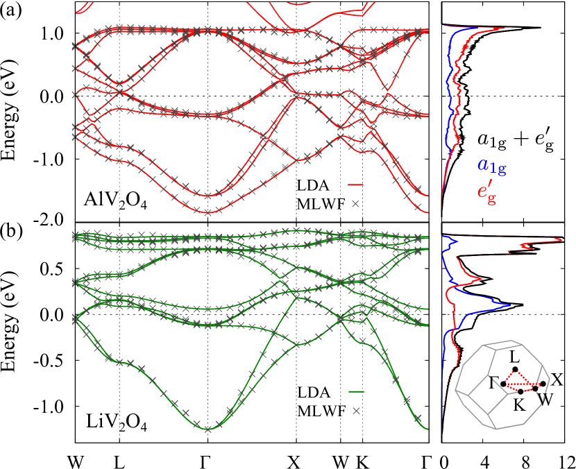
Figure 1: (color online). Electronic states for (a) AlV₂O₄ and (b) LiV₂O₄. The Fermi level is set to zero. In the left panels, the curves denote the band structures obtained by the relativistic LDA calculations, while the results of the MLWF fitting are shown by the crosses. The right panels represent the DOS calculated by the MLWFs. The results decomposed into the $a_{\rm 1g}$ and $e^{\prime}_{\rm g}$ components are also shown. The inset in the right panel of (b) represents the first Brillouin zone for the pyrochlore lattice structure composed of V cations.

The density of states (DOS) is shown in the right panels of Fig. 1. The results for AlV₂O₄ and LiV₂O₄ show contrasting behavior. In AlV₂O₄, the DOS is featureless near the Fermi level, and the $a_{\rm 1g}$ and two $e^{\prime}_{\rm g}$ orbitals are almost equally occupied. On the other hand, in LiV₂O₄, the DOS near the Fermi level strongly depends on the energy, which is dominated by the $a_{\rm 1g}$ component. The difference of the DOS mainly comes from the difference in the transfer integrals.

III.1.2 Tight-binding parameter

Tables 1 and 2 show the transfer integrals $t_{\zeta,\zeta^{\prime}}$ calculated by the MLWFs. For both compounds, the nearest-neighbor transfer is larger than that of the second and third neighbors. It is also common that the most dominant transfer is the $dd\sigma$ component between nearest-neighbor sites, which is schematically shown in Fig. 2. However, the ratio of the diagonal $dd\sigma$ component to the off-diagonal ones is largely different between the two compounds: the $dd\sigma$ transfer is more than 30 times as large as the off-diagonal $d_{xy}$-$d_{yz}$ one in AlV₂O₄, whereas it is about twice of the $d_{zx}$-$d_{yz}$ one in LiV₂O₄.

Table 1: Transfer integrals $t_{\zeta,\zeta^{\prime}}[\bm{\delta}]$ obtained from the MLWF analysis for AlV₂O₄ between (a) nearest-neighbor, (b) second-neighbor, and (c) third-neighbor sites in the basis of ($d_{xy},d_{yz},d_{zx}$). (d) represents the nearest-neighbor transfer integrals in the basis of ($a_{\rm 1g},e^{\prime}_{\rm g,1},e^{\prime}_{\rm g,2}$). The displacement vector $\bm{\delta}$ is ($a/4,a/4,0$), ($a/2,a/4,-a/4$), ($a/2,a/2,0$), ($a/4,a/4,0$) for (a), (b), (c), and (d), respectively. $a$ is the lattice constant for the cubic unit cell of the pyrochlore lattice. The unit is meV. The values less than 1 meV are omitted.

(a)	$d_{xy}$	$d_{yz}$	$d_{zx}$
$d_{xy}$	-467	15	15
$d_{yz}$	-15	132	2
$d_{zx}$	-15	2	132

(b)	$d_{xy}$	$d_{yz}$	$d_{zx}$
$d_{xy}$	14	2	-9
$d_{yz}$	-2	4	-2
$d_{zx}$	11	2	14

(c)	$d_{xy}$	$d_{yz}$	$d_{zx}$
$d_{xy}$	-	2	2
$d_{yz}$	2	-	8
$d_{zx}$	2	8	-

(d)	$a_{\rm 1g}$	$e^{\prime}_{\rm g,1}$	$e^{\prime}_{\rm g,2}$
$a_{\rm 1g}$	-66	215	215
$e^{\prime}_{\rm g,1}$	-185	266	0
$e^{\prime}_{\rm g,2}$	-185	0	-130

Table 2: Transfer integrals for LiV₂O₄. The notations are the same as in Table 1.

(a)	$d_{xy}$	$d_{yz}$	$d_{zx}$
$d_{xy}$	-223	-45	-45
$d_{yz}$	45	91	-112
$d_{zx}$	45	-112	91

(b)	$d_{xy}$	$d_{yz}$	$d_{zx}$
$d_{xy}$	10	7	4
$d_{yz}$	-3	1	-7
$d_{zx}$	-2	3	10

(c)	$d_{xy}$	$d_{yz}$	$d_{zx}$
$d_{xy}$	-56	-	-
$d_{yz}$	-	-	5
$d_{zx}$	-	5	-

(d)	$a_{\rm 1g}$	$e^{\prime}_{\rm g,1}$	$e^{\prime}_{\rm g,2}$
$a_{\rm 1g}$	-88	22	22
$e^{\prime}_{\rm g,1}$	-112	156	0
$e^{\prime}_{\rm g,2}$	-112	0	-202

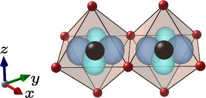
Figure 2: (color online). Schematic picture of edge-sharing VO₆ octahedra. The black and red spheres denote V and O, respectively. A pair of $d_{xy}$ orbitals is drawn to show the $dd\sigma$ overlap.

The difference of the transfer integrals between the two compounds is also seen in the ($a_{\rm 1g}$, $e^{\prime}_{\rm g}$) representation. For AlV₂O₄, as shown in Table 1(d), both of the off-diagonal components are nearly three times as large as the diagonal $a_{\rm 1g}$-$a_{\rm 1g}$ one in magnitude, and comparable to the diagonal $e^{\prime}_{\rm g}$-$e^{\prime}_{\rm g}$ ones. In contrast, for LiV₂O₄, the diagonal $e^{\prime}_{\rm g}$-$e^{\prime}_{\rm g}$ components are dominant, as shown in Table 2(d). The quantitative difference plays a decisive role in the contrasting behavior between the two compounds, as detailed below.

Unlike the transfer integrals, the coupling constants of the one-body on-site terms are almost the same for the two compounds. For AlV₂O₄ and LiV₂O₄, we obtain the estimates the trigonal crystal field splitting $\Delta_{\rm trig}=53$ meV and 61 meV, respectively, while spin-orbit coupling $\lambda_{\rm SOI}=26$ meV and 27 meV, respectively.

III.2 Generalized Susceptibility and Eigenmode Analysis

To study the fluctuations of AlV₂O₄ and LiV₂O₄, generalized susceptibility is calculated. After the computation of the static bare susceptibility, electron correlation is included at the level of RPA. By the eigenmode analysis of the generalized susceptibility, charge, spin, and orbital fluctuations are obtained.

III.2.1 Bare susceptibility

Based on the non-interacting Hamiltonian constructed from the MLWFs, we first calculate the static bare susceptibility $\chi^{(0)}_{\alpha\beta\rho;\alpha^{\prime}\beta^{\prime}\rho^{\prime}}(\bm{q})$. The matrix size is $144\times 144$: four sublattices (only diagonal) with three orbital and two spin components [$4\times(3\times 2)^{2}=144$]. In the calculations, we replace the integral of $\bm{k}$ over the first Brillouin zone by the summation for $32^{3}$ $\bm{k}$ grid points, while we take the summation of $\omega_{k}$ analytically.

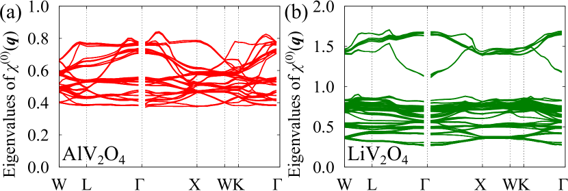
Figure 3: (color online). Eigenvalues of $\chi^{(0)}(\bm{q})$ calculated by using the tight-binding parameters estimated by the MLWFs for (a) AlV₂O₄ and (b) LiV₂O₄. The calculations are done at $T=10$ K.

Figure 3 shows all the eigenvalues of $\chi^{(0)}(\bm{q})$ for AlV₂O₄ and LiV₂O₄. The results look very differently: the eigenmodes are rather entangled in the entire spectrum for AlV₂O₄, whereas the result for LiV₂O₄ shows sixteen eigenmodes well separated from the other modes. Analyzing the eigenvectors of the sixteen eigenmodes, we find that they are dominantly in the $a_{\rm 1g}$ orbital sector, which is anticipated from the DOS in Fig. 1(b).

III.2.2 RPA calculation and eigenmode analysis of AlV₂O₄

Next, we calculate the generalized susceptibility by including the effect of electron correlations in a perturbative way at the level of RPA. First, let us discuss the results for AlV₂O₄. We investigate the generalized susceptibility obtained by RPA, $\chi^{\rm RPA}$, while changing $U$, $J_{\rm H}$, and $V$. Among the parameters, we find that $V$ induces particularly interesting behavior, which might be related with the heptamer formation in AlV₂O₄, as discussed below.

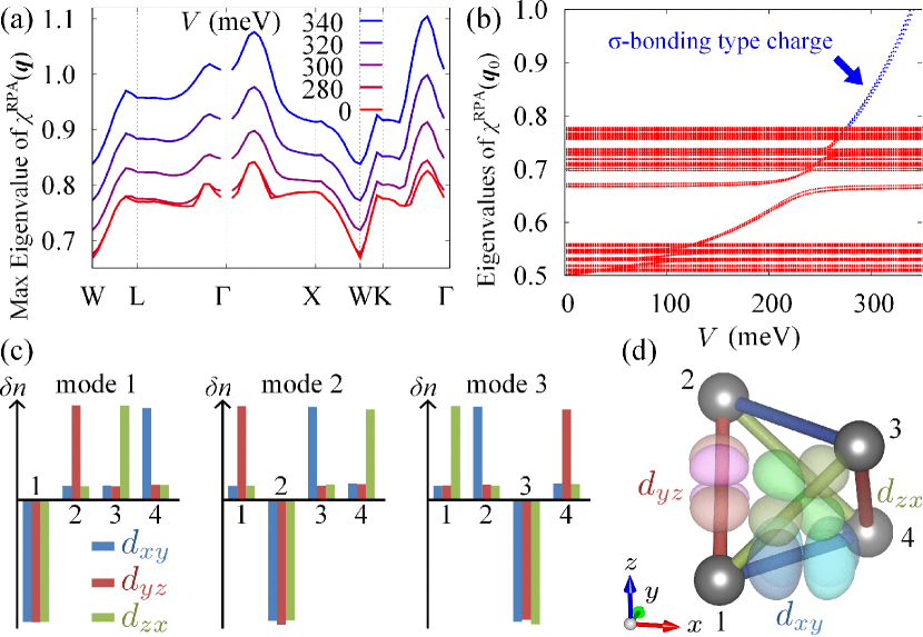
Figure 4: (color online). (a) $V$ dependence of the maximum eigenvalues of $\chi^{\rm RPA}(\bm{q})$ for AlV₂O₄. (b) $V$ dependence of the eigenvalues at $\bm{q}_{0}=(\pi/16,\pi/16,\pi/16)$, which is the smallest wave number along the $\Gamma$-L line in the present calculations. In (a) and (b), we take $U=300$ meV and $J_{\rm H}=30$ meV, while the other parameters are the same as in Fig. 3(a). (c) $\sigma$-bonding type charge fluctuations obtained from the eigenmode analysis. The vertical axis represents the fluctuation of the electron density in arbitrary units. The histogram represents the density fluctuations decomposed into the $d_{xy}$, $d_{yz}$, and $d_{zx}$ orbitals. The numbers 1-4 in the horizontal axis denote the sublattices. (d) Schematic visualization of the fluctuations in the mode 1 in (a).

Figure 4(a) shows the largest eigenvalues of $\chi^{\rm RPA}$, which are considerably enhanced by increasing $V$. As shown in Fig. 4(b), the enhancement occurs in particular eigenmodes, whereas all the other modes are almost insensitive to $V$. To clarify the nature of these enhanced fluctuations by $V$, we analyze the eigenvectors of the three quasi-degenerate modes Uehara et al. . We find that the dominant fluctuations are in the charge sector. Figure 4(c) shows the fluctuations of local electron densities. In all the three modes, the density fluctuation at one sublattice has the opposite sign to the other three, and the net density fluctuation vanishes in the four-site tetrahedron. Note that, while the densities at the sublattices 1, 2, and 3 are suppressed in the modes 1, 2, and 3, respectively, one can make the mode 4 in which the sublattice 4 is suppressed by a linear combination of the modes 1-3.

Interestingly, we find that the density fluctuations in these modes are strongly orbital dependent, as shown in Fig. 4(c). The orbital dependence indicates that the dominant fluctuations occur through the $dd\sigma$ orbital on each bond. For instance, in the mode 1, the charge density in the $d_{yz}$ orbital is dominantly transferred between the sites 1 and 2 on the $yz$ plane, which is regarded as the charge fluctuation through the $dd\sigma$ orbital. The bond- and orbital-dependent fluctuations are schematically shown in Fig. 4(d). Thus, the fluctuations of the three modes sensitive to $V$ are of $\sigma$-bonding type. The importance of such $\sigma$-bonding states in the heptamer was suggested in the previous experimental and theoretical studies Horibe et al. (2006); Matsuda et al. (2006). Hence, our results for the dominant charge fluctuations in $\sigma$-bonding orbitals suggest that the inter-site Coulomb repulsion plays a role in the self-organization of heptamers in AlV₂O₄.

We note that the values of $V$ in the present RPA calculations are rather large: in reality, the bare value of $V$ will be considerably smaller than $U$. Nevertheless, our finding might be relevant to the heptamer formation in AlV₂O₄ due to the following reason. The structural change associated with the heptamer formation clearly indicates the importance of the Peierls-type electron-phonon coupling. Such inter-site phonons are known to give rise to an effective repulsive interaction for electrons: indeed, the integration of phonon degrees of freedom leaves the effective $V$ term, together with other inter-site interactions Heeger et al. (1988). We regard that such effects are included in the value of $V$ in the RPA analysis, although the realistic estimate is left for future study.

III.2.3 RPA calculation and eigenmode analysis of LiV₂O₄

Next, we discuss the results of $\chi^{\rm RPA}$ for LiV₂O₄. We here focus on the effect of $U$, while $V$ leads to a different charge fluctuation from AlV₂O₄ as mentioned below. Figure 5(a) shows $U$ dependence of the maximum eigenvalues of $\chi^{\rm RPA}$. The maximum eigenvalues are enhanced by $U$ and become more dispersive.

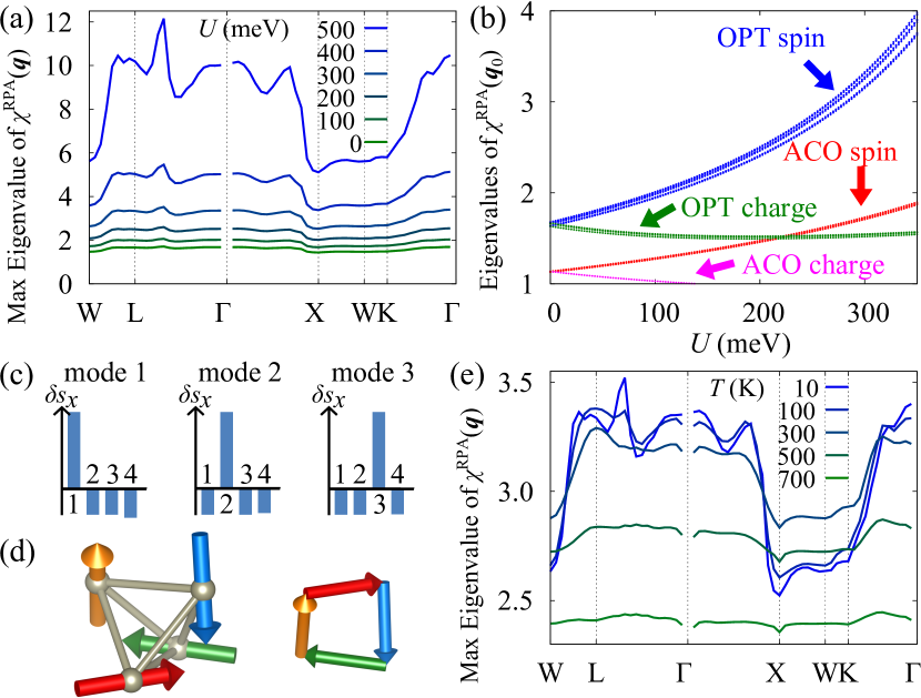
Figure 5: (color online). (a) $U$ dependence of the maximum eigenvalues of $\chi^{\rm RPA}(\bm{q})$ for LiV₂O₄. (b) $U$ dependence of the largest sixteen eigenvalues at $\bm{q}_{0}$. OPT (ACO) represents optical (acoustic: uniform in the unit cell) type fluctuation. In (a) and (b), the calculations are done at $J_{\rm H}/U=0.1$ and $V=0$, while the other parameters are taken to be the same as in Fig. 3(b). (c) OPT spin fluctuations obtained from the eigenmode analysis. The vertical axis represents the spin fluctuations of the $x$ component in arbitrary units. The other components are qualitatively similar. (d) Schematic visualization of the OPT spin fluctuations, in which the net spin fluctuation vanishes in the four-site tetrahedron. (e) $T$ dependence of the maximum eigenvalues of $\chi^{\rm RPA}(\bm{q})$ at $U=300$ meV, $J_{\rm H}=30$ meV, and $V=0$.

We plot $U$ dependence of the largest sixteen eigenvalues of $\chi^{\rm RPA}$ in Fig. 5(b). Note that all of them are of $a_{\rm 1g}$ character as discussed above. We find that nine eigenmodes are largely enhanced by $U$. We also elucidate that all the nine eigenmodes consist of spin fluctuations. Figure 5(c) shows the three of them, which are the spin fluctuations in the $x$ component. In all the three modes, the spin fluctuation $\delta s^{x}$ at one sublattice has an opposite sign to the other three; the net $\delta s^{x}$ vanishes in the four-site tetrahedron. Similar situations are found also in the $y$ and $z$ components. Namely, the spin fluctuations satisfy the relation $\sum_{\rho=1}^{4}\delta\bm{s}_{\rho}=0$, where $\delta\bm{s}_{\rho}=(\delta s_{\rho}^{x},\delta s_{\rho}^{y},\delta s_{\rho}^{z})$. Hence, we call them the optical-type spin fluctuations, whose schematic visualization is shown in Fig. 5(d). As the zero-sum condition is often met in frustrated spin systems, our results suggest that the dominant fluctuations in LiV₂O₄ appear in the $a_{\rm 1g}$ spins under strong geometrical frustration.

On the other hand, we find that $V$ enhances a charge fluctuation in the $a_{\rm 1g}$ orbital, where the net $a_{\rm 1g}$ density fluctuation vanishes in the four-site tetrahedron (not shown here). The result is in sharp contrast to the case of AlV₂O₄, in which $\sigma$-type fluctuation is enhanced by $V$.

Figure 5(e) shows $T$ dependence of the maximum eigenvalues of $\chi^{\rm RPA}$ for LiV₂O₄. The dominant instability is always in the optical-type spin fluctuations in the $a_{\rm 1g}$ orbital. Although the mode is almost $\bm{q}$ independent at high $T\gtrsim 500$ K, it develops the $\bm{q}$ dependence below $\sim 300$ K. At lower $T$ below 100 K, the peak between the $\Gamma$-L line develops, being the dominant instability. We note that a similar peak appeared in the previous theoretical study Yushankhai et al. (2007), while the model and the RPA treatment were different from ours. The growth of the incommensurate peak is potentially related with that observed in the inelastic neutron scattering for LiV₂O₄ below 80 K Lee et al. (2001); Tomiyasu et al. (2014). Nevertheless, further studies beyond the current weak-coupling approach are necessary to address the heavy fermion behavior, as the recent NMR experiment suggests local moments in the $a_{\rm 1g}$ orbital even at high $T$ Shimizu et al. (2012).

IV Discussion

It is worth noting that the electronic structure obtained by LDA and MLWF analyses plays an important role in the dominant fluctuations enhanced by electron correlations. In AlV₂O₄, three $t_{\rm 2g}$ orbitals almost equally contribute to the DOS near the Fermi level as shown in Fig. 1(a), and furthermore, the $dd\sigma$ components in the transfer integrals are dominant as shown in Table 1. These are directly reflected in the dominant $\sigma$-type charge fluctuation in Fig. 4. On the other hand, in LiV₂O₄, the diagonal components represented in the ($a_{\rm 1g}$, $e^{\prime}_{\rm g}$) basis dominate the transfer integrals, as shown in Table 2(d). This is closely related with the dominant $a_{\rm 1g}$ spin fluctuation in Fig. 5. Thus, for both compounds, the orbital channel for the dominant fluctuations are deduced from the transfer integrals composed from the LDA band structures, although the actual types of fluctuations are clarified only after performing RPA.

Finally, we discuss the pressure effect on LiV₂O₄ in the present scheme. We performed the LDA calculation by reducing the lattice constant by $2$% from the original value, which approximately corresponds to the situation at the pressure 6.3 GPa Takeda et al. (2005). By the energy optimization with respect to the $u$ parameter, which controls the trigonal distortion, we find that the value of $u$ decreases from 0.262 to 0.259. Although it approaches that for AlV₂O₄ ($u=0.251$) Katsufuji , the $a_{\rm 1g}$ component remains dominant in the DOS. Accordingly, our calculations for the generalized susceptibility indicate that the dominant instability is still in the $a_{\rm 1g}$ optical-type spin fluctuations and does not qualitatively change from ambient pressure. The results imply that the pressure-induced metal-insulator transition in LiV₂O₄ is caused by a different mechanism from the cluster formation in AlV₂O₄, and hence, the associated structural change is also likely to be different from AlV₂O₄.

V Summary

In summary, for a systematic understanding of the contrasting behavior in two mixed valence spinels, AlV₂O₄ and LiV₂O₄, we have analyzed charge-spin-orbital fluctuations in the multiband Hubbard models, whose one-body part is constructed by LDA calculations and MLWF analysis. From the eigenmode analysis of the generalized susceptibility obtained by RPA, we found that, in AlV₂O₄, the $\sigma$-bonding type charge-orbital fluctuations are enhanced by the intersite repulsion, which provides a clue for understanding of the seven-site cluster formation. In contrast, for LiV₂O₄, the optical-type spin fluctuation in the $a_{\rm 1g}$ orbital is strongly enhanced by $U$ at an incommensurate wave number at low temperatures. We also discussed the pressure effect on LiV₂O₄ and deduced that the mechanism of pressure-induced metal-insulator transition might be different from the cluster formation in AlV₂O₄.

As the present analysis is based on the LDA band structures and the electron correlations are included at the level of RPA, it is difficult to discuss the strong correlation effects, for instance, the large mass enhancement at low temperature in LiV₂O₄. It is necessary to adopt more sophisticated methods that can treat the renormalization of the band structures and occupations of each orbitals. This is left for future study.

References

- Tokura and Nagaosa (2000) Y. Tokura and N. Nagaosa, Science 288, 462 (2000).
- Lacroix et al. (2011) C. Lacroix, P. Mendels, and F. Mila, Introduction to Frustrated Magnetism (Springer, London, 2011).
- Lee et al. (2010) S.-H. Lee, H. Takagi, D. Louca, M. Matsuda, S. Ji, H. Ueda, Y. Ueda, T. Katsufuji, J.-H. Chung, S. Park, et al., J. Phys. Soc. Jpn. 79, 011004 (2010).
- Matsuno et al. (2001) K. Matsuno, T. Katsufuji, S. Mori, Y. Moritomo, A. Machida, E. Nishibori, M. Takata, M. Sakata, N. Yamamoto, and H. Takagi, J. Phys. Soc. Jpn. 70, 1456 (2001).
- Horibe et al. (2006) Y. Horibe, M. Shingu, K. Kurushima, H. Ishibashi, N. Ikeda, K. Kato, Y. Motome, N. Furukawa, S. Mori, and T. Katsufuji, Phys. Rev. Lett. 96, 086406 (2006).
- Matsuda et al. (2006) K. Matsuda, N. Furukawa, and Y. Motome, J. Phys. Soc. Jpn. 75, 124716 (2006).
- Rogers et al. (1967) D. B. Rogers, J. L. Gillson, and T. E. Gier, Solid State. Commun. 263, 5 (1967).
- Kondo et al. (1997) S. Kondo, D. C. Johnston, C. A. Swenson, F. Borsa, A. V. Mahajan, L. L. Miller, T. Gu, A. I. Goldman, M. B. Maple, D. A. Gajewski, et al., Phys. Rev. Lett. 78, 3729 (1997).
- Urano et al. (2000) C. Urano, M. Nohara, S. Kondo, F. Sakai, H. Takagi, T. Shiraki, and T. Okubo, Phys. Rev. Lett. 85, 1052 (2000).
- Anisimov et al. (1999) V. I. Anisimov, M. A. Korotin, M. Zölfl, T. Pruschke, K. Le Hur, and T. M. Rice, Phys. Rev. Lett. 83, 364 (1999).
- Eyert et al. (1999) V. Eyert, K.-H. Hock, S. Horn, A. Loidl, and P. S. Riseborough, Europhys. Lett. 46, 762 (1999).
- Kusunose et al. (2000) H. Kusunose, S. Yotsuhashi, and K. Miyake, Phys. Rev. B 62, 4403 (2000).
- Tsunetsugu (2002) H. Tsunetsugu, J. Phys. Soc. Jpn. 71, 1844 (2002).
- Yamashita and Ueda (2003) Y. Yamashita and K. Ueda, Phys. Rev. B 67, 195107 (2003).
- Arita et al. (2007) R. Arita, K. Held, A. V. Lukoyanov, and V. I. Anisimov, Phys. Rev. Lett. 98, 166402 (2007).
- Yushankhai et al. (2007) V. Yushankhai, A. Yaresko, P. Fulde, and P. Thalmeier, Phys. Rev. B 76, 085111 (2007).
- Hattori and Tsunetsugu (2009) K. Hattori and H. Tsunetsugu, Phys. Rev. B 79, 035115 (2009).
- Urano (2000) C. Urano, Ph.D. thesis, The University of Tokyo (2000).
- Takeda et al. (2005) K. Takeda, H. Hidaka, H. Kotegawa, T. Kobayashi, K. Shimizu, H. Harima, K. Fujiwara, K. Miyoshi, J. Takeuchi, Y. Ohishi, et al., Physica B Condens. Matter 359-361, 1312 (2005).
- Irizawa et al. (2011) A. Irizawa, S. Suga, G. Isoyama, K. Shimai, K. Sato, K. Iizuka, T. Nanba, A. Higashiya, S. Niitaka, and H. Takagi, Phys. Rev. B 84, 235116 (2011).
- Pinsard-Gaudart et al. (2007) L. Pinsard-Gaudart, N. Dragoe, P. Lagarde, A. M. Flank, J. P. Itie, A. Congeduti, P. Roy, S. Niitaka, and H. Takagi, Phys. Rev. B 76, 045119 (2007).
- Hohenberg and Kohn (1964) P. Hohenberg and W. Kohn, Phys. Rev. 136, B864 (1964).
- Kohn and Sham (1965) W. Kohn and L. J. Sham, Phys. Rev. 140, A1133 (1965).
- (24) http://qmas.jp/.
- Shinaoka et al. (2012) H. Shinaoka, T. Miyake, and S. Ishibashi, Phys. Rev. Lett. 108, 247204 (2012).
- (26) A. Uehara, H. Shinaoka, and Y. Motome, preprint (arXiv:1506.06231).
- Karolak et al. (2010) M. Karolak, G. Ulm, T. Wehling, V. Mazurenko, A. Poteryaev, and A. Lichtenstein, J. Elect. Spectr. 181, 11 (2010).
- (28) T. Katsufuji, private communication.
- Chmaissem et al. (1997) O. Chmaissem, J. D. Jorgensen, S. Kondo, and D. C. Johnston, Phys. Rev. Lett. 79, 4866 (1997).
- Matsuno et al. (2000) J. Matsuno, K. Kobayashi, A. Fujimori, L. Mattheiss, and Y. Ueda, Physica B Condens. Matter 281-282, 28 (2000).
- Marzari and Vanderbilt (1997) N. Marzari and D. Vanderbilt, Phys. Rev. B 56, 12847 (1997).
- Souza et al. (2001) I. Souza, N. Marzari, and D. Vanderbilt, Phys. Rev. B 65, 035109 (2001).
- Heeger et al. (1988) A. J. Heeger, S. Kivelson, J. R. Schrieffer, and W. P. Su, Rev. Mod. Phys. 60, 781 (1988).
- Lee et al. (2001) S.-H. Lee, Y. Qiu, C. Broholm, Y. Ueda, and J. J. Rush, Phys. Rev. Lett. 86, 5554 (2001).
- Tomiyasu et al. (2014) K. Tomiyasu, K. Iwasa, H. Ueda, S. Niitaka, H. Takagi, S. Ohira-Kawamura, T. Kikuchi, Y. Inamura, K. Nakajima, and K. Yamada, Phys. Rev. Lett. 113, 236402 (2014).
- Shimizu et al. (2012) Y. Shimizu, H. Takeda, M. Itoh, S. Niitaka, and H. Takagi, Nat. Commun. 3, 981 (2012).
- Momma and Izumi (2011) K. Momma and F. Izumi, J. Appl. Crystallogr 44, 1272 (2011).