On enforcing maximum principles and
achieving element-wise species balance for
advection-diffusion-reaction equations under
the finite element method
   
Authored by
M. K. Mudunuru

Graduate Student, University of Houston.
K. B. Nakshatrala

Department of Civil & Environmental Engineering
University of Houston, Houston, Texas 77204–4003.
phone: +1-713-743-4418, e-mail: knakshatrala@uh.edu
website: http://www.cive.uh.edu/faculty/nakshatrala

These figures show the fate of the product in a transient transport-controlled bimolecular reaction under vortex-stirred mixing. The left figure is obtained using a popular numerical formulation, which violates the non-negative constraint. The right figure is based on the proposed computational framework. These figures clearly illustrate the main contribution of this paper: The proposed computational framework produces physically meaningful results for advective-diffusive-reactive systems, which is not the case with many popular formulations.

Abstract.

We present a robust computational framework for advective-diffusive-reactive systems that satisfies maximum principles, the non-negative constraint, and element-wise species balance property. The proposed methodology is valid on general computational grids, can handle heterogeneous anisotropic media, and provides accurate numerical solutions even for very high Péclet numbers. The significant contribution of this paper is to incorporate advection (which makes the spatial part of the differential operator non-self-adjoint) into the non-negative computational framework, and overcome numerical challenges associated with advection. We employ low-order mixed finite element formulations based on least-squares formalism, and enforce explicit constraints on the discrete problem to meet the desired properties. The resulting constrained discrete problem belongs to convex quadratic programming for which a unique solution exists. Maximum principles and the non-negative constraint give rise to bound constraints while element-wise species balance gives rise to equality constraints. The resulting convex quadratic programming problems are solved using an interior-point algorithm. Several numerical results pertaining to advection-dominated problems are presented to illustrate the robustness, convergence, and the overall performance of the proposed computational framework.

1. INTRODUCTION AND MOTIVATION

Advection-diffusion-reaction (ADR) equations are pervasive in the mathematical modeling of several important phenomena in mathematical physics and engineering sciences. Some examples include degradation/healing of materials under extreme environmental conditions [1], coupled chemo-thermo-mechano-diffusion problems in composites [2], contaminant transport [3], turbulent mixing in atmospheric sciences [4], diffusion-controlled biochemical reactions [5], tracer modeling in hydrogeology [6], and ionic mobility in biological systems [7]. Additionally, ADR equation serves as a good mathematical model in numerical analysis, as it offers various unique challenges in obtaining stable and accurate numerical solutions [8].

The primary variables in these mathematical models are typically the concentration and/or the (absolute) temperature. These quantities naturally attain non-negative values. Under some popular constitutive models (such as Fourier model and Fickian model, and their generalizations), these physical quantities satisfy diffusion-type equations, which are elliptic/parabolic partial differential equations (PDEs) and can be non-self-adjoint. These PDEs are known to satisfy important mathematical properties like maximum principles and the non-negative constraint (e.g., see [9]). A predictive numerical formulation needs to satisfy these mathematical properties and physical laws like the (local and global) species balance. It is well-documented in the literature that traditional numerical methods perform poorly for advection-dominated ADR equations (e.g., see [10, 8]). In the past few decades, considerable progress has been made to obtain sufficiently accurate numerical solutions for ADR equations on coarse computational grids [11]. It is then natural to ask: “why there is a need for yet another numerical formulation for ADR equation?”. We now outline several reasons for such a need.

1. Localized phenomena and node-to-node spurious oscillations: For advection-dominated problems, it is well-known that the standard single-field Galerkin finite element formulation gives node-to-node spurious oscillations on coarse computational grids [8]. Moreover, it cannot capture steep gradients such as interior and boundary layers. Various alternate numerical techniques have been proposed to avoid these spurious oscillations [12]. Some methods seem to capture steep gradients in interior layers while others capture boundary layers. However, most of them do not seem to capture both interior and boundary layers, and at the same time avoid node-to-node spurious oscillations [13]. A notable work towards this direction is by Hsieh and Yang [14], which can capture both interior and boundary layers under adequate mesh refinement. However, this formulation has several other deficiencies some of which are discussed below and illustrated using numerical examples in subsequent sections.

2. Violation of the non-negative constraint and maximum principles: As mentioned earlier, physical quantities such as concentration and temperature naturally attain non-negative values. It is highly desirable for a numerical formulation to respect these physical constraints. This is particularly important in a numerical simulation of reactive transport, as a negative value for concentration will result in an algorithmic failure. However, it is clearly documented in the literature that many existing formulations based on finite element [15, 16, 17], finite volume [18], and finite difference [19] do not satisfy the non-negative constraint and maximum principles in the discrete setting. They also discuss various methodologies to satisfy such properties. But most of these methodologies are for pure diffusion equations, which are self-adjoint. For example, in Reference [16], two mixed formulations based on RT0 spaces and variational multiscale formalism have been modified to meet the non-negative constraint for diffusion equations. This approach is not directly applicable to ADR equations for two reasons. First, these formulations do not cure the node-to-node spurious oscillations. Second, they do not possess a variational structure for ADR equations. Some numerical formulations are constructed to satisfy the non-negative constraint and maximum principles by taking advection into account (e.g., [20, 21]). However, they do not satisfy local and global species balance, and are restricted to isotropic diffusion. Conservative post-processing methods exist in the literature to recover certain desired properties such as species balance. But such formulations are not variationally consistent [22].

3. Satisfying local and global species balance: In transport problems, the balance of species is an important physical law that needs to be met. It is therefore desirable for a numerical formulation to satisfy local and global species balance, say, up to machine precision (which is approximately $10^{-16}$ on a 64-bit machine). However, many finite element formulations do not satisfy local and global species balance (see [23, 11, 14]). The main focus of the methods outlined in these papers is to capture the localized phenomena such as boundary and interior layers. Moreover, these works did not quantify the errors incurred in satisfying local species balance and global species balance. It needs to be emphasized that many finite element methods do exist that inherently satisfy local and global species balance, for example, Raviart-Thomas spaces [24] and BDM spaces [25]. But these approaches do not fix other issues discussed herein such as the node-to-node spurious oscillations or meeting maximum principles for ADR equations.

4. Other influential factors: Some other important factors that can affect the performance of a numerical formulation are the advection velocity field and its divergence, anisotropy of the medium, reaction coefficients, topology of the medium, computational mesh, multiple spatial-scales arising due to the heterogeneity of the medium, and multiple time-scales involved in various physical processes. Another aspect that brings tremendous numerical challenges is chemical reactions involving multiple species.

It is a herculean task to address all the aforementioned deficiencies, and we strongly believe that it may take a series of papers to overcome all the deficiencies. A similar sentiment is shared in the review article by Stynes entitled “Numerical methods for convection-diffusion problems or the 30 years war” [26]. We therefore take motivation from George Pólya’s quote [27]: “If you can’t solve a problem, then there is an easier problem you can solve: find it.” In this paper, we shall pose a problem that is simpler than the grand challenge of overcoming all the aforementioned numerical deficiencies but still make a significant advancement with respect to the current state-of-the-art. We then provide a solution to this simpler problem. To state it more precisely, the main contribution of this paper is developing a least-squares-based finite element framework for ADR equations that possesses the following properties on general computational grids:

1. No spurious node-to-node oscillations in the entire domain.

2. Captures interior and boundary layers for advection-dominated problems.

3. Satisfies discrete maximum principles and the non-negative constraint.

4. Satisfies local and global species balance.

5. Gives sufficiently accurate solutions even on coarse computational grids.

To the best of authors’ knowledge, there exists no finite element methodology for advective-diffusive-reactive systems that possesses the desirable properties (P1)–(P5).

The rest of the paper is organized as follows. Section 2 presents the governing equations for an advective-diffusive-reactive system, and discusses the associated mathematical properties. Section 3 outlines several plausible approaches, and discusses their drawbacks in meeting the mentioned mathematical properties. In Section 4, we propose a constrained optimization-based low-order mixed finite element method to satisfy maximum principles, the non-negative constraint, local species balance, and global species balance. In Section 5, we perform a numerical $h$-convergence study using a benchmark problem. In Section 6, we specialize to transport-limited bimolecular reactions to solve problems related to plume development and mixing in isotropic/anisotropic heterogeneous media. Finally, conclusions are drawn in Section 7. If one is interested only in the implementation of the proposed method, the reader can directly go to Section 4, and appendices A and C.

We shall denote scalars by lowercase English alphabet or lowercase Greek alphabet (e.g., concentration $c$ and stabilization parameter $\tau$). The continuum vectors are denoted by lowercase boldface normal letters, and the second-order tensors will be denoted using uppercase boldface normal letters (e.g., vector $\mathbf{x}$ and second-order tensor $\mathbf{D}$). In the finite element context, the vectors are denoted using lowercase boldface italic letters, and the matrices are denoted using uppercase boldface italic letters (e.g., vector $\boldsymbol{v}$ and matrix $\boldsymbol{K}$). We shall use NN to denote non-negative, DMP denotes discrete maximum principle, LSB to denote local species balance, and GSB to denote global species balance. We shall use XSeed to denote the number of (finite element) nodes in a mesh along x-direction. Likewise for YSeed. Other notational conventions adopted in this paper are introduced as needed.

2. GOVERNING EQUATIONS: ADVECTIVE-DIFFUSIVE-REACTIVE SYSTEMS

Let $\Omega\subset\mathbb{R}^{nd}$ be a bounded open domain, where “$nd$” denotes the number of spatial dimensions. The boundary of the domain is denoted by $\partial\Omega$, which is assumed to be piecewise smooth. Mathematically, $\partial\Omega:=\overline{\Omega}-\Omega$, where a superposed bar denotes the set closure. A spatial point is denoted by $\mathbf{x}\in\overline{\Omega}$. The gradient and divergence operators with respect to $\mathbf{x}$ are, respectively, denoted by $\mathrm{grad}[\bullet]$ and $\mathrm{div}[\bullet]$. The unit outward normal to the boundary is denoted by $\widehat{\mathbf{n}}(\mathbf{x})$. Let $c(\mathbf{x})$ denote the concentration field. The boundary is divided into two parts: $\Gamma^{c}$ and $\Gamma^{q}$ such that $\mathrm{meas}(\Gamma^{c})>0$, $\overline{\Gamma}^{c}\cup\overline{\Gamma}^{q}=\partial\Omega$, and $\Gamma^{c}\cap\Gamma^{q}=\emptyset$. $\Gamma^{c}$ is the part of the boundary on which the concentration is prescribed and $\Gamma^{q}$ is the other part of the boundary on which the diffusive/total flux is prescribed.

The governing equations for steady-state response of an ADR system take the following form:

$$\alpha(\mathbf{x})c(\mathbf{x})+\mathrm{div}\left[c(\mathbf{x})\mathbf{v}(\mathbf{x})-\mathbf{D}(\mathbf{x})\mathrm{grad}[c(\mathbf{x})]\right]=f(\mathbf{x})\quad \mathrm{in}\;\Omega$$ (2.1a)

$$c(\mathbf{x})=c^{\mathrm{p}}(\mathbf{x})\quad \mathrm{on}\;\Gamma^{c}$$ (2.1b)

$$\left(\left(\frac{1-\mathrm{Sign}[\mathbf{v}\bullet\widehat{\mathbf{n}}]}{2}\right)\mathbf{v}(\mathbf{x})c(\mathbf{x})-\mathbf{D}(\mathbf{x})\mathrm{grad}[c(\mathbf{x})]\right)\bullet\widehat{\mathbf{n}}(\mathbf{x})=q^{\mathrm{p}}(\mathbf{x})\quad \mathrm{on}\;\Gamma^{q}$$ (2.1c)

$\mathbf{v}(\mathbf{x})$ is the known advection velocity field, $f(\mathbf{x})$ is the prescribed volumetric source, $\mathbf{D}(\mathbf{x})$ is the anisotropic diffusivity tensor, $\alpha(\mathbf{x})$ is the linear reaction coefficient, $c^{\mathrm{p}}(\mathbf{x})$ is the prescribed concentration, $q^{\mathrm{p}}(\mathbf{x})$ is the prescribed diffusive/total flux, and the sign function is defined as follows:

$$\mathrm{Sign}[\varphi]:=\begin{cases}-1&\quad\mathrm{if}\;\varphi<0\\ 0&\quad\mathrm{if}\;\varphi=0\\ +1&\quad\mathrm{if}\;\varphi>0\end{cases}$$ (2.2)

The advection velocity need not be solenoidal in our treatment (i.e., $\mathrm{div}[\mathbf{v}(\mathbf{x})]$ need not be zero). The Neumann boundary condition given in equation (2.1c) can be interpreted as follows:

$$\widehat{\mathbf{n}}(\mathbf{x})\bullet\left(\mathbf{v}(\mathbf{x})c(\mathbf{x})-\mathbf{D}(\mathbf{x})\mathrm{grad}[c(\mathbf{x})]\right)=q^{\mathrm{p}}(\mathbf{x})\; \mathrm{on}\;\Gamma^{q}_{-}\;(\mbox{total flux on inflow boundary})$$ (2.3a)

$$- \widehat{\mathbf{n}}(\mathbf{x})\bullet\mathbf{D}(\mathbf{x})\mathrm{grad}[c(\mathbf{x})]=q^{\mathrm{p}}(\mathbf{x})\; \mathrm{on}\;\Gamma^{q}_{+}\;(\mbox{diffusive flux on outflow boundary})$$ (2.3b)

where $\Gamma^{q}_{+}$ and $\Gamma^{q}_{-}$ are, respectively, defined as follows (see Figure 1):

$$\Gamma^{q}_{-} :=\left\{\mathbf{x}\in\Gamma^{q}\;\big{|}\;\mathbf{v}(\mathbf{x})\bullet\widehat{\mathbf{n}}(\mathbf{x})<0\right\}\quad (\mathrm{inflow\;boundary})$$ (2.4a)

$$\Gamma^{q}_{+} :=\left\{\mathbf{x}\in\Gamma^{q}\;\big{|}\;\mathbf{v}(\mathbf{x})\bullet\widehat{\mathbf{n}}(\mathbf{x})\geq 0\right\}\quad (\mathrm{outflow\;boundary})$$ (2.4b)

\psfrag{A1}{$\Gamma^{q}_{-}$}\psfrag{A2}{$\Gamma^{c}$}\psfrag{A3}{$\Gamma^{q}_{+}$}\psfrag{v}{$\mathbf{v}(\mathbf{x})$}\psfrag{B1}{P}\psfrag{B2}{Q}\psfrag{B3}{R}\includegraphics[scale={0.75},clip]{Inflow_Outflow_BCs.eps}

Figure 1. This figure illustrates concentration and flux boundary conditions. $\Gamma^{q}_{-}$ corresponds to the inflow boundary while $\Gamma^{q}_{+}$ corresponds to the outflow boundary. Total flux is prescribed on $\Gamma^{q}_{-}$, diffusive flux is prescribed on $\Gamma^{q}_{+}$, and concentration is prescribed on $\Gamma^{c}$. P = $\overline{\Gamma}^{c}\cap\overline{\Gamma}^{q}_{+}$, Q = $\overline{\Gamma}^{c}\cap\overline{\Gamma}^{q}_{-}$, and R = $\overline{\Gamma}^{q}_{+}\cap\overline{\Gamma}^{q}_{-}$. For well-posedness, we have $\overline{\Gamma}^{c}\cup\overline{\Gamma}^{q}_{+}\cup\overline{\Gamma}^{q}_{-}=\partial\Omega$, $\Gamma^{c}\cap\Gamma^{q}_{+}=\emptyset$, $\Gamma^{c}\cap\Gamma^{q}_{-}=\emptyset$, and $\Gamma^{q}_{+}\cap\Gamma^{q}_{-}=\emptyset$.

Remark 2.1.

In the literature, more predominantly in the numerical literature, the term advection is often used synonymously with convection. It should, however, be noted that these two terms describe different physical phenomena, and there is a need to clarify the terminology here. An ADR equation arises from the balance of mass of a given species. In 1D, an ADR equation takes the following form:

$$\alpha(x)c(x)+\frac{d(vc)}{dx}-\frac{d}{dx}\left(D(x)\frac{dc}{dx}\right)=f(x)$$ (2.5)

which is mathematically equivalent to the following equation:

$$\left(\alpha(x)+\frac{dv}{dx}\right)c(x)+v(x)\frac{dc}{dx}-\frac{d}{dx}\left(D(x)\frac{dc}{dx}\right)=f(x)$$ (2.6)

One can obtain a “similar” mathematical equation by linearizing the incompressible Navier-Stokes equation, and an appropriate name for this linearized equation is the convection-dissipation-reaction (CDR) equation. The CDR equation in 1D has the following mathematical form:

$$\frac{dv_{0}}{dx}\tilde{v}(x)+v_{0}(x)\frac{d\tilde{v}}{dx}-\frac{d}{dx}\left(\mu(x)\frac{d\tilde{v}}{dx}\right)=b(x,p_{0}(x))+2v_{0}(x)\frac{dv_{0}}{dx}$$ (2.7)

where $\tilde{v}(x)$ is the velocity of the fluid, and $p_{0}(x)$ and $v_{0}(x)$ are known pressure and velocity fields about which the Navier-Stokes equation is linearized. From equations (2.6) and (2.7), it is evident that 1D ADR equation and 1D CDR equation have similar mathematical forms. However, their physical underpinnings are completely different, as the Navier-Stokes equation is obtained by substituting a specific constitutive model into the balance of linear momentum.

2.1. Weak formulations

The following function spaces will be used in the rest of this paper:

$$\mathcal{C} :=\left\{c(\mathbf{x})\in H^{1}(\Omega)\;\big{|}\;c(\mathbf{x})=c^{\mathrm{p}}(\mathbf{x})\;\mathrm{on}\;\Gamma^{c}\right\}$$ (2.8a)

$$\mathcal{W} :=\left\{w(\mathbf{x})\in H^{1}(\Omega)\;\big{|}\;w(\mathbf{x})=0\;\mathrm{on}\;\Gamma^{c}\right\}$$ (2.8b)

$$\mathcal{Q} :=\left\{\mathbf{q}(\mathbf{x})\in\left(L_{2}(\Omega)\right)^{nd}\;\big{|}\;\mathrm{div}[\mathbf{q}(\mathbf{x})]\in L_{2}(\Omega)\right\}$$ (2.8c)

where $\mathbf{q}(\mathbf{x})=c(\mathbf{x})\mathbf{v}(\mathbf{x})-\mathbf{D}(\mathbf{x})\mathrm{grad}[c(\mathbf{x})]$ and $H^{1}(\Omega)$ is a standard Sobolev space [28]. Given two vector fields $a(\mathbf{x})$ and $b(\mathbf{x})$ on a set $K$, the standard $L_{2}$ inner product over $K$ is denoted as follows:

$$\left(a;b\right)_{K}=\displaystyle\int\limits_{K}a(\mathbf{x})\bullet b(\mathbf{x})\;\mathrm{d}K$$ (2.9)

The subscript will be dropped if $K=\Omega$. The most popular way to construct a weak formulation is to employ the Galerkin formalism. Based on the manner in which one applies the divergence theorem, the single-field Galerkin formulation for equations (2.1a)–(2.1c) can be posed in two different ways.

Single-field Galerkin formulation #1 ($\mathrm{SG}_{1}$): Find $c(\mathbf{x})\in\mathcal{C}$ such that we have

$$(w;\alpha c) -(\mathrm{grad}[w]\bullet\mathbf{v};c)+(\mathrm{grad}[w];\mathbf{D}(\mathbf{x})\mathrm{grad}[c])+\left(w;\left(\frac{1+\mathrm{Sign}[\mathbf{v}\bullet\widehat{\mathbf{n}}]}{2}\right)(\mathbf{v}\bullet\widehat{\mathbf{n}})\;c\right)_{\Gamma^{q}}$$

$$=(w;f)-\left(w;q^{\mathrm{p}}\right)_{\Gamma^{q}}\quad\forall w(\mathbf{x})\in\mathcal{W}$$ (2.10)

Single-field Galerkin formulation #2 ($\mathrm{SG}_{2}$): Find $c(\mathbf{x})\in\mathcal{C}$ such that we have

$$\left(w;\left(\alpha+\mathrm{div}[\mathbf{v}]\right)c\right) +(w;\mathrm{grad}[c]\bullet\mathbf{v})+(\mathrm{grad}[w];\mathbf{D}(\mathbf{x})\mathrm{grad}[c])-\left(w;\left(\frac{1-\mathrm{Sign}[\mathbf{v}\bullet\widehat{\mathbf{n}}]}{2}\right)(\mathbf{v}\bullet\widehat{\mathbf{n}})\;c\right)_{\Gamma^{q}}$$

$$=(w;f)-\left(w;q^{\mathrm{p}}\right)_{\Gamma^{q}}\quad\forall w(\mathbf{x})\in\mathcal{W}$$ (2.11)

Note that the solution obtained will be the same regardless whether we use either $\mathrm{SG}_{1}$ or $\mathrm{SG}_{2}$. However, this is not true if one uses total/diffusive flux on Neumann boundary without giving due consideration to inflow and/or outflow Neumann boundary conditions. For more details, see subsection 2.3.

2.2. Maximum principles and the non-negative constraint

A basic qualitative property of elliptic boundary value problems is the maximum principle. This property gives a priori estimate for $c(\mathbf{x})$ in $\Omega$ through its values on $\Gamma^{c}$. The following assumptions will be made to present a continuous maximum principle for ADR equations with both Dirichlet and Neumann boundary conditions:

1. $\Omega$ is piecewise smooth domain with Lipschitz continuous boundary $\partial\Omega$.

2. The scalar functions $\alpha:\overline{\Omega}\rightarrow\mathbb{R}$, $(\mathbf{v})_{i}:\overline{\Omega}\rightarrow\mathbb{R}$, and $(\mathbf{D})_{ij}:\overline{\Omega}\rightarrow\mathbb{R}$ are continuously differentiable in their respective domains for $i=1,\cdots,nd$. Furthermore, $f\in L_{2}(\Omega)$, $q^{\mathrm{p}}\in L_{2}(\Gamma^{q})$, and $c^{\mathrm{p}}=g^{*}|_{\Gamma^{c}}$ with $g^{*}\in H^{1}(\Omega)$.

3. The diffusivity tensor is assumed to be symmetric, uniformly elliptic, and bounded above. That is, there exists two constants (i.e., independent of $\mathbf{x}$), $0<\gamma_{\mathrm{lb}}\leq\gamma_{\mathrm{ub}}<+\infty$, such that we have

   $$0<\gamma_{\mathrm{lb}}\mathbf{y}\bullet\mathbf{y}\leq\mathbf{y}\bullet\mathbf{D}(\mathbf{x})\mathbf{y}\leq\gamma_{\mathrm{ub}}\mathbf{y}\bullet\mathbf{y}\quad\forall\mathbf{y}\in\mathbb{R}^{nd}\backslash\{\mathbf{0}\}$$ (2.12)

4. The advection velocity field $\mathbf{v}(\mathbf{x})$ and the reaction coefficient $\alpha(\mathbf{x})$ are restricted as follows:

   $$0\leq\alpha(\mathbf{x})+\mathrm{div}\left[\mathbf{v}(\mathbf{x})\right]\leq\beta_{1}(\mathbf{x}) \quad\forall\mathbf{x}\in\Omega$$ (2.13a)

   $$0\leq\alpha(\mathbf{x})+\frac{1}{2}\mathrm{div}\left[\mathbf{v}(\mathbf{x})\right]\leq\beta_{2}(\mathbf{x}) \quad\forall\;\mathbf{x}\in\Omega$$ (2.13b)

   $$0\leq|\mathbf{v}(\mathbf{x})\bullet\widehat{\mathbf{n}}(\mathbf{x})|\leq\beta_{3}(\mathbf{x}) \quad\forall\mathbf{x}\in\Gamma^{q}$$ (2.13c)

   where $\beta_{1}(\mathbf{x})\in L_{nd/2}(\Omega)$, $\beta_{2}(\mathbf{x})\in L_{nd/2}(\Omega)$, and $\beta_{3}(\mathbf{x})\in L_{nd-1}(\Gamma^{q})$. It is assumed that functions $\beta_{1}(\mathbf{x})$, $\beta_{2}(\mathbf{x})$, and $\beta_{3}(\mathbf{x})$ are bounded above for a unique weak solution to exist based on the Lax-Milgram theorem.

5. The part of the boundary on which Dirichlet boundary condition is enforced is not empty (i.e., $\Gamma^{c}\neq\emptyset$).

We shall use the standard abbreviation of a.e. for almost everywhere [28].

Theorem 2.2 (A continuous maximum principle).

Let assumptions (A1)–(A5) hold and let the unique weak solution $c(\mathbf{x})$ of equations (2.1a)–(2.1c) belong to $C^{1}(\Omega)\cap C^{0}(\overline{\Omega})$. If $f(\mathbf{x})\in L_{2}(\Omega)$ and $q^{\mathrm{p}}(\mathbf{x})\in L_{2}(\Gamma^{q})$ satisfy:

$$f(\mathbf{x})\leq 0 \quad\mathrm{a.e.}\;\mathrm{in}\;\Omega$$ (2.14a)

$$q^{\mathrm{p}}(\mathbf{x})\geq 0 \quad\mathrm{a.e.}\;\mathrm{on}\;\Gamma^{q}_{+}\cup\Gamma^{q}_{-}$$ (2.14b)

then $c(\mathbf{x})$ satisfies a continuous maximum principle of the following form:

$$\mathop{\mathrm{max}}_{\mathbf{x}\in\overline{\Omega}}\left[c(\mathbf{x})\right]\leq\mathop{\mathrm{max}}\left[0,\mathop{\mathrm{max}}_{\mathbf{x}\in\Gamma^{c}}\left[c^{\mathrm{p}}(\mathbf{x})\right]\right]$$ (2.15)

In particular, if $c^{\mathrm{p}}(\mathbf{x})\geq 0$ then

$$\mathop{\mathrm{max}}_{\mathbf{x}\in\overline{\Omega}}\left[c(\mathbf{x})\right]=\mathop{\mathrm{max}}_{\mathbf{x}\in\Gamma^{c}}\left[c^{\mathrm{p}}(\mathbf{x})\right]$$ (2.16)

If $c^{\mathrm{p}}(\mathbf{x})\leq 0$ then we have the following non-positive property:

$$\mathop{\mathrm{max}}_{\mathbf{x}\in\overline{\Omega}}\left[c(\mathbf{x})\right]\leq 0$$ (2.17)

Proof.

Let $\Phi_{\mathrm{max}}$ and $m(\mathbf{x})$ are, respectively, defined as follows:

$$\Phi_{\mathrm{max}}:=\displaystyle\mathop{\mathrm{max}}\left[0,\mathop{\mathrm{max}}_{\mathbf{x}\in\Gamma^{c}}\left[c^{\mathrm{p}}(\mathbf{x})\right]\right]$$ (2.18)

$$m(\mathbf{x}):=\mathop{\mathrm{max}}\left[0,c(\mathbf{x})-\Phi_{\mathrm{max}}\right]$$ (2.19)

It is easy to check that $m(\mathbf{x})$ is a non-negative, continuous, and piecewise $C^{1}(\Omega)$ function. From equation (2.19), it is evident that $m(\mathbf{x})|_{\Gamma^{c}}=0$ and $c(\mathbf{x})=m(\mathbf{x})+\Phi_{\mathrm{max}}$ for any $\mathbf{x}\in\overline{\Omega}$ unless $m(\mathbf{x})=0$. Moreover, $m(\mathbf{x})\in\mathcal{W}$. By choosing $w(\mathbf{x})=m(\mathbf{x})$, the weak formulation given by equation (2.1) becomes:

$$\left(m;\alpha(m+\Phi_{\mathrm{max}})\right) -(\mathrm{grad}[m]\bullet\mathbf{v};(m+\Phi_{\mathrm{max}}))+(\mathrm{grad}[m];\mathbf{D}\,\mathrm{grad}[m])$$

$$+\left(m;\left(\frac{1+\mathrm{Sign}[\mathbf{v}\bullet\widehat{\mathbf{n}}]}{2}\right)\mathbf{v}\bullet\widehat{\mathbf{n}}\;(m+\Phi_{\mathrm{max}})\right)_{\Gamma^{q}}$$

$$=(m;f)-\left(m;q^{\mathrm{p}}\right)_{\Gamma^{q}}$$ (2.20)

It is easy to establish the following identities:

$$(m;\mathbf{v}\bullet\widehat{\mathbf{n}}\,(m+\Phi_{\mathrm{max}}))_{\Gamma^{q}} =(\mathrm{grad}[m]\bullet\mathbf{v};(m+\Phi_{\mathrm{max}}))+(m;\mathrm{div}[\mathbf{v}]\,(m+\Phi_{\mathrm{max}}))$$

$$+(m;\mathrm{grad}[m]\bullet\mathbf{v})$$ (2.21a)

$$2(\mathrm{grad}[m]\bullet\mathbf{v};(m+\Phi_{\mathrm{max}})) =(m;\mathbf{v}\bullet\widehat{\mathbf{n}}\,(m+\Phi_{\mathrm{max}}))_{\Gamma^{q}}-(m;\mathrm{div}[\mathbf{v}]\,(m+\Phi_{\mathrm{max}}))$$

$$-(\Phi_{\mathrm{max}};\mathrm{grad}[m]\bullet\mathbf{v})$$ (2.21b)

$$(\Phi_{\mathrm{max}};\mathrm{grad}[m]\bullet\mathbf{v}) =(\Phi_{\mathrm{max}};\mathbf{v}\bullet\widehat{\mathbf{n}}\,m)_{\Gamma^{q}}-(\Phi_{\mathrm{max}};\mathrm{div}[\mathbf{v}]\,m)$$ (2.21c)

$$(\mathrm{grad}[m]\bullet\mathbf{v};(m+\Phi_{\mathrm{max}})) =\left(m;\mathbf{v}\bullet\widehat{\mathbf{n}}\,\left(\Phi_{\mathrm{max}}+\frac{1}{2}m\right)\right)_{\Gamma^{q}}$$

$$-\left(m;\mathrm{div}[\mathbf{v}]\,\left(\Phi_{\mathrm{max}}+\frac{1}{2}m\right)\right)$$ (2.21d)

Using the above identities, equation (2.2) can be written as follows:

$$\left(m;\left(\alpha+\frac{1}{2}\mathrm{div}[\mathbf{v}]\right)m\right)+\left(m;\left(\alpha+\mathrm{div}[\mathbf{v}]\right)\Phi_{\mathrm{max}}\right)+(\mathrm{grad}[m];\mathbf{D}\,\mathrm{grad}[m])$$

$$+\left(m;\frac{|\mathbf{v}\bullet\widehat{\mathbf{n}}|}{2}\;m\right)_{\Gamma^{q}}-\left(m;\left(\frac{1-\mathrm{Sign}[\mathbf{v}\bullet\widehat{\mathbf{n}}]}{2}\right)(\mathbf{v}\bullet\widehat{\mathbf{n}})\;\Phi_{\mathrm{max}}\right)_{\Gamma^{q}}=(m;f)-\left(m;q^{\mathrm{p}}\right)_{\Gamma^{q}}$$ (2.22)

From equations (2.12) and (2.13a)–(2.13c), it is evident that

$$\left(m;\left(\alpha+\frac{1}{2}\mathrm{div}[\mathbf{v}]\right)m\right)+\left(m;\left(\alpha+\mathrm{div}[\mathbf{v}]\right)\Phi_{\mathrm{max}}\right)+(\mathrm{grad}[m];\mathbf{D}\,\mathrm{grad}[m])$$

$$+\left(m;\frac{|\mathbf{v}\bullet\widehat{\mathbf{n}}|}{2}\;m\right)_{\Gamma^{q}}-\left(m;\left(\frac{1-\mathrm{Sign}[\mathbf{v}\bullet\widehat{\mathbf{n}}]}{2}\right)\mathbf{v}\bullet\widehat{\mathbf{n}}\;\Phi_{\mathrm{max}}\right)_{\Gamma^{q}}\geq 0$$ (2.23)

From equation (2.14) we have:

$$(m;f)-\left(m;q^{\mathrm{p}}\right)_{\Gamma^{q}}\leq 0$$ (2.24)

Therefore, one can conclude that

$$\left(m;\left(\alpha+\frac{1}{2}\mathrm{div}[\mathbf{v}]\right)m\right)+\left(m;\left(\alpha+\mathrm{div}[\mathbf{v}]\right)\Phi_{\mathrm{max}}\right)+(\mathrm{grad}[m];\mathbf{D}\,\mathrm{grad}[m])$$

$$+\left(m;\frac{|\mathbf{v}\bullet\widehat{\mathbf{n}}|}{2}\;m\right)_{\Gamma^{q}}-\left(m;\left(\frac{1-\mathrm{Sign}[\mathbf{v}\bullet\widehat{\mathbf{n}}]}{2}\right)(\mathbf{v}\bullet\widehat{\mathbf{n}})\;\Phi_{\mathrm{max}}\right)_{\Gamma^{q}}=0$$ (2.25)

In the light of assumption (A3) and equation (2.2), we need to have $\mathrm{grad}[m]=0$ (as $\mathbf{D}(\mathbf{x})$ is bounded below by a constant $\gamma_{\mathrm{lb}}$). This further implies the following:

$$m(\mathbf{x})\equiv\phi_{0}\geq 0\quad\forall\mathbf{x}\in\overline{\Omega}$$ (2.26)

where $\phi_{0}$ is a non-negative constant. Since $m(\mathbf{x})|_{\Gamma^{c}}=0$ and $\mathrm{meas}(\Gamma^{c})>0$, we have $\phi_{0}=0$. This implies that $c(\mathbf{x})\leq\Phi_{\mathrm{max}}$, which further implies the validity of the inequality given by equation (2.15). Finally, equations (2.16) and (2.17) are trivial consequences of equation (2.15). ∎

We have employed the $\mathrm{SG}_{1}$ formulation in the proof of Theorem 2.2. One will come to the same conclusion even under the $\mathrm{SG}_{2}$ formulation. By reversing the signs in equation (2.14), one can easily obtain the following continuous minimum principle.

Corollary 2.3 (A continuous minimum principle).

Let assumptions (A1)–(A5) hold and let the unique weak solution $c(\mathbf{x})$ of equations (2.1a)–(2.1c) belong to $C^{1}(\Omega)\cap C^{0}(\overline{\Omega})$. If $f(\mathbf{x})\in L_{2}(\Omega)$ and $q^{\mathrm{p}}(\mathbf{x})\in L_{2}(\Gamma^{q})$ satisfy

$$f(\mathbf{x})\geq 0 \quad\mathrm{a.e.}\;\mathrm{in}\;\Omega$$ (2.27a)

$$q^{\mathrm{p}}(\mathbf{x})\leq 0 \quad\mathrm{a.e.}\;\mathrm{on}\;\Gamma^{q}_{+}\cup\Gamma^{q}_{-}$$ (2.27b)

then $c(\mathbf{x})$ satisfies a continuous minimum principle of the following form:

$$\mathop{\mathrm{min}}_{\mathbf{x}\in\overline{\Omega}}\left[c(\mathbf{x})\right]\geq\mathop{\mathrm{min}}\left[0,\mathop{\mathrm{min}}_{\mathbf{x}\in\Gamma^{c}}\left[c^{\mathrm{p}}(\mathbf{x})\right]\right]$$ (2.28)

In particular, if $c^{\mathrm{p}}(\mathbf{x})\leq 0$ then

$$\mathop{\mathrm{min}}_{\mathbf{x}\in\overline{\Omega}}\left[c(\mathbf{x})\right]=\mathop{\mathrm{min}}_{\mathbf{x}\in\Gamma^{c}}\left[c^{\mathrm{p}}(\mathbf{x})\right]$$ (2.29)

If $c^{\mathrm{p}}(\mathbf{x})\geq 0$ then we have the following non-negative property:

$$\mathop{\mathrm{min}}_{\mathbf{x}\in\overline{\Omega}}\left[c(\mathbf{x})\right]\geq 0$$ (2.30)

This paper also deals with transient analysis, and the details are provided in Sections 4 and 6.

2.3. On appropriate Neumann BCs

Many existing numerical formulations [29] and packages such as ABAQUS [30], ANSYS [31], COMSOL [32], and MATLAB’s PDE Toolbox [33] do not pose the Neumann BCs in correct form for advection-diffusion equations. These formulations and packages either use the diffusive flux or the total flux on the entire Neumann boundary without discerning the following situations:

• Do we have inflow (i.e., $\mathbf{v}\bullet\widehat{\mathbf{n}}\leq 0$) on the entire Neumann boundary?

• Do we have outflow (i.e., $\mathbf{v}\bullet\widehat{\mathbf{n}}\geq 0$) on the entire Neumann boundary?

• Or do we have both inflow and outflow on the Neumann boundary?

These conditions will dictate whether the resulting boundary value problem is well-posed or not. If a numerical formulation does not take into account these conditions, the numerical solution can exhibit instabilities, which will have dire consequences in mixing problems. To illustrate, consider the following 1D boundary value problem:

$$\frac{d}{dx}\left(vc-D\frac{dc}{dx}\right)=0\quad\forall x\in(0,L)$$ (2.31a)

$$c(x=0)=c_{0}$$ (2.31b)

where $v$, $D$ and $c_{0}$ are constants, and $L$ is the length of the domain. We now consider two different cases for the Neumann BC:

$$\left(vc-D\frac{dc}{dx}\right) =q_{0}\quad\mathrm{at}\;x=L$$ (2.32a)

$$-D\frac{dc}{dx} =q_{0}\quad\mathrm{at}\;x=L$$ (2.32b)

where $q_{0}$ is a constant. Equation (2.32a) corresponds to the total flux BC while equation (2.32b) is the diffusive flux BC. The analytical solutions for these two different Neumann BCs are, respectively, given as follows:

$$c_{1}(x) =\frac{1}{v}\left(q_{0}+\left(vc_{0}-q_{0}\right)e^{\frac{vx}{D}}\right)$$ (2.33a)

$$c_{2}(x) =\frac{1}{v}\left(vc_{0}+q_{0}e^{\frac{-vL}{D}}-q_{0}e^{\frac{v(x-L)}{D}}\right)$$ (2.33b)

The solution $c_{1}(x)$ blows if $v>0$, and $c_{2}(x)$ blows if $v<0$. On the other hand, the exact solution based on the Neumann BC given in equation (2.1c) is well-posed for both inflow and outflow cases.

To summarize, the boundary value problem is well-posed under the prescribed diffusive flux on the entire Neumann boundary if the flow is outflow on the entire $\Gamma^{q}$. The boundary value problem is well-posed under the prescribed total flux on the entire Neumann boundary if the flow is inflow on the entire $\Gamma^{q}$. The Neumann BC given by equation (2.1c) is more general, and the boundary value problem under this BC is well-posed even if the Neumann boundary is composed of both inflow and outflow.

3. PLAUSIBLE APPROACHES AND THEIR SHORTCOMINGS

There are numerous numerical formulations available in the literature for advective-diffusive-reactive systems. A cavalier look at these formulations can be deceptive, as one may expect more than what these formulations can actually provide. We now discuss some approaches that seem plausible to satisfy the maximum principle and the non-negative constraint for an advective-diffusive-reactive system, and illustrate their shortcomings. This discussion is helpful in two ways. First, it sheds light on the complexity of the problem, and can bring out the main contributions made in this paper. Second, the discussion can provide a rationale behind the approach taken in this paper in order to develop the proposed computational framework. To start with, it is well-known that the single-field Galerkin formulation does not perform well, as it produces spurious node-to-node oscillations on coarse grids [10]. The formulation also violates the non-negative constraint and maximum principles for anisotropic medium, and does not possess element-wise species balance property [16, 17].

3.1. Approach #1: Clipping/cut-off methods

There are various post-processing procedures such as clipping/cut-off methods [22, 34] to ensure that a certain numerical formulation satisfies the non-negative constraint. The key idea of these methods is to simply chop-off the negative values in a numerical solution. Although a clipping method is a variational crime, this approach appeals the practitioners because of its simplicity. However, there are many reasons, which are often overlooked by the practitioners, why a clipping method is not appropriate for ADR equations with anisotropic diffusivity. The reasons, which are documented below, go well beyond the philosophical issue of “variational crime.” The reasons should sufficiently justify and motivate to employ a rather sophisticated computational framework just like the one proposed in this paper.

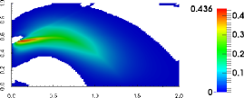
(a) $p=1$, XSeed = YSeed = 101

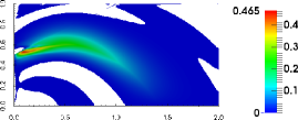
(b) $p=1$, XSeed = YSeed = 501

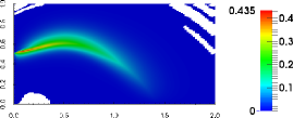
(c) $p=2$, XSeed = YSeed = 101

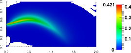
(d) $p=3$, XSeed = YSeed = 66

Figure 19. Plume development from boundary in a reaction tank (Type #2): This figure shows the concentration profiles of the product $C$ based on unconstrained primitive LSFEM. The white region indicates the area in which the obtained concentration is negative. The negative values are in the range $\mathcal{O}(10^{-3})$ to $\mathcal{O}(10^{-5})$. Both $h$-refinement and $p$-refinement could not eliminate the violation in the non-negative constraint for this problem, which has highly heterogeneous anisotropic diffusivity.

1. The violation of the non-negative constraint is small only for pure diffusion equations with isotropic diffusivity. The violations can be large in the case of anisotropic diffusion. If the maximum eigenvalue is not much smaller than unity, then naive $h/p$-refinement will not always reduce the negative values and clipping procedure can give erroneous results. Figure 19 and problem 6.2 in the paper illustrate this point. This has been illustrated even for diffusion equations in Reference [35].

2. Although tensorial dispersion frequently arises in the modeling of subsurface systems, many practitioners employ isotropic diffusion in their numerical simulations just to avoid large non-negative violations in their reactive-transport modeling. As mentioned earlier, in the case of isotropic diffusion, one can go away with the clipping procedure. But there is a need for predictive simulations for realistic scenarios (e.g., anisotropic diffusivity), and one needs carefully designed computational frameworks. Simple approaches like the clipping procedure will not suffice.

3. A clipping procedure, by itself, does not ensure local species balance.

4. The clipping procedure cannot eliminate the spurious node-to-node oscillations.

5. The ramifications of clipping the negative values on the species balance and on the overall accuracy of solutions have not been carefully studies or documented.

6. Finally, both $h$- and $p$-refinements may decrease the negative values and reduce spurious node-to-node oscillations for advection-dominated and reaction-dominated ADR problems. However, our objective is to satisfy maximum principles, non-negative constraint, species balance, reduce spurious node-to-node oscillations, and obtain sufficiently accurate numerical solutions on coarse computational grids. Extensive mesh and polynomial refinements defeats the main purpose, as these approaches will incur excessive computational cost.

3.2. Approach #2: Mesh restrictions

Recently, there has been a surge on the study of constructing meshes to satisfy various discrete maximum principles both within the context of single-field and mixed finite element formulations [36, 37, 38]. The primary objective of these methods is to develop restrictions on the computational meshes to meet the underlying principles. However, it should be noted that there are various drawbacks for these methods. The important ones are described as follows:

1. Most of these mesh restriction methods are for simplicial meshes (such as three-node triangular element and four-node tetrahedral element). Extending these results to non-simplicial elements is not trivial or may not be possible.

2. The boundary conditions are restricted to only Dirichlet on the entire boundary of the domain. Incorporating mixed boundary conditions or a general Neumann BC given by equation (2.1c) has not been addressed.

3. Generating a DMP-based mesh for complex domains is extremely difficult and sometimes impossible.

4. For highly advection-dominated and reaction-dominated problems, we need a highly refined DMP-based meshes. Constructing such meshes is computationally intensive.

5. Even though the mesh restriction conditions put forth for the weak Galerkin method by Huang and Wang [37] is locally conservative, it is restricted to pure anisotropic diffusion equations. Generalizing it to obtain locally conservative DMP-based meshes for anisotropic ADR equations is not apparent. Moreover, it still suffers from the above set of drawbacks.

3.3. Approach #3: Using non-negative methodologies for diffusion equations

Recently, optimization-based finite element methods [15, 16, 17, 35] are proposed to satisfy the non-negative constraint and maximum principles for diffusion-type equations. These non-negative methodologies are for self-adjoint operators and are constructed by invoking Vainberg’s theorem [39]. That is, they utilize the fact that there exists a scalar functional such that the Gâteaux variation of this functional provides the weak formulation and the Euler-Lagrange equations provide the corresponding governing equations for the diffusion problem. Corresponding to this continuous variational/minimization functional, a discrete non-negative constrained optimization-based finite element method is developed. Unfortunately, such a variational principle based on Vainberg’s theorem does not exist for the Galerkin weak formulation for an ADR equation, as the spatial operator is non-self-adjoint [40].

3.4. Approach #4: Posing the discrete equations as a $P$-LCP

Let $h$ be the maximum element size, $\|\mathbf{v}\|_{\infty,\Omega}$ be the maximum value for advection velocity field, $\alpha_{\infty,\Omega}$ be the maximum value for linear reaction coefficient, and $\lambda_{\mathrm{min}}$ be the minimum eigenvalue of $\mathbf{D}(\mathbf{x})$ in the entire domain. Mathematically, these quantities are defined as follows:

$$h :=\displaystyle\mathop{\mbox{max}}_{\Omega_{e}\in\Omega_{h}}\left[h_{\Omega_{e}}\right]$$ (3.1a)

$$\|\mathbf{v}\|_{\infty,\Omega} :=\displaystyle\mathop{\mbox{max}}_{1\leq i\leq nd}\left[|(\mathbf{v}(\mathbf{x}))_{i}|\right]\quad\forall\mathbf{x}\in\Omega$$ (3.1b)

$$\alpha_{\infty,\Omega} :=\displaystyle\mathop{\mbox{max}}_{\mathbf{x}\in\Omega}\left[\alpha(\mathbf{x})\right]$$ (3.1c)

$$\lambda_{\mathrm{min}} :=\displaystyle\mathop{\mbox{min}}_{\mathbf{x}\in\Omega}\left[\lambda_{\mathrm{min},\mathbf{D}(\mathbf{x})}\right]$$ (3.1d)

$$\lambda_{\mathrm{max}} :=\displaystyle\mathop{\mbox{max}}_{\mathbf{x}\in\Omega}\left[\lambda_{\mathrm{max},\mathbf{D}(\mathbf{x})}\right]$$ (3.1e)

where $\Omega_{h}$ is a regular linear finite element partition of the domain $\Omega$ such that $\overline{\Omega}_{h}=\bigcup_{e=1}^{Nele}\overline{\Omega}_{\mathrm{e}}$. “Nele” is the total number of discrete non-overlapping open sub-domains. The boundary of $\Omega_{\mathrm{e}}$ is denoted as $\partial\Omega_{\mathrm{e}}:=\overline{\Omega}_{\mathrm{e}}-\Omega_{\mathrm{e}}$. $h_{\Omega_{e}}$ is the diameter of element $\Omega_{e}$. $\lambda_{\mathrm{min},\mathbf{D}(\mathbf{x})}$ and $\lambda_{\mathrm{max},\mathbf{D}(\mathbf{x})}$ are, respectively, the minimum and maximum eigenvalue of $\mathbf{D}(\mathbf{x})$ at a given point $\mathbf{x}\in\Omega$. Correspondingly, the element Péclet number $\mathbb{P}\mathrm{e}_{h}$ and the element Damköhler number $\mathbb{D}\mathrm{a}_{h}$ are defined as follows:

$$\mathbb{P}\mathrm{e}_{h} :=\frac{\|\mathbf{v}\|_{\infty,\Omega}h}{2\lambda_{\mathrm{min}}}$$ (3.2a)

$$\mathbb{D}\mathrm{a}_{h} :=\frac{\alpha_{\infty,\Omega}h^{2}}{\lambda_{\mathrm{min}}}$$ (3.2b)

Herein, $\mathbb{D}\mathrm{a}_{h}$ is defined based on linear reaction coefficient and diffusivity. However, it should be noted that there are various ways to construct different types of element Damköhler numbers (for instance, see Reference [41] for isotropic diffusivity).

After low-order finite element discretization of either $\mathrm{SG}_{1}$ or $\mathrm{SG}_{2}$, the discrete equations for the ADR boundary value problem take the following form:

$$\boldsymbol{K}\boldsymbol{c}=\boldsymbol{f}$$ (3.3)

where $\boldsymbol{K}$ is the stiffness matrix (which is neither symmetric nor positive definite), $\boldsymbol{c}$ is the vector containing nodal concentrations, and $\boldsymbol{f}$ is the volumetric source vector. The matrix $\boldsymbol{K}$ is of size $ncdofs\times ncdofs$, where “$ncdofs$” denotes the number of free degrees-of-freedom for the concentration. The vectors $\boldsymbol{c}$ and $\boldsymbol{f}$ are of size $ncdofs\times 1$.

In the rest of this paper, the symbols $\succeq$ and $\preceq$ will be used to denote the component-wise comparison of vectors and matrices. That is, given two vectors $\boldsymbol{a}$ and $\boldsymbol{b}$, $\boldsymbol{a}\preceq\boldsymbol{b}$ means that $(\boldsymbol{a})_{i}\leq(\boldsymbol{b})_{i}$ for all $i$. Likewise, given two matrices $\boldsymbol{A}$ and $\boldsymbol{B}$, $\boldsymbol{A}\preceq\boldsymbol{B}$ means that $(\boldsymbol{A})_{ij}\leq(\boldsymbol{B})_{ij}$ for all $i$ and $j$. The mathematical means of the symbols $\succeq$, $\prec$ and $\succ$ should now be obvious. We shall use $\boldsymbol{0}$ and $\boldsymbol{O}$ to denote zero vector and zero matrix, respectively.

Definition 3.1 ($P$-matrix, $Z$-matrix, and $M$-matrix).

A matrix $\boldsymbol{A}\in\mathbb{R}^{nd\times nd}$ is a $P$-matrix if $\frac{1}{2}\left(\boldsymbol{A}+\boldsymbol{A}^{\mathrm{T}}\right)$ is positive-definite. The matrix is a $Z$-matrix if $(\boldsymbol{A})_{ij}\leq 0$, where $i\neq j$ and $i,j=1,\cdots,nd$. The matrix is an $M$-matrix if $\boldsymbol{A}$ is a $P$-matrix and a $Z$-matrix.

Definition 3.2 (Coarse mesh demarcation for anisotropic ADR equations).

A regular low-order finite element computational mesh $\Omega_{h}$ is said to be coarse with respect to

1. spurious oscillations if $\mathbb{P}\mathrm{e}_{h}>1$

2. spurious oscillations and large linear reaction coefficient if $\mathbb{P}\mathrm{e}_{h}>1$ and $\mathbb{D}\mathrm{a}_{h}>1$

3. spurious oscillations, large linear reaction coefficient, and a discrete maximum principle if the stiffness matrix $\boldsymbol{K}$ associated with either $\mathrm{SG}_{1}$ or $\mathrm{SG}_{2}$ is not an $M$-matrix

It can be easily shown through counterexamples that the stiffness matrix $\boldsymbol{K}$ for ADR equation will not always be a $Z$-matrix. We shall now provide two such counterexamples. The first counterexample is the low-order finite element discretization based on two-node linear element for the following 1D ADR equation (with constant velocity, diffusivity, and linear reaction coefficients):

$$\alpha c+v\frac{dc}{dx}-D\frac{d^{2}c}{dx^{2}}=f(x)\quad\forall x\in\Omega:=(0,1)$$ (3.4a)

$$c(x)=c^{\mathrm{p}}(x)\quad\forall x\in\partial\Omega:=\{0,1\}$$ (3.4b)

with $\alpha\geq 0$, $D>0$, and $v\in\mathbb{R}$. The entries of stiffness matrix $\boldsymbol{K}$ for an $i^{\mathrm{th}}$ intermediate node (using equal-sized two-node linear finite element) is given as follows:

$$\frac{\alpha h}{6}\left[\begin{array}[]{ccc}1&4&1\end{array}\right]\left\{\begin{array}[]{c}c_{i-1}\\ c_{i}\\ c_{i+1}\end{array}\right\}+\frac{v}{2}\left[\begin{array}[]{ccc}-1&0&1\end{array}\right]\left\{\begin{array}[]{c}c_{i-1}\\ c_{i}\\ c_{i+1}\end{array}\right\}+\frac{D}{h}\left[\begin{array}[]{ccc}-1&2&-1\end{array}\right]\left\{\begin{array}[]{c}c_{i-1}\\ c_{i}\\ c_{i+1}\end{array}\right\}$$ (3.17)

On trivial manipulations on equation (3.17), it is evident that the stiffness matrix is a $Z$-matrix if and only if the following condition is satisfied:

$$h\leq h_{\mathrm{max}}:=\frac{12D}{3|v|+\sqrt{9v^{2}+24\alpha D}}$$ (3.18)

which is not always the case. The second counterexample is based on a simplicial finite element discretization (e.g., three-node triangular/four-node tetrahedron element) of ADR equation with Dirichlet BCs on the entire boundary. If any $nd$-simplicial mesh does not satisfy the following condition then $\boldsymbol{K}$ is not a $Z$-matrix [38, Theorem 4.3]:

$$0<\frac{h_{p}\,\|\mathbf{v}\|_{\infty,\overline{\Omega}_{e}}}{(nd+1)\,\Lambda_{\mathrm{min},\widetilde{\boldsymbol{D}}_{\Omega_{e}}}} +\frac{h_{p}\,h_{q}\,\alpha_{\infty,\overline{\Omega}_{e}}}{(nd+1)\,(nd+2)\,\Lambda_{\mathrm{min},\widetilde{\boldsymbol{D}}_{\Omega_{e}}}}\leq\cos(\beta_{pq,\widetilde{\boldsymbol{D}}^{-1}_{\Omega_{e}}})$$

$$\forall p,q=1,2,\cdots,nd+1,\;p\neq q,\;\Omega_{e}\in\Omega_{h}$$ (3.19)

where $p$ and $q$ are the any two given arbitrary vertices of $\Omega_{e}$. $\widetilde{\boldsymbol{D}}_{\Omega_{e}}$ is the integral element average anisotropic diffusivity. $\Lambda_{\mathrm{min},\widetilde{\boldsymbol{D}}_{\Omega_{e}}}$ denotes the minimum eigenvalue of $\widetilde{\boldsymbol{D}}_{\Omega_{e}}$. $h_{p}$ and $h_{q}$ are the perpendicular distance (or the height) from vertices $p$ and $q$ to their respective opposite faces. $\beta_{pq,\widetilde{\boldsymbol{D}}^{-1}_{\Omega_{e}}}$ is the dihedral angle measured in $\widetilde{\boldsymbol{D}}^{-1}_{\Omega_{e}}$ metric between two faces opposite to vertices $p$ and $q$ of an element $\Omega_{e}$.

Proposition 3.3 ($P$-matrix linear complementarity problem for ADR equations).

Given that assumptions (A1)–(A5) hold, then the stiffness matrix $\boldsymbol{K}$ associated with low-order finite element discretization of either $\mathrm{SG}_{1}$ or $\mathrm{SG}_{2}$ is a $P$-matrix. Furthermore, if $\boldsymbol{c}$ has to be DMP-preserving on any arbitrary coarse mesh, then the resulting constrained discrete equations of single-field Galerkin formulation can be posed as a $P$-$\mathrm{LCP}$.

Proof.

We prove only for $\mathrm{SG}_{1}$ formulation and extending it to $\mathrm{SG}_{2}$ is a trivial manipulation. The symmetric part of the element stiffness matrix $\boldsymbol{K}_{e}$ is given as follows:

$$\frac{1}{2}\left(\boldsymbol{K}_{e}+\boldsymbol{K}_{e}^{\mathrm{T}}\right)=\int\limits_{\Omega_{e}}\left(\alpha(\mathbf{x})+\frac{1}{2}\mathrm{div}[\mathbf{v}(\mathbf{x})]\right)\boldsymbol{N}^{\mathrm{T}}\boldsymbol{N}\;\mathrm{d}\Omega_{e}\, +\,\int\limits_{\Omega_{e}}\boldsymbol{B}\mathbf{D}(\mathbf{x})\boldsymbol{B}^{\mathrm{T}}\;\mathrm{d}\Omega_{e}$$

$$+\int\limits_{\Gamma^{q}_{e}}\frac{1}{2}|\mathbf{v}\bullet\widehat{\mathbf{n}}|\boldsymbol{N}^{\mathrm{T}}\boldsymbol{N}\;\mathrm{d}\Gamma^{q}_{e}$$ (3.20)

where $\boldsymbol{N}$ is row vector containing shape functions and $\boldsymbol{B}=(\boldsymbol{DN})\boldsymbol{J}^{-1}$ (see Appendix A for details on $\boldsymbol{DN}$ and $\boldsymbol{J}$). From equation (3.4) and assumptions (A1)–(A5), it is evident $\frac{1}{2}\left(\boldsymbol{K}_{e}+\boldsymbol{K}_{e}^{\mathrm{T}}\right)$ is positive semi-definite. Furthermore, the assembly procedure ensures that the global stiffness matrix $\boldsymbol{K}$ is positive definite [42, Section 2 and Section 3]. As the mesh is coarse, $\boldsymbol{K}$ is not an $M$-matrix. But we want $\boldsymbol{c}$ to satisfy the DMP constraints. Hence, this results in the following constrained discrete system of equations:

$$\boldsymbol{K}\boldsymbol{c} =\boldsymbol{f}+\boldsymbol{\lambda}$$ (3.21a)

$$\boldsymbol{\lambda} \succeq\boldsymbol{0}$$ (3.21b)

$$\boldsymbol{c} \succeq\boldsymbol{0}$$ (3.21c)

$$\boldsymbol{\lambda}\bullet\boldsymbol{c} =0$$ (3.21d)

As $\boldsymbol{K}$ is a $P$-matrix, the above system is a $P$-matrix linear complementarity problem. This completes the proof. ∎

It needs to be emphasized that solving a LCP problem with P-matrix is, in general, NP-hard [43]. Therefore, posing the discrete equations as a LCP problem and numerically solving it is not a viable approach, especially for large-scale ADR problems with high $\mathbb{P}\mathrm{e}_{h}$. Moreover, it is not always feasible to find a DMP-based $h$-refined mesh that will produce accurate results for ADR equation for sufficiently high element Péclet number and element Damköhler number.

3.5. Approach #5: Posing the discrete problem as constrained normal equations

One way of constructing an optimization-based approach to meet the non-negative constraint is to rewrite the discrete problem as the following constrained normal equations:

$$\mathop{\mathrm{minimize}}_{\boldsymbol{c}\,\in\,\mathbb{R}^{ncdofs}} \quad\frac{1}{2}\langle\boldsymbol{c};\boldsymbol{K}^{\mathrm{T}}\boldsymbol{K}\boldsymbol{c}\rangle-\langle\boldsymbol{c};\boldsymbol{K}^{\mathrm{T}}\boldsymbol{f}\rangle$$ (3.22a)

subject to $$\quad\boldsymbol{c}\succeq\boldsymbol{0}$$ (3.22b)

where $\langle\bullet;\bullet\rangle$ denotes the standard inner-product in Euclidean spaces. The corresponding first-order optimality conditions can be written as:

$$\boldsymbol{K}^{\mathrm{T}}\boldsymbol{K}\boldsymbol{c}=\boldsymbol{K}^{\mathrm{T}}\boldsymbol{f}+\boldsymbol{\lambda}$$ (3.23a)

$$\boldsymbol{c}\succeq\boldsymbol{0}$$ (3.23b)

$$\boldsymbol{\lambda}\succeq\boldsymbol{0}$$ (3.23c)

$$\lambda_{i}c_{i}=0\quad\forall i=1,\cdots,ncdofs$$ (3.23d)

If there are no constraints, the optimization problem becomes:

$$\mathop{\mathrm{minimize}}_{\boldsymbol{c}\,\in\,\mathbb{R}^{ncdofs}} \quad\frac{1}{2}\langle\boldsymbol{c};\boldsymbol{K}^{\mathrm{T}}\boldsymbol{K}\boldsymbol{c}\rangle-\langle\boldsymbol{c};\boldsymbol{K}^{\mathrm{T}}\boldsymbol{f}\rangle$$ (3.24)

The first-order optimality condition for the unconstrained discrete optimization problem is:

$$\boldsymbol{K}^{\mathrm{T}}\boldsymbol{K}\boldsymbol{c}=\boldsymbol{K}^{\mathrm{T}}\boldsymbol{f}$$ (3.25)

In the numerical mathematics literature (e.g., see [44]), the above system of equations (3.25) is referred to as normal equations. The three main deficiencies of this approach are:

1. The constrained optimization-based normal equations method does not avoid node-to-node spurious oscillations. In addition, there is no obvious way of fixing the method to avoid this type of unphysical solutions.

2. It is well-known that the condition number of $\boldsymbol{K}^{\mathrm{T}}\boldsymbol{K}$ will be much worse than $\boldsymbol{K}$. So the numerical solution will be less reliable, less accurate, and numerically not stable [44].

3. The discrete optimization problem given by equation (3.24) on which non-negative constraints are enforced does not have a corresponding continuous variational/minimization problem.

We shall use the following academic problem to illustrate the aforementioned deficiencies:

$$v\frac{dc}{dx}-D\frac{d^{2}c}{dx^{2}}=f\quad\forall x\in(0,1)$$ (3.26a)

$$c(x=0)=c(x=1)=0$$ (3.26b)

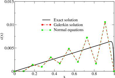
Figure 2. Academic problem: This figure compares the numerical solutions under the standard single-field Galerkin formulation and the normal equations approach with the exact solution. The normal equations approach does not eliminate node-to-node spurious oscillations.

where $v$, $D$, and $f$ are assumed to be constants. In our numerical experiment, we have taken the number of mesh elements to be 11, $v/D=150$, and $f=1$. The element Péclet number ($\mathbb{P}\mathrm{e}_{h}=\frac{vh}{2D}$) is approximately 6.82. Since it is greater than unity, there be will spurious node-to-node oscillations under the standard single-field Galerkin formulation. From Figure 2, it is evident that the normal equations approach does not eliminate the spurious node-to-node oscillations. The condition number of the stiffness matrix under the standard single-field Galerkin formulation is 8.41, whereas the condition number of the stiffness matrix under the normal equations approach is 70.69. For small element Péclet numbers, deficiency (i) can be avoided. But deficiencies (ii) and (iii) will still be present and cannot be circumvented. Hence, posing the discrete problem as constrained normal equations is not a viable approach to meet maximum principles and the non-negative constraint.

4. PROPOSED COMPUTATIONAL FRAMEWORK

We employ least-squares formalism to develop a class of structure-preserving numerical formulations whose solutions satisfy DMP, LSB, and GSB. The formulations are built based on minimization of unconstrained/constrained quadratic least-squares functionals. In a least-squares-based finite element formulation, a non-physical least-squares functional is constructed in terms of the sum of the squares of the residuals in an appropriate norm. These residuals are based on the underlying governing equations. However, it should be noted that LSFEMs are different from the Galerkin least-squares or stabilized mixed methods, where least-squares terms are added locally or globally to variational problems.

The success of LSFEM is due to the rich mathematical foundations that influence both the analysis and the algorithmic development. LSFEM offers several attractive features. The resulting weak formulations are coercive. Hence, a unique global minimizer exists for the least-squares functional and this minimizer coincides with the exact solution. Conforming finite element discretizations of least-squares functionals leads to stable and (eventually) optimally accurate numerical solutions. For mixed LSFEM-based formulations, equal order interpolation can be used for all the unknowns, which is computationally the most convenient. The resulting algebraic system is symmetric and positive definite. Thus, the discrete system can be solved using standard and robust iterative numerical methods. For more details on LSFEM for various applications, see Bochev and Gunzberger [45] and Jiang [46].

4.1. Design synopsis of the proposed numerical methodology

The central idea of the proposed computational framework is to constrain a least-squares functional with LSB and non-negative constraints. The main steps involved in the design of the proposed computational framework are:

1. The governing equations of the ADR problem are written in first-order mixed form.

2. We construct a stabilized least-squares functional for these first-order governing equations.

3. We construct algebraic equality constraints to enforce element-wise/local species balance (LSB).

4. We enforce bound constraints to the constructed LSFEM to meet maximum principles and the non-negative constraint in the discrete setting. In order to achieve this, we shall use low-order finite element interpolation for $c(\mathbf{x})$.

The first-order mixed form of the governing equations can be written as:

$$\mathbf{q}(\mathbf{x})-\mathbf{v}(\mathbf{x})c(\mathbf{x})+\mathbf{D}(\mathbf{x})\mathrm{grad}[c(\mathbf{x})]=\mathbf{0}\quad \mathrm{in}\;\Omega$$ (4.1a)

$$\mathrm{div}[\mathbf{q}(\mathbf{x})]=f(\mathbf{x})-\alpha(\mathbf{x})c(\mathbf{x})\quad \mathrm{in}\;\Omega$$ (4.1b)

$$c(\mathbf{x})=c^{\mathrm{p}}(\mathbf{x})\quad \mathrm{on}\;\Gamma^{c}$$ (4.1c)

$$\left(\mathbf{q}(\mathbf{x})-\left(\frac{1+\mathrm{Sign}[\mathbf{v}\bullet\widehat{\mathbf{n}}]}{2}\right)\mathbf{v}(\mathbf{x})c(\mathbf{x})\right)\bullet\widehat{\mathbf{n}}(\mathbf{x})=q^{\mathrm{p}}(\mathbf{x})\quad \mathrm{on}\;\Gamma^{q}$$ (4.1d)

The bound constraints to meet discrete maximum principles take the following form:

$$c_{\mathrm{min}}\boldsymbol{1}\preceq\boldsymbol{c}\preceq c_{\mathrm{max}}\boldsymbol{1}\quad\mathrm{in}\;\overline{\Omega}_{h}$$ (4.2)

where $c_{\mathrm{min}}$ and $c_{\mathrm{max}}$ are the minimum and maximum concentration values possible in $\overline{\Omega}$. The LSB equality constraints can be constructed in two different ways. The first approach is based on the integral statement of the balance of species on an element, and takes the following mathematical form:

$$\int\limits_{\Omega_{e}}\alpha(\mathbf{x})c(\mathbf{x})\;\mathrm{d}\Omega_{e}+\int\limits_{\partial\Omega_{e}}\mathbf{q}(\mathbf{x})\bullet\widehat{\mathbf{n}}(\mathbf{x})\;\mathrm{d}\Gamma_{e}=\int\limits_{\Omega_{e}}f(\mathbf{x})\;\mathrm{d}\Omega_{e}$$ (4.3)

The second approach is to enforce equation (4.1b) in each mesh element $\overline{\Omega}_{\mathrm{e}}$ in an integral form:

$$\int\limits_{\Omega_{e}}\alpha(\mathbf{x})c(\mathbf{x})\;\mathrm{d}\Omega_{e}+\int\limits_{\Omega_{e}}\mathrm{div}[\mathbf{q}(\mathbf{x})]\;\mathrm{d}\Omega_{e}=\int\limits_{\Omega_{e}}f(\mathbf{x})\;\mathrm{d}\Omega_{e}$$ (4.4)

One can obtain equation (4.3) by applying the divergence theorem to equation (4.4), which means that these two approaches are equivalent in the continuous setting. This will not always be the case in the discrete setting. In the case of simplicial and non-simplicial low-order finite elements, these approaches are equivalent. However, these two approaches can be different in the case of higher-order finite elements. This is because in certain higher-order finite elements (e.g., nine-node quadrilateral element), not all the nodes are on the boundary of the element. The flux at an interior node contributes to the second integral in equation (4.4) but not to the corresponding term in equation (4.3). These issues are beyond the scope of this paper. Herein, we take the first approach given by equation (4.3).

We next construct two different least-squares functionals and analyze the influence of various constraints on the performance of these LSFEMs. It should be noted that Hsieh and Yang [14] have proposed similar least-squares functionals, but they considered homogeneous isotropic steady-state advection-diffusion equations. Moreover, even in the simple setting of isotropic diffusivity, they did not consider general Neumann BCs, spatially varying velocity fields, simplicial vs. non-simplicial elements, or the effects of DMPs and LSB on the performance of the least-squares functionals. This paper investigates all the mentioned aspects: we incorporate anisotropy, heterogeneity, transient effects, linear reaction terms, non-solenoidal spatially varying velocity fields, and DMP and LSB constraints.

4.2. Weighted primitive LSFEM

The weighted primitive LSFEM is the standard way of constructing a LSFEM-based formulation. It does not contain any additional stabilization terms. The weighted primitive least-squares functional $\mathfrak{F}_{\mathrm{Prim}}(c,\mathbf{q}):\mathcal{C}\times\mathcal{Q}\rightarrow\mathbb{R}$ in $L_{2}$-norm can be written as:

$$\mathfrak{F}_{\mathrm{Prim}}\left(c,\mathbf{q}\right) :=\frac{1}{2}\Big{\|}\mathbf{A}(\mathbf{x})\big{(}\mathbf{q}-c\mathbf{v}+\mathbf{D}\mathrm{grad}[c]\big{)}\Big{\|}^{2}_{\Omega}$$

$$+\frac{1}{2}\Big{\|}\beta(\mathbf{x})\big{(}\alpha c+\mathrm{div}[\mathbf{q}]-f\big{)}\Big{\|}^{2}_{\Omega}$$

$$+\frac{1}{2}\Bigg{\|}\left(\mathbf{q}-\left(\frac{1+\mathrm{Sign}[\mathbf{v}\bullet\widehat{\mathbf{n}}]}{2}\right)c\mathbf{v}\right)\bullet\widehat{\mathbf{n}}-q^{\mathrm{p}}\Bigg{\|}^{2}_{\Gamma^{q}}$$ (4.5)

where the second-order tensor $\mathbf{A}(\mathbf{x})$ and the scalar function $\beta(\mathbf{x})$ are the weights, which are defined as follows:

$$\mathbf{A}(\mathbf{x}) =\left\{\begin{array}[]{cl}\mathbf{I}&\text{LS Type-1 }\\ \mathbf{D}^{-1/2}(\mathbf{x})&\text{LS Type-2}\end{array}\right.$$ (4.6c)

$$\beta(\mathbf{x}) =\left\{\begin{array}[]{cl}1&\text{LS Type-1}\\ \left.\begin{aligned} 1\qquad&\quad\text{if }\alpha(\mathbf{x})=0\\ \alpha^{-1/2}(\mathbf{x})&\quad\text{if }\alpha(\mathbf{x})\neq 0\end{aligned}\right\}&\text{LS Type-2}\end{array}\right.$$ (4.6f)

A corresponding weak form can be obtained by setting the Gâteaux variation of the functional (4.2) to zero. We shall show in Sections 5 and 6 that a naive way of constructing LSFEM formulation, just like the weighted primitive LSFEM, does not perform well for advection-dominated ADR problems. Moreover, enforcing LSB and DMP constraints do not seem to have a profound effect. In order to adequately capture steep boundary and interior layers, we introduce an alternate stabilized LSFEM formulation, which will be referred to as the weighted negatively stabilized streamline diffusion LSFEM. This stabilized LSFEM formulation will be able to handle a wide spectrum of ADR problems ranging from advection-dominated to reaction-dominated problems.

4.3. Weighted negatively stabilized streamline diffusion LSFEM

The underlying idea of the proposed stabilized LSFEM formulation is to combine the streamline diffusion and stabilized Galerkin formulations. This is motivated by the prior studies that combining these two formulations exhibit enhanced stability (for example, see [47, 14]). In this formulation, we introduce a small element-wise stabilization parameter $\delta_{\Omega_{\mathrm{e}}}$ to correct $\mathbf{q}(\mathbf{x})$ in the streamline direction by adding second-order derivatives of $c(\mathbf{x})$. The modified flux along the streamline direction takes the following form:

$$\mathbf{q}=c\mathbf{v}-\mathbf{D}\mathrm{grad}[c]+\delta_{\Omega_{\mathrm{e}}}\mathbf{v}\left(\mathrm{div}[c\mathbf{v}-\mathbf{D}\mathrm{grad}[c]]\right)$$ (4.7)

The basic philosophy of the correction to the flux given by equation (4.7) is in the spirit of stabilized finite element formulations such as SUPG [48, 47]. This flux correction is different from that of the Flux-Corrected Transport (FCT) methods [49]. Correspondingly, the species balance equation accounting for these corrections will be:

$$\alpha c+\mathrm{div}[\mathbf{q}]=f+f_{\delta_{\Omega_{\mathrm{e}}}}$$ (4.8)

where

$$f_{\delta_{\Omega_{\mathrm{e}}}}:=\delta_{\Omega_{\mathrm{e}}}\big{(}\mathrm{grad}[f-\alpha c]\bullet\mathbf{v}+\mathrm{div}[\mathbf{v}]\,\left(f-\alpha c\right)\big{)}$$ (4.9)

The modification to the flux (given by equations (4.7)–(4.9)) will present two different ways of constructing Neumann BCs.

The first way utilizes the quantities $\mathbf{q}(\mathbf{x})$, $c(\mathbf{x})$, $\alpha(\mathbf{x})$, and $f(\mathbf{x})$, and takes the following form:

$$\left(\mathbf{q}-\left(\frac{1+\mathrm{Sign}[\mathbf{v}\bullet\widehat{\mathbf{n}}]}{2}\right)c\mathbf{v}-\delta_{\Omega_{\mathrm{e}}}\left(f-\alpha c\right)\mathbf{v}\right)\bullet\widehat{\mathbf{n}}(\mathbf{x})=q^{\mathrm{p}}(\mathbf{x})\quad\mathrm{on}\;\Gamma^{q}$$ (4.10)

The second way utilizes $\mathbf{q}(\mathbf{x})$, $c(\mathbf{x})$, and the first and second derivatives of $c(\mathbf{x})$. The corresponding expression for Neumann BCs takes the following form:

$$\left(\mathbf{q}-\left(\frac{1+\mathrm{Sign}[\mathbf{v}\bullet\widehat{\mathbf{n}}]}{2}\right)c\mathbf{v}-\delta_{\Omega_{\mathrm{e}}}\left(\mathrm{div}[c\mathbf{v}-\mathbf{D}\mathrm{grad}[c]]\right)\mathbf{v}\right)\bullet\widehat{\mathbf{n}}(\mathbf{x})=q^{\mathrm{p}}(\mathbf{x})\quad\mathrm{on}\;\Gamma^{q}$$ (4.11)

In the continuous setting, equations (4.10) and (4.11) are equivalent. However, in the discrete setting, the performance of these equations can be different based on the kind of (finite) element being employed. For example, for simplicial elements (such as three-node triangular (T3) element and four-node tetrahedral (T4) element) and four-node quadrilateral (Q4) element, both $\mathrm{div}[\mathrm{grad}[c(\mathbf{x})]]$ and $\mathrm{grad}[\mathrm{grad}[c(\mathbf{x})]]$ are zero for $\overline{\Omega}_{\mathrm{e}}\in{\Gamma^{q}}$. This is because the Hessian of $\boldsymbol{N}$, which is $\boldsymbol{DDN}$, is a zero matrix for both two-node linear (L2) and three-node triangular elements. For more details, see Appendix A. But, this is not the case with non-simplicial linear finite elements for $nd=3$ and higher-order finite elements (in any dimension). Hence, the Neumann BCs based on equation (4.11) are not always physically consistent. However, Neumann BCs based on equation (4.10) are always consistent irrespective of the finite element used. Herein, we have chosen Neumann BCs given by equation (4.10).

Based on the above set of equations (4.7)–(4.10), we construct a $L_{2}$-norm based least-squares functional. Additionally, as in the Galerkin least-squares method, we add a stabilization term to this functional. This stabilization term is as follows:

$$\frac{1}{2}\sum_{\Omega_{\mathrm{e}}\in\Omega_{h}}\tau_{\Omega_{\mathrm{e}}}\Big{\|}\mathrm{div}\big{[}c\mathbf{v}-\mathbf{D}\mathrm{grad}[c]\big{]}+\alpha c-f\Big{\|}^{2}_{\Omega_{\mathrm{e}}}$$ (4.12)

The least-squares functional for the weighted negatively stabilized streamline diffusion formulation $\mathfrak{F}_{\mathrm{NgStb}}(c,\mathbf{q}):\mathcal{C}\times\mathcal{Q}\rightarrow\mathbb{R}$ in $L_{2}$-norm takes the following form:

$$\mathfrak{F}_{\mathrm{NgStb}}\left(c,\mathbf{q}\right) :=\frac{1}{2}\sum_{\Omega_{\mathrm{e}}\in\Omega_{h}}\Big{\|}\mathbf{A}(\mathbf{x})\big{(}\mathbf{q}-c\mathbf{v}+\mathbf{D}\mathrm{grad}[c]-\delta_{\Omega_{\mathrm{e}}}\mathbf{v}\left(\mathrm{div}[c\mathbf{v}-\mathbf{D}\mathrm{grad}[c]]\right)\big{)}\Big{\|}^{2}_{\Omega_{\mathrm{e}}}$$

$$+\frac{1}{2}\sum_{\Omega_{\mathrm{e}}\in\Omega_{h}}\Big{\|}\beta(\mathbf{x})\big{(}\alpha c+\mathrm{div}[\mathbf{q}]-f-f_{\delta_{\Omega_{\mathrm{e}}}}\big{)}\Big{\|}^{2}_{\Omega_{\mathrm{e}}}$$

$$+\frac{1}{2}\sum_{\Omega_{\mathrm{e}}\in{\Gamma^{q}}}\Bigg{\|}\left(\mathbf{q}-\left(\frac{1+\mathrm{Sign}[\mathbf{v}\bullet\widehat{\mathbf{n}}]}{2}\right)c\mathbf{v}-\delta_{\Omega_{\mathrm{e}}}\left(f-\alpha c\right)\mathbf{v}\right)\bullet\widehat{\mathbf{n}}-q^{\mathrm{p}}\Bigg{\|}^{2}_{\Omega_{\mathrm{e}}}$$

$$+\frac{1}{2}\sum_{\Omega_{\mathrm{e}}\in\Omega_{h}}\tau_{\Omega_{\mathrm{e}}}\Big{\|}\mathrm{div}\big{[}c\mathbf{v}-\mathbf{D}\mathrm{grad}[c]\big{]}+\alpha c-f\Big{\|}^{2}_{\Omega_{\mathrm{e}}}$$ (4.13)

The element dependent parameters $\tau_{\Omega_{\mathrm{e}}}\leq 0$ and $\delta_{\Omega_{\mathrm{e}}}\leq 0$ are given as:

$$\delta_{\Omega_{\mathrm{e}}} =-\frac{\delta_{o}\lambda_{\mathrm{min}}h^{2}_{\Omega_{\mathrm{e}}}}{\left(\lambda^{2}_{\mathrm{max}}+\delta_{1}\displaystyle\mathop{\mathrm{max}}_{\mathbf{x}\in\overline{\Omega}}\left[\left(\alpha+\mathrm{div}[\mathbf{v}]\right)^{2}\right]h^{2}+\delta_{2}\displaystyle\mathop{\mathrm{max}}_{\mathbf{x}\in\overline{\Omega}}\left[\|\mathrm{div}[\mathbf{D}]\|^{2}\right]h^{2}\right)}$$ (4.14a)

$$\tau_{\Omega_{\mathrm{e}}} =-\frac{\tau_{o}\lambda^{2}_{\mathrm{min}}h^{2}_{\Omega_{\mathrm{e}}}}{\left(\lambda^{2}_{\mathrm{max}}+\tau_{1}\displaystyle\mathop{\mathrm{max}}_{\mathbf{x}\in\overline{\Omega}}\left[\left(\alpha+\mathrm{div}[\mathbf{v}]\right)^{2}\right]h^{2}+\tau_{2}\displaystyle\mathop{\mathrm{max}}_{\mathbf{x}\in\overline{\Omega}}\left[\|\mathrm{div}[\mathbf{D}]\|^{2}\right]h^{2}\right)}$$ (4.14b)

where $\delta_{o}$, $\delta_{1}$, $\delta_{2}$, $\tau_{o}$, $\tau_{1}$, and $\tau_{2}$ are non-negative constants. Appendix B provides a thorough mathematical justification behind the above stabilization parameters.

For unconstrained LSFEMs, the errors incurred in satisfying LSB and GSB can be calculated as:

$$\epsilon^{(e)}_{\text{\tiny{LSB}}} =\int\limits_{\Omega_{e}}\alpha(\mathbf{x})c(\mathbf{x})\;\mathrm{d}\Omega+\int\limits_{\partial\Omega_{e}}\mathbf{q}(\mathbf{x})\bullet\widehat{\mathbf{n}}(\mathbf{x})\;\mathrm{d}\Gamma-\int\limits_{\Omega_{e}}f(\mathbf{x})\;\mathrm{d}\Omega$$ (4.15a)

$$\epsilon_{\text{\tiny{GSB}}} =\sum_{e=1}^{Nele}\epsilon^{(e)}_{\text{\tiny{LSB}}}$$ (4.15b)

where $c(\mathbf{x})$ and $\mathbf{q}(\mathbf{x})$ are the solutions obtained by solving a given unconstrained LSFEM. In numerical $h$-convergence study, we are interested in the following quantities with respect to $h$-refinement:

$$\epsilon_{\text{\tiny{MaxAbsLSB}}} =\mathop{\mathrm{max}}_{\Omega_{e}\in\Omega_{h}}\left[|\epsilon^{(e)}_{\text{\tiny{LSB}}}|\right]$$ (4.16)

$$\epsilon_{\text{\tiny{AbsGSB}}} =|\epsilon_{\text{\tiny{GSB}}}|$$ (4.17)

Few remarks about the species balance are in order. In writing equation (4.17), we have assumed that the mesh is conforming, and the test and trial functions belong to $C^{0}(\Omega)$ (i.e., there is inter-element continuity of the functions). Under the proposed computational framework, we place explicit (equality) constraints to meet $\epsilon^{(e)}_{\text{\tiny{LSB}}}=0\quad\forall e=1,\cdots,Nele$. By meeting the local species balance, the global species balance is trivially met.

4.4. Discrete equations

Let $\boldsymbol{K}_{cc}$ denote the stiffness matrix obtained by lower-order finite element discretization of the LSFEM terms involving $c(\mathbf{x})$ and $w(\mathbf{x})$. Similarly, we can define the stiffness matrices $\boldsymbol{K}_{c\mathbf{q}}$, $\boldsymbol{K}_{\mathbf{q}c}$, and $\boldsymbol{K}_{\mathbf{q}\mathbf{q}}$. The load vectors are denoted by $\boldsymbol{r}_{c}$ and $\boldsymbol{r}_{\mathbf{q}}$, respectively. These vectors are obtained from the finite element discretization of the LSFEM terms involving $w(\mathbf{x})$ and $\mathbf{p}(\mathbf{x})$. It should be noted that the stiffness matrices $\boldsymbol{K}_{cc}$ and $\boldsymbol{K}_{\mathbf{q}\mathbf{q}}$ are symmetric and positive definite. Furthermore, $\boldsymbol{K}_{\mathbf{q}c}=\boldsymbol{K}_{c\mathbf{q}}^{\mathrm{T}}$. For more details, see Appendix C.

The corresponding constrained optimization problem in the discrete setting for the proposed locally conservative DMP-preserving LSFEMs can be written as follows:

$$\mathop{\mathrm{minimize}}_{\begin{subarray}{c}\boldsymbol{c}\,\in\,\mathbb{R}^{ncdofs}\\ \boldsymbol{q}\,\in\,\mathbb{R}^{nqdofs}\end{subarray}} \quad\frac{1}{2}\langle\boldsymbol{c};\boldsymbol{K}_{cc}\boldsymbol{c}\rangle+\langle\boldsymbol{c};\boldsymbol{K}_{c\mathbf{q}}\boldsymbol{q}\rangle+\frac{1}{2}\langle\boldsymbol{q};\boldsymbol{K}_{\mathbf{q}\mathbf{q}}\boldsymbol{q}\rangle-\langle\boldsymbol{c};\boldsymbol{r}_{c}\rangle-\langle\boldsymbol{q};\boldsymbol{r}_{\mathbf{q}}\rangle$$ (4.18a)

subject to $$\quad\begin{cases}\boldsymbol{A}_{c}\boldsymbol{c}+\boldsymbol{A}_{\mathbf{q}}\boldsymbol{q}=\boldsymbol{b}_{f}\\ c_{\mathrm{min}}\boldsymbol{1}\preceq\boldsymbol{c}\preceq c_{\mathrm{max}}\boldsymbol{1}\end{cases}$$ (4.18b)

where “$nqdofs$” denotes the number of degrees-of-freedom for the flux vector, and “$ncdofs$” denotes the number of degrees-of-freedom for the concentration. The vector of size $ncdofs\times 1$ with all entries to be unity is denoted as $\mathbf{1}$. Recall that $\langle\bullet;\bullet\rangle$ denotes the standard inner-product on the Euclidean spaces. The finite element discretization of the local species balance equation gives rise to the global LSB matrices $\boldsymbol{A}_{c}$ and $\boldsymbol{A}_{\mathbf{q}}$, and the global LSB vector $\boldsymbol{b}_{f}$. The matrices $\boldsymbol{A}_{c}$ and $\boldsymbol{A}_{\mathbf{q}}$ are of sizes $Nele\times ncdofs$ and $Nele\times nqdofs$, respectively. Similar inference can be drawn on the sizes of $\boldsymbol{b}_{f}$, $\boldsymbol{r}_{c}$, $\boldsymbol{r}_{\mathbf{q}}$, $\boldsymbol{K}_{c\mathbf{q}}$, and $\boldsymbol{K}_{\mathbf{q}\mathbf{q}}$. Since $\boldsymbol{K}_{\mathbf{q}c}=\boldsymbol{K}_{c\mathbf{q}}^{\mathrm{T}}$ and the matrices $\boldsymbol{K}_{cc}$ and $\boldsymbol{K}_{\mathbf{q}\mathbf{q}}$ are symmetric and positive definite, the constrained optimization problem (4.18a)–(4.18b) belongs to convex quadratic programming and has a unique global minimizer [50]. The corresponding first-order optimality conditions – popularly known as the Karush-Kuhn-Tucker (KKT) conditions – for this discrete optimization problem take the following form:

$$\boldsymbol{K}_{cc}\boldsymbol{c}+\boldsymbol{K}_{c\mathbf{q}}\boldsymbol{q}=\boldsymbol{r}_{c}-\boldsymbol{A}^{\mathrm{T}}_{c}\boldsymbol{\lambda}_{c}+\boldsymbol{\mu}_{\mathrm{min}}-\boldsymbol{\mu}_{\mathrm{max}}$$ (4.19a)

$$\boldsymbol{K}_{c\mathbf{q}}^{\mathrm{T}}\boldsymbol{c}+\boldsymbol{K}_{\mathbf{q}\mathbf{q}}\boldsymbol{q}=\boldsymbol{r}_{\mathbf{q}}-\boldsymbol{A}^{\mathrm{T}}_{\mathbf{q}}\boldsymbol{\lambda}_{\mathbf{q}}$$ (4.19b)

$$\boldsymbol{A}_{c}\boldsymbol{c}+\boldsymbol{A}_{\mathbf{q}}\boldsymbol{q}=\boldsymbol{b}_{f}$$ (4.19c)

$$\boldsymbol{\mu}_{\mathrm{min}}\succeq\boldsymbol{0}$$ (4.19d)

$$\boldsymbol{\mu}_{\mathrm{max}}\succeq\boldsymbol{0}$$ (4.19e)

$$\left(\boldsymbol{c}-c_{\mathrm{min}}\boldsymbol{1}\right)\bullet\boldsymbol{\mu}_{\mathrm{min}}=0$$ (4.19f)

$$\left(c_{\mathrm{max}}\boldsymbol{1}-\boldsymbol{c}\right)\bullet\boldsymbol{\mu}_{\mathrm{max}}=0$$ (4.19g)

where $\boldsymbol{\lambda}_{c}$ and $\boldsymbol{\lambda}_{\mathbf{q}}$ are the Lagrange multipliers enforcing the LSB equality constraints, which stem from equation (4.19c). $\boldsymbol{\mu}_{\mathrm{min}}$ and $\boldsymbol{\mu}_{\mathrm{max}}$ are the KKT multipliers enforcing the DMP inequality constraints given by $c_{\mathrm{min}}\boldsymbol{1}\preceq\boldsymbol{c}$ and $\boldsymbol{c}\preceq c_{\mathrm{max}}\boldsymbol{1}$. Note that the non-negative constraint is a subset of the DMP inequality constraints. To wit, setting $c_{\mathrm{min}}=0$ and $c_{\mathrm{max}}=+\infty$ will result in explicit non-negative constraints on the nodal concentrations.

Remark 4.1.

Note that the continuous problem, in general, cannot always be written as an optimization problem. This is certainly the case with respect to ADR equation [40]. Moreover, in the continuous setting, the non-negative and local species balance constraints are satisfied trivially. Therefore, the Lagrange multipliers are zero in the continuous setting (if one can write the problem as an optimization problem). The violations of the non-negative and local species balance constraints are only in the discrete setting. This is the reason why one needs to obtain the discrete form before one can fix the deficiencies in solving the discrete equations.

In the next two sections, we illustrate the performance of the proposed computational framework for advection-dominated ADR problems and transport-controlled irreversible fast bimolecular reactions. In all the numerical simulations reported in this paper, the constrained optimization problem is solved using the MATLAB’s [33] built-in function handler quadprog, which has a robust solver based on an interior-point numerical algorithm presented in References [51, 52, 53]. One can alternatively employ the open-source optimization solvers such as COBYLA, SLSQP, L-BFGS-B, or TNC from SciPy [54]. The tolerance in the stopping criterion for solving convex quadratic programming problems is taken as $100\epsilon_{\mathrm{mach}}$, where $\epsilon_{\mathrm{mach}}\approx 2.22\times 10^{-16}$ is the machine precision for a 64-bit machine.

There are various approaches to numerically solve transient diffusion-type systems. It is desirable to have a numerical strategy that converts and utilizes the solvers for steady-state diffusion-type equations to solve transient systems. It has been recently shown that the method of horizontal lines using the backward Euler time-stepping scheme is one of the viable approaches to respect maximum principles and the non-negative constraint in the discrete setting [55]. The method of horizontal lines discretizes the time domain first, and thereby converts the transient ADR equations at each time-level into a system of governing equations similar to (2.1a)–(2.1c). This methodology, thus, helps us to use the computational framework provided in Section 4. One can employ a numerical procedure similar to Algorithm $1$ provided in Reference [55] to advance the numerical solution over the time. Numerical results for transient systems are presented in Section 6.

5. NUMERICAL $h$-CONVERGENCE AND BENCHMARK PROBLEMS

We shall employ a popular problem from the literature, which is commonly used to assess the accuracy of numerical formulations for advective-diffusive systems (e.g., see [56, 14]). The test problem is constructed using the method of manufactured solutions. The computational domain is a bi-unit square: $\Omega=(0,1)\times(0,1)$. The advection velocity vector field is taken as $\mathbf{v}(\mathbf{x})=\hat{\mathbf{e}}_{y}$, where $\hat{\mathbf{e}}_{y}$ is the unit vector along the $y$-direction. The scalar diffusivity is denoted by $D(\mathbf{x})$. The concentration field is taken as follows:

$$c(x,y)=\frac{\sin(\pi x)}{e^{m_{2}-m_{1}}-1}\left(e^{m_{2}-m_{1}}e^{m_{1}y}-e^{m_{2}y}\right)$$ (5.1)

where the constants $m_{1}$ and $m_{2}$ are given in terms of the scalar diffusivity:

$$m_{1}=\frac{1-\sqrt{1+4\pi^{2}D^{2}}}{2D}$$ (5.2a)

$$m_{2}=\frac{1+\sqrt{1+4\pi^{2}D^{2}}}{2D}$$ (5.2b)

We have taken $D(\mathbf{x})=10^{-2}$ in our numerical simulations. This choice is arbitrary, and is primarily motivated to check whether the proposed framework gives stable, reliable, and accurate numerical results for advection-dominated problems. For the chosen value of the diffusivity, the solution (5.1) exhibits steep gradients near the boundary of the domain. A pictorial description of the boundary value problem is provided by Figure 3.

Numerical solutions for the concentration and the flux vector are obtained by prescribing Dirichlet boundary conditions on all the four sides of the computational domain. These conditions are enforced strongly and are given as follows:

$$c(\mathbf{x})=\;\begin{cases}\sin(\pi x)\quad&\mathrm{for}\;y=0\\ 0\quad&\mathrm{for}\;x=0\;\mathrm{or}\;x=1\;\mathrm{or}\;y=1\end{cases}$$ (5.3)

Using equation (5.1), one can calculate the corresponding flux vector and volumetric source needed for the convergence analysis.

5.1. Convergence analysis for $D(x,y)=10^{-2}$

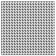
(a) Mesh using T3 elements

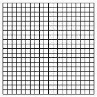
(b) Mesh using Q4 elements

Figure 4. Numerical $h$-convergence study: This figure shows the typical computational meshes used in the numerical convergence analysis. The meshes shown in this figure have 21 nodes along each side of the computational domain (i.e., XSeed = YSeed = 21). A series of hierarchical computational meshes are employed in the study with $11\times 11$, $21\times 21$, $41\times 41$ and $81\times 81$ nodes.

Herein, we will discuss the performance of negatively stabilized streamline diffusion LSFEM with and without LSB constraints. In case of unconstrained setting, we also quantify the errors incurred in satisfying LSB and GSB. Numerical simulations are performed using a series of hierarchical structured meshes based on three-node triangular (T3) and four-node quadrilateral (Q4) elements with XSeed and YSeed ranging from 11 to 81. Figure 4 provides the typical computational meshes used in the numerical $h$-convergence analysis.

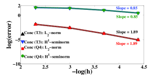
(a) Concentration: No constraints

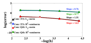
(b) Concentration: LSB constraints

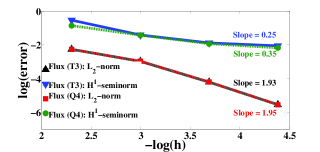
(c) Flux: No constraints

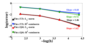
(d) Flux: LSB constraints

Figure 5. Numerical $h$-convergence study: This figure shows the convergence rates for the concentration and flux vector in $L_{2}$-norm and $H^{1}$-semi-norm with and without LSB constraints. Convergence studies are performed using T3- and Q4-based meshes under the negatively stabilized streamline diffusion LSFEM. It is evident that the Q4 element slightly outperforms the T3 element in terms of rates of convergence.

The weights for the primitive and negatively stabilized streamline diffusion LSFEMs are taken to be of LS Type-1 (i.e., $\mathbf{A}(\mathbf{x})=\mathbf{I}$ and $\beta(\mathbf{x})=1$). The element stabilization parameters for negatively stabilized streamline diffusion LSFEM are taken as $\delta_{o}=0.01$ and $\tau_{o}=0.01$. The convergence of the proposed computational framework with respect to $L_{2}$-norm and $H^{1}$-semi-norm is illustrated in Figure 5. From this figure, one can notice that near optimal convergence rates are achieved for the concentration field in both $L_{2}$-norm and $H^{1}$-semi-norm for unconstrained negatively stabilized streamline diffusion formulation. For the flux vector, near optimal convergence rate is obtained in $L_{2}$-norm but not in $H^{1}$-semi-norm. This is because of the steep gradients in the concentration field at the boundary $y=1$, which is due to the small value for the diffusivity. Enforcing LSB constraints considerably improves the $H^{1}$-semi-norm convergence rate for the flux vector. However, for the flux variables, there is a slight decrease in $L_{2}$-norm convergence rate as compared to the unconstrained negatively stabilized streamline diffusion LSFEM. Similar decrease in convergence rates of $L_{2}$-norm and $H^{1}$-semi-norm for the concentration has been observed. This can be attributed to the fact that LSB constraints improve the accuracy of the flux vector inside the boundary layers but has little effect away from it.

Remark 5.1.

It should be noted that the convergence rates reported in Figure 5 for the unconstrained negatively stabilized streamline diffusion LSFEM are in accordance with the mathematical analysis provided by Kopteva [57] and Stynes [26]. These results are obtained for singularly perturbed advection-diffusion equation based on a class of unconstrained streamline diffusion finite element formulations. Kopteva [57] shows that one can get at best first-order convergence inside boundary and characteristic layers even on special meshes.

From Figure 5 one can also conclude that the Q4 element performs better than the T3 element. These trends in the convergence rates for different meshes are due to the fact that higher-order derivatives (e.g., $\mathrm{div}[\mathrm{grad}[c(\mathbf{x})]$) in the stabilization terms for negatively stabilized streamline diffusion LSFEM vanish for T3 element. But these stabilization terms are non-zero for a Q4 element. The reason is that the shape functions for a T3 element are affine while that of a Q4 element are bilinear.

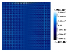
(a) T3 mesh: Error in LSB

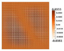
(b) T3 mesh: Lagrange multiplier enforcing LSB

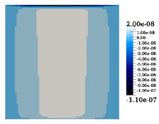
(c) Q4 mesh: Error in LSB

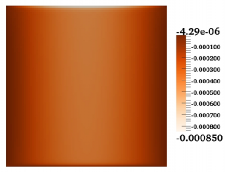
(d) Q4 mesh: Lagrange multiplier enforcing LSB

Figure 6. Numerical $h$-convergence study: The top and bottom left figures show the contours of error incurred in satisfying LSB for unconstrained negatively stabilized streamline diffusion LSFEM. The right set of figures show the contours of Lagrange multiplier enforcing LSB constraint using the proposed LSFEM. Note that the Lagrange multipliers enforcing the LSB constraint can have negative value as opposed to KKT multipliers. Numerical simulations are performed based on three-node triangular mesh and four-node quadrilateral mesh with 81 nodes on each side of the domain. In essence, the LSB errors and Lagrange multipliers enforcing LSB based on a Q4 mesh is lesser than a T3 mesh.

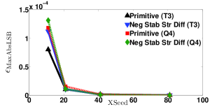
(a) LSB errors

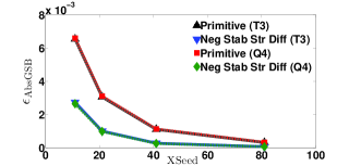
(b) GSB errors

Figure 7. Numerical $h$-convergence study: These figures show the decrease of $\epsilon_{\text{\tiny{MaxAbsLSB}}}$ and $\epsilon_{\text{\tiny{AbsGSB}}}$ with respect to XSeed for a series of hierarchical three-node triangular and four-node quadrilateral meshes. (See equations (4.15)–(4.17) for the definitions of $\epsilon_{\text{\tiny{MaxAbsLSB}}}$ and $\epsilon_{\text{\tiny{AbsGSB}}}$.) Numerical simulations are performed using the unconstrained primitive and negatively stabilized streamline diffusion LSFEMs. For XSeed = 81, $\epsilon_{\text{\tiny{MaxAbsLSB}}}$ and $\epsilon_{\text{\tiny{AbsGSB}}}$ are in $\mathcal{O}(10^{-6})$. In addition, the decrease in LSB and GSB errors with respect to $h$-refinement is slow, and the values are not close to the machine precision.

Another important aspect of this numerical $h$-convergence study is to quantify the errors incurred in satisfying LSB and GSB for unconstrained LSFEMs. The contours of the error distribution in LSB and the Lagrange multipliers enforcing the LSB constraints are shown in Figure 6. It is apparent that errors incurred in satisfying LSB are smaller under Q4 meshes than under T3 meshes. The decrease in $\epsilon_{\text{\tiny{MaxAbsLSB}}}$ and $\epsilon_{\text{\tiny{AbsGSB}}}$ on $h$-refinement is shown in Figure 7. From this figure, one can notice that the errors in LSB and GSB for a Q4 mesh are lesser than that of a T3 mesh. On $h$-refinement, the decrease in $\epsilon_{\text{\tiny{MaxAbsLSB}}}$ and $\epsilon_{\text{\tiny{AbsGSB}}}$ is slow and not close to machine precision.

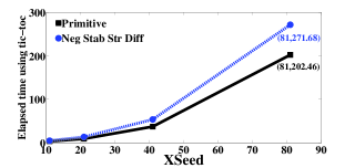
(a) T3 mesh

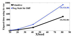
(b) Q4 mesh

Figure 8. Numerical $h$-convergence study: This figure shows the CPU time (in seconds) of the proposed computational framework for unconstrained primitive and unconstrained negatively stabilized streamline diffusion LSFEMs. For Q4 mesh, as $\mathrm{div}[\mathrm{grad}[c]]\neq 0$, the computational cost is higher than that of the T3 mesh.

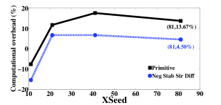
(a) T3 mesh

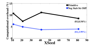
(b) Q4 mesh

Figure 9. Numerical $h$-convergence study: This figure shows the computational overhead incurred in satisfying LSB as compared to that of the corresponding unconstrained formulations. Analysis is performed for primitive and negatively stabilized streamline diffusion LSFEMs. For XSeed = 11, we obtained negative value for the computational overhead. This is because the interior point convex algorithm used in MATLAB optimization solver [33] pre-processes the constrained convex quadratic programming problem simplifies the given LSB constraints by removing redundancies. Hence, for very low number of unknowns, the computational cost associated with interior point convex algorithm is much faster than the LU solver for the unconstrained optimization problem.

Finally, the computational cost of the unconstrained and constrained LSFEMs for both T3 and Q4 meshes are shown in Figures 8 and 9. It is clear that the computational cost associated with a Q4 mesh is higher than that of a T3 mesh. This can be again be attributed to the non-vanishing stabilization terms (e.g., $\mathrm{div}[\mathrm{grad}[c(\mathbf{x})]$) in the negatively stabilized streamline diffusion LSFEM for Q4 meshes. For constrained LSFEMs, the maximum additional computational cost (for both LSFEMs) did not exceed $15\%$, which has been tested on a hierarchy of meshes.

5.2. Thermal boundary layer problem

This benchmark problem has wide practical applications in the areas of heat and mass transfer. Herein, we shall use this benchmark problem to study the performance of unconstrained and constrained LSFEM formulations in capturing steep gradients near the boundary for advection-dominated scenarios. Consider a rectangular domain $\Omega=\{(x,y)\in[0,1]\times[0,0.5]\}$ with velocity field $\mathbf{v}(x,y)=2y\mathbf{\hat{e}}_{x}$, where $\mathbf{\hat{e}}_{x}$ is the unit vector along the $x$-direction. The volumetric source is assumed to be homogeneous (i.e., $f(x,y)=0$), and the scalar diffusivity is taken to be $D(x,y)=10^{-4}$. The boundary conditions are:

$$c(x,y) =\begin{cases}0\quad\mathrm{for}\;0<x\leq 1\;\mathrm{and}\;y=0\\ 2y\;\;\;\mathrm{for}\;x=1\;\mathrm{and}\;0\leq y\leq 0.5\\ 1\quad\mathrm{for}\;0\leq x\leq 1\;\mathrm{and}\;y=1\\ 1\quad\mathrm{for}\;x=0\;\mathrm{and}\;0\leq y\leq 0.5\\ \end{cases}$$ (5.4)

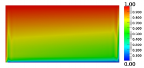
(a) Primitive (No constraints)

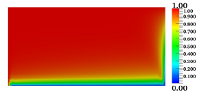
(b) Negatively stabilized streamline diffusion (LSB and NN constraints)

Figure 11. Thermal boundary layer problem: This figure shows the contours of concentration obtained for both unconstrained and constrained LSFEMs based on Q4 finite element mesh. The proposed LSFEM-based framework with NN and LSB constraints is able to eliminate spurious oscillations near the boundaries $y=0$ and $x=1$. This is not the case with the primitive LSFEM.

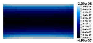
(a) Primitive

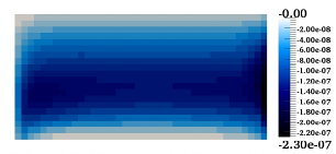
(b) Negatively stabilized streamline diffusion

Figure 12. Thermal boundary problem: This figure shows the contours of the error incurred in satisfying LSB for various unconstrained LSFEM formulations using Q4 meshes. One can notice that the error is more dominant in the interior of the domain under the primitive LSFEM, whereas the error is dominant at the boundary $x=1$ under the negatively stabilized streamline diffusion formulation.

A pictorial description of the boundary value problem is provided in Figure 10. The weights are taken to be that of LS Type-1 (see equations (4.6c) and (4.6f)). The element-level stabilization parameters for negatively stabilized streamline diffusion LSFEM are taken to be $\delta_{o}=0.01$ and $\tau_{o}=0.001$. Numerical simulations are performed using four-node quadrilateral mesh with XSeed = 41 and YSeed = 21. The element Péclet number will then be $\mathbb{P}\mathrm{e}_{h}=125$. The obtained concentration contours are shown in Figure 11. It is evident from these figures that numerical solution obtained from the primitive LSFEM contains node-to-node spurious oscillations. These oscillations did not reduce even after enforcing the LSB and NN constraints. But the negatively stabilized streamline diffusion LSFEM is able to capture the steep gradients near the boundary without producing spurious oscillations. The errors incurred in satisfying LSB for unconstrained LSFEM formulations are shown in Figure 12.

6. TRANSPORT-CONTROLLED BIMOLECULAR CHEMICAL REACTIONS

In this section, we shall apply the proposed mixed LSFEM-based computational framework to study transport-controlled bimolecular chemical reactions. Specifically, we are interested in the spatial distribution, plume formation, and chaotic mixing of chemical species at high Péclet numbers. To this end, consider the following irreversible bimolecular chemical reaction:

$$n_{A}\,A\,+\,n_{B}\,B\longrightarrow n_{C}\,C$$ (6.1)

where $A$, $B$, and $C$ are the species involved in the chemical reaction; $n_{A}$, $n_{B}$, and $n_{C}$ are their respective (positive) stoichiometric coefficients. The fate of these chemical species are governed by the following coupled advective-diffusive-reactive system:

$$\frac{\partial c_{A}}{\partial t}+\mathrm{div}[\mathbf{v}c_{A}-\mathbf{D}(\mathbf{x},t)\,\mathrm{grad}[c_{A}]]=f_{A}(\mathbf{x},t)-n_{\small{A}}\,r(\mathbf{x},t,c_{A},c_{B},c_{C})\quad\mathrm{in}\;\Omega\times]0,\mathcal{I}[$$ (6.2a)

$$\frac{\partial c_{B}}{\partial t}+\mathrm{div}[\mathbf{v}c_{B}-\mathbf{D}(\mathbf{x},t)\,\mathrm{grad}[c_{B}]]=f_{B}(\mathbf{x},t)-n_{\small{B}}\,r(\mathbf{x},t,c_{A},c_{B},c_{C})\quad\mathrm{in}\;\Omega\times]0,\mathcal{I}[$$ (6.2b)

$$\frac{\partial c_{C}}{\partial t}+\mathrm{div}[\mathbf{v}c_{C}-\mathbf{D}(\mathbf{x},t)\,\mathrm{grad}[c_{C}]]=f_{C}(\mathbf{x},t)+n_{\small{C}}\,r(\mathbf{x},t,c_{A},c_{B},c_{C})\quad\mathrm{in}\;\Omega\times]0,\mathcal{I}[$$ (6.2c)

$$c_{i}(\mathbf{x},t)=c^{\mathrm{p}}_{i}(\mathbf{x},t)\quad\mathrm{on}\;\Gamma^{c}_{i}\times]0,\mathcal{I}[$$ (6.2d)

$$\left(\left(\frac{1-\mathrm{Sign}[\mathbf{v}\bullet\widehat{\mathbf{n}}]}{2}\right)\mathbf{v}(\mathbf{x},t)c_{i}(\mathbf{x},t)-\mathbf{D}(\mathbf{x},t)\mathrm{grad}[c_{i}(\mathbf{x},t)]\right)\bullet\widehat{\mathbf{n}}(\mathbf{x})=h^{\mathrm{p}}_{i}(\mathbf{x},t)\quad\mathrm{on}\;\Gamma^{q}_{i}\times]0,\mathcal{I}[$$ (6.2e)

$$c_{i}(\mathbf{x},t=0)=c^{0}_{i}(\mathbf{x})\quad\mathrm{in}\;\Omega$$ (6.2f)

where $i=A,\,B$, and $C$. $\mathbf{v}(\mathbf{x},t)$ is the advection velocity vector field, $f_{i}(\mathbf{x},t)$ constitutes the non-reactive volumetric source, $c^{\mathrm{p}}_{i}(\mathbf{x},t)$ is the Dirichlet boundary condition, and $h^{\mathrm{p}}_{i}(\mathbf{x},t)$ is the Neumann boundary condition of the $i$-th chemical species. $r(\mathbf{x},t,c_{A},c_{B},c_{C})$ is the bimolecular chemical reaction rate, which is a non-linear function of the concentrations of the chemical species involved in the reaction. $c^{0}_{i}(\mathbf{x})$ is the initial condition of $i$-th chemical species. $t\in[0,\mathcal{I}]$ denote the time, where $\mathcal{I}$ is the total time of interest. The coupled governing equations (6.2a)–(6.2e) can be converted to a set of uncoupled advection-diffusion equations using the following linear algebraic transformation:

$$c_{F} :=c_{A}+\left(\frac{n_{A}}{n_{C}}\right)c_{C}$$ (6.3a)

$$c_{G} :=c_{B}+\left(\frac{n_{B}}{n_{C}}\right)c_{C}$$ (6.3b)

As we are interested in fast bimolecular chemical reactions, it is acceptable to assume that the chemical species $A$ and $B$ cannot co-exist at any given location $\mathbf{x}$ and time $t$. Hence, $c_{A}$, $c_{B}$, and $c_{C}$ can be evaluated as follows:

$$c_{A}(\mathbf{x},t)=\mathrm{max}\left[c_{F}(\mathbf{x},t)-\left(\frac{n_{A}}{n_{B}}\right)c_{G}(\mathbf{x},t),\,0\right]$$ (6.4a)

$$c_{B}(\mathbf{x},t)=\mathrm{max}\left[c_{G}(\mathbf{x},t)-\left(\frac{n_{B}}{n_{A}}\right)c_{F}(\mathbf{x},t),\,0\right]$$ (6.4b)

$$c_{C}(\mathbf{x},t)=\left(\frac{n_{C}}{n_{A}}\right)\;\big{(}c_{F}(\mathbf{x},t)-c_{A}(\mathbf{x},t)\big{)}$$ (6.4c)

In Reference [35], a similar mathematical model has been studied in the context of maximum principles and the non-negative constraint. However, the study has neglected the advection, and did not address local and global species balance. These aspects are very important and cannot be neglected in the numerical simulations of chemically reacting systems. In particular, advection can play a predominant role in the study of bioremediation [58], transverse mixing-controlled chemical reactions in hydro-geological media [59], and contaminant degradation problems [60]. This paper precisely addresses such problems in which advection is dominant, and satisfying species balance at both local and global levels is extremely important.

Remark 6.1.

Non-linear chemical dynamics is a huge field with various interesting artifacts, which include chaos and limit cycles [61, 62, 63]. Non-linear reactions will bring many additional complications, which need to be addressed systematically. Our approach can handle zeroth-order and first-order kinetics, as these two cases do not bring additional challenges. Other reaction kinetic models need to be addressed case-by-case. A general treatment of non-linear chemical dynamics is not trivial, and is beyond the scope of this paper.

Herein, we perform numerical simulations for highly spatially varying advection velocity fields and time-periodic flows. See Reference [61] for a discussion on time-periodic flows. For such problems in 2D, the following quantity is of considerable importance, which is referred as the position weighted second moment of the product $C$ concentration:

$$\Theta_{C}^{2}(t)=\frac{\displaystyle\int\limits_{\Omega}(y-y_{0})^{2}c_{C}(\mathbf{x},t)\;\mathrm{d}\Omega}{\displaystyle\int\limits_{\Omega}c_{C}(\mathbf{x},t)\;\mathrm{d}\Omega}$$ (6.5)

where $y_{0}$ is the location of a convenient reference horizontal line. In our numerical simulations, we have taken $y_{0}$ to be the $y$-coordinate of the start of the formation of product $C$. Since $c_{C}(\mathbf{x},t)\geq 0$, $\Theta^{2}_{C}(t)$ is a non-negative quantity. In subsequent sections, we study the utility of this quantity as a posteriori criterion to assess numerical accuracy. We also analyze the variation of $\Theta^{2}_{C}$ with respect to $\mathbb{P}\mathrm{e}_{h}$. We also present the numerical results that shed light on the impact of advection on the formation of the product $C$. In all our numerical simulations, we have taken the weights in primitive and negatively stabilized streamline diffusion LSFEMs to be that of LS Type-1 (i.e., $\mathbf{A}(\mathbf{x})=\mathbf{I}$ and $\beta(\mathbf{x})=1$).

Remark 6.2.

In the literature, to study mixing processes due to advection, spectral methods [64], pseudospectral methods [65], and model reduction methods [61] are commonly employed. However, such methods are limited to time-periodic flows, periodic initial and boundary conditions, simple geometries, and homogeneous isotropic diffusivity. Extending these methods to complicated geometries, general initial and boundary conditions, complicated advection velocity fields, and heterogeneous isotropic and anisotropic diffusivity is not trivial and may not even be possible. Moreover, these methods do not guarantee the satisfaction of non-negativity, DMPs, LSB, and GSB. The proposed computational framework is aimed at filling this lacuna.

6.1. One-dimensional steady-state analysis of product formation in fast reactions

Analysis is performed for two different advection velocities: $v=0.25$ and $v=1.0$. Diffusivity is assumed to be $2.5\times 10^{-3}$. The stoichiometric coefficients are assumed to be: $n_{A}=2$, $n_{B}=1$, and $n_{C}=1$. Numerical simulations are performed for two different cases as described below.

6.1.1. Case #1

A pictorial description of the boundary value problem is shown in Figure 13. The objective of this case study is to analyze whether the proposed negatively stabilized streamline diffusion LSFEM can produce physically meaningful values for $c_{i}(x)$ on coarse meshes. Based on the linear algebraic transformation given by equations (6.3a)–(6.3b), the analytical solution for invariants $F$ and $G$ can be written as follows:

$$c_{F}(x) =\left(1-\frac{1-\exp(vx/D)}{1-\exp(v/D)}\right)$$ (6.6a)

$$c_{G}(x) =\frac{f_{G}}{v}\left(x-\frac{1-\exp(vx/D)}{1-\exp(v/D)}\right)$$ (6.6b)

Using equations (6.4a)–(6.4c), one can obtain the analytical solution for product $C$.

For the numerical solution, we have taken XSeed = 11. The element stabilization parameters for negatively stabilized streamline diffusion LSFEM are taken as $\delta_{o}=0.08$ and $\tau_{o}=0.04$ when $v=0.25$. For $v=1.0$, $\delta_{o}$ and $\tau_{o}$, are assumed to equal to 0.083 and 0.0121, respectively. The analytical and numerical solutions are compared in Figure 14. As per this figure, the primitive LSFEM produces node-to-node oscillations near the boundaries of the domain. Furthermore, its numerical solution considerably deviates from the analytical solution in the entire domain. For $\mathbb{P}\mathrm{e}_{h}=5$ and $\mathbb{P}\mathrm{e}_{h}=20$, the negative value for the concentration is as low as $-1.25$ and $-0.47$. On the other hand, the negatively stabilized streamline diffusion LSFEM is able capture the analytical solution profile in the entire domain without producing negative values in the concentration field.

6.1.2. Case #2

A pictorial description of the boundary value problem is provided in Figure 13. The objective of this case study is to examine whether the proposed LSFEM can capture steep gradients in the solution near the boundary. The analytical solution for the invariants $F$ and $G$ can be written as follows:

$$c_{F}(x) =\left(1-\frac{1-\exp(vx/D)}{1-\exp(v/D)}\right)$$ (6.7a)

$$c_{G}(x) =\left(\frac{1-\exp(vx/D)}{1-\exp(v/D)}\right)$$ (6.7b)

Figure 15 compares the obtained the numerical solution with the analytical solution. The negatively stabilized streamline diffusion LSFEM is able to accurately capture the steep gradients near the boundary.

6.2. Steady-state plume formation from boundary in a reaction tank

A pictorial description of the boundary value problem is provided in Figure 16. The computational domain is a rectangle with $L_{x}=2$ and $L_{y}=1$. Dirichlet boundary conditions with $c^{\mathrm{p}}_{A}=c^{\mathrm{p}}_{B}=1$ are specified on the left side of the domain. Elsewhere, $c^{\mathrm{p}}_{i}(\mathbf{x})$ is taken to be zero for all the chemical species involved in the bimolecular reaction. The non-reactive volumetric source is assumed to be zero in the entire domain for all the chemical species. The stoichiometric coefficients are taken as $n_{A}=1$, $n_{B}=1$ and $n_{C}=1$. The advection velocity field is defined through the following multi-mode stream function [35]:

$$\psi(\mathbf{x}) =-\mathrm{y}-\sum_{k=1}^{3}A_{k}\cos\left(\frac{{p}_{k}\pi\mathrm{x}}{L_{x}}-\frac{\pi}{2}\right)\sin\left(\frac{q_{k}\pi\mathrm{y}}{L_{y}}\right)$$ (6.8)

where $\mathbf{x}=(x,y)$, $(p_{1},p_{2},p_{3})=(4,5,10)$, $(q_{1},q_{2},q_{3})=(1,5,10)$, and $(A_{1},A_{2},A_{3})=(0.08,0.02,0.01)$. The corresponding components of the advection velocity can be written as follows:

$$\mathrm{v}_{x}(\mathbf{x}) =-\frac{\partial\psi}{\partial\mathrm{y}}=1+\sum_{k=1}^{3}A_{k}\frac{q_{k}\pi}{L_{y}}\cos\left(\frac{p_{k}\pi\mathrm{x}}{L_{x}}-\frac{\pi}{2}\right)\cos\left(\frac{q_{k}\pi\mathrm{y}}{L_{y}}\right)$$ (6.9a)

$$\mathrm{v}_{y}(\mathbf{x}) =+\frac{\partial\psi}{\partial\mathrm{x}}=\sum_{k=1}^{3}A_{k}\frac{p_{k}\pi}{L_{x}}\sin\left(\frac{p_{k}\pi\mathrm{x}}{L_{x}}-\frac{\pi}{2}\right)\sin\left(\frac{q_{k}\pi\mathrm{y}}{L_{y}}\right)$$ (6.9b)

It is easy to check that $\mathrm{div}[\mathbf{v}(\mathbf{x})]=0$. The contours of the stream function and the corresponding advection velocity vector field are shown in Figure 16. Numerical simulations are performed using the following two different types of diffusivities:

• Type #1: $D(\mathbf{x})=10^{-2}$

• Type #2: $\mathbf{D}(\mathbf{x})=\mathbf{R}\mathbf{D}_{0}\mathbf{R}^{\mathrm{T}}$, where $\mathbf{R}$ and $\mathbf{D}_{0}$ are given as follows:

  $$\mathbf{R} =\left(\begin{array}[]{cc}\cos(\theta)&-\sin(\theta)\\ \sin(\theta)&\cos(\theta)\\ \end{array}\right)$$ (6.10c)

  $$\mathbf{D}_{0}(\mathbf{x}) =\omega_{0}\left(\begin{array}[]{cc}y^{2}_{*}+\omega_{2}x^{2}_{*}&-(1-\omega_{2})x_{*}y_{*}\\ -(1-\omega_{2})x_{*}y_{*}&\omega_{2}y^{2}_{*}+x^{2}_{*}\\ \end{array}\right)$$ (6.10f)

  where $x_{*}=x+\omega_{1}$ and $y_{*}=y+\omega_{1}$. The parameters $\theta$, $\omega_{0}$, $\omega_{1}$, and $\omega_{2}$ are equal to $\frac{\pi}{6}$, $1.0$, $10^{-3}$, and $10^{-3}$. Correspondingly, the eigenvalues of $\mathbf{D}(\mathbf{x})$ are $\omega_{0}(x^{2}_{*}+y^{2}_{*})$ and $\omega_{0}\omega_{2}\left(x^{2}_{*}+y^{2}_{*}\right)$. The contrast/anisotropic ratio of the media (which is the ratio of maximum to minimum eigenvalue) is as high as $10^{3}$.

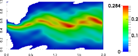
(a) $p=1$, XSeed = YSeed = 101

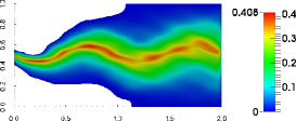
(b) $p=1$, XSeed = YSeed = 501

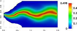
(c) $p=2$, XSeed = YSeed = 101

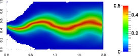
(d) $p=3$, XSeed = YSeed = 66

Figure 17. Plume development from boundary in a reaction tank (Type #1): This figure shows the concentration profiles of the product $C$ based on unconstrained primitive LSFEM. The white region shows the area in which concentration is negative. Both the lower-order and higher-order finite elements violate the non-negative constraint. The negative values are in the range $\mathcal{O}(10^{-2})$ to $\mathcal{O}(10^{-4})$, which are not close to the machine precision $\epsilon_{\mathrm{mach}}=\mathcal{O}(10^{-16})$.

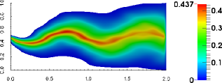
(a) XSeed = YSeed = 501 (No constraints)

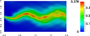
(b) XSeed = YSeed = 251 (NN constraints)

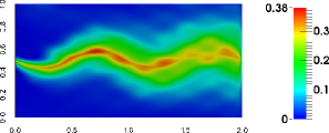
(c) XSeed = YSeed = 251 (LSB and NN constraints)

Figure 18. Plume development from boundary in a reaction tank (Type #1): This figure shows the concentration profiles of the product $C$ based on unconstrained and constrained negatively stabilized streamline diffusion LSFEM. The white region shows the area in which concentration is negative. Considerable part of the domain violated the non-negative constraint. The proposed framework with NN and LSB constraints is able to capture the plume formation on a coarse mesh for a highly heterogeneous advection velocity vector field.

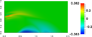
(a) XSeed = YSeed = 251 (No constraints)

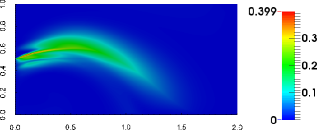
(b) XSeed = YSeed = 251 (NN constraints)

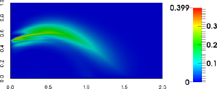
(c) XSeed = YSeed = 251 (LSB and NN constraints)

Figure 20. Plume development from boundary in a reaction tank (Type #2): This figure shows the concentration profiles of the product $C$ based on unconstrained and constrained negatively stabilized streamline diffusion LSFEM. Compared to Figure 19, the proposed methodology with NN and LSB constraints is able to accurately describe the plume formation of the product $C$ even for highly heterogeneous anisotropic diffusivities and highly spatially varying velocity fields.

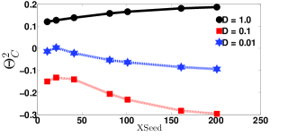
(a) No constraints

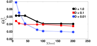
(b) With LSB and DMP constraints

Figure 21. Plume development from boundary in a reaction tank (Type #1): This figure shows the variation $\Theta_{C}^{2}$ with mesh refinement under the weighted negatively stabilized streamline diffusion LSFEM. It should be noted that $\Theta_{C}^{2}$ is a non-negative quantity. However, the unconstrained negatively stabilized streamline diffusion LSFEM gives negative values for $\Theta_{C}^{2}$. Mesh refinement did not alleviate this problem. On the other hand, the proposed framework not only gives non-negative values for $\Theta_{C}^{2}$ but flattens upon mesh refinement, which indicates convergence.

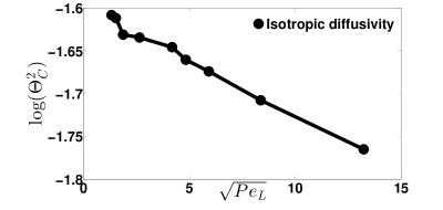
Figure 22. Plume development from boundary in a reaction tank (Type #1): This figure shows the variation $\log(\Theta^{2}_{C})$ with respect to $\sqrt{\mathbb{P}\mathrm{e}_{L}}$ for isotropic diffusivity under the weighted negatively stabilized streamline diffusion LSFEM with LSB and DMP constraints. Herein, analysis is performed using XSeed = YSeed = 201. Through numerical simulations, we observed that $\log(\Theta^{2}_{C})\propto\sqrt{\mathbb{P}\mathrm{e}_{L}}$.

Herein, we employed a structured mesh based on Q4 elements. Numerical simulations are performed with varying mesh sizes and polynomial orders ($p=1,2,3$) to demonstrate the pros and cons of various unconstrained and constrained LSFEMs. The stabilization parameters are taken as $\delta_{o}=\tau_{o}=10^{-3}$ and $\delta_{2}=\tau_{2}=10^{-4}$. The contours of the concentration of the product $C$ are shown in Figures 17–20 for both the primitive and negatively stabilized streamline diffusion LSFEMs. The white patches in the figures denote the regions in which the non-negative constraint has been violated. The variation of $\Theta^{2}_{C}$ with respect to XSeed and $Pe_{L}$ are shown in Figures 21–22. From these figures, the following inferences can be drawn:

1. It is clear that both low-order and higher-order polynomials violate the non-negative constraint and DMPs under unconstrained formulations. Moreover, mesh refinement and polynomial refinement do not seem to reduce the amount of violated region for DMP constraints.

2. The proposed framework based on $p=1$ is able to satisfy all the desired properties, and is able to predict physically meaningful values for the concentration and the flux.

3. The primitive LSFEM and the unconstrained negatively stabilized streamline diffusion LSFEM give unphysical values for the position weighted second moment of the product $C$ (i.e., $\Theta_{C}^{2}$). On the other hand, the proposed computational framework is able to accurately describe the variation of $\Theta_{C}^{2}$ with respect to mesh refinement. In addition, the numerical values for $\Theta_{C}^{2}$ reaches a plateau on $h$-refinement, which indicates convergence. However, this is not observed with the unconstrained primitive and negatively stabilized streamline diffusion LSFEMs.

Finally, it should be emphasized that placing explicit non-negative constraints on the nodal concentrations does not ensure non-negativity of the concentration in the entire computational domain. This is due to the fact that higher-order shape functions change their sign within an element [66].

6.3. Transient analysis of non-chaotic and chaotic vortex stirred mixing in a reaction tank

Figure 23 provides a pictorial description of the problem with appropriate initial and boundary conditions. The computational domain is a square with $L_{x}=L_{y}=1$. For all chemical species, zero flux boundary condition is prescribed on the entire boundary. The non-reactive volumetric source is zero in the entire domain for all the chemical species $A$, $B$, and $C$. Reactant $A$ is placed at the center of vortices, which are positioned at $(0.25,0.75)$ and $(0.75,0.25)$. The width of the square slug $A$ is equal to 0.25. Within this slug, $c_{A}(\mathbf{x},t=0)=8$. Elsewhere, the initial condition for $A$ is equal to zero. Correspondingly, the initial condition for reactant $B$ is zero in these two square regions centered at $(0.25,0.75)$ and $(0.75,0.25)$. Elsewhere, $c_{B}(\mathbf{x},t=0)=1.5$. The stoichiometric coefficients are taken as $n_{A}=1$, $n_{B}=1$, and $n_{C}=1$. The total time of interest is taken as $\mathcal{I}=5$. We assume scalar diffusivity to be $D=10^{-2}$. The stabilization parameters are taken as $\delta_{o}=\tau_{o}=10^{-3}$ and $\delta_{1}=\tau_{1}=10^{-4}$. For advection velocity, we employ the following vortex-based flow field:

• Type #1: Non-chaotic vortex-based advection velocity field

  $$\mathbf{v}(\mathbf{x})=\cos(2\pi y)\mathbf{\hat{e}}_{x}+\cos(2\pi x)\mathbf{\hat{e}}_{y}$$ (6.11)

• Type #2: Chaotic vortex-based advection velocity field

  $$\mathrm{v}_{x}(\mathbf{x},t)=\begin{cases}\cos(2\pi y)+v_{o}\sin(2\pi y)&\quad\mathrm{if}\;\nu T\leq t<\left(\nu+\frac{1}{2}\right)T\\ \cos(2\pi y)&\quad\mathrm{if}\;\left(\nu+\frac{1}{2}\right)T\leq t<\left(\nu+1\right)T\end{cases}$$ (6.12)

  $$\mathrm{v}_{y}(\mathbf{x},t)=\begin{cases}\cos(2\pi x)&\quad\mathrm{if}\;\nu T\leq t<\left(\nu+\frac{1}{2}\right)T\\ \cos(2\pi x)+v_{o}\sin(2\pi x)&\quad\mathrm{if}\;\left(\nu+\frac{1}{2}\right)T\leq t<\left(\nu+1\right)T\end{cases}$$ (6.13)

where $\nu=0,1,2,\cdots$ [64, 65]. $T$ denotes the period of the motion of the flow field. $v_{o}$ is an a-priorly chosen chaotic flow perturbation parameter. Herein, we choose $T=0.8$ and $v_{o}=1.0$ [67].

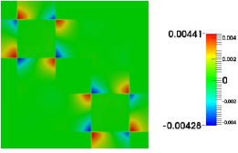
(a) Product $C$ at $t=0.0001$

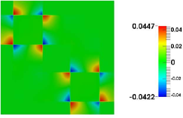
(b) Product $C$ at $t=0.001$

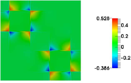
(c) Product $C$ at $t=0.01$

Figure 24. Non-chaotic vortex-stirred mixing in a reaction tank: This figure shows the concentration profiles of the product $C$ after the first time-step using the unconstrained weighted negatively stabilized streamline diffusion LSFEM. We have taken XSeed = YSeed = 121. If constraints are not enforced, one gets unphysical negative values for the concentration of product $C$. This will be particularly true in the early times of a numerical simulation.

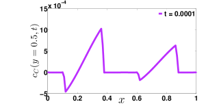
(a) $c_{C}(y=0.5,t=0.0001)$ with $\Delta t=0.0001$

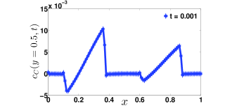
(b) $c_{C}(y=0.5,t=0.001)$ with $\Delta t=0.001$

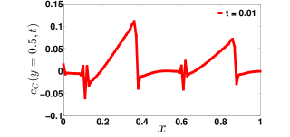
(c) $c_{C}(y=0.5,t=0.01)$ with $\Delta t=0.01$

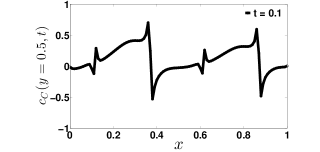
(d) $c_{C}(y=0.5,t=0.1)$ with $\Delta t=0.1$

Figure 25. Non-chaotic vortex-stirred mixing in a reaction tank: This figure shows the concentration profiles of the product $C$ at $y=0.5$ after the first time-step using the unconstrained weighted negatively stabilized streamline diffusion LSFEM. The violations of the non-negative constraint are significant, and are present for various choices of the time-step.

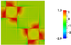
(a) Product $C$ at $t=0.1$ (No constraints)

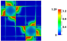
(b) Product $C$ at $t=0.1$ (NN constraints)

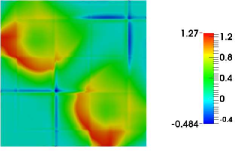
(c) Product $C$ at $t=0.5$ (No constraints)

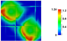
(d) Product $C$ at $t=0.5$ (NN constraints)

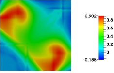
(e) Product $C$ at $t=1.0$ (No constraints)

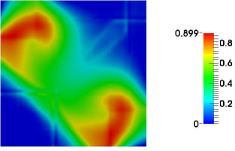
(f) Product $C$ at $t=1.0$ (NN constraints)

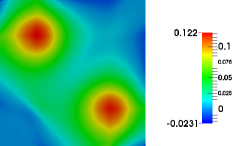
(g) Product $C$ at $t=5.0$ (No constraints)

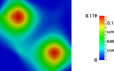
(h) Product $C$ at $t=5.0$ (NN constraints)

Figure 26. Non-chaotic vortex-stirred mixing in a reaction tank: This figure shows the concentration profiles of the product $C$ at various time levels using the weighted negatively stabilized streamline diffusion LSFEM with and without constraints. The time-step is taken as $\Delta t=0.1$. Herein, XSeed = YSeed = 121. As $t$ increases, the product $C$ should accumulate near the center of the two vortices. The proposed computational framework is able to accurately capture such features, and the obtained solutions are physical at all times.

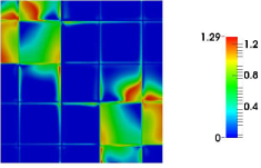
(a) Product $C$ at $t=0.1$

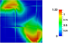
(b) Product $C$ at $t=0.5$

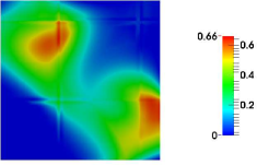
(c) Product $C$ at $t=1.0$

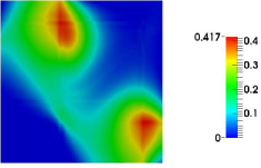
(d) Product $C$ at $t=1.5$

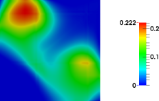
(e) Product $C$ at $t=2.0$

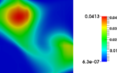
(f) Product $C$ at $t=3.0$

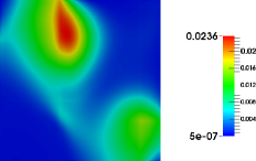
(g) Product $C$ at $t=4.0$

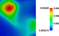
(h) Product $C$ at $t=5.0$

Figure 27. Chaotic vortex-stirred mixing in a reaction tank: This figure shows the concentration profiles of the product $C$ at various time levels using the proposed method with non-negative constraints. The time-step is taken as $\Delta t=0.1$. Herein, XSeed = YSeed = 121. An interesting feature observed is that the mixing of $c_{C}$ is enhanced in the entire domain when compared to non-chaotic advection (as the minimum value for $c_{C}$ is greater than zero).

Figures 24–27 provide the concentration profiles of unconstrained and constrained negatively stabilized streamline diffusion LSFEM with NN constraints. Herein, XSeed = YSeed = 121. Numerical simulations are performed for various different time steps. These are equal to 0.0001, 0.001, 0.01, and 0.1. Figure 24 shows the concentration profile of the product $C$ and Figure 25 shows the values of $c_{C}$ at $y=0.5$ at the first time-step. Analysis is performed using the unconstrained weighted negatively stabilized streamline diffusion LSFEM. From these figures, it is clear that unphysical negative values for $c_{C}$ are obtained even for small time steps. Furthermore, these violations are significant and not close to machine precision for both small and large time-steps. Non-negative constraints have to be enforced in order to get meaningful values for $c_{C}$.

Figures 26 and 27 show the concentration profiles of $c_{C}$ for both non-chaotic and chaotic vortex flow fields at various time levels. For non-chaotic advection, product $C$ is initially formed away from the vortex field. As time progresses, it slowly gets accumulated in the closed streamlines of the two vortices. Regions of higher concentration are located at the center of vortices. From Figure 26, it is evident that $c_{C}$ contour is symmetric along the line $y=x$. This is because the non-chaotic vortex-based advection velocity vector field is symmetric along this line. However, this is not the case with chaotic vortex flow field. Qualitatively, there is no symmetry associated with the concentration field. This is because of the time-periodic sinusoidal terms given by equations (6.12) and (6.13). They provide chaotic features for the chosen value of period of motion $T$. An interesting feature observed is that mixing of chemical species is enhanced in chaotic flow as compared to non-chaotic flow. This is because $c_{C}$ is not equal to zero in the non-chaotic flow for late times.

Finally, from these figures it is evident that existing numerical formulations do not provide accurate information on the fate of reactants and products for all times. On the other hand, the proposed methodology predicts results accurately for both early and late times.

6.4. Transient analysis of species mixing in cellular flows

A pictorial description of the initial boundary value problem is provided in Figure 28. The prescribed diffusive/total flux for each chemical species is taken to be equal to zero. The initial condition is such that $c^{0}_{A}(\mathbf{x})=1$ in the bottom half of the domain and vanishes elsewhere while $c^{0}_{B}(\mathbf{x})=1$ only in the upper half. The non-reactive part of the volumetric source is equal to zero for all the species. It should be noted that the concentration of the product $C$ should be between $0$ and $1$ because $f_{i}(\mathbf{x},t)=0$.

For numerical simulations, we have taken $L_{x}=1$, $L_{y}=0.5$, XSeed = 61 and YSeed = 241. The stoichiometric coefficients are taken as $n_{A}=1$, $n_{B}=1$, and $n_{C}=1$. The time-step is taken as $\Delta t=0.1$. The total time of interest is taken as $\mathcal{I}=5$. The scalar diffusivity is taken as $D=5\times 10^{-3}$. The stabilization parameters are taken as $\delta_{o}=\tau_{o}=10^{-3}$ and $\delta_{1}=\tau_{1}=10^{-4}$. The advection velocity vector field for the cellular flow is given by [68]:

$$\mathbf{v}(\mathbf{x}) =-\sin\left(\frac{2\pi x}{L_{\text{\tiny{Cell}}}}\right)\cos\left(\frac{2\pi y}{L_{\text{\tiny{Cell}}}}\right)\mathbf{\hat{e}}_{x}+\cos\left(\frac{2\pi x}{L_{\text{\tiny{Cell}}}}\right)\sin\left(\frac{2\pi y}{L_{\text{\tiny{Cell}}}}\right)\mathbf{\hat{e}}_{y}$$ (6.14)

where $L_{\text{\tiny{Cell}}}$ is the cell length of a pair of vortices. The velocity field given by equation (6.14) has a set of symmetrical vortices, and the neighboring vortices rotate in opposite directions. It is well-known that the advection velocity field given by equation (6.14) causes numerical difficulties (if the underlying numerical scheme is not properly designed). This is because the advection velocity is strongly non-uniform [68, Section 8], (which happens to be in our case). That is,

$$\mathop{\mathrm{max}}_{\mathbf{x}\in\overline{\Omega}}\left[\frac{\partial\mathrm{v}_{x}}{\partial x}-\frac{\partial\mathrm{v}_{y}}{\partial y}\right]\times\Delta t>1$$ (6.15)

The main objective of this test problem is show that the proposed formulation is robust and can analyze velocity fields that are strongly non-uniform without causing numerical instabilities/oscillations.

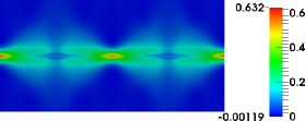
(a) Product $C$ at $t=0.1$ (No constraints)

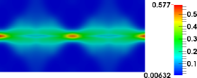
(b) Product $C$ at $t=0.1$ (LSB and DMP constraints)

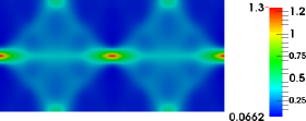
(c) Product $C$ at $t=0.5$ (No constraints)

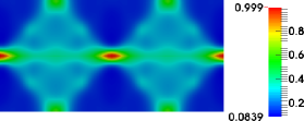
(d) Product $C$ at $t=0.5$ (LSB and DMP constraints)

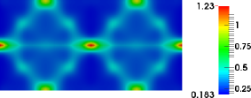
(e) Product $C$ at $t=1.0$ (No constraints)

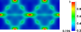
(f) Product $C$ at $t=1.0$ (LSB and DMP constraints)

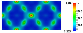
(g) Product $C$ at $t=5.0$ (No constraints)

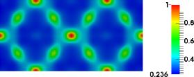
(h) Product $C$ at $t=5.0$ (LSB and DMP constraints)

Figure 29. Transport-controlled mixing in cellular flows: This figure shows the concentration profiles of the product $C$ at various time levels using the unconstrained and constrained weighted negatively stabilized streamline diffusion LSFEM when $L_{\text{\tiny{Cell}}}=0.5$. The proposed computational framework is able to produce physically meaningful solution (i.e., satisfies the non-negative constraint, maximum principle, and local species balance) for the product $C$ in a transient cellular flow. The time-step $\Delta t$ taken for the numerical simulation is equal to 0.1.

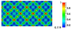
(a) Product $C$ for $L_{\text{\tiny{Cell}}}=0.25$

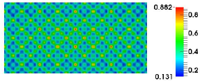
(b) Product $C$ for $L_{\text{\tiny{Cell}}}=0.125$

Figure 30. Transport-controlled mixing in cellular flows (with hierarchical cell lengths): This figure shows the concentration profiles of the product $C$ at $t=1$ using the proposed formulation with LSB and DMP constraints. Analysis is performed for a series of hierarchical $L_{\text{\tiny{Cell}}}$. The time-step $\Delta t$ is taken to be equal to 0.1.

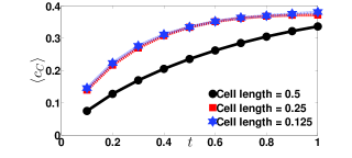
(a) $\langle c_{C}\rangle$ vs $t$

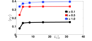
(b) $\langle c_{C}\rangle$ vs $L_{\text{\tiny{Cell}}}$

Figure 31. Transport-controlled mixing in cellular flows (with hierarchical cell lengths): This figure shows the average concentration of the product $C$ at various times and different cell lengths. Analysis is performed using the proposed formulation with LSB and DMP constraints. The time-step $\Delta t$ is taken to be equal to 0.1. The main inference from this numerical simulation is that species mixing happens faster as $L_{\text{\tiny{Cell}}}$ decreases.

Analysis is performed for a series of hierarchical cell lengths. That is $L_{\text{\tiny{Cell}}}$ equal to 0.5, 0.25, 0.125, 0.0625, and 0.03125. In all the cases, as the input data and the position of the cellular vortices is symmetric about the line $y=0.25$, it may be expected that formation of product $C$ will be symmetric along this line. Additional information on the symmetry of the formation of product $C$ can be inferred based on the cell length of adjacent pair of vortices, which rotate in opposite directions. This is apparent from the numerical results presented for product $C$ provided in Figures 29–31

Figure 29 shows the concentration profiles of the product $C$ under the unconstrained and constrained negatively stabilized streamline diffusion for $L_{\text{\tiny{Cell}}}=0.5$. From this figure, it is evident that the unconstrained LSFEM violates both the non-negative and maximum constraints. In addition, both undershoots and overshoots are observed. On the other hand, the proposed computational framework with LSB and DMP constraints provides physically meaningful profiles for the concentration of the product $C$.

For $L_{\text{\tiny{Cell}}}=0.5$, immediately after time $t=0$, we observe wing-like concentration profiles. This is because diffusion controls the species mixing rather than advection across the adjacent cells along the line $y=0.25$ (note that $\mathrm{v}_{y}(x,y=0.25)=0$). However, once the species $A$ and $B$ enter the closed streamlines where advection dominates, mixing happens at much faster rate. Furthermore, product $C$ spreads in time along the array of counter-rotating vortices. After a considerable time ($t\approx 5$), we observe that formation of product $C$ is symmetric along the lines $x=0.5$ and $y=0.25$. In addition, product $C$ accumulates near the region where $\|\mathbf{v}(\mathbf{x})\|$ is close to zero (which happens to be at the center of vortices and hyperbolic points). This happens to be in a good agreement with the inferences drawn from the numerical simulations performed on cellular flows [61, 68].

Figure 29 and 31 show that the separatrices connecting the hyperbolic points inhibit long range transport of chemical species from one cell to another. By decreasing $L_{\text{\tiny{Cell}}}$, species mixing can be enhanced. This is evident from Figure 31. Qualitatively, the numerical results presented here agree with the analysis presented by Neufeld and Garcia [61], which tells us that mixing of chemical species is fast within a cell but the transport of reactants/products between the cells is controlled by diffusion only. In order to enhance the efficient species mixing in different regions in these type of flows, $L_{\text{\tiny{Cell}}}$ has to be as smaller. To conclude, we would like to emphasize that the numerical solution based on the proposed methodology does not exhibit numerical instabilities and is able to capture the essential features even when the advection velocity is strongly non-uniform.

7. SUMMARY AND CONCLUDING REMARKS

We presented a robust computational framework for (steady-state and transient) advection-diffusion-reaction equations that satisfies the non-negative constraint, maximum principles, local species balance, and global species balance. The framework can handle general computational grids, anisotropic diffusivity, highly heterogeneous velocity fields, and provides physically meaningful numerical solutions without node-to-node spurious oscillations even on coarse computational meshes. The main contributions of the paper can be summarized as follows:

1. We constructed and proved a continuous maximum principle that includes both Dirichlet and Neumann boundary conditions. It also takes into account the inflow and outflow Neumann boundary conditions in establishing the maximum principle.

2. We described in detail the shortcomings of several plausible numerical approaches to satisfy the maximum principle, the non-negative constraint, and species balance.

3. We proposed a locally conservative DMP-preserving computational framework and constructed element stabilization parameters that are valid for a general reaction coefficient, advection velocity, and diffusivity. The framework has been carefully constructed using the least-squares finite element method (LSFEM). It is also shown that a naive implementation of LSFEM will not meet the desired properties.

4. The discrete problem under the proposed framework is well-posed, and it can be shown that a unique solution exists.

5. We performed numerical convergence studies on the computational framework. We also systematically analyzed and documented the performance of the proposed framework with various benchmark problems and realistic examples.

6. We obtained numerically a scaling law for a transport-controlled bimolecular reaction.

7. In chemically reactive systems, it is important to predict the fate of reactants and products during the early times. We have shown that the existing formulations may not provide accurate information for such scenarios. On the other hand, using numerical experiments, we have shown that the proposed framework predicts accurate results for both early and late times.

The salient features and performance of the proposed computational framework can be summarized as follows:

1. The rate of decrease of errors in LSB and GSB for unconstrained negatively stabilized streamline diffusion LSFEM with $h$-refinement is slow and is about $\mathcal{O}(h)$. Furthermore, this numerical formulation violates various discrete principles and the non-negative constraint for both isotropic and anisotropic diffusivities. On the other hand, the proposed non-negative computational framework is able to satisfy LSB and GSB up to machine precision on an arbitrary computational mesh.

2. The proposed computational framework with NN and LSB constraints eliminates the spurious node-to-node oscillations and provides physically meaningful values for concentration. Furthermore, it is able to furnish reasonable answers with various time-steps and at various time levels even on coarse computational grids.

3. It has been shown that existing formulations may fail to give acceptable results for non-negative statistical quantities such as $\Theta_{C}^{2}$, which is defined in Section 6.2. However, the proposed methodology always provides non-negative values for $\Theta_{C}^{2}$. The quantity $\Theta_{C}^{2}$ can be used as a posteriori criteria to assess accuracy of numerical solutions for complex initial and boundary value problems for which non-negativity and species conservation are important.

4. Due to the aforementioned desired properties, our proposed computational framework can be an ideal candidate to numerically obtain scaling laws for complicated problems with non-trivial initial and boundary conditions. Therefore, the proposed framework will be vital for predictive simulations in groundwater modeling, reactive transport, environmental fluid mechanics, and modeling of degradation of materials.

A possible future research work is to implement and analyze the performance of the proposed numerical methodology in a parallel environment. A related research is to design tailored iterative solvers and associated pre-conditioners for our proposed numerical methodology.

8. APPENDIX A: Element-level discretization of stabilization terms

The weighted negatively stabilized streamline diffusion least-squares formulation requires the evaluation of $\mathrm{div}[\mathrm{grad}[c(\mathbf{x})]]$ and $\mathrm{grad}[\mathrm{grad}[c(\mathbf{x})]]$ terms at the element-level. Since these terms are not typical, we present a compact way of discretizing these terms under the finite element method. It should be noted that one need not evaluate these terms for lowest-order simplicial elements (i.e., three-node triangular element and four-node tetrahedron element), as these terms will be identically zero. However, $\mathrm{div}[\mathrm{grad}[c(\mathbf{x})]]$ and $\mathrm{grad}[\mathrm{grad}[c(\mathbf{x})]]$ will be non-zero for high-order simplicial and non-simplicial elements (i.e., four-node quadrilateral element and eight-node brick element).

8.1. Fourth-order tensors

Let $\mathbf{R}$ and $\mathbf{S}$ be two second-order tensors. A fourth-order tensor product $\mathbf{R}\boxtimes\mathbf{S}$ is defined as follows:

$$\left(\mathbf{R}\boxtimes\mathbf{S}\right)\mathbf{T}=\mathbf{R}\mathbf{T}\mathbf{S}^{\mathrm{T}}$$ (8.1)

for any second-order tensor $\mathbf{T}$. The fourth-order identity tensor can then be written as:

$$\mathbb{I}=\mathbf{I}\boxtimes\mathbf{I}$$ (8.2)

where $\mathbf{I}$ is the second-order identity tensor. The fourth-order transposer $\mathbb{T}$ and symmetrizer $\mathbb{S}$ tensors are defined as follows:

$$\mathbb{T}\mathbf{A} =\mathbf{A}^{\mathrm{T}}$$ (8.3a)

$$\mathbb{S}\mathbf{A} =\frac{1}{2}\left(\mathbf{A}+\mathbf{A}^{\mathrm{T}}\right)$$ (8.3b)

where $\mathbf{A}$ is a general second-order tensor.

8.2. Properties of Kronecker products relevant to finite element discretization

Let $\boldsymbol{A}$ and $\boldsymbol{B}$ be matrices of sizes $n\times m$ and $p\times q$, respectively. Let $a_{ij}$ and $b_{ij}$ be, respectively, the $ij^{\mathrm{th}}$ components of $\boldsymbol{A}$ and $\boldsymbol{B}$. The Kronecker product of these two matrices is an $np\times mq$ matrix that is defined as follows:

$$\boldsymbol{A}\odot\boldsymbol{B}:=\left[\begin{array}[]{ccc}a_{11}\boldsymbol{B}&\ldots&a_{1m}\boldsymbol{B}\\ \vdots&\ddots&\vdots\\ a_{n1}\boldsymbol{B}&\ldots&a_{nm}\boldsymbol{B}\end{array}\right]$$ (8.7)

Another operator that will be useful is the $\mathrm{vec}[\bullet]$ operator, which is defined as follows:

$$\mathrm{vec}[\boldsymbol{A}]:=\left[\begin{array}[]{c}a_{11}\\ \vdots\\ a_{1m}\\ \vdots\\ a_{n1}\\ \vdots\\ a_{nm}\end{array}\right]$$ (8.15)

The following standard properties can be established for $\mathrm{mat}[\bullet]$ and $\mathrm{vec}[\bullet]$ operators:

$$\mathrm{vec}[\boldsymbol{A}+\boldsymbol{B}]=\mathrm{vec}[\boldsymbol{A}]+\mathrm{vec}[\boldsymbol{B}]$$ (8.16)

$$\left(\boldsymbol{A}\odot\boldsymbol{B}\right)\left(\boldsymbol{C}\odot\boldsymbol{D}\right)=\left(\boldsymbol{A}\boldsymbol{C}\odot\boldsymbol{B}\boldsymbol{D}\right)$$ (8.17)

$$\mathrm{vec}[\boldsymbol{ACB}]=\left(\boldsymbol{B}^{\mathrm{T}}\odot\boldsymbol{A}\right)\mathrm{vec}[\boldsymbol{C}]$$ (8.18)

For general properties of Kronecker products, see the book by Graham [69]. However, this book does not contain many of the results presented below, which are useful for the current study.

For an effective computer implementation of LSFEM-based formulations, we shall represent four-dimensional and three-dimensional arrays as two-dimensional matrices. To this end, consider a four-dimensional array $\boldsymbol{P}$ of size $m\times n\times p\times q$. The matrix representation of $\boldsymbol{P}$ is denoted by $\mathrm{mat}[\bullet]$, and is defined as follows:

$$\mathrm{mat}[\boldsymbol{P}] :=\left[\begin{array}[]{cccccc}P_{1111}&\ldots&P_{11p1}&P_{1112}&\ldots&P_{111q}\\ \vdots&\ddots&\vdots&\vdots&\ddots&\vdots\\ P_{mn11}&\ldots&P_{mnp1}&P_{mn12}&\ldots&P_{mnpq}\end{array}\right]$$ (8.22)

The following properties can be established for the matrix representation of fourth-order tensors:

$$\mathrm{vec}[\boldsymbol{P}\boldsymbol{X}]=\mathrm{mat}[\boldsymbol{P}]\mathrm{vec}[\boldsymbol{X}]$$ (8.23)

$$\mathrm{mat}[\boldsymbol{A}\boxtimes\boldsymbol{B}]=\boldsymbol{B}\odot\boldsymbol{A}$$ (8.24)

$$\mathrm{mat}[\mathbb{S}]=\frac{1}{2}\left(\boldsymbol{I}\odot\boldsymbol{I}+\mathrm{mat}[\mathbb{T}]\right)$$ (8.25)

where the matrix representation of $\mathbb{T}$ takes the following form:

$$\mathrm{mat}[\mathbb{T}]:=\left[\begin{array}[]{c}\boldsymbol{I}\odot[1,0,0,\ldots,0]_{n}\\ \boldsymbol{I}\odot[0,1,0,\ldots,0]_{n}\\ \vdots\\ \boldsymbol{I}\odot[0,0,0,\ldots,1]_{n}\end{array}\right]_{mn\times mn}$$ (8.30)

In the above equation, $\boldsymbol{I}$ is an identity matrix of size $m\times m$. It can be shown that for a matrix $\boldsymbol{Z}$ of size $m\times n$, $\mathrm{vec}[\boldsymbol{Z}^{\mathrm{T}}]=\mathrm{mat}[\mathbb{T}]\mathrm{vec}[\boldsymbol{Z}]$.

For a three-dimensional arrays, there are two useful matrix representations, which will be denoted as $\mathrm{mat}_{1}[\bullet]$ and $\mathrm{mat}_{2}[\bullet]$. Consider a three-dimensional array $\boldsymbol{Q}$ of size $m\times n\times p$. The corresponding matrix representations of $\boldsymbol{Q}$ are defined as follows:

$$\mathrm{mat}_{1}[\boldsymbol{Q}] :=\left[\begin{array}[]{cccccccc}Q_{111}&\ldots&Q_{1n1}&\ldots&\ldots&Q_{11p}&\ldots&Q_{1np}\\ \vdots&\ddots&\vdots&\vdots&\vdots&\vdots&\ddots&\vdots\\ Q_{m11}&\ldots&Q_{mn1}&\ldots&\ldots&Q_{m1p}&\ldots&Q_{mnp}\end{array}\right]$$ (8.34)

$$\mathrm{mat}_{2}[\boldsymbol{Q}] :=\left[\begin{array}[]{ccc}Q_{111}&\ldots&Q_{m11}\\ \vdots&\ddots&\vdots\\ Q_{11p}&\ldots&Q_{m1p}\\ Q_{121}&\ldots&Q_{m21}\\ \vdots&\ddots&\vdots\\ Q_{12p}&\ldots&Q_{m2p}\\ \vdots&\ddots&\vdots\\ Q_{1np}&\ldots&Q_{mnp}\end{array}\right]$$ (8.43)

The following properties can be established for the matrix representations of three-dimensional arrays:

$$\mathrm{vec}[\boldsymbol{Q}\boldsymbol{Y}]=\mathrm{mat}_{1}[\boldsymbol{Q}]\mathrm{vec}[\boldsymbol{Y}]$$ (8.44)

$$\mathrm{vec}[\boldsymbol{Q}\boldsymbol{z}]=\mathrm{mat}_{2}[\boldsymbol{Q}]\mathrm{vec}[\boldsymbol{z}]$$ (8.45)

8.3. Finite element discretization of $\mathrm{div}[\mathrm{grad}[c(\mathbf{x})]]$ and $\mathrm{grad}[\mathrm{grad}[c(\mathbf{x})]]$ terms

Let $\boldsymbol{\xi}$ denote the position vector in the reference finite element. The row vector containing the shape functions is denoted by $\boldsymbol{N}$, which is a function of $\boldsymbol{\xi}$. The derivatives and Hessian of $\boldsymbol{N}$ with respect to $\boldsymbol{\xi}$ are, respectively, denoted as $\boldsymbol{DN}$ and $\boldsymbol{DDN}$. That is, in indicial notation we have:

$$\left(\boldsymbol{DN}\right)_{ij}=\frac{\partial N_{i}}{\partial\xi_{j}}$$ (8.46a)

$$\left(\boldsymbol{DDN}\right)_{ijk}=\frac{\partial^{2}N_{i}}{\partial\xi_{j}\xi_{k}}$$ (8.46b)

where $N_{i}$ and $\xi_{i}$ are, respectively, the $i^{\mathrm{th}}$-component of the vectors $\boldsymbol{N}$ and $\boldsymbol{\xi}$. The concentration field $c(\mathbf{x})$ and total flux vector $\mathbf{q}(\mathbf{x})$ are interpolated as follows:

$$c(\mathbf{x}) =\widehat{\boldsymbol{c}}^{\mathrm{T}}\boldsymbol{N}^{\mathrm{T}}\left(\boldsymbol{\xi}(\boldsymbol{x})\right)$$ (8.47a)

$$\mathbf{q}(\mathbf{x}) =\widehat{\boldsymbol{q}}^{\mathrm{T}}\boldsymbol{N}^{\mathrm{T}}\left(\boldsymbol{\xi}(\boldsymbol{x})\right)$$ (8.47b)

where $\widehat{\boldsymbol{c}}^{\mathrm{T}}$ and $\widehat{\boldsymbol{q}}^{\mathrm{T}}$ denote the matrix containing nodal concentration and total flux vector. In negatively stabilized streamline diffusion LSFEM, $\mathrm{div}[\mathrm{grad}[c(\mathbf{x})]]$ and $\mathrm{grad}[\mathrm{grad}[c(\mathbf{x})]]$ terms arise from the following expansions:

$$\mathrm{div}[D(\mathbf{x})\mathrm{grad}[c(\mathbf{x})]] =\mathrm{grad}[D(\mathbf{x})]\bullet\mathrm{grad}[c(\mathbf{x})]+D(\mathbf{x})\,\mathrm{div}[\mathrm{grad}[c(\mathbf{x})]]$$ (8.48a)

$$\mathrm{div}[\mathbf{D}(\mathbf{x})\mathrm{grad}[c(\mathbf{x})]] =\mathrm{div}[\mathbf{D}(\mathbf{x})]\bullet\mathrm{grad}[c(\mathbf{x})]+\mathbf{D}(\mathbf{x})\bullet\mathrm{grad}[\mathrm{grad}[c(\mathbf{x})]]$$ (8.48b)

Based on the regularity of diffusivity, $\mathrm{grad}[D(\mathbf{x})]$ and $\mathrm{div}[\mathbf{D}(\mathbf{x})]$ can be calculated in multiple ways. If the diffusivity is continuously differentiable, then $\mathrm{grad}[D(\mathbf{x})]$ and $\mathrm{div}[\mathbf{D}(\mathbf{x})]$ can be directly evaluated analytically. This will considerably reduce the computational cost in the evaluation of local stiffness matrices. If $D(\mathbf{x})$ is not differentiable (but is square integrable), then $\mathrm{grad}[D(\mathbf{x})]$ and $\mathrm{div}[\mathbf{D}(\mathbf{x})]$ can be evaluated as follows:

$$\mathrm{grad}[D(\mathbf{x})] =\widehat{\boldsymbol{D}}^{\mathrm{T}}(\boldsymbol{DN})\boldsymbol{J}^{-1}$$ (8.49a)

$$\mathrm{div}[\mathbf{D}(\mathbf{x})] =\mathrm{mat}_{1}[\widehat{\boldsymbol{D}}]\mathrm{vec}[\mathrm{mat}[\mathbb{T}](\boldsymbol{DN})\boldsymbol{J}^{-1}]$$ (8.49b)

where $\boldsymbol{J}$ is the Jacobian matrix, and $\widehat{\boldsymbol{D}}$ is the nodal values for the diffusivity, whose size can be inferred based on the context (whether the diffusivity is either $D(\mathbf{x})$ or $\mathbf{D}(\mathbf{x})$). Using equations (8.46) and (8.47), the Laplacian and Hessian of $c(\mathbf{x})$ can be calculated as follows:

$$\mathrm{div}[\mathrm{grad}[c(\mathbf{x})]] =\Bigg{(}\left(\boldsymbol{I}-(\boldsymbol{DN})\boldsymbol{J}^{-1}\widehat{\boldsymbol{x}}^{\mathrm{T}}\right)\mathrm{mat}_{1}[\boldsymbol{DDN}]\mathrm{vec}[\boldsymbol{J}^{-1}\boldsymbol{J}^{-\mathrm{T}}]\Bigg{)}^{\mathrm{T}}\mathrm{vec}[\widehat{\boldsymbol{c}}^{\mathrm{T}}]$$ (8.50)

$$\mathrm{vec}[\mathrm{grad}[\mathrm{grad}[c(\mathbf{x})]]] =\Bigg{(}\left(\boldsymbol{J}^{-\mathrm{T}}\odot\boldsymbol{J}^{-\mathrm{T}}\right)\mathrm{mat}_{2}[\boldsymbol{DDN}]\left(\boldsymbol{I}\odot\boldsymbol{I}-\widehat{\boldsymbol{x}}\boldsymbol{J}^{\mathrm{T}}(\boldsymbol{DN})^{\mathrm{T}}\right)\Bigg{)}\mathrm{vec}[\widehat{\boldsymbol{c}}^{\mathrm{T}}]$$ (8.51)

where $\widehat{\boldsymbol{x}}$ is the matrix containing nodal coordinates.

9. APPENDIX B: Coercivity, error estimates, and stabilization parameters

Herein, we shall establish coercivity and error estimates for the homogeneous weighted LSFEMs (i.e., $c^{\mathrm{p}}(\mathbf{x})=0$ on $\partial\Omega$). Based on this mathematical analysis, we obtain the stabilization parameters that are used in this paper for the weighted negatively stabilized streamline diffusion LSFEM. To this end, let $H^{m}(\Omega)$ denote the standard Sobolev space for a given non-negative integer $m$ [28]. The associated standard inner product and norm are denoted by $(\bullet;\bullet)_{m}$ and $\|\bullet\|_{m}$, respectively. On the function space $\mathcal{Q}$, the inner product $(\bullet;\bullet)_{\mathrm{div}}$ and norm $\|\bullet\|_{\mathrm{div}}$ are defined as follows:

$$(\mathbf{p};\mathbf{q})_{\mathrm{div}} :=(\mathbf{p};\mathbf{q})_{0}+(\mathrm{div}[\mathbf{p}];\mathrm{div}[\mathbf{q}])_{0}\quad\forall\mathbf{p},\mathbf{q}\in\mathcal{Q}$$ (9.1a)

$$\|\mathbf{p}\|^{2}_{\mathrm{div}} :=\|\mathbf{p}\|^{2}_{0}+\|\mathrm{div}[\mathbf{p}]\|^{2}_{0}\quad\forall\mathbf{p}\in\mathcal{Q}$$ (9.1b)

The Poincaré-Friedrichs inequality takes the following form [45]: there exists a constant $C_{pf}>0$ such that we have

$$\|u\|_{0}\leq C_{pf}\|\mathrm{grad}[u]\|_{0}\quad\forall\,u\in H^{1}_{0}(\Omega)$$ (9.2)

Consider the classical weighted primitive least-squares functional $\mathfrak{F}_{\mathrm{Prim}}\left(\left(c,\mathbf{q}\right),f\right)$ given by equation (4.2) with $c(\mathbf{x})=0$ on $\partial\Omega$. If $(c,\mathbf{q})\in\mathcal{C}\times\mathcal{Q}$ is an exact solution of the equations (2.1a)–(2.1c), then $(c,\mathbf{q})$ must be a unique zero minimizer of $\mathfrak{F}_{\mathrm{Prim}}\left(\left(c,\mathbf{q}\right),f\right)$ on $\mathcal{C}\times\mathcal{Q}$. Hence, for any $\epsilon\in\mathbb{R}$, we have

$$\frac{d}{d\epsilon}\mathfrak{F}_{\mathrm{Prim}}\left(\left(c,\mathbf{q}\right)+\epsilon\left(w,\mathbf{p}\right),f\right)\Big{|}_{\epsilon=0}=0\quad\forall\left(w,\mathbf{p}\right)\in\mathcal{W}\times\mathcal{Q}$$ (9.3)

which is identical to the following:

$$\mathfrak{B}_{\mathrm{Prim}}\left(\left(c,\mathbf{q}\right);\left(w,\mathbf{p}\right)\right)=\mathfrak{L}_{\mathrm{Prim}}\left(\left(w,\mathbf{p}\right)\right)\quad\forall\left(w,\mathbf{p}\right)\in\mathcal{W}\times\mathcal{Q}$$ (9.4)

where $\mathfrak{B}_{\mathrm{Prim}}(\bullet;\bullet)$ and $\mathfrak{L}_{\mathrm{Prim}}(\bullet)$ are the corresponding bilinear and linear forms for the weighted primitive least-squares functional $\mathfrak{F}_{\mathrm{Prim}}$. It should be noted that

$$\mathfrak{B}_{\mathrm{Prim}}\left(\left(w,\mathbf{p}\right);\left(w,\mathbf{p}\right)\right)=\mathfrak{F}_{\mathrm{Prim}}\left(\left(w,\mathbf{p}\right),f=0\right)\quad\forall\left(w,\mathbf{p}\right)\in\mathcal{W}\times\mathcal{Q}$$ (9.5)

Equation (9.5) is used to prove coercivity and boundedness estimates for the bilinear form $\mathfrak{B}_{\mathrm{Prim}}$. Now consider the finite element discretization of the equation (9.4). Let $\mathcal{C}_{h}\subseteq\mathcal{C}$, $\mathcal{W}_{h}\subseteq\mathcal{W}$, and $\mathcal{Q}_{h}\subseteq\mathcal{Q}$ be the finite element function spaces spanned by piecewise polynomials of degree less than or equal to $r$ over $\Omega_{h}$. It should be noted that $r$ is an integer and $r\geq 1$. Then, the discrete weighted primitive LSFEM can be written as follows: Find $\left(c_{h},\mathbf{q}_{h}\right)\in\mathcal{C}_{h}\times\mathcal{Q}_{h}$ such that

$$\mathfrak{B}_{\mathrm{Prim}}\left(\left(c_{h},\mathbf{q}_{h}\right);\left(w_{h},\mathbf{p}_{h}\right)\right)=\mathfrak{L}_{\mathrm{Prim}}\left(\left(w_{h},\mathbf{p}_{h}\right)\right)\quad\forall\left(w_{h},\mathbf{p}_{h}\right)\in\mathcal{W}_{h}\times\mathcal{Q}_{h}$$ (9.6)

where $\left(c_{h},\mathbf{q}_{h}\right)$ is the finite element solution with respect to the chosen basis functions spanning the finite element space $\mathcal{C}_{h}\times\mathcal{Q}_{h}$. Similar inference holds for $\mathfrak{F}_{\mathrm{NgStb}}((c,\mathbf{q}),f)$, $\mathfrak{B}_{\mathrm{NgStb}}$, and $\mathfrak{L}_{\mathrm{NgStb}}$.

We assume that $\Omega_{h}$ is quasi-uniform [46, 45]. That is, there exists a constant $\widehat{C}>0$ independent of $h$ such that $h\leq\widehat{C}h_{\Omega_{e}}$ for all $\Omega_{e}\in\Omega_{h}$. Additionally, we assume that the following inverse inequality holds on these quasi-uniform meshes. There exists a constant $\widetilde{C}>0$ independent of $h$ such that

$$\widetilde{C}\sum_{\Omega_{\mathrm{e}}\in\Omega_{h}}h^{2}_{\Omega_{e}}\Big{\|}\mathrm{div}[\mathrm{grad}[c_{h}]]\Big{\|}^{2}_{0,\Omega_{e}}\leq\|\mathrm{grad}[c_{h}]\|^{2}_{0}\quad\forall c_{h}\in\mathcal{C}_{h}$$ (9.7a)

$$\Big{\|}\mathbf{D}\bullet\mathrm{grad}[\mathrm{grad}[c_{h}]]\Big{\|}_{0} \leq\Big{\|}\mathrm{tr}[\mathbf{D}]\mathrm{tr}[\mathrm{grad}[\mathrm{grad}[c_{h}]]]\Big{\|}_{0}=\mathrm{tr}[\mathbf{D}]\Big{\|}\mathrm{div}[\mathrm{grad}[c_{h}]]\Big{\|}_{0}\quad\forall c_{h}\in\mathcal{C}_{h}$$ (9.7b)

where $\mathrm{tr}[\bullet]$ is the trace of a matrix. In proposing equation (9.7b), we assumed that the Hessian of $c_{h}$, $\mathrm{grad}[\mathrm{grad}[c_{h}]]$, is positive semi-definite.

All the results presented here are applicable for a general anisotropic diffusivity tensor, advection velocity vector field, and linear reaction coefficient. One can obtain simplified results for isotropy by taking $\mathbf{D}(\mathbf{x})=D(\mathbf{x})\mathbf{I}$, where $\mathbf{I}$ is an identity tensor.

Theorem 9.1 (Coercivity for weighted primitive LSFEM).

There exist constants $C_{\mathrm{Prim}1}>0$ and $C_{\mathrm{Prim}2}>0$ independent of $\mathbf{D}$ and $h$ such that for all $\left(w_{h},\mathbf{p}_{h}\right)\in\mathcal{W}_{h}\times\mathcal{Q}_{h}$:

$$\mathfrak{F}_{\mathrm{Prim}}\left(\left(w_{h},\mathbf{p}_{h}\right),f=0\right) \geq C_{\mathrm{Prim}1}\gamma^{2}_{\mathrm{min}}\lambda^{2}_{\mathrm{min}}\|\mathrm{grad}[w_{h}]\|^{2}_{0}$$ (9.8a)

$$\mathfrak{F}_{\mathrm{Prim}}\left(\left(w_{h},\mathbf{p}_{h}\right),f=0\right) \geq C_{\mathrm{Prim}2}\gamma^{2}_{\mathrm{min}}\lambda^{2}_{\mathrm{min}}\left(\|w_{h}\|^{2}_{1}+\frac{\|\mathbf{p}_{h}\|^{2}_{\mathrm{div}}}{1+\lambda^{2}_{\mathrm{min}}+\lambda^{2}_{\mathrm{max}}}\right)$$ (9.8b)

where the positive constant $\gamma_{\mathrm{min}}$ is:

$$\gamma_{\mathrm{min}}:=\mathop{\mathrm{min}}\left[1,\mathop{\mathrm{min}}_{\mathbf{x}\in\overline{\Omega}}\left[\beta(\mathbf{x})\right],\mathop{\mathrm{min}}_{\mathbf{x}\in\overline{\Omega}}\left[\lambda_{\mathrm{\mathrm{min}},\mathbf{A}(\mathbf{x})}\right]\right]$$ (9.9)

where $\lambda_{\mathrm{\mathrm{min}},\mathbf{A}(\mathbf{x})}$ is the minimum eigenvalue of $\mathbf{A}(\mathbf{x})$ at a given point $\mathbf{x}\in\overline{\Omega}$.

Proof.

Consider the weighted primitive least-squares functional (4.2) with $f=0$. Equation (9.9) implies:

$$\frac{2\mathfrak{F}_{\mathrm{Prim}}}{\gamma^{2}_{\mathrm{min}}} \geq\Big{\|}\mathbf{p}_{h}-w_{h}\mathbf{v}+\mathbf{D}\mathrm{grad}[w_{h}]-\mu\mathrm{grad}[w_{h}]\Big{\|}^{2}_{0,\Omega}+\Big{\|}\alpha w_{h}+\mathrm{div}[\mathbf{p}_{h}]-\mu w_{h}\Big{\|}^{2}_{0,\Omega}$$

$$+2\mu\left(\mathbf{p}_{h}-w_{h}\mathbf{v}+\mathbf{D}\mathrm{grad}[w_{h}];\mathrm{grad}[w_{h}]\right)_{0,\Omega}+2\mu\left(\alpha w_{h}+\mathrm{div}[\mathbf{p}_{h}];w_{h}\right)_{0,\Omega}$$

$$-\mu^{2}\|w_{h}\|^{2}_{0,\Omega}-\mu^{2}\|\mathrm{grad}[w_{h}]\|^{2}_{0,\Omega}$$ (9.10)

where $\mu$ is a positive constant, which will be determined later. Using Poincaré-Friedrichs inequality and Green’s formulae, equation (9) can be written as:

$$\frac{2\mathfrak{F}_{\mathrm{Prim}}}{\gamma^{2}_{\mathrm{min}}} \geq\mu\left(2\lambda_{\mathrm{min}}-\mu\left(1+C^{2}_{pf}\right)\right)\|\mathrm{grad}[w_{h}]\|^{2}_{0,\Omega}$$ (9.11)

We obtain equation (9.8a) by choosing

$$\mu=\frac{\lambda_{\mathrm{min}}}{1+C^{2}_{pf}}$$ (9.12)

There exist two non-negative constants $C_{\mathbf{v}}$ and $C_{\alpha}$ (for instance, $C_{\mathbf{v}}=\displaystyle\mathop{\mathrm{max}}_{\mathbf{x}\in\overline{\Omega}}\left[\|\mathbf{v}\|^{2}\right]$ and $C_{\alpha}=\displaystyle\mathop{\mathrm{max}}_{\mathbf{x}\in\overline{\Omega}}\left[\alpha^{2}\right]$) such that

$$\|w_{h}\|^{2}_{1} =\|w_{h}\|^{2}_{0}+\|\mathrm{grad}[w_{h}]\|^{2}_{0}\leq\frac{2\left(1+C^{2}_{pf}\right)^{2}}{\gamma^{2}_{\mathrm{min}}\lambda^{2}_{\mathrm{min}}}\mathfrak{F}_{\mathrm{Prim}}$$ (9.13a)

$$\|\mathbf{p}_{h}\|^{2}_{0} \leq 2\|\mathbf{p}_{h}-w_{h}\mathbf{v}+\mathbf{D}\mathrm{grad}[w_{h}]\Big{\|}^{2}_{0,\Omega}+2\|-w_{h}\mathbf{v}+\mathbf{D}\mathrm{grad}[w_{h}]\Big{\|}^{2}_{0,\Omega}$$

$$\leq\left(1+\frac{2C_{\mathbf{v}}C^{2}_{pf}\left(1+C^{2}_{pf}\right)}{\lambda^{2}_{\mathrm{min}}}+2\left(1+C^{2}_{pf}\right)\frac{\lambda^{2}_{\mathrm{max}}}{\lambda^{2}_{\mathrm{min}}}\right)\frac{4\mathfrak{F}_{\mathrm{Prim}}}{\gamma^{2}_{\mathrm{min}}}$$ (9.13b)

$$\|\mathrm{div}[\mathbf{p}_{h}]\|^{2}_{0} \leq 2\big{\|}\alpha w_{h}+\mathrm{div}[\mathbf{p}_{h}]\big{\|}^{2}_{0,\Omega}+2\big{\|}\alpha w_{h}\big{\|}^{2}_{0,\Omega}\leq\left(1+\frac{C_{\alpha}C^{2}_{pf}\left(1+C^{2}_{pf}\right)}{\lambda^{2}_{\mathrm{min}}}\right)\frac{4\mathfrak{F}_{\mathrm{Prim}}}{\gamma^{2}_{\mathrm{min}}}$$ (9.13c)

It is easy to check that inequalities (9.13a)–(9.13c) imply inequality (9.8b). ∎

Theorem 9.2 (Coercivity and boundedness estimate for NSSD LSFEM).

Given that equations (9.7a)–(9.7b) hold. If for each $\Omega_{e}\in\Omega_{h}$ we take

$$\delta_{\Omega_{\mathrm{e}}} =-\frac{\widetilde{C}\lambda_{\mathrm{min}}h^{2}_{\Omega_{\mathrm{e}}}}{4\left(nd^{2}\lambda^{2}_{\mathrm{max}}+\widetilde{C}C^{2}_{pf}\delta_{\alpha\mathbf{v}}h^{2}+\widetilde{C}\delta_{\mathbf{D}}h^{2}\right)}$$ (9.14a)

$$\tau_{\Omega_{\mathrm{e}}} =-\frac{\widetilde{C}\lambda^{2}_{\mathrm{min}}h^{2}_{\Omega_{\mathrm{e}}}}{32\left(1+C^{2}_{pf}\right)\left(nd^{2}\lambda^{2}_{\mathrm{max}}+\widetilde{C}C^{2}_{pf}\delta_{\alpha\mathbf{v}}h^{2}+\widetilde{C}\delta_{\mathbf{D}}h^{2}\right)}$$ (9.14b)

then for all $\left(w_{h},\mathbf{p}_{h}\right)\in\mathcal{W}_{h}\times\mathcal{Q}_{h}$ there exist two constants $C_{\mathrm{NgStb}0}>0$ and $C_{\mathrm{NgStb}4}>0$ independent of $\mathbf{D}$ and $h$ such that we have:

Coercivity

$$\mathfrak{F}_{\mathrm{NgStb}}\left(\left(w_{h},\mathbf{p}_{h}\right),f=0\right) \geq\frac{11\gamma^{2}_{\mathrm{min}}\lambda^{2}_{\mathrm{min}}\|\mathrm{grad}[w_{h}]\|^{2}_{0}}{32(1+C^{2}_{pf})}$$

$$+\sum_{\Omega_{\mathrm{e}}\in\Omega_{h}}\frac{\widetilde{C}\gamma^{2}_{\mathrm{min}}\lambda^{2}_{\mathrm{min}}h^{2}_{\Omega_{\mathrm{e}}}\|\mathbf{v}\bullet\mathrm{grad}[w_{h}]\|^{2}_{0,\Omega_{\mathrm{e}}}}{32(1+C^{2}_{pf})\left(nd^{2}\lambda^{2}_{\mathrm{max}}+\widetilde{C}C^{2}_{pf}\delta_{\alpha\mathbf{v}}h^{2}+\widetilde{C}\delta_{\mathbf{D}}h^{2}\right)}$$ (9.15)

Boundedness estimate

$$C_{\mathrm{NgStb}1}\|w_{h}\|^{2}_{1}+C_{\mathrm{NgStb}2}\|\mathbf{p}_{h}\|^{2}_{\mathrm{div}} +C_{\mathrm{NgStb}3}\|\mathbf{v}\bullet\mathrm{grad}[w_{h}]\|^{2}_{0}\leq\mathfrak{F}_{\mathrm{NgStb}}\left(\left(w_{h},\mathbf{p}_{h}\right),f=0\right)$$

$$\leq C_{\mathrm{NgStb}4}\left(\|w_{h}\|^{2}_{1}+\|\mathbf{p}_{h}\|^{2}_{\mathrm{div}}+\|\mathbf{v}\bullet\mathrm{grad}[w_{h}]\|^{2}_{0}\right)$$ (9.16)

where the constant $\gamma_{\mathrm{min}}$ is given by equation (9.9). The constants $\delta_{\alpha\mathbf{v}}$, $\delta_{\mathbf{D}}$, $C_{\mathrm{NgStb}1}$, $C_{\mathrm{NgStb}2}$, and $C_{\mathrm{NgStb}2}$ are given as follows:

$$\delta_{\alpha\mathbf{v}} =\displaystyle\mathop{\mathrm{max}}_{\mathbf{x}\in\overline{\Omega}}\left[\left(\alpha+\mathrm{div}[\mathbf{v}]\right)^{2}\right]$$ (9.17a)

$$\delta_{\mathbf{D}} =\displaystyle\mathop{\mathrm{max}}_{\mathbf{x}\in\overline{\Omega}}\left[\|\mathrm{div}[\mathbf{D}]\|^{2}\right]$$ (9.17b)

$$C_{\mathrm{NgStb}1} =C_{\mathrm{NgStb}0}\gamma^{2}_{\mathrm{min}}\lambda^{2}_{\mathrm{min}}$$ (9.17c)

$$C_{\mathrm{NgStb}2} =\frac{C_{\mathrm{NgStb}0}\gamma^{2}_{\mathrm{min}}\lambda^{2}_{\mathrm{min}}\delta^{2}_{\alpha\mathbf{v}\mathbf{D}}}{\left(1+\lambda^{2}_{\mathrm{min}}+\lambda^{2}_{\mathrm{max}}\right)\delta^{2}_{\alpha\mathbf{v}\mathbf{D}}+\delta_{\alpha\mathbf{v}\mathbf{D}}\lambda^{2}_{\mathrm{min}}h^{2}+\delta_{\alpha\mathbf{v}1}\lambda^{2}_{\mathrm{min}}h^{4}}$$ (9.17d)

$$C_{\mathrm{NgStb}3} =\frac{C_{\mathrm{NgStb}0}\gamma^{2}_{\mathrm{min}}\lambda^{2}_{\mathrm{min}}h^{2}}{\delta_{\alpha\mathbf{v}\mathbf{D}}}$$ (9.17e)

The constants $\delta_{\alpha\mathbf{v}1}$ and $\delta_{\alpha\mathbf{v}\mathbf{D}}$ in the above equations are defined as follows:

$$\delta_{\alpha\mathbf{v}1} =\displaystyle\mathop{\mathrm{max}}_{\mathbf{x}\in\overline{\Omega}}\left[\left(\mathrm{grad}[\alpha]\bullet\mathbf{v}+\alpha\mathrm{div}[\mathbf{v}]\right)^{2}\right]$$ (9.18a)

$$\delta_{\alpha\mathbf{v}\mathbf{D}} =\lambda^{2}_{\mathrm{max}}+\delta_{\alpha\mathbf{v}}h^{2}+\delta_{\mathbf{D}}h^{2}$$ (9.18b)

Proof.

The boundedness estimate is a direct consequence of the triangle inequality. Herein, we shall proceed to show the validity of coercivity estimates, specifically, equation (9.2) and the left hand side of (9.2). Let $\mu>0$ be a constant, which will be determined later. Using equation (9.9) and (4.3) with $f=0$, we have

$$\frac{2\mathfrak{F}_{\mathrm{NgStb}}}{\gamma^{2}_{\mathrm{min}}} \geq\sum_{\Omega_{\mathrm{e}}\in\Omega_{h}}\Big{\|}\mathbf{p}_{h}-w_{h}\mathbf{v}+\mathbf{D}\mathrm{grad}[w_{h}]-\delta_{\Omega_{\mathrm{e}}}\mathbf{v}\left(\mathrm{div}[w_{h}\mathbf{v}-\mathbf{D}\mathrm{grad}[w_{h}]]\right)-\mu\mathrm{grad}[w_{h}]\Big{\|}^{2}_{0,\Omega_{\mathrm{e}}}$$

$$+\sum_{\Omega_{\mathrm{e}}\in\Omega_{h}}\Big{\|}\alpha w_{h}+\mathrm{div}[\mathbf{p}_{h}]+\delta_{\Omega_{\mathrm{e}}}\mathrm{div}[\alpha w_{h}\mathbf{v}]-\mu w_{h}\Big{\|}^{2}_{0,\Omega_{\mathrm{e}}}-\mu^{2}\|w_{h}\|^{2}_{0,\Omega}-\mu^{2}\|\mathrm{grad}[w_{h}]\|^{2}_{0,\Omega}$$

$$+\sum_{\Omega_{\mathrm{e}}\in\Omega_{h}}\tau_{\Omega_{\mathrm{e}}}\Big{\|}\alpha w_{h}+\mathrm{div}\big{[}w_{h}\mathbf{v}-\mathbf{D}\mathrm{grad}[w_{h}]\big{]}\Big{\|}^{2}_{0,\Omega_{\mathrm{e}}}+\sum_{\Omega_{\mathrm{e}}\in\Omega_{h}}2\mu\left(\alpha w_{h}+\mathrm{div}[\mathbf{p}_{h}+\delta_{\Omega_{\mathrm{e}}}\alpha w_{h}\mathbf{v}];w_{h}\right)_{0,\Omega}$$

$$+\sum_{\Omega_{\mathrm{e}}\in\Omega_{h}}2\mu\left(\mathbf{p}_{h}-w_{h}\mathbf{v}+\mathbf{D}\mathrm{grad}[w_{h}]-\delta_{\Omega_{\mathrm{e}}}\mathbf{v}\left(\mathrm{div}[w_{h}\mathbf{v}-\mathbf{D}\mathrm{grad}[w_{h}]]\right);\mathrm{grad}[w_{h}]\right)_{0,\Omega}$$ (9.19)

Using Theorem 9.1, equation (9.14a)–(9.14b), Cauchy-Schwartz inequality, Poincaré-Friedrichs inequality, Green’s formulae, and following inequalities

$$2\tau_{\Omega_{\mathrm{e}}}\left(\left(\alpha+\mathrm{div}[\mathbf{v}]\right)w_{h};\mathbf{v}\bullet\mathrm{grad}[w_{h}]\right)_{0,\Omega_{e}} \geq\tau_{\Omega_{\mathrm{e}}}\|\left(\alpha+\mathrm{div}[\mathbf{v}]\right)w_{h}\|^{2}_{0,\Omega_{e}}$$

$$+\tau_{\Omega_{\mathrm{e}}}\|\mathbf{v}\bullet\mathrm{grad}[w_{h}]\|^{2}_{0,\Omega_{e}}$$ (9.20a)

$$-2\tau_{\Omega_{\mathrm{e}}}\left(\left(\alpha+\mathrm{div}[\mathbf{v}]\right)w_{h};\mathbf{D}\bullet\mathrm{grad}[\mathrm{grad}[w_{h}]]\right)_{0,\Omega_{e}} \geq\tau_{\Omega_{\mathrm{e}}}\|\left(\alpha+\mathrm{div}[\mathbf{v}]\right)w_{h}\|^{2}_{0,\Omega_{e}}$$

$$+\tau_{\Omega_{\mathrm{e}}}\|\mathbf{D}\bullet\mathrm{grad}[\mathrm{grad}[w_{h}]]\|^{2}_{0,\Omega_{e}}$$ (9.20b)

$$-2\tau_{\Omega_{\mathrm{e}}}\left(\mathbf{v}\bullet\mathrm{grad}[w_{h}];\mathbf{D}\bullet\mathrm{grad}[\mathrm{grad}[w_{h}]]\right)_{0,\Omega_{e}} \geq\tau_{\Omega_{\mathrm{e}}}\|\mathbf{v}\bullet\mathrm{grad}[w_{h}]\|^{2}_{0,\Omega_{e}}$$

$$+\tau_{\Omega_{\mathrm{e}}}\|\mathbf{D}\bullet\mathrm{grad}[\mathrm{grad}[w_{h}]]\|^{2}_{0,\Omega_{e}}$$ (9.20c)

$$2\tau_{\Omega_{\mathrm{e}}}\left(\left(\alpha+\mathrm{div}[\mathbf{v}]\right)w_{h};\mathrm{div}[\mathbf{D}]\bullet\mathrm{grad}[w_{h}]\right)_{0,\Omega_{e}} \geq\tau_{\Omega_{\mathrm{e}}}\|\left(\alpha+\mathrm{div}[\mathbf{v}]\right)w_{h}\|^{2}_{0,\Omega_{e}}$$

$$+\tau_{\Omega_{\mathrm{e}}}\|\mathrm{div}[\mathbf{D}]\bullet\mathrm{grad}[w_{h}]\|^{2}_{0,\Omega_{e}}$$ (9.20d)

$$-2\tau_{\Omega_{\mathrm{e}}}\left(\mathrm{div}[\mathbf{D}]\bullet\mathrm{grad}[w_{h}];\mathbf{D}\bullet\mathrm{grad}[\mathrm{grad}[w_{h}]]\right)_{0,\Omega_{e}} \geq\tau_{\Omega_{\mathrm{e}}}\|\mathrm{div}[\mathbf{D}]\bullet\mathrm{grad}[w_{h}]\|^{2}_{0,\Omega_{e}}$$

$$+\tau_{\Omega_{\mathrm{e}}}\|\mathbf{D}\bullet\mathrm{grad}[\mathrm{grad}[w_{h}]]\|^{2}_{0,\Omega_{e}}$$ (9.20e)

$$2\tau_{\Omega_{\mathrm{e}}}\left(\mathbf{v}\bullet\mathrm{grad}[w_{h}];\mathrm{div}[\mathbf{D}]\bullet\mathrm{grad}[w_{h}]\right)_{0,\Omega_{e}} \geq\tau_{\Omega_{\mathrm{e}}}\|\mathbf{v}\bullet\mathrm{grad}[w_{h}]\|^{2}_{0,\Omega_{e}}$$

$$+\tau_{\Omega_{\mathrm{e}}}\|\mathrm{div}[\mathbf{D}]\bullet\mathrm{grad}[w_{h}]\|^{2}_{0,\Omega_{e}}$$ (9.20f)

we have the following inequality:

$$\sum_{\Omega_{\mathrm{e}}\in\Omega_{h}}\tau_{\Omega_{\mathrm{e}}}\Big{\|}\alpha w_{h}+\mathrm{div}\big{[}w_{h}\mathbf{v} -\mathbf{D}\mathrm{grad}[w_{h}]\big{]}\Big{\|}^{2}_{0,\Omega_{\mathrm{e}}}\geq-\frac{\lambda^{2}_{\mathrm{min}}}{16\left(1+C^{2}_{pf}\right)}$$

$$-\sum_{\Omega_{\mathrm{e}}\in\Omega_{h}}\frac{\widetilde{C}\lambda^{2}_{\mathrm{min}}h^{2}_{\Omega_{\mathrm{e}}}\|\mathbf{v}\bullet\mathrm{grad}[w_{h}]\|^{2}_{0,\Omega_{\mathrm{e}}}}{16(1+C^{2}_{pf})\left(nd^{2}\lambda^{2}_{\mathrm{max}}+\widetilde{C}C^{2}_{pf}\delta_{\alpha\mathbf{v}}h^{2}+\widetilde{C}\delta_{\mathbf{D}}h^{2}\right)}$$ (9.21)

Similarly, using the following equality:

$$2\mu\delta_{\Omega_{\mathrm{e}}}\left(\mathrm{div}[\alpha w_{h}\mathbf{v}];w_{h}\right)_{0,\Omega_{e}}=-2\mu\delta_{\Omega_{\mathrm{e}}}\left(\alpha w_{h};\mathbf{v}\bullet\mathrm{grad}[w_{h}]\right)_{0,\Omega_{e}}=\mu\delta_{\Omega_{\mathrm{e}}}\left(\mathrm{div}[\alpha\mathbf{v}]w_{h};w_{h}\right)_{0,\Omega_{e}}$$ (9.22)

in combination with the following inequalities

$$-2\mu\delta_{\Omega_{\mathrm{e}}}\left(\left(\alpha+\mathrm{div}[\mathbf{v}]\right)w_{h};\mathbf{v}\bullet\mathrm{grad}[w_{h}]\right)_{0,\Omega_{e}} \geq 2\mu\delta_{\Omega_{\mathrm{e}}}\|\left(\alpha+\mathrm{div}[\mathbf{v}]\right)w_{h}\|^{2}_{0,\Omega_{e}}$$

$$+\frac{\mu\delta_{\Omega_{\mathrm{e}}}}{2}\|\mathbf{v}\bullet\mathrm{grad}[w_{h}]\|^{2}_{0,\Omega_{e}}$$ (9.23a)

$$2\mu\delta_{\Omega_{\mathrm{e}}}\left(\mathrm{div}[\mathbf{D}]\bullet\mathrm{grad}[w_{h}];\mathbf{v}\bullet\mathrm{grad}[w_{h}]\right)_{0,\Omega_{e}} \geq 2\mu\delta_{\Omega_{\mathrm{e}}}\|\mathrm{div}[\mathbf{D}]\bullet\mathrm{grad}[w_{h}]\|^{2}_{0,\Omega_{e}}$$

$$+\frac{\mu\delta_{\Omega_{\mathrm{e}}}}{2}\|\mathbf{v}\bullet\mathrm{grad}[w_{h}]\|^{2}_{0,\Omega_{e}}$$ (9.23b)

$$2\mu\delta_{\Omega_{\mathrm{e}}}\left(\mathbf{D}\bullet\mathrm{grad}[\mathrm{grad}[w_{h}]];\mathbf{v}\bullet\mathrm{grad}[w_{h}]\right)_{0,\Omega_{e}} \geq 2\mu\delta_{\Omega_{\mathrm{e}}}\|\mathbf{D}\bullet\mathrm{grad}[\mathrm{grad}[w_{h}]]\|^{2}_{0,\Omega_{e}}$$

$$+\frac{\mu\delta_{\Omega_{\mathrm{e}}}}{2}\|\mathbf{v}\bullet\mathrm{grad}[w_{h}]\|^{2}_{0,\Omega_{e}}$$ (9.23c)

and choosing $\mu=\frac{\lambda_{\mathrm{min}}}{1+C^{2}_{pf}}$, equation (9) reduces to the following:

$$\frac{2\mathfrak{F}_{\mathrm{NgStb}}}{\gamma^{2}_{\mathrm{min}}} \geq\frac{3\lambda^{2}_{\mathrm{min}}}{4\left(1+C^{2}_{pf}\right)}+\sum_{\Omega_{\mathrm{e}}\in\Omega_{h}}\frac{\widetilde{C}\lambda^{2}_{\mathrm{min}}h^{2}_{\Omega_{\mathrm{e}}}\|\mathbf{v}\bullet\mathrm{grad}[w_{h}]\|^{2}_{0,\Omega_{\mathrm{e}}}}{8(1+C^{2}_{pf})\left(nd^{2}\lambda^{2}_{\mathrm{max}}+\widetilde{C}C^{2}_{pf}\delta_{\alpha\mathbf{v}}h^{2}+\widetilde{C}\delta_{\mathbf{D}}h^{2}\right)}$$

$$+\sum_{\Omega_{\mathrm{e}}\in\Omega_{h}}\tau_{\Omega_{\mathrm{e}}}\Big{\|}\alpha w_{h}+\mathrm{div}\big{[}w_{h}\mathbf{v}-\mathbf{D}\mathrm{grad}[w_{h}]\big{]}\Big{\|}^{2}_{0,\Omega_{\mathrm{e}}}$$ (9.24)

From equations (9) and (9.25a), we get the desired result given by equation (9.2). The second part of the proof is similar to Theorem 9.1. These exist a constant $C_{\alpha\mathbf{v}\mathbf{D}}>0$ (for instance, $C_{\alpha\mathbf{v}\mathbf{D}}=\displaystyle\mathop{\mathrm{max}}\left[nd^{2},\widetilde{C},\widetilde{C}C^{2}_{pf}\right]$) such that

$$nd^{2}\lambda^{2}_{\mathrm{max}}+\widetilde{C}C^{2}_{pf}\delta_{\alpha\mathbf{v}}h^{2}+\widetilde{C}\delta_{\mathbf{D}}h^{2} \leq C_{\alpha\mathbf{v}\mathbf{D}}\delta_{\alpha\mathbf{v}\mathbf{D}}$$ (9.25a)

$$\|\mathrm{grad}[w_{h}]\|^{2}_{0} \leq\frac{32(1+C^{2}_{pf})\mathfrak{F}_{\mathrm{NgStb}}}{11\gamma^{2}_{\mathrm{min}}\lambda^{2}_{\mathrm{min}}}$$ (9.25b)

$$\|\mathbf{v}\bullet\mathrm{grad}[w_{h}]\|^{2}_{0} \leq\frac{32C_{\alpha\mathbf{v}\mathbf{D}}\delta_{\alpha\mathbf{v}\mathbf{D}}(1+C^{2}_{pf})\widehat{C}^{2}\mathfrak{F}_{\mathrm{NgStb}}}{\widetilde{C}\gamma^{2}_{\mathrm{min}}\lambda^{2}_{\mathrm{min}}h^{2}}$$ (9.25c)

Using Cauchy-Schwartz inequality on $\|\mathbf{v}\bullet\mathrm{grad}[w_{h}]\|_{0}$ and (9.25b) gives

$$\|\mathbf{v}\bullet\mathrm{grad}[w_{h}]\|^{2}_{0}\leq\|\mathbf{v}\|^{2}_{0}\|\mathrm{grad}[w_{h}]\|^{2}_{0}\leq\frac{32C_{\mathbf{v}}(1+C^{2}_{pf})\mathfrak{F}_{\mathrm{NgStb}}}{11\gamma^{2}_{min}\lambda^{2}_{min}}$$ (9.26)

Now, consider the terms $\|w_{h}\|^{2}_{1}$ and $\|\mathbf{p}_{h}\|^{2}_{\mathrm{div}}$:

$$\|w_{h}\|^{2}_{1} =\|w_{h}\|^{2}_{0}+\|\mathrm{grad}[w_{h}]\|^{2}_{0}\leq\frac{32(1+C^{2}_{pf})^{2}\mathfrak{F}_{\mathrm{NgStb}}}{11\gamma^{2}_{min}\lambda^{2}_{min}}$$ (9.27a)

$$\|\mathbf{p}_{h}\|^{2}_{0} \leq 2\sum_{\Omega_{\mathrm{e}}\in\Omega_{h}}\Big{\|}\mathbf{p}_{h}-w_{h}\mathbf{v}+\mathbf{D}\mathrm{grad}[w_{h}]-\delta_{\Omega_{\mathrm{e}}}\mathbf{v}\left(\mathrm{div}[w_{h}\mathbf{v}-\mathbf{D}\mathrm{grad}[w_{h}]]\right)\Big{\|}^{2}_{0,\Omega_{\mathrm{e}}}$$

$$+2\sum_{\Omega_{\mathrm{e}}\in\Omega_{h}}\Big{\|}-w_{h}\mathbf{v}+\mathbf{D}\mathrm{grad}[w_{h}]-\delta_{\Omega_{\mathrm{e}}}\mathbf{v}\left(\mathrm{div}[w_{h}\mathbf{v}-\mathbf{D}\mathrm{grad}[w_{h}]]\right)\Big{\|}^{2}_{0,\Omega_{\mathrm{e}}}$$ (9.27b)

$$\|\mathrm{div}[\mathbf{p}_{h}]\|^{2}_{0} \leq 2\sum_{\Omega_{\mathrm{e}}\in\Omega_{h}}\Big{\|}\alpha w_{h}+\mathrm{div}[\mathbf{p}_{h}]+\delta_{\Omega_{\mathrm{e}}}\mathrm{div}[\alpha w_{h}\mathbf{v}]\Big{\|}^{2}_{0,\Omega_{\mathrm{e}}}$$

$$+2\sum_{\Omega_{\mathrm{e}}\in\Omega_{h}}\Big{\|}\alpha w_{h}+\delta_{\Omega_{\mathrm{e}}}\mathrm{div}[\alpha w_{h}\mathbf{v}]\Big{\|}^{2}_{0,\Omega_{\mathrm{e}}}$$ (9.27c)

Using (9.25a)–(9.26) and repeated use of triangle inequality on (9.27) and (9.27) gives the boundedness estimate (9.2). ∎

Theorem 9.3 (Error estimate for proposed LSFEM).

Given that equations (2.1a)–(2.1c) have a sufficiently smooth solution $\left(c,\mathbf{q}\right)\in\left(\mathcal{C}\times\mathcal{Q}\right)\cap\left(H^{r+1}(\Omega)\right)^{3}$. Then the finite element solution $\left(c_{h},\mathbf{q}_{h}\right)$ of the unconstrained weighted negatively stabilized streamline diffusion LSFEM satisfies the following error estimate:

$$\sqrt{C_{\mathrm{NgStb}1}}\|c-c_{h}\|_{1}+\sqrt{C_{\mathrm{NgStb}2}}\|\mathbf{q}-\mathbf{q}_{h}\|_{\mathrm{div}} +\sqrt{C_{\mathrm{NgStb}3}}\|\mathbf{v}\bullet\mathrm{grad}[c-c_{h}]\|_{0}$$

$$\leq C_{\mathrm{NgStb}}h^{r}\left(\|c\|_{r+1}+\|\mathbf{q}\|_{r+1}\right)$$ (9.28)

where $C_{\mathrm{NgStb}}>0$ is a constant independent of $\mathbf{D}$ and $h$.

Proof.

Let $c_{I}\in\mathcal{C}_{h}$ and $\mathbf{q}_{I}\in\mathcal{Q}_{h}$ be the standard finite element interpolants of $c$ and $\mathbf{q}$, respectively. From the interpolation theory [45], we have

$$\|c-c_{I}\|_{1} \leq Ch^{r}\|c\|_{r+1}$$ (9.29a)

$$\|\mathbf{q}-\mathbf{q}_{I}\|_{\mathrm{div}} \leq Ch^{r}\|\mathbf{q}\|_{r+1}$$ (9.29b)

for some positive constant $C$ independent of $\mathbf{D}$ and $h$. The error $\left(c-c_{h},\mathbf{q}-\mathbf{q}_{h}\right)$ satisfies the following orthogonality property:

$$\mathfrak{B}_{\mathrm{NgStb}}\left(\left(c_{h}-c,\mathbf{q}_{h}-\mathbf{q}\right);\left(w_{h},\mathbf{p}_{h}\right)\right)=0\quad\forall\left(w_{h},\mathbf{p}_{h}\right)\in\mathcal{W}_{h}\times\mathcal{Q}_{h}$$ (9.30)

Cauchy-Schwartz inequality implies:

$$\mathfrak{B}^{1/2}_{\mathrm{NgStb}}\left(\left(c_{h}-c_{I},\mathbf{q}_{h}-\mathbf{q}_{I}\right);\left(c_{h}-c_{I},\mathbf{q}_{h}-\mathbf{q}_{I}\right)\right)\leq\mathfrak{B}^{1/2}_{\mathrm{NgStb}}\left(\left(c-c_{I},\mathbf{q}-\mathbf{q}_{I}\right);\left(c-c_{I},\mathbf{q}-\mathbf{q}_{I}\right)\right)$$ (9.31)

From Theorem 9.2 and interpolation estimates (9.29a)–(9.29b), one can obtain the desired error estimate (9.3). ∎

From the above mathematical analysis, it is evident that the element-dependent stabilization parameters $\tau_{\Omega_{\mathrm{e}}}\leq 0$ and $\delta_{\Omega_{\mathrm{e}}}\leq 0$ can be taken as:

$$\delta_{\Omega_{\mathrm{e}}} =-\frac{\delta_{o}\lambda_{\mathrm{min}}h^{2}_{\Omega_{\mathrm{e}}}}{\left(\lambda^{2}_{\mathrm{max}}+\delta_{1}\displaystyle\mathop{\mathrm{max}}_{\mathbf{x}\in\overline{\Omega}}\left[\left(\alpha+\mathrm{div}[\mathbf{v}]\right)^{2}\right]h^{2}+\delta_{2}\displaystyle\mathop{\mathrm{max}}_{\mathbf{x}\in\overline{\Omega}}\left[\|\mathrm{div}[\mathbf{D}]\|^{2}\right]h^{2}\right)}$$ (9.32a)

$$\tau_{\Omega_{\mathrm{e}}} =-\frac{\tau_{o}\lambda^{2}_{\mathrm{min}}h^{2}_{\Omega_{\mathrm{e}}}}{\left(\lambda^{2}_{\mathrm{max}}+\tau_{1}\displaystyle\mathop{\mathrm{max}}_{\mathbf{x}\in\overline{\Omega}}\left[\left(\alpha+\mathrm{div}[\mathbf{v}]\right)^{2}\right]h^{2}+\tau_{2}\displaystyle\mathop{\mathrm{max}}_{\mathbf{x}\in\overline{\Omega}}\left[\|\mathrm{div}[\mathbf{D}]\|^{2}\right]h^{2}\right)}$$ (9.32b)

where $\delta_{o}$, $\delta_{1}$, $\delta_{2}$, $\tau_{o}$, $\tau_{1}$, and $\tau_{2}$ are non-negative constants.

Remark 9.4.

The mathematical analysis provided by Hsieh and Yang [14] can be obtained as a special case of the mathematical analysis presented above. Specifically, take $\alpha=0$, $\mathbf{D}(\mathbf{x})$ to be homogeneous and isotropic, and $\mathbf{v}(\mathbf{x})$ to be solenoidal and constant.

10. APPENDIX C: Finite element stiffness matrices and load vectors

For weighted primitive LSFEM the terms $\boldsymbol{K}_{cc}$, $\boldsymbol{K}_{c\mathbf{q}}$, $\boldsymbol{K}_{\mathbf{q}\mathbf{q}}$, $\boldsymbol{r}_{c}$, and $\boldsymbol{r}_{\mathbf{q}}$ are constructed from the local stiffness matrices and load vectors $\boldsymbol{K}^{e}_{cc}$, $\boldsymbol{K}^{e}_{c\mathbf{q}}$, $\boldsymbol{K}^{e}_{\mathbf{q}\mathbf{q}}$, $\boldsymbol{r}^{e}_{c}$, and $\boldsymbol{r}^{e}_{\mathbf{q}}$ through the standard finite element assembly process. The expressions for these element stiffness matrices and element load vectors in terms of shape functions and their derivatives are explicitly defined as follows:

$$\boldsymbol{K}^{e}_{cc} =\int\limits_{\Omega_{e}}\left(\beta^{2}\alpha^{2}\right)\boldsymbol{N}^{\mathrm{T}}\boldsymbol{N}\;\mathrm{d}\Omega_{e}\,+\,\int\limits_{\Omega_{e}}\boldsymbol{N}^{\mathrm{T}}\mathbf{v}^{\mathrm{T}}\mathbf{A}^{2}\mathbf{v}\boldsymbol{N}\;\mathrm{d}\Omega_{e}\,-\,\int\limits_{\Omega_{e}}\left(\boldsymbol{DN}\boldsymbol{J}^{-1}\right)\mathbf{D}\mathbf{A}^{2}\mathbf{v}\boldsymbol{N}\;\mathrm{d}\Omega_{e}$$

$$-\int\limits_{\Omega_{e}}\boldsymbol{N}^{\mathrm{T}}\mathbf{v}^{\mathrm{T}}\mathbf{A}^{2}\mathbf{D}\left(\boldsymbol{DN}\boldsymbol{J}^{-1}\right)^{\mathrm{T}}\;\mathrm{d}\Omega_{e}+\int\limits_{\Omega_{e}}\left(\boldsymbol{DN}\boldsymbol{J}^{-1}\right)\mathbf{D}\mathbf{A}^{2}\mathbf{D}\left(\boldsymbol{DN}\boldsymbol{J}^{-1}\right)^{\mathrm{T}}\;\mathrm{d}\Omega_{e}$$

$$+\int\limits_{\Omega_{\mathrm{e}}\in{\Gamma^{q}}}\left(\frac{1+\mathrm{Sign}[\mathbf{v}\bullet\widehat{\mathbf{n}}]}{2}\right)^{2}\left(\mathbf{v}\bullet\widehat{\mathbf{n}}\right)^{2}\boldsymbol{N}^{\mathrm{T}}\boldsymbol{N}\;\mathrm{d}\Gamma^{q}_{e}$$ (10.1)

$$\boldsymbol{K}^{e}_{c\mathbf{q}} =\int\limits_{\Omega_{e}}\left(\beta^{2}\alpha\right)\boldsymbol{N}^{\mathrm{T}}\left(\mathrm{vec}\left[\left(\boldsymbol{DN}\boldsymbol{J}^{-1}\right)^{\mathrm{T}}\right]\right)^{\mathrm{T}}\;\mathrm{d}\Omega_{e}\,-\,\int\limits_{\Omega_{e}}\boldsymbol{N}^{\mathrm{T}}\mathbf{v}^{\mathrm{T}}\mathbf{A}^{2}\left(\boldsymbol{N}\odot\boldsymbol{I}\right)\;\mathrm{d}\Omega_{e}$$

$$+\int\limits_{\Omega_{e}}\left(\boldsymbol{DN}\boldsymbol{J}^{-1}\right)\mathbf{D}\mathbf{A}^{2}\left(\boldsymbol{N}\odot\boldsymbol{I}\right)\;\mathrm{d}\Omega_{e}\,$$

$$-\,\int\limits_{\Omega_{\mathrm{e}}\in{\Gamma^{q}}}\left(\frac{1+\mathrm{Sign}[\mathbf{v}\bullet\widehat{\mathbf{n}}]}{2}\right)\left(\mathbf{v}\bullet\widehat{\mathbf{n}}\right)\boldsymbol{N}^{\mathrm{T}}\widehat{\mathbf{n}}^{\mathrm{T}}\left(\boldsymbol{N}\odot\boldsymbol{I}\right)\;\mathrm{d}\Gamma^{q}_{e}$$ (10.2)

$$\boldsymbol{K}^{e}_{\mathbf{q}\mathbf{q}} =\int\limits_{\Omega_{e}}\beta^{2}\left(\mathrm{vec}\left[\left(\boldsymbol{DN}\boldsymbol{J}^{-1}\right)^{\mathrm{T}}\right]\right)\left(\mathrm{vec}\left[\left(\boldsymbol{DN}\boldsymbol{J}^{-1}\right)^{\mathrm{T}}\right]\right)^{\mathrm{T}}\;\mathrm{d}\Omega_{e}\,+\,\int\limits_{\Omega_{e}}\left(\boldsymbol{N}^{\mathrm{T}}\odot\boldsymbol{I}\right)\mathbf{A}^{2}\left(\boldsymbol{N}\odot\boldsymbol{I}\right)\;\mathrm{d}\Omega_{e}$$

$$+\int\limits_{\Omega_{\mathrm{e}}\in{\Gamma^{q}}}\left(\boldsymbol{N}^{\mathrm{T}}\odot\boldsymbol{I}\right)\widehat{\mathbf{n}}\,\widehat{\mathbf{n}}^{\mathrm{T}}\left(\boldsymbol{N}\odot\boldsymbol{I}\right)\;\mathrm{d}\Gamma^{q}_{e}$$ (10.3)

Correspondingly, the expressions for the element load vectors in terms of shape functions and their derivatives are explicitly defined as follows:

$$\boldsymbol{r}^{e}_{c} =\int\limits_{\Omega_{e}}\left(\beta^{2}\alpha f\right)\boldsymbol{N}^{\mathrm{T}}\;\mathrm{d}\Omega_{e}\,-\,\int\limits_{\Omega_{\mathrm{e}}\in{\Gamma^{q}}}\left(\frac{1+\mathrm{Sign}[\mathbf{v}\bullet\widehat{\mathbf{n}}]}{2}\right)\left(\mathbf{v}\bullet\widehat{\mathbf{n}}\right)\boldsymbol{N}^{\mathrm{T}}q^{\mathrm{p}}\;\mathrm{d}\Gamma^{q}_{e}$$ (10.4)

$$\boldsymbol{r}^{e}_{\mathbf{q}} =\int\limits_{\Omega_{e}}\left(\beta^{2}f\right)\mathrm{vec}\left[\left(\boldsymbol{DN}\boldsymbol{J}^{-1}\right)^{\mathrm{T}}\right]\;\mathrm{d}\Omega_{e}\,+\,\int\limits_{\Omega_{\mathrm{e}}\in{\Gamma^{q}}}\left(\boldsymbol{N}^{\mathrm{T}}\odot\boldsymbol{I}\right)\widehat{\mathbf{n}}\,q^{\mathrm{p}}\;\mathrm{d}\Gamma^{q}_{e}$$ (10.5)

It should be noted that these terms are obtained from the bilinear and linear forms of the weighted primitive least-squares functional $\mathfrak{F}_{\mathrm{Prim}}$, which are given as follows:

$$\mathfrak{B}_{\mathrm{Prim}}\left(\left(c,\mathbf{q}\right);\left(w,\mathbf{p}\right)\right) =\left(w;\beta^{2}\alpha^{2}c\right)+\left(w;\left(\mathbf{v}\bullet\mathbf{A}^{2}\mathbf{v}\right)c\right)-\left(\mathrm{grad}[w];\left(\mathbf{D}A^{2}\mathbf{v}\right)c\right)$$

$$-\left(w;\mathbf{v}\bullet A^{2}\mathbf{D}\,\mathrm{grad}[c]\right)+\left(\mathrm{grad}[w];\left(\mathbf{D}A^{2}\mathbf{D}\right)\mathrm{grad}[c]\right)$$

$$+\left(w;\beta^{2}\alpha\,\mathrm{div}[\mathbf{q}]\right)+\left(\mathrm{div}[\mathbf{p}];\beta^{2}\alpha c\right)-\left(w;\mathbf{v}\bullet\mathbf{A}^{2}\mathbf{q}\right)-\left(\mathbf{p};\mathbf{A}^{2}\mathbf{v}c\right)$$

$$+\left(\mathrm{grad}[w];\mathbf{D}A^{2}\,\mathbf{q}\right)+\left(\mathbf{p};A^{2}\mathbf{D}\,\mathrm{grad}[c]\right)+\left(\mathrm{div}[\mathbf{p}];\beta^{2}\mathrm{div}[\mathbf{q}]\right)$$

$$+\left(\mathbf{p};A^{2}\mathbf{q}\right)+\left(w;\left(\frac{1+\mathrm{Sign}[\mathbf{v}\bullet\widehat{\mathbf{n}}]}{2}\right)^{2}\left(\mathbf{v}\bullet\widehat{\mathbf{n}}\right)^{2}\,c\right)_{\Gamma^{q}}$$

$$-\left(w;\left(\frac{1+\mathrm{Sign}[\mathbf{v}\bullet\widehat{\mathbf{n}}]}{2}\right)\left(\mathbf{v}\bullet\widehat{\mathbf{n}}\right)\,\mathbf{q}\bullet\widehat{\mathbf{n}}\right)_{\Gamma^{q}}+\left(\mathbf{p}\bullet\widehat{\mathbf{n}};\mathbf{q}\bullet\widehat{\mathbf{n}}\right)_{\Gamma^{q}}$$

$$-\left(\mathbf{p}\bullet\widehat{\mathbf{n}};\left(\frac{1+\mathrm{Sign}[\mathbf{v}\bullet\widehat{\mathbf{n}}]}{2}\right)\left(\mathbf{v}\bullet\widehat{\mathbf{n}}\right)c\right)_{\Gamma^{q}}$$ (10.6)

$$\mathfrak{L}_{\mathrm{Prim}}\left(\left(w,\mathbf{p}\right)\right) =\left(w;\beta^{2}\alpha f\right)+\left(\mathrm{div}[\mathbf{p}];\beta^{2}f\right)-\left(w;\left(\frac{1+\mathrm{Sign}[\mathbf{v}\bullet\widehat{\mathbf{n}}]}{2}\right)\left(\mathbf{v}\bullet\widehat{\mathbf{n}}\right)\;q^{\mathrm{p}}\right)_{\Gamma^{q}}$$

$$+\left(\mathbf{p}\bullet\widehat{\mathbf{n}};q^{\mathrm{p}}\right)_{\Gamma^{q}}$$ (10.7)

Similarly, one can derive the stiffness matrices and load vectors for weighted negatively stabilized streamline diffusion LSFEM $\mathfrak{F}_{\mathrm{NgStb}}$. For sake of saving space, herein we shall not explicitly define them as the bilinear and linear forms of $\mathfrak{F}_{\mathrm{NgStb}}$ have more than fifty terms (from which $\boldsymbol{K}_{c\mathbf{q}}$, $\boldsymbol{K}_{\mathbf{q}\mathbf{q}}$, $\boldsymbol{r}_{c}$, and $\boldsymbol{r}_{\mathbf{q}}$ are derived).

\psfrag{A}{$(0,0)$}\psfrag{B}{$(1,0)$}\psfrag{C}{$(0,1)$}\psfrag{BC1}{$c=\sin(\pi x)$}\psfrag{BC2}{\rotatebox{-90.0}{$c=0$}}\psfrag{BC3}{$c=0$}\psfrag{BC4}{\rotatebox{90.0}{$c=0$}}\psfrag{v}{$\mathbf{v}=\mathbf{\hat{e}}_{y}$}\psfrag{D}{$D=0.01$}\psfrag{x}{$x$}\psfrag{y}{$y$}\includegraphics[scale={0.9}]{2D_BVP_Description.eps}

Figure 3. Numerical $h$-convergence study: A pictorial description of the two-dimensional boundary value problem used in the numerical convergence analysis. Dirichlet boundary conditions are prescribed on the entire boundary.

\psfrag{A}{$(0,0)$}\psfrag{B}{$(1,0)$}\psfrag{C}{$(1,0.5)$}\psfrag{D}{$(0,0.5)$}\psfrag{BC1}{$c=0$}\psfrag{BC2}{\rotatebox{-90.0}{$c=2y$}}\psfrag{BC3}{$c=1$}\psfrag{BC4}{\rotatebox{90.0}{$c=1$}}\psfrag{v}{$\mathbf{v}=2y\mathbf{\hat{e}}_{x}$}\psfrag{f}{$f=0$}\psfrag{alpha}{$\alpha=0$}\psfrag{d}{$D=10^{-4}$}\includegraphics[scale={0.55}]{2D_ThermalBoundaryLayer.eps}

Figure 10. Thermal boundary layer problem: This figure shows a pictorial description of the boundary value problem. Dirichlet boundary conditions are prescribed on all four sides of the computational domain. We have taken $c(\mathbf{x})=1$ at $\mathbf{x}=(0,0)$.

\psfrag{A1}{$c^{\mathrm{p}}_{A}(\mathbf{x}=0)=1$}\psfrag{A2}{$c^{\mathrm{p}}_{B}(\mathbf{x}=0)=0$}\psfrag{A3}{$c^{\mathrm{p}}_{C}(\mathbf{x}=0)=0$}\psfrag{B1}{$c^{\mathrm{p}}_{A}(\mathbf{x}=1)=0$}\psfrag{B2}{$c^{\mathrm{p}}_{B}(\mathbf{x}=1)=0\;\mathrm{or}\;1$}\psfrag{B3}{$c^{\mathrm{p}}_{C}(\mathbf{x}=1)=0$}\psfrag{C1}{$f_{A}=0$}\psfrag{C2}{$f_{B}=0\;\mathrm{or}\;1$}\psfrag{C3}{$f_{C}=0$}\psfrag{x1}{$x=0$}\psfrag{x2}{$x=1$}\psfrag{d1}{$D=0.0025$}\psfrag{v1}{$\mathbf{v}=v\mathbf{\hat{e}}_{x}$}\includegraphics[scale={0.9},clip]{1D_Bimolecular_Type1_and_Type2.eps}

Figure 13. 1D irreversible bimolecular fast reaction problem: A pictorial description of the boundary value problem. For Case #1: $f_{B}(\mathbf{x})=1$ and $c^{\mathrm{p}}_{B}(\mathbf{x}=1)=0$, and for Case #2: $f_{B}(\mathbf{x})=0$ and $c^{\mathrm{p}}_{B}(\mathbf{x}=1)=1$.

\psfrag{cA}{$c_{A}(\mathrm{x})$}\psfrag{cB}{$c_{B}(\mathrm{x})$}\psfrag{cC}{$c_{C}(\mathrm{x})$}\psfrag{Peh5}{$\mathbb{P}\mathrm{e}_{h}=5$}\psfrag{Peh20}{$\mathbb{P}\mathrm{e}_{h}=20$}\includegraphics[scale={0.31},clip]{ConcA_Pe5_PrimNegStab_Type1NLS.eps}

\psfrag{cA}{$c_{A}(\mathrm{x})$}\psfrag{cB}{$c_{B}(\mathrm{x})$}\psfrag{cC}{$c_{C}(\mathrm{x})$}\psfrag{Peh5}{$\mathbb{P}\mathrm{e}_{h}=5$}\psfrag{Peh20}{$\mathbb{P}\mathrm{e}_{h}=20$}\includegraphics[scale={0.31},clip]{ConcA_Pe20_PrimNegStab_Type1NLS.eps}

\psfrag{cA}{$c_{A}(\mathrm{x})$}\psfrag{cB}{$c_{B}(\mathrm{x})$}\psfrag{cC}{$c_{C}(\mathrm{x})$}\psfrag{Peh5}{$\mathbb{P}\mathrm{e}_{h}=5$}\psfrag{Peh20}{$\mathbb{P}\mathrm{e}_{h}=20$}\includegraphics[scale={0.31},clip]{ConcB_Pe5_PrimNegStab_Type1NLS.eps}

\psfrag{cA}{$c_{A}(\mathrm{x})$}\psfrag{cB}{$c_{B}(\mathrm{x})$}\psfrag{cC}{$c_{C}(\mathrm{x})$}\psfrag{Peh5}{$\mathbb{P}\mathrm{e}_{h}=5$}\psfrag{Peh20}{$\mathbb{P}\mathrm{e}_{h}=20$}\includegraphics[scale={0.31},clip]{ConcB_Pe20_PrimNegStab_Type1NLS.eps}

\psfrag{cA}{$c_{A}(\mathrm{x})$}\psfrag{cB}{$c_{B}(\mathrm{x})$}\psfrag{cC}{$c_{C}(\mathrm{x})$}\psfrag{Peh5}{$\mathbb{P}\mathrm{e}_{h}=5$}\psfrag{Peh20}{$\mathbb{P}\mathrm{e}_{h}=20$}\includegraphics[scale={0.31},clip]{ConcC_Pe5_PrimNegStab_Type1NLS.eps}

\psfrag{cA}{$c_{A}(\mathrm{x})$}\psfrag{cB}{$c_{B}(\mathrm{x})$}\psfrag{cC}{$c_{C}(\mathrm{x})$}\psfrag{Peh5}{$\mathbb{P}\mathrm{e}_{h}=5$}\psfrag{Peh20}{$\mathbb{P}\mathrm{e}_{h}=20$}\includegraphics[scale={0.31},clip]{ConcC_Pe20_PrimNegStab_Type1NLS.eps}

Figure 14. 1D irreversible bimolecular fast reaction problem (Case #1): This figure compares the concentration profile of the reactants and the product for various element Péclet numbers using unconstrained primitive and unconstrained negatively stabilized streamline diffusion LSFEMs to that of the analytical solution. The primitive LSFEM considerably deviated from the analytical solution. Moreover, it violated the non-negative and maximum constraints. On the other hand, the negatively stabilized streamline diffusion LSFEM is able to capture the analytical solution exactly in the entire domain even at high element Péclet numbers.

\psfrag{cA}{$c_{A}(\mathrm{x})$}\psfrag{cB}{$c_{B}(\mathrm{x})$}\psfrag{cC}{$c_{C}(\mathrm{x})$}\psfrag{Peh1}{$\mathbb{P}\mathrm{e}_{h}=1$}\psfrag{Peh5}{$\mathbb{P}\mathrm{e}_{h}=5$}\includegraphics[scale={0.31},clip]{ConcA_Pe1_PrimNegStab_Type2NLS.eps}

\psfrag{cA}{$c_{A}(\mathrm{x})$}\psfrag{cB}{$c_{B}(\mathrm{x})$}\psfrag{cC}{$c_{C}(\mathrm{x})$}\psfrag{Peh1}{$\mathbb{P}\mathrm{e}_{h}=1$}\psfrag{Peh5}{$\mathbb{P}\mathrm{e}_{h}=5$}\includegraphics[scale={0.31},clip]{ConcA_Pe5_PrimNegStab_Type2NLS.eps}

\psfrag{cA}{$c_{A}(\mathrm{x})$}\psfrag{cB}{$c_{B}(\mathrm{x})$}\psfrag{cC}{$c_{C}(\mathrm{x})$}\psfrag{Peh1}{$\mathbb{P}\mathrm{e}_{h}=1$}\psfrag{Peh5}{$\mathbb{P}\mathrm{e}_{h}=5$}\includegraphics[scale={0.31},clip]{ConcB_Pe1_PrimNegStab_Type2NLS.eps}

\psfrag{cA}{$c_{A}(\mathrm{x})$}\psfrag{cB}{$c_{B}(\mathrm{x})$}\psfrag{cC}{$c_{C}(\mathrm{x})$}\psfrag{Peh1}{$\mathbb{P}\mathrm{e}_{h}=1$}\psfrag{Peh5}{$\mathbb{P}\mathrm{e}_{h}=5$}\includegraphics[scale={0.31},clip]{ConcB_Pe5_PrimNegStab_Type2NLS.eps}

\psfrag{cA}{$c_{A}(\mathrm{x})$}\psfrag{cB}{$c_{B}(\mathrm{x})$}\psfrag{cC}{$c_{C}(\mathrm{x})$}\psfrag{Peh1}{$\mathbb{P}\mathrm{e}_{h}=1$}\psfrag{Peh5}{$\mathbb{P}\mathrm{e}_{h}=5$}\includegraphics[scale={0.31},clip]{ConcC_Pe1_PrimNegStab_Type2NLS.eps}

\psfrag{cA}{$c_{A}(\mathrm{x})$}\psfrag{cB}{$c_{B}(\mathrm{x})$}\psfrag{cC}{$c_{C}(\mathrm{x})$}\psfrag{Peh1}{$\mathbb{P}\mathrm{e}_{h}=1$}\psfrag{Peh5}{$\mathbb{P}\mathrm{e}_{h}=5$}\includegraphics[scale={0.31},clip]{ConcC_Pe5_PrimNegStab_Type2NLS.eps}

Figure 15. 1D irreversible bimolecular fast reaction problem (Case #2): This figure compares the concentration profile of the chemical species $A$, $B$, and $C$ for various element Péclet numbers using unconstrained primitive and unconstrained negatively stabilized streamline diffusion LSFEMs to that of the analytical solution. The negatively stabilized streamline diffusion LSFEM is able to capture the features near the boundary layer with considerable accuracy even on coarse meshes.

\psfrag{A}{$A$}\psfrag{B}{$B$}\psfrag{O}{$(0,0)$}\psfrag{cpa}{$c^{\mathrm{p}}_{A}$}\psfrag{cpb}{$c^{\mathrm{p}}_{B}$}\psfrag{f1}{$f_{i}(\mathbf{x})=0$}\psfrag{h1}{$c^{\mathrm{p}}_{i}(\mathbf{x})=0$}\psfrag{h2}{\rotatebox{-90.0}{$c^{\mathrm{p}}_{i}(\mathbf{x})=0$}}\psfrag{h3}{$c^{\mathrm{p}}_{i}(\mathbf{x})=0$}\psfrag{Lx}{$L_{x}$}\psfrag{Ly1}{\rotatebox{90.0}{$L_{y}/2$}}\psfrag{Ly2}{\rotatebox{90.0}{$L_{y}/2$}}\includegraphics[scale={0.7}]{Prob1DescriptionPlumeRxnTank.eps}

(a) Problem description

\psfrag{A}{$A$}\psfrag{B}{$B$}\psfrag{O}{$(0,0)$}\psfrag{cpa}{$c^{\mathrm{p}}_{A}$}\psfrag{cpb}{$c^{\mathrm{p}}_{B}$}\psfrag{f1}{$f_{i}(\mathbf{x})=0$}\psfrag{h1}{$c^{\mathrm{p}}_{i}(\mathbf{x})=0$}\psfrag{h2}{\rotatebox{-90.0}{$c^{\mathrm{p}}_{i}(\mathbf{x})=0$}}\psfrag{h3}{$c^{\mathrm{p}}_{i}(\mathbf{x})=0$}\psfrag{Lx}{$L_{x}$}\psfrag{Ly1}{\rotatebox{90.0}{$L_{y}/2$}}\psfrag{Ly2}{\rotatebox{90.0}{$L_{y}/2$}}\includegraphics[width=325.215pt,height=198.7425pt,clip]{Contour_VelField_Prob1_SS_Plume.eps}

(b) Stream function and advection velocity vector field

Figure 16. Plume development from boundary in a reaction tank: The top figure provides a pictorial description of the boundary value problem. The bottom figure shows the contours of the stream function corresponding to the advection velocity vector field.

\psfrag{A}{Reactant $A$}\psfrag{B}{Reactant $B$}\psfrag{O}{$(0,0)$}\psfrag{f1}{$f_{i}(\mathbf{x},t)=0$}\psfrag{q1}{$h^{\mathrm{p}}_{i}(\mathbf{x},t)=0$}\psfrag{q2}{\rotatebox{-90.0}{$h^{\mathrm{p}}_{i}(\mathbf{x},t)=0$}}\psfrag{q3}{$h^{\mathrm{p}}_{i}(\mathbf{x},t)=0$}\psfrag{q4}{\rotatebox{90.0}{$h^{\mathrm{p}}_{i}(\mathbf{x},t)=0$}}\psfrag{L2}{$L_{x}$}\psfrag{L3}{\rotatebox{-90.0}{$L_{y}$}}\includegraphics[scale={0.6}]{Prob2Description_TransMixing.eps}

(a) Problem description

\psfrag{A}{Reactant $A$}\psfrag{B}{Reactant $B$}\psfrag{O}{$(0,0)$}\psfrag{f1}{$f_{i}(\mathbf{x},t)=0$}\psfrag{q1}{$h^{\mathrm{p}}_{i}(\mathbf{x},t)=0$}\psfrag{q2}{\rotatebox{-90.0}{$h^{\mathrm{p}}_{i}(\mathbf{x},t)=0$}}\psfrag{q3}{$h^{\mathrm{p}}_{i}(\mathbf{x},t)=0$}\psfrag{q4}{\rotatebox{90.0}{$h^{\mathrm{p}}_{i}(\mathbf{x},t)=0$}}\psfrag{L2}{$L_{x}$}\psfrag{L3}{\rotatebox{-90.0}{$L_{y}$}}\includegraphics[scale={0.42}]{Contour_VelField_Prob2_Trans_Mixing.eps}

(b) Stream function and associated advection velocity field

\psfrag{A}{Reactant $A$}\psfrag{B}{Reactant $B$}\psfrag{O}{$(0,0)$}\psfrag{f1}{$f_{i}(\mathbf{x},t)=0$}\psfrag{q1}{$h^{\mathrm{p}}_{i}(\mathbf{x},t)=0$}\psfrag{q2}{\rotatebox{-90.0}{$h^{\mathrm{p}}_{i}(\mathbf{x},t)=0$}}\psfrag{q3}{$h^{\mathrm{p}}_{i}(\mathbf{x},t)=0$}\psfrag{q4}{\rotatebox{90.0}{$h^{\mathrm{p}}_{i}(\mathbf{x},t)=0$}}\psfrag{L2}{$L_{x}$}\psfrag{L3}{\rotatebox{-90.0}{$L_{y}$}}\includegraphics[scale={0.30},clip]{ConcA_121by121_Time0dot0_Prob2_Trans_Mixing.eps}

(c) Reactant $A$: Initial condition

\psfrag{A}{Reactant $A$}\psfrag{B}{Reactant $B$}\psfrag{O}{$(0,0)$}\psfrag{f1}{$f_{i}(\mathbf{x},t)=0$}\psfrag{q1}{$h^{\mathrm{p}}_{i}(\mathbf{x},t)=0$}\psfrag{q2}{\rotatebox{-90.0}{$h^{\mathrm{p}}_{i}(\mathbf{x},t)=0$}}\psfrag{q3}{$h^{\mathrm{p}}_{i}(\mathbf{x},t)=0$}\psfrag{q4}{\rotatebox{90.0}{$h^{\mathrm{p}}_{i}(\mathbf{x},t)=0$}}\psfrag{L2}{$L_{x}$}\psfrag{L3}{\rotatebox{-90.0}{$L_{y}$}}\includegraphics[scale={0.30},clip]{ConcB_121by121_Time0dot0_Prob2_Trans_Mixing.eps}

(d) Reactant $B$: Initial condition

Figure 23. Vortex-stirred mixing in a reaction tank: The top-left figure provides a pictorial description of the initial boundary value problem. The top-right figure shows the contours of the stream function corresponding to the advection velocity field given by (6.11). The bottom figures show the initial conditions for the reactants $A$ and $B$ such that $\langle c_{A}(\mathbf{x},t=0)\rangle=\langle c_{B}(\mathbf{x},t=0)\rangle=1$.

\psfrag{O}{$(0,0)$}\psfrag{A}{$A$}\psfrag{B}{$B$}\psfrag{A1}{$c^{0}_{A}(\mathbf{x})=1$}\psfrag{A2}{$c^{0}_{B}(\mathbf{x})=0$}\psfrag{A3}{$c^{0}_{C}(\mathbf{x})=0$}\psfrag{B1}{$c^{0}_{A}(\mathbf{x})=0$}\psfrag{B2}{$c^{0}_{B}(\mathbf{x})=1$}\psfrag{B3}{$c^{0}_{C}(\mathbf{x})=0$}\psfrag{BC1}{$h^{\mathrm{p}}_{i}(\mathbf{x},t)=0$}\psfrag{BC2}{\rotatebox{-90.0}{$h^{\mathrm{p}}_{i}(\mathbf{x},t)=0$}}\psfrag{BC3}{$h^{\mathrm{p}}_{i}(\mathbf{x},t)=0$}\psfrag{BC4}{\rotatebox{90.0}{$h^{\mathrm{p}}_{i}(\mathbf{x},t)=0$}}\psfrag{f1}{$f_{i}(\mathbf{x},t)=0$}\psfrag{f2}{$f_{i}(\mathbf{x},t)=0$}\psfrag{Lx}{$L_{x}$}\psfrag{Ly1}{\rotatebox{-90.0}{$L_{y}/2$}}\psfrag{Ly2}{\rotatebox{-90.0}{$L_{y}/2$}}\includegraphics[scale={0.8}]{Cellular_Flows_BVP1.eps}

(a) Problem description

\psfrag{O}{$(0,0)$}\psfrag{A}{$A$}\psfrag{B}{$B$}\psfrag{A1}{$c^{0}_{A}(\mathbf{x})=1$}\psfrag{A2}{$c^{0}_{B}(\mathbf{x})=0$}\psfrag{A3}{$c^{0}_{C}(\mathbf{x})=0$}\psfrag{B1}{$c^{0}_{A}(\mathbf{x})=0$}\psfrag{B2}{$c^{0}_{B}(\mathbf{x})=1$}\psfrag{B3}{$c^{0}_{C}(\mathbf{x})=0$}\psfrag{BC1}{$h^{\mathrm{p}}_{i}(\mathbf{x},t)=0$}\psfrag{BC2}{\rotatebox{-90.0}{$h^{\mathrm{p}}_{i}(\mathbf{x},t)=0$}}\psfrag{BC3}{$h^{\mathrm{p}}_{i}(\mathbf{x},t)=0$}\psfrag{BC4}{\rotatebox{90.0}{$h^{\mathrm{p}}_{i}(\mathbf{x},t)=0$}}\psfrag{f1}{$f_{i}(\mathbf{x},t)=0$}\psfrag{f2}{$f_{i}(\mathbf{x},t)=0$}\psfrag{Lx}{$L_{x}$}\psfrag{Ly1}{\rotatebox{-90.0}{$L_{y}/2$}}\psfrag{Ly2}{\rotatebox{-90.0}{$L_{y}/2$}}\includegraphics[scale={0.42}]{Contour_CellFlow_Steady.eps}

(b) Stream function and advection velocity

Figure 28. Transport-controlled mixing in cellular flows: A pictorial description of the initial boundary value problem and associated advection velocity field for the cellular flow when $L_{\text{\tiny{Cell}}}=0.5$.

References

- [1] U. K. Chatterjee, S. K. Bose, and S. K. Roy, editors. Environmental Degradation of Metals: Corrosion Technology. Marcel Dekker, Inc., New York, USA, 2001.
- [2] G. C. Sih, J. Michopoulos, and S. C. Chou, editors. Hygrothermoelasticity. Martinus Nijhoff Publishers, Dordrecht, The Netherlands, 1986.
- [3] J. Bear, C. F. Tsang, and G. de. Marsily, editors. Flow and Contaminant Transport in Fractured Rock. Academic Press Inc., San Diego, California, USA, 1993.
- [4] R. S. Cant and E. Mastorakos. An Introduction to Turbulent Reacting Flows. Imperial College Press, London, UK, 2008.
- [5] W. M. Saltzman. Drug Delivery: Engineering Principles for Drug Therapy. Oxford University Press, New York, USA, 2001.
- [6] C. Leibundgut, P. Maloszewski, and C. Külls. Tracers in Hydrology. John Wiley & Sons Inc., West Sussex, UK, 2009.
- [7] J. Keener and J. Sneyd. Mathematical Physiology I: Cellular Physiology. Springer, New York, USA, 2009.
- [8] K. W. Morton. Numerical Solution of Convection-Diffusion Problems, volume 12 of Applied Mathematics and Mathematical Computation. Chapman & Hall, London, UK, 1996.
- [9] D. Gilbarg and N. S. Trudinger. Elliptic Partial Differential Equations of Second Order. Springer, New York, USA, 2001.
- [10] J. Donea and A. Huerta. Finite Element Methods for Flow Problems. John Wiley & Sons Inc., Chichester, UK, 2003.
- [11] R. Codina. On stabilized finite element methods for linear systems of convection-diffusion-reaction equations. Computer Methods in Applied Mechanics and Engineering, 188:61–82, 2000.
- [12] P. M. Gresho and R. L. Sani. Incompressible Flow and the Finite Element Method: Advection-Diffusion, volume 1. John Wiley & Sons Inc., Chichester, UK, 2000.
- [13] M. Augustin, A. Caiazzo, A. Fiebach, J. Fuhrmann, V. John, A. Linke, and R. Umla. An assessment of discretizations for convection–dominated convection–diffusion equations. Computer Methods in Applied Mechanics and Engineering, 200:3395–3409, 2011.
- [14] P. W. Hsieh and S. Y. Yang. On efficient least-squares finite element methods for convection-dominated problems. Computer Methods in Applied Mechanics and Engineering, 199:183–196, 2009.
- [15] R. Liska and M. Shashkov. Enforcing the discrete maximum principle for linear finite element solutions for elliptic problems. Communications in Computational Physics, 3:852–877, 2008.
- [16] K. B. Nakshatrala and A. J. Valocchi. Non-negative mixed finite element formulations for a tensorial diffusion equation. Journal of Computational Physics, 228:6726–6752, 2009.
- [17] H. Nagarajan and K. B. Nakshatrala. Enforcing the non-negativity constraint and maximum principles for diffusion with decay on general computational grids. International Journal for Numerical Methods in Fluids, 67:820–847, 2011.
- [18] C. Le Potier. Finite volume monotone scheme for highly anisotropic diffusion operators on unstructured triangular meshes. Comptes Rendus Mathematique, 341:787–792, 2005.
- [19] F. Brezzi, K. Lipnikov, and M. Shashkov. Convergence of the mimetic finite difference method for diffusion problems on polyhedral meshes. SIAM Journal on Numerical Analysis, 43:1872–1896, 2005.
- [20] E. Burman and P. Hansbo. Edge stabilization for Galerkin approximations of convection-diffusion-reaction problems. Computer Methods in Applied Mechanics and Engineering, 193:1437–1453, 2004.
- [21] E. Burman and A. Ern. Stabilized Galerkin approximation of convection-diffusion-reaction equations: Discrete maximum principle and convergence. Mathematics of Computation, 74:1637–1652, 2005.
- [22] O. Burdakov, I. Kapyrin, and Y. Vassilevski. Monotonicity recovering and accuracy preserving optimization methods for postprocessing finite element solutions. Journal of Computational Physics, 231:3126–3142, 2012.
- [23] R. Codina. Comparison of some finite element methods for solving the diffusion-convection-reaction equation. Computer Methods in Applied Mechanics and Engineering, 156:185–210, 1998.
- [24] P. A. Raviart and J. M. Thomas. A mixed finite element method for 2nd order elliptic problems. In Mathematical Aspects of the Finite Element Method, pages 292–315, Springer-Verlag, New York, USA, 1977.
- [25] F. Brezzi, J. Douglas, R. Durran, and L. D. Marini. Mixed finite elements for second order elliptic problems in three variables. Numerische Mathematik, 51:237–250, 1987.
- [26] M. Stynes. Numerical methods for convection–diffusion problems or the 30 years war. arXiv:1306.5172, 2013.
- [27] G. Pólya. Mathematical Discovery on Understanding, Learning, and Teaching Problem Solving, volume 1. Ishi Press, 2009.
- [28] L. C. Evans. Partial Differential Equations. American Mathematical Society, Providence, Rhode Island, USA, 1998.
- [29] M. Ayub and A. Masud. A new stabilized formulation for convective-diffusive heat transfer. Numerical Heat Transfer, Part B, 44:1–23, 2003.
- [30] ABAQUS/CAE/Standard, Version 6.14-1. Simulia, Providence, Rhode Island, USA, www.simulia.com, 2014.
- [31] ANSYS Multiphysics, Version 16.0. ANSYS, Inc., Canonsburg, Pennsylvania, USA, www.ansys.com, 2015.
- [32] COMSOL Multiphysics User’s Guide, Version 5.0-1. COMSOL, Inc., Burlington, Massachusetts, USA, www.comsol.com, 2014.
- [33] MATLAB 2015a. The MathWorks, Inc., Natick, Massachusetts, USA, www.mathworks.com, 2015.
- [34] C. Kreuzer. A note on why enforcing discrete maximum principles by a simple a posteriori cutoff is a good idea. Numerical Methods for Partial Differential Equations, 30:994–1002, 2014.
- [35] K. B. Nakshatrala, M. K. Mudunuru, and A. J. Valocchi. A numerical framework for diffusion-controlled bimolecular-reactive systems to enforce maximum principles and non-negative constraint. Journal of Computational Physics, 253:278–307, 2013.
- [36] W. Huang. Sign-preserving of principal eigenfunctions in P1 finite element approximation of eigenvalue problems of second-order elliptic operators. Journal of Computational Physics, 274:230–244, 2014.
- [37] W. Huang and Y. Wang. Discrete maximum principle for the weak Galerkin method for anisotropic diffusion problems. arXiv:1401.6232, 2014.
- [38] M. K. Mudunuru and K. B. Nakshatrala. On mesh restrictions to satisfy comparison principles, maximum principles, and the non-negative constraint: Recent developments and new results. Available on arXiv:1502.06164, 2015.
- [39] M. M. Vainberg. Variational Methods for the Study of Nonlinear Operators. Holden-Day, Inc., San Francisco, USA, 1964.
- [40] K. B. Nakshatrala and A. J. Valocchi. Variational structure of the optimal artificial diffusion method for the advection-diffusion equation. International Journal of Computational Methods, 7:559–572, 2010.
- [41] T. J. Chung. Computational Fluid Dynamics. Cambridge University Press, New York, USA, second edition, 2010.
- [42] A. J. Wathen. An analysis of some element-by-element techniques. Computer Methods in Applied Mechanics and Engineering, 74:271–287, 1989.
- [43] L. Y. Rüst. The -Matrix Linear Complementarity Problem: Generalizations and Specializations. PhD thesis, ETH Zürich, Switzerland, 2007.
- [44] J. W. Demmel. Applied Numerical Linear Algebra. SIAM, Philadelphia, Pennsylvania, USA, 1997.
- [45] P. B. Bochev and M. D. Gunzburger. Least-Squares Finite Element Methods. Number 166 in Applied Mathematical Sciences. Springer, New York, USA, 2009.
- [46] B. Jiang. The Least-Squares Finite Element Method: Theory and Applications in Computational Fluid Dynamics and Electromagnetics. Scientific Computation. Springer-Verlag, New York, USA, 1998.
- [47] R. D. Lazarov, L. Tobiska, and P. S. Vassilevski. Streamline diffusion least-squares mixed finite element methods for convection–diffusion problems. East West Journal of Numerical Mathematics, 5:249–264, 1997.
- [48] L. P. Franca, S. L. Frey, and T. J. R. Hughes. Stabilized finite element methods: I. Application to the advective-diffusive model. Computer Methods in Applied Mechanics and Engineering, 95:253–276, 1992.
- [49] D. Kuzmin, R. Löhner, and S. Turek, editors. Flux-Corrected Transport: Principles, Algorithms, and Applications. Scientific Computation. Springer, Heidelberg, Germany, second edition, 2012.
- [50] S. Boyd and L. Vandenberghe. Convex Optimization. Cambridge University Press, Cambridge, UK, 2004.
- [51] N. Gould and P. L. Toint. Preprocessing for quadratic programming. Mathematical Programming, Series B, 100:95–132, 2004.
- [52] S. Mehrotra. On the implementation of a primal-dual interior point method. SIAM Journal on Optimization, 2:575–601, 1992.
- [53] J. Gondzio. Multiple centrality corrections in a primal-dual method for linear programming. Computational Optimization and Applications, 6:137–156, 1996.
- [54] E. Jones, T. Oliphant, and P. Peterson. SciPy: Open source scientific tools for Python. 2014.
- [55] K. B. Nakshatrala, H. Nagarajan, and M. Shabouei. A numerical methodology for enforcing maximum principles and the non-negative constraint for transient diffusion equations. Available on arXiv: 1206.0701v3, 2013.
- [56] L. P. Franca, A. Nesliturk, and M. Stynes. On the stability of residual-free bubbles for convection-diffusion problems and their approximation by a two-level finite element method. Computer Methods in Applied Mechanics and Engineering, 166:35–49, 1998.
- [57] N. Kopteva. How accurate is the streamline–diffusion FEM inside characteristic (boundary and interior) layers? Computer Methods in Applied Mechanics and Engineering, 193:4875–4889, 2004.
- [58] R. C. Borden and P. B. Bedient. Transport of dissolved hydrocarbons influenced by Oxygen–limited biodegradation 2. Field application. Advances in Water Resources, 22:1983–1990, 1986.
- [59] T. W. Willingham, C. J. Werth, and A. J. Valocchi. Evaluation of the effects of the porous media structure on mixing-controlled reactions using pore-scale modeling and micromodel experiments. Environmental Science & Technology, 42:3185–3193, 2008.
- [60] M. Dentz, T. Le Borgne, A. Englert, and B. Bijeljic. Mixing, spreading and reaction in heterogeneous media: A brief review. Journal of Contaminant Hydrology, 120-121:1–17, 2011.
- [61] Z. Neufeld and E. H.-García. Chemical and Biological Processes in Fluid Flows: A Dynamical Systems Approach. Imperial College Press, London, UK, 2010.
- [62] I. R. Epstein and J. A. Pojman. An Introduction to Nonlinear Chemical Dynamics. Oxford University Press, New York, USA, 1998.
- [63] P. Erdi and J. Toth. Mathematical Models of Chemical Reactions: Theory and Applications of Deterministic and Stochastic Models. Manchester University Press, Manchester, UK, 1989.
- [64] A. Adrover, S. Cerbelli, and M. Giona. A spectral approach to reaction/diffusion kinetics in chaotic flows. Computers & Chemical Engineering, 26:125–139, 2002.
- [65] Y. K. Tsang. Predicting the evolution of fast chemical reactions in chaotic flows. Physical Review E, 80:026305(8), 2009.
- [66] G. S. Payette, K. B. Nakshatrala, and J. N. Reddy. On the performance of high-order finite elements with respect to maximum principles and the non-negative constraint for diffusion-type equations. International Journal for Numerical Methods in Engineering, 91:742–771, 2012.
- [67] S. M. Cox. Chaotic mixing of a competitive–consecutive reaction. Physica D: Nonlinear Phenomena, 199:369–386, 2004.
- [68] P. K. Smolarkiewicz. The multi-dimensional Crowley advection scheme. Monthly Weather Review, 110:1968–1983, 1982.
- [69] A. Graham. Kronecker Products and Matrix Calculus: With Applications. Halsted Press, Chichester, UK, 1981.