A New Phenomenon: Sub-T_g, Solid-State, Plasticity-Induced Bonding in Polymers

Polymer self-adhesion due to the interdiffusion of macromolecules has been an active area of research for several decades [70, 43, 62, 42, 72, 73, 41]. Here, we report a new phenomenon of sub-T_g, solid-state, plasticity-induced bonding; where amorphous polymeric films were bonded together in a period of time on the order of a second in the solid-state at ambient temperatures nearly 60 K below their glass transition temperature (T_g) by subjecting them to active plastic deformation. Despite the glassy regime, the bulk plastic deformation triggered the requisite molecular mobility of the polymer chains, causing interpenetration across the interfaces held in contact. Quantitative levels of adhesion and the morphologies of the fractured interfaces validated the sub-T_g, plasticity-induced, molecular mobilization causing bonding. No-bonding outcomes (i) during the compression of films in a near hydrostatic setting (which inhibited plastic flow) and (ii) between an ‘elastic’ and a ‘plastic’ film further established the explicit role of plastic deformation in this newly reported sub-T_g solid-state bonding.

If two pieces of a glassy polymer are brought into molecular proximity at temperatures well below their glass transition temperature (T_g), negligible adhesion due to interdiffusion of macromolecules will be noted. Because polymer chains are kinetically trapped well below the T_g [5, 30, 28, 67], the time scales for relaxations in the glassy state are extremely large [22, 36, 37]. Therefore, the system is completely frozen with respect to any cooperative segmental motions ($\alpha$-like relaxation) [7] that would cause interdiffusion. For example, the glass transition state itself is typically characterized by viscosity and diffusivity values of 10¹³ Poise and 10^-24 m²/s, respectively, [66]. In [52], assuming a viscosity of 10¹³ Poise at the glass transition temperature, self-diffusion coefficients of forty polymers were estimated to be approximately 10^-25 m²/s (see Supplementary Section 3.1 for discussion).

However, if the two pieces are brought into contact at a temperature above the glass transition temperature with the application of moderate contact pressure [70, 41, 42, 17, 24, 73, 72, 47], polymer chains from the two sides interdiffuse on experimental timescales. As a result of this interdiffusion, there is an optical disappearance of cracks and the development of strong bonds between the two surfaces over time. The strength of the developing interface is a function of temperature, time of healing and pressure, and the healing process continues until the interface acquires the bulk properties. Typically, for times smaller than the reptation time, the interface toughness (G_c) and shear strength ($\sigma_{s}$) show a monotonic time-dependent growth as G_c $\sim$ t^1/2 and $\sigma_{s}$ $\sim$ t^1/4 [48, 21, 72, 50]. The temperature strongly dictates the molecular mobility, with the self-diffusion coefficient of polymer melts usually ranging between 10^-10 and 10^-20 m²/s (see Supplementary Table 3). Moderate contact pressures (ranging from 0.1 MPa to 0.8 MPa) have been reported to be essential for facilitating the intimate contact between the interfaces that allows interdiffusion. The chemical structure, the molecular weight and polydispersity of the polymer, the geometry of the joint, and the method of testing are critical factors affecting the measured strength of the interface.

In the past two decades, there have been reports of polymer adhesion due to interdiffusion at temperatures below the bulk T_g with relatively long healing times of several minutes [64, 14], hours [13, 15], and even up to a day [12]. Such studies have claimed that bonding due to interdiffusion at temperatures below the bulk T_g is possible because the surface layer of a glassy polymer is in a rubbery state. The presence of a rubbery-like layer at the free surface with enhanced dynamics has been verified with experiments [58, 32] and computer simulations [55]. The mean configuration of the macromolecules at the free surface is also perturbed in the direction normal to the surface. The resultant effect of entropic and enthalpic factors can lead to segregation or repulsion of chain ends at the free surface [40]. The segregation of chain ends at the free surface is also responsible for causing the depression of the glass transition temperature at the surface [40, 57, 26, 25]. However, such effects decay within distances comparable to the radius of gyration of the polymer.

Although the motion of macromolecules in a glassy state is effectively frozen, stress-induced molecular mobility of glasses has been studied since the work of Eyring [31]. Argon and co-workers [74] demonstrated that the case II sorption rates of low molecular weight diluent species into a plastically deforming glassy poly(ether-imide) were dramatically enhanced, and were comparable with the sorption rates into the polymer at T_g, and that plastically deforming glassy polymers exhibit a mechanically dilated state, which is representative of the molecular-level conformational rearrangements, such as those at T_g. A related study [9] also reported an increase in the case II front velocity (of approximately 6.5 times) when an out-of-surface tensile stress was applied. Lee et al. [51] showed that uniaxial deformation of PMMA 19 K below its T_g exhibited an increased molecular mobility by up to 1000 times. In [54], the authors used NMR to probe deuterated semi-crystalline Nylon 6 and reported enhanced conformational dynamics in the amorphous regions of Nylon when deformation was carried out near T_g. Molecular dynamics simulations [20] also revealed increased torsional transition rates and thus enhanced molecular mobility during active deformation of a glass. The plastic deformation of glassy polymers is understood in terms of localized step-like shear cooperative displacements of lengthy chain segments, and the unit plastic rearrangements are known as shear transformations [8]. According to molecular dynamics simulations [68], slippage of chains is the underlying feature of a shear transformation (for a detailed discussion, see Supplementary Section 3.2). Here, we report that active plastic deformation of glassy polymeric films held in intimate contact triggers requisite molecular-level rearrangement to cause interpenetration of polymer chains across the interface, which leads to bonding. Figure  1 shows the comparison of polymer self-adhesion through interdiffusion and the plasticity-induced technique proposed herein.

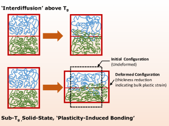
Figure 1: Comparison of polymer self-adhesion through diffusion at temperatures near or above T_g and the newly proposed sub-T_g, solid-state, plasticity-induced bonding in which bulk plastic deformation triggers the requisite molecular mobility for chain interpenetration across the interfaces.

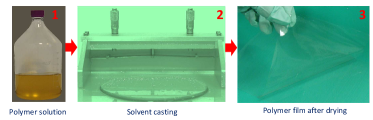
Figure 2: Steps involved in the preparation of polymer films through solvent casting: (1) a homogeneous solution of polymer and plasticizer in ethanol and water, (2) spreading of the solution on a glass surface via a knife, and (3) evaporation of solvents and formation of a glassy film after drying.

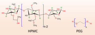
Figure 3: Molecular structures of hydroxypropyl methylcellulose (HPMC) and polyethylene glycol (PEG).

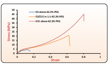
Figure 4: True stress-strain curves for three film formulations: E3-alone-42.3% PEG, E3/E15 in 1:1-42.3% PEG and E15-alone-42.3% PEG at ambient temperatures. The nominal strain rate for tensile testing was chosen as 0.0025 sec^-1.

Polymeric films were prepared by solvent casting (as shown in Figure  2) using a base polymer (hydroxypropyl methylcellulose) and a plasticizer (polyethylene glycol, PEG-400). The base polymer HPMC was available under the trade name METHOCEL in E3 and E15 grades. The molecular structures are shown in Figure  3. The films were assigned a name depending on the base polymer and weight percent (wt.%) of the plasticizer in the film with respect to the base polymer (see Methods and Supplementary Section 1). Films made from E3-alone-42.3% PEG, E3/E15 in 1:1-42.3% PEG and E15-alone-42.3% PEG exhibited T_g values in the range of 72–78^∘C. (See Methods and Supplementary Section 2.2). Their true stress-strain curves in tension are shown in Figure  4. All three films exhibited ductility, represented by their ability to undergo plastic flow.

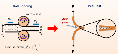
Figure 5: Roll-bonding was achieved by passing a stack of film layers with a total initial thickness t₁ between compression rollers to yield a final-thickness t₂. The peel-test was carried out on roll-bonded sample at the middle interface.

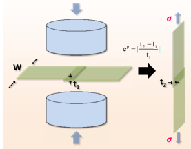
Figure 6: Lap specimens were prepared between two film layers by applying compression loads on the overlapping area. Lap shear-strength measurements were performed in a tensile mode.

Bonding experiments were carried out at ambient conditions. (i) Stacks of six film layers (each layer $\sim$100 $\mu$m) were fed through a roll-bonding machine to achieve active plastic deformation at ambient temperatures. Peel tests were performed to measure the mode I fracture toughness (G_c [J/m² ]), Figure  5, and (ii) lap specimens were prepared to measure the shear-strength ($\sigma_{s}$ [MPa]), Figure  6 (see Methods and Supplementary Section 4 for details on roll-bonding, peel testing and lap shear strength testing). G_c represents the work done per unit area for debonding the interface during a peel test. $\sigma_{s}$ indicates the maximum shear stress sustained by the bonded interface before failure. The effective thickness reduction was used as a measure of plastic strain during bonding in all of the cases.

Figure  7 shows a snapshot of several layers of the film (E3/E15 in 1:1-42.3% PEG) with an initial thickness of t₁=0.60 mm undergoing roll bonding through active plastic deformation with a final thickness reduced to t₂ =0.533 mm (see supplementary video S1).

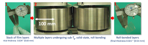
Figure 7: Illustration of sub-T_g, solid-state, plasticity-induced roll bonding of E3/E15 in 1:1-42.3% PEG films nearly 60 K below T_g. For this case, the nominal thickness strain is e_p= $|t_{2}-t_{1}|$/$t_{1}$=11.7%.

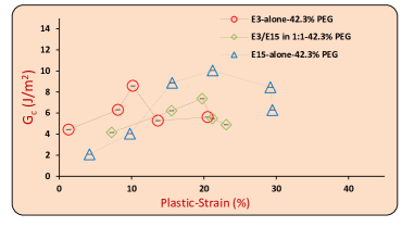
Figure 8: Fracture toughness (G_c [J/m²]) versus plastic strain plots for E3/E15 in 1:1-42.3%PEG, E3-alone-42.3%PEG and E15-alone-42.3%PEG.

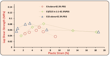
Figure 9: Lap shear-strength ($\sigma_{s}$ [MPa]) versus plastic strain plots for E3/E15 in 1:1-42.3%PEG, E3-alone-42.3%PEG and E15-alone-42.3%PEG.

The G_c results for the three films are shown in Figure  8. G_c correlated with the plastic strain in a non-monotonic fashion, first increasing and then decreasing. The adhesion between two interfaces held together by van der Waals forces, hydrogen bonds, or chemical bonds can only give G_c values in the range of 0.05 J/m² , 0.1 J/m² and 1.0 J/m², respectively [27]. The surface energy of glassy polymers itself is quite small [16] (on the order of 0.08 J/m²); therefore, negligible adhesion is noted when two such surfaces are brought into mere molecular proximity. However, glassy polymers can exhibit higher fracture toughness owing to the irreversible deformation of the macromolecules. The quantitative levels of G_c obtained here, with a maximum value nearly 10 J/m², could only be attributed to the irreversible processes of chain pull-outs, disentanglement and/or scissions during debonding, which could only happen if plasticity-induced molecular mobilization and chain-interpenetration led to bonding. Even polymer adhesion leading to G_c values as low as 1.2 J/m² [12] and 2.0 J/m² [71] has been attributed to irreversible chain pull-out mechanisms during fracture. Other mechanisms of adhesion such as acid-base interactions, capillary effects, electrostatic forces and/or any other conceivable mechanism do not apply in the current context (for a detailed discussion on the types of forces giving rise to adhesion, see [53]). The shear strength ($\sigma_{s}$) plots, shown in Figure  9, also exhibited a non-monotonic correlation with the bonding plastic strain. Quantitative levels of the $\sigma_{s}$ values reported here compare with those in [13], in which adhesion due to interdiffusion of chains below the bulk T_g over long times, on the order of several minutes, was reported. The reported levels of bulk plastic strains also rule out mechanical interlocking of asperities to cause adhesion because, at the levels of plastic strains reported here, the surface asperities would necessarily flatten out. Surface characterization of the films through AFM, before bonding, revealed nano-scale roughness (R_a) on the order of 6.91-22.7 nm (see Supplementary Section 2.6). By contrast, high levels of plastic strain led to an increased contact area, and if factors other than chain interpenetration were responsible for bonding, we would expect a monotonic increase in G_c or $\sigma_{s}$. The lowering of G_c or $\sigma_{s}$ at high levels of plastic strain could be explained on the basis of anisotropic growth in the microstructure such that the polymer chains oriented in the direction of the principal stretches (compression and rolling directions). We suggest that increasing levels of such chain orientation ultimately lead to less effective chain interpenetration across the interface, which diminishes bonding at higher strain.

A comparison of the surface morphology before bonding and after the fracture is shown in Figure  10. The debonded surfaces indicated events of chain scissions or pull-outs due to fracture, which were similar to those reported upon fracture of polymers welded through interdiffusion [72, 23, 14].

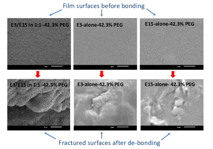
Figure 10: SEM images of E3/E15 in 1:1-42.3% PEG, E3-alone-42.3% PEG, and E15-alone-42.3% PEG, films before bonding and after debonding. The nominal plastic strains during roll-bonding for E3/E15 in 1:1-42.3% PEG, E3-alone-42.3% PEG, and E15-alone-42.3% PEG, films were 15.53%, 8.12%, and 10.18%, respectively.

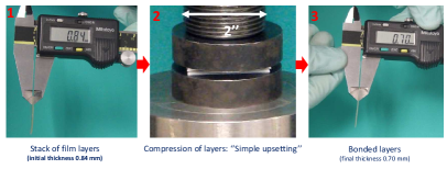
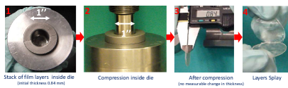
Figure 11: Compression of stacks of films (a) without any die containment to permit macroscopic plastic flow and bonding, (b) in a ‘hydrostatic die’ that is capable of generating high levels of hydrostatic pressure but limits the plastic flow, and consequently no bonding takes place. In both cases peak nominal compressive stresses (78.98 MPa) was kept same.

To explicitly demonstrate the role of bulk plastic deformation, we designed a ‘hydrostatic die’ setup, which was capable of generating high levels of hydrostatic pressure while inhibiting the macroscopic plastic flow. Figure  11 shows a comparison in which a stack of films (E3/E15 in 1:1-42.3% PEG) was compressed (i) without any constraints and (ii) with the ‘hydrostatic die’ constraint. In the first case, the stack underwent macroscopic plastic flow, and the layers bonded to form an integral structure, whereas in the case of the ‘hydrostatic die’ constraint, no permanent thickness change was observed, and the layers easily splayed apart after removal (see Supplementary video S2). In another experiment, we attempted to roll-bond E3/E15 in a 1:1-0% PEG film with E3/E15 in a 1:1-42.3% PEG film. Films with 0% PEG exhibited negligible plastic flow, and were therefore incapable of being subjected to plasticity-induced molecular mobilization, which also led to a no-bonding result (see Supplementary video S3). Nanoindentation experiments clearly revealed the differences between the elastic response of the 0% PEG films and the plasticity of the 42.3% PEG films (see Supplementary Figure 16). Both experiments demonstrated that activating bulk plastic flow on both sides of the interface was an essential requirement for bonding. This result also strongly reflected that effects such as the presence of a rubber-like layer at the surface, where the T_g may be lower than the bulk T_g and the time scales for segmental relaxations may be relatively small, by itself could not lead to adhesion of the magnitude observed during roll-contacts lasting on the order of a second (see supplementary Table 4 for estimates of the rolling times). Bonding below the bulk T_g (without any bulk plastic deformation), as reported in the literature, requires substantially longer durations. Furthermore, the existence of any enhanced relaxation of the polymer chains (or segments) in the surface layer would be severely restricted by any portions of the macromolecules extending into the glassy-bulk beneath; hence, long-range diffusion in a short time is not possible. Finally, although not considered in these prior reports, it is plausible that moderate contact pressures, applied over relatively long healing times at temperatures near T_g, contributed to mechanically enhanced molecular mobility that led to bonding via mechanisms similar to those described here.

Although rapid plastic deformation can cause a temperature increase, fully adiabatic analysis revealed an upper bound temperature increase of only 3.6^∘C (see Supplementary Section 3.3). The mechanically activated polymer mobility is mechanistically quite different from molecular mobility at temperatures above T_g. The shear transformation units of plastic deformation are also accompanied by local transient dilatations (volume changes) that can facilitate opportunities for establishing entanglements across the interface so that bonding can take place on the order of a second. The self-diffusion coefficient (D) of a polymer chain in its melt state shows a strong dependence on the molecular weight, D $\sim$ M ^-1 or D $\sim$ M^-2 in accordance with the Rouse or the reptation model, respectively. However, all three blends of polymer considered here, E3-alone, E15-alone and E3/E15 in 1:1, were roll-bonded on the order of a second, which was a significant contrast from the mechanism of polymer adhesion due to interdiffusion. The unprecedented aspects of the newly reported phenomenon and underlying mechanisms are expected to open new avenues for research and applications.

Methods

Film-Making:

Hydroxypropyl methyl cellulose (HPMC), trade name METHOCEL, in grades E3 and E15 was obtained from Dow Chemical (Midland, Michigan, North America). PEG-400 was purchased from Sigma-Aldrich (Milwaukee, Wisconsin, North America). Appropriate amounts of E3, E15 and PEG were mixed in desired amounts with ethanol and water, and a homogeneous solution was obtained through mixing with an electric stirrer for 24 h. After completion of the blending process, the solution was carefully stored in glass bottles at rest for 12 h to eliminate air bubbles. Solvent casting was carried out using a casting knife applicator from Elcometer (Rochester Hills, Michigan, North America) on heat-resistant borosilicate glass. All of the steps were carried out in a chemical laboratory where ambient conditions of 18^∘ $\pm$ 2^∘C and R.H. 20%$\pm$5% were noted. The residual moisture content in the films after drying was measured using Karl Fischer titration.

Bonding Experiments:

Roll bonding was carried out on a machine capable of exerting the desired load levels to achieve active plastic deformation. The 200 mm diameter rollers were operated at an angular speed of 0.5 rev/min, leading to an exit speed of 5.23 mm/s. Peel tests were carried out to measure mode I fracture toughness (see Supplementary video S4). Lap specimens were prepared using compression platens on an Instron mechanical tester. For both roll-bonded and lap specimens, for the sake of consistency, the adhesion measurements were carried out on the bonded interfaces between the top-top surfaces (exposed side during drying). Film layers were stacked accordingly. Top-bottom and bottom-bottom joining led to similar bonding results. The ‘hydrostatic die’ and ‘upsetting’ experiments were carried out on the Instron. The roll-bonding machine and fixture for the peel test were designed and fabricated in Massachusetts Institute of Technology (Cambridge, North America) (see Supplementary Section 4).

Characterization:

The molecular weights of E3 and E15 were estimated from viscosity measurements. The amorphous nature of the films were verified by XRD. SEM and AFM were performed to analyze the surfaces. DMA was performed to determine the T_g. Tensile stress-strain curve tests, fracture toughness through peel tests, and lap shear tests were carried out. Nanoindentation was carried out to measure the hardness. The specific heat capacity was measured using DSC.

The X-ray diffraction patterns were recorded using a PANalytical X’Pert PRO Theta/Theta powder X-ray diffraction system with a Cu tube and an X’Celerator high-speed detector. AFM images were obtained using a Dimension 3100 XY closed loop scanner (Nanoscope IV, VEECO) equipped with NanoMan software. Height and phase images were obtained in tapping mode in ambient air with silicon tips (VEECO). DMA was carried out on a TA Q800 instrument. Mechanical testing was performed on an Instron mechanical tester. Nanoindentation tests were carried out on a Triboindenter Hysitron instrument. Calorimetry was performed on a TA Q200 instrument. The viscosity was measured on an HR-3 Hybrid rheometer.

Acknowledgements:

The authors acknowledge the funding from Novartis Pharma AG and facilities at the Novartis-MIT Center for Continuous Manufacturing program [65] where this research was carried out. N.P. also appreciates discussions with Professor Robert E. Cohen.

Author Contributions:

N.P. conducted experiments, designed and developed the experimental set-ups, and wrote the letter and supplementary. D.M.P. identified the sub-T_g, solid-state, plasticity-induced bonding and provided supervision on the subject of mechanics. B.L.T. advised on the phenomenological aspects of adhesion and supervised the overall development of thin-film technology at MIT. A.H.S. supervised the design and development of mechanical fixtures and machines. D.M.P., B.L.T. and A.H.S jointly supervised the work. All authors contributed to review of the manuscript, and participated in discussions during this research.

1 SUPPLEMENTARY FILM-MAKING

Table 1: Formulations employed in making polymer films from HPMC E3 and E15 with different levels of plasticizer (the amounts have been rounded off to nearest grams).

Polymer film	Composition
	E3	E15	Water	EtOH	PEG
	(g)	(g)	(g)	(g)	(g)
E3/E15 in 1:1-0% PEG	15	15	96	96	0
E3/E15 in 1:1-28.5% PEG	15	15	96	96	12
E3/E15 in 1:1-42.3% PEG	15	15	96	96	22
E3/E15 in 1:1-59.5% PEG	15	15	96	96	44
E3-alone-42.3% PEG	30	0	96	96	22
E15-alone-42.3% PEG	0	30	96	96	22

Polymeric films employed in this study comprise of a base polymer hydroxypropyl methyl cellulose (HPMC) and a compatible plasticizer, PEG-400. HPMC is cellulose ether and available from Dow Chemical under the trade name of METHOCEL. We acquired METHOCEL E3 and METHOCEL E15 products from Dow Chemical.

HPMC is an uncrosslinked polymer and shows an excellent film formability due to its underlying cellulose structure in which all the functional groups lie in the equatorial positions, causing the molecular chain of cellulose to extend in a more-or-less straight line and easing the formation of the film. Table  1 shows the sample weights of the contents used in preparation of the solutions. Films were made through casting and drying of the prepared solutions. As seen in Table  1, films are referred to based on the amounts of E3, E15 and Wt.% of PEG-400. For example, E3/E15 in 1:1-42.3% PEG implies that E3 and E15 are present in one-to-one ratio and the Wt.% of PEG in the film is 42.3%, since 22 g PEG in 15 g E3 plus 15 g E15 is 42.3%.

Table 2: Residual moisture in films after drying, measured through Karl Fischer titration. %Wt. indicates residual moisture in the films after drying.

Polymer film	Residual H2O
	(%Wt.)
E3/E15 in 1:1-0% PEG	3.70
E3/E15 in 1:1-28.5% PEG	7.21
E3/E15 in 1:1-42.3% PEG	4.29
E3/E15 in 1:1-59.5% PEG	2.45
E3-alone-42.3% PEG	2.92
E15-alone-42.3% PEG	4.54

Karl Fischer titration was carried out to determine the residual moisture content in the films after drying. Dimethyl sulfoxide (DMSO) was used as a reagent for dissolving films. DMSO was purchased from Sigma Aldrich (ACS reagent grade). The solution of the dissolved film in DMSO was fed into the Karl Fischer Titrator, and the residual moisture was estimated. Table  2 shows the average amounts (repeated three times) of the estimated residual moisture contents in the films.

2 SUPPLEMENTARY CHARACTERIZATION

2.1 Role of Plasticizer and Mechanical Properties

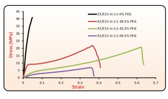
Figure 12: (a) Schematic role of plasticizer on molecular configurations, (b) Effect of PEG-400 on tensile true stress-strain behavior of polymeric films. The tensile tests were carried out at ambient temperature and a nominal strain rate of 0.0025 s^-1.

PEG-400 acts as a compatible plasticizer for HPMC. Inclusion of a plasticizer within the polymer matrix enhances its ductility (or plastic flow characteristics). Plasticizers work by embedding themselves between the chains of polymers and spacing them apart by increasing the free volume. By dissolving and mixing intimately, PEG molecules disrupt the secondary bonds between the polymer chains. Figure  12 illustrates this effect.

Figure  12 shows true stress-strain behavior of films made from E3/E15 in 1:1 with varying the PEG concentrations 0%, 28.5%, 42.3% and 59.5%, respectively. The plasticization effect of increasing PEG (Wt.%) is evidenced by the lowering of the initial modulus and the yield strength and, increase in the failure strain. The maximum failure strain occurs for 42.3% PEG film. Clearly, all films containing PEG demonstrate large ductility that is absent in 0% PEG film. The effect of including PEG on the lowering of glass transition temperature is discussed next.

2.2 Dynamic Mechanical Analysis

Dynamic Mechanical Analysis was performed on all the films listed in Table  1. A temperature sweep was performed at 1 Hz frequency. Figures  13(a) to  13(f), show the plots of loss modulus, storage modulus and tan $\delta$ for six different films. The glass transition temperature is determined by the peak in the tan $\delta$. For E3-alone-42.3% PEG T_g was estimated to be 72^∘ C, and for E15-alone-42.3% PEG and E3/E15 in 1:1-42.3% PEG T_g was estimated as 78^∘ C. Inclusion of PEG evidently lowers the glass transition temperature and broadens the temperature range over which the glass transition takes place.

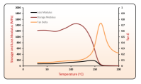
(a) E3/E15 in 1:1-0% PEG

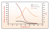
(b) E3/E15 in 1:1-28.5% PEG

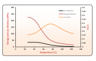
(c) E3/E15 in 1:1-42.3% PEG

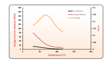
(d) E3/E15 in 1:1-58.5% PEG

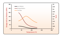
(e) E3-alone-42.3% PEG

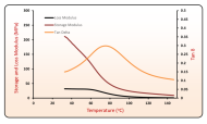
(f) E15-alone-42.3% PEG

Figure 13: Dynamic Mechanical Analysis Curves.

2.3 Molecular Weight

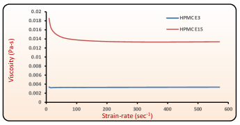
Figure 14: Viscosity curves of 2% aqueous solution of METHOCEL-E3 and METHOCEL-E15.

Viscosity measurements for 2% aqueous solution of E3 and E15 were carried out based on the procedure prescribed by Dow [3]. The viscosity curves for E3 and E15 are shown in the Figure  14. E3 solution shows negligible rate dependence; with the viscosity lying in the range 3 – 4 mPa-s. E15 solution shows some rate dependence with viscosity lying in the range 14 – 21 mPa-s. From the Dow Chemical manual [2], the viscosity for 2% aqueous solution of different grades E3, E5, E6, E15 and E50 are specified as 3, 5, 6, 15 and 50 mPa-s, respectively. In another Dow manual [1], the ranges for the viscosity of 2% Wt. solution of E3 and E15 are specified as 2.4 – 3.6 mPa-s and 12 – 18 mPa-s, respectively. Our measurements overlap well within these specifications. If we choose a representative viscosity of 3.8 mPa-s for E3 and 16 mPa-s for E15, then based on the viscosity and molecular weight relationship from [2], we estimate the number average molecular weight (M_n) for E3 and E15 approximately as 8,200 and 20,000, respectively.

A detailed molecular characterization of METHOCEL cellulose ethers presented in [44], also led to estimation of weight average (M_w) and number average (M_n) molecular weights as: (i) E3: M${}_{n}=8,100$ and M${}_{w}=20,300$ with M_w/M_n = 2.5, and (ii) E15: M${}_{n}=24,800$ and M${}_{w}=60,300$ with M_w/M_n = 2.4. Such estimations are consistent with those we obtained. In the same study [44], the degree of polymerization (DP) was reported as: (i) E3, DP= 77, and (ii) E15, DP=296, and the weight average radius of gyration (R_gw) as: (i) E3, R_gw = 7.4 nm, and (ii) E15, R_gw = 15.1 nm.

2.4 X-Ray Diffraction

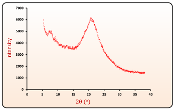
Figure 15: XRD of E3/E15 in 1:1-42.3% PEG.

HPMC is a cellulose derivative and well known to exist in amorphous form. To verify the amorphous characteristic, an X-ray diffraction was carried out on E3/E15 in 1:1-42.3% PEG, shown in Figure  15. As expected, a diffused pattern without any peaks is obtained, thus, indicating absence of any crystallinity.

2.5 Nanoindentation

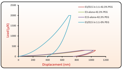
Figure 16: Nanoidentation load versus displacement curves for E3/E15 in 1:1-0% PEG, E3/E15 in 1:1-42.3% PEG, E3-alone-42.3% PEG and E15-alone-42.3% PEG films. Indentation experiments were carried out in load controlled mode with chosen peak loads up to 300 $\mu$N and 2000 $\mu$N for films with 42.3% PEG and 0% PEG, respectively.

Nanoindentation experiments were performed on E3/E15 in 1:1-0% PEG, E3/E15 in 1:1-42.3% PEG, E3-alone-42.3% PEG and E15-alone-42.3% PEG films. The experiments were carried out in a force controlled mode with a maximum force of 2000 $\mu$N and 300 $\mu$N for 0% PEG and 42.3% PEG films, respectively. A larger load for the 0% PEG film was chosen in order to activate sufficient plastic indentation so that its hardness could be measured. Berkovich indenter with a root radius of 150 nm was used. The load versus displacement curves for all the films are shown in the Figure  16. The film with 0% PEG shows a relatively large indentation force and large elastic recovery, whereas films with 42.3% PEG films show little elastic recovery and large residual indentation depth. Based on these behaviors, the 0% PEG film can be called an ‘elastic’ film and the 42.3% PEG film as a ‘plastic’ film.

Using Oliver-Pharr method we estimated the hardness from the nano-indentation tests. The hardness values for E3/E15 in 1:1-0% PEG, E3/E15 in 1:1-42.3% PEG, E3-alone-42.3% PEG and E15-alone-42.3% PEG films were 144.0 MPa, 10.83 MPa, 10.151 MPa, and 11.48 MPa, respectively. This shows that the film with 0% PEG is “hard” and unlikely to demonstrate plasticity-induced molecular mobilization for bonding at the load levels where 42.3% PEG films exhibit sufficient plastic flow. This is also consistent with the no-bonding outcome between 0% PEG film and 42.3% PEG film, as shown in the Supplementary video S3.

2.6 Atomic Force Microscopy

Figure  17 shows sample AFM scans of a 5 $\mu$m x 5 $\mu$m area on the top surface of three films with 42.3% PEG, along with the average roughness given by $R_{a}=\frac{\sum_{1}^{n}|y_{i}|}{n}$. The top surfaces of films exhibit nano-scale roughness, however, this scale of roughness does not play any important role when we have reported bulk plastic strains essential for bonding.

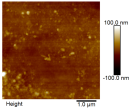
(a) Top surface of E3/E15 in 1:1-42.3% PEG film, $R_{a}=$ 6.91 nm

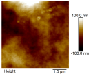
(b) Top surface of E3-alone-42.3% PEG film, $R_{a}=$ 22.7 nm

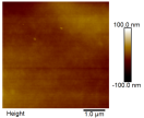
(c) Top surface of E15-alone-42.3% PEG film, $R_{a}=$ 8.63 nm

Figure 17: Measurement of Nanoroughness using Atomic Force Microscopy.

3 SUPPLEMENTARY DISCUSSION

3.1 Polymer Dynamics and Self-Diffusion

Polymer melts are an equilibrium system and their mobility is commonly described by the models of Rouse, reptation, etc. The fundamental dynamic property that characterizes the average motion of a polymer chain is the coefficient of self-diffusion (D). In the Rouse regime, polymer chains are unentangled and the diffusion coefficient D_rouse $\sim$N^-1, where N is number of monomers. In the reptation regime polymer chains experience topological constraints, and the lateral displacements in the entangled chain structure are negligible compared with the longitudinal diffusion or “reptation” in the “tube” formed by neighboring molecules with D_reptation $\sim$N^-3. The transition from Rouse to reptation regime is often noted at the critical entanglement length N_e. The self-diffusion coefficient in polymer melts strongly depends on the temperature, molecular weight, and molecular characteristics. Typical values of self-diffusion coefficient are listed in Table  3.

Table 3: A Short Summary of Self-Diffusion Coefficient (D) from literature. T_m and T_g stand for melting and glass transition temperature, respectively.

Ref.	Polymer	Mol. Wt.	Temp.	D	Comments
		(g/mol)	(K)	(m2/s)
[11]	Linear H-PB	5$\times$104 – 20 $\times$ 104	398.15	10-14 – 5$\times$10-16	Tm $\sim$ 381.15 K
[34, 29]	Polyisoprene	560 – 9.82$\times$ 104	373.15	2.2$\times$10-10 – 1.0$\times$10-14	Tg $\sim$ 192 K [4]
[34]	Polybutadiene	690 – 4.99$\times$104	373.15	7.0$\times$10-11 – 2.0$\times$10-14	Tg $\leq$ 183.15 K
[61]	Polyethylene	200 – 12$\times$104	448.15	6.6$\times$10-10 – 1.3$\times$10-14	Tm$\sim$ 353.15 – 400.15 K
[46]	PDMS	500 – 5$\times$105	293.65	7.0$\times$10-10 – 5$\times$ 10-15	Tg $\sim$ 150.15 K
[33]	PS	600 – 19$\times$103	487.8	2.5$\times$10-10 – 1.5$\times$ 10-13	Tg $\sim$ 333.15 – 373.15 K

Usually, the diffusivities of the polymer melts are quite small compared to the liquids composed of simple molecules (for example D_water at 298.1 K and 1 atm is nearly 2.3$\times$10^-9 m²/s [49]). However, high diffusion coefficients for polymer melts can be noted when molecular weights are small and temperatures are well above the melting point or the glass transition temperature.

When the temperature of a glass forming liquid is lowered and the glass transition temperature is approached from the above, kinetics of a glass-forming system shows a drastic slow down, and time scales for relaxations become orders of magnitude larger than at higher temperatures representative of the melt. As an example, in [69] the self-diffusivity of a single component glass former, tris- naphthylbenzene (TNB), falls from D $=$ $10^{-14}$ m²/s at 405 K to D = $10^{-20}$ as T_g (close to 335 K) is approached. In [56] it was shown that as T_g is approached from above the diffusivity for o -terphenyl (OTP) is of the order $10^{-20}$ m²/sec. Similar slow downs of self-diffusion, with D approaching 10^-20 m²/s near the glass transition temperature, were noted for o-terphenyl and metallic melts of Pd–Cu–Ni–P systems [63].

The Bueche-Cashin-Debye equation [19, 18], which relates diffusivity and viscosity, is given as:

$$\frac{D\eta}{\rho}=\frac{AK_{B}T}{36}\frac{R^{2}}{M}$$ (1)

In the above equation, A is the Avogadro constant, K_B is the Boltzmann constant, T is the absolute temperature, R² is the mean-square end-to-end distance of a single polymer chain, and M is the molecular weight. If we estimate D for our polymer at the glass-transition temperature by considering $\eta$=10¹³ Poise, $\rho$=1180 Kg/m³, R²= 6$\times$7.4² nm² (using R_g of E3, and R²=6$\times$ R${}_{g}^{2}$) and M=20,300 g/mol, T = 352 K, the estimated value of D is 1.12$\times$ 10^-24 m²/s. This is a remarkable estimate in terms of the order of magnitude and compares well with the self-diffusivity of 10^-25 m²/s as reported in [52]. Such small diffusivity near T_g clearly indicates the aspect of kinetic arrest as the glass transition temperature is approached.

If we consider a scenario: in which a diffusion distance of x=10 nm is to be achieved in a time of one second, then D must be greater than 0.5$\times$10^-16 m²/s. This is impossible in the solid-state, 60 K below the bulk-T_g, and clarifies the distinction of polymer welding above T_g with respect to newly reported plasticity-induced molecular mobilization and bonding which occurs in a period of time on the order of a second.

3.2 Stress-Induced Molecular Mobility and Plastic-Deformation

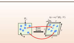
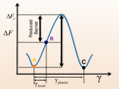
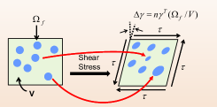
Figure 18: Mechanism of plastic deformation and shear transformation in glassy polymers [8]. (a) A unit shear transformation in a kinetically trapped state under shear stress comprises of an initial elastic shear-strain which is followed by plastic-relaxation of polymer chain segments. (b) Free energy landscape, associated with a polymer chain, during a unit shear transformation (c) Accumulation of several shear transformations leads to macroscopic plastic deformation.

In 1936, Eyring undertook an absolute reaction-rate approach to demonstrate the effect of stress on lowering of viscosity in certain gels, glasses or crystals and enhancement of molecular mobility. According to Erying’s model:

$$\frac{1}{\nu_{1}}={\tau_{\alpha}(T,\tau)}=\tau_{o}\cdot exp\left[\frac{E_{A}-\tau V^{*}}{K_{B}T}\right]$$

Here, $\nu_{1}$ is the jump frequency (inverse of the relaxation time) of the molecules in the direction of applied stress, $\tau_{o}$ is a constant (vibration time scale), $\tau$ is the applied shear stress, $V^{*}$ is the activated volume, $E_{A}$ is the potential barrier that molecules have to overcome in going from one configuration to another. The above equation states that the relaxation time decreases in the direction of the applied shear-stresses and molecular transport is facilitated in the direction of shear stresses. However, Eyring’s model is found to be applicable only in the regimes of linear visco-elasticity for polymers, and fails to capture the dramatic changes in the energy landscapes associated with plastic deformation of a glass.

As stated in the main letter, plastic deformation in polymers at a continuum scale is understood in terms of shear transformations i.e. events of spatial rearrangements of molecular clusters causing stress-relaxation. Consider the scenario shown in the Figure  18: well below T_g, the polymer chains are kinetically trapped in their local configurations and timescales for mobility (specifically translation motions) of these chains are extremely large. However, application of shear-stress on the material element causes its deformation and the polymer chain under consideration changes its orientation: first elastically, and then due to some local perturbation it relaxes plastically while overcoming the potential barrier set up due to neighboring molecules.

If no stresses were applied and temperature were held far below T_g then the transition of the mean configuration of a polymer chain from its kinetically trapped configuration would not happen on experimental time scales. However, qualitatively speaking, the application of stress enhances the mobility of the polymer chain as it relaxes, and changes its configuration on experimental time scales. Effect of such cumulative events during active plastic deformation characterize the enhanced dynamics in deforming glasses below T_g.

We emphasize that by kinetically trapped state of a glass it is implied that any cooperative segmental relaxations or long range diffusive motions of chains are severely restricted; however, secondary relaxation processes (those corresponding to vibrations of side groups like $\beta$, $\gamma$, $\delta$, etc. relaxations) may still be active. But, such weak secondary relaxation processes are incapable of giving any interdiffusion and pronounced adhesion in a short-time when two interfaces are brought together in molecular proximity, unless enhanced mobility is triggered through plastic deformation.

The fundamental differences between polymer mobility at high temperatures (well above T_g) and stress-assisted molecular mobility (well below T_g) can be summarized as follows: The motion of polymer chains (or segments) in a polymer melt can be described based on diffusion models. It primarily occurs due to high kinetic energy of the polymer chains (or segments), and available free-volume (or physical space) due to which chains (or segments) can sample new orientations effectively. The polymer melts (above T_g) are spatially homogeneous and thermodynamically in an equilibrium state, whereas, plastic deformation and associated enhanced mobility in a glassy polymer is not at all an equilibrium concept. The root mean square displacement of center of mass of a polymer chain will increase monotonically with time during diffusion in a polymer melt, however, the mechanically assisted enhanced mobility in polymers only occurs during active plastic deformation and stops when plastic straining stops. The average kinetic energy of a polymer molecule is large in a polymer melt compared to that in the solid-state glass well below T_g. Typical values of activation energy for diffusion in molecular liquids at room temperature can be as low as 5-10 kcal/mol and therefore diffusion can be thermally activated. However, for a shear-transformation the activation energy (for example inorganic glasses is 350-400 kcal/mol [8]) and therefore plastic deformation is not thermally activated at room temperatures on experimental time scales. Although plastic deformation can be accompanied by a temperature rise, at relatively slow strain-rates the associated temperature rise is negligible.

3.3 Temperature Rise

It is worth checking for any temperature rise due to irreversible mechanical work during plastic deformation, and if such temperature rise is responsible for enhanced molecular mobility leading to bonding. As an illustration, we measured the specific heat of E3/E15 in 1:1-42.3%PEG film through differential scanning calorimetry, as shown in Figure  19. From the rate of heat flow into the sample and specified rate of temperature rise during thermal scan the C_p is obtained as $1860$ J/Kg-K, and the density was measured to be $\rho=$ $1180$ Kg/m³. Based on the stress-strain curves if we estimate the flow stress for plastic deformation to be $\sigma_{f}=8$ MPa, then for a plastic strain of $\epsilon_{p}=$ $0.5$, the adiabatic temperature rise is estimated to be:

$$\triangle T=\frac{\sigma_{f}\epsilon_{p}}{\rho C_{p}}=3.6^{\circ}C$$

As seen here, the temperature rise according to fully adiabatic analysis is quite small. External work due to the application of stresses leads to mechanically-assisted (and not temperature assisted) enhanced mobility of polymer chains (or segments). The operative micro-mechanisms of plastic-relaxation at a molecular level are dependent on particular molecular characteristics, and may at best be explored through computer simulations. In our opinion, this remains as an open question.

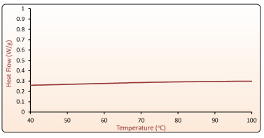
Figure 19: DSC scan of E3/E15 in 1:1-42.3% PEG film.

4 Bonding Experiments

4.1 Roll-Bonding Machine

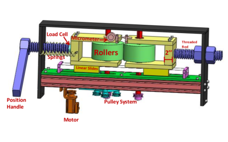
Figure 20: A roll-bonding machine to carry out sub-T_g, solid-state, plasticity-induced bonding.

Figure  20 shows a CAD model of the roll-bonding machine designed for this work. The machine is capable of achieving different levels of plastic strain by adjustment of the gap between the rollers and monitoring the compression load during rolling. The angular speed of the rollers is controlled using a stepper motor. The radius of the rollers (R) is 100 mm, much larger than the total initial thickness of a film-stack (t₁), which is typically less than 1 mm. The incoming stack of film behaves like a thin strip and through-thickness plastic deformation is triggered under such conditions. From kinematics of rigid-plastic rolling of thin-strip [38] the time spent during active plastic deformation can be estimated as follows:

$$\tau=\frac{\sqrt{R(t_{1}-t_{2})}}{V_{2}}$$ (2)

In the above equation, t₁ is the initial thickness of film-stack, t₂ is the thickness of film-stack at the exit, V₂ is the linear speed at the exit. For V₂ = 5.23 mm/s, t₁=.6 mm and t₂=0.45 mm (indicating 25% nominal plastic strain), the time spent by a material element under the roller would be approximately 0.74 s. This is how we achieve sub-T_g, solid-state, plasticity-induced roll-bonding in a period of time on the order of a second. The Supplementary video S1 demonstrates how a stack of films with a certain initial thickness is subjected to active plastic straining leading to sub-T_g, solid-state, plasticity-induced bonding. The final thickness of the roll-bonded stack is less than the initial. Complete details on the roll-bonding machine and process will be available in [59].

Table 4: For a given exit speed (V₂ = 5.23 mm/sec) and an initial thickness t₁ = 0.6 mm, estimates of time spent under the roller bite during plastic straining.

Plastic Strain	t2	Time
	(mm)	(seconds)
0.05	0.57	0.33
0.1	0.54	0.47
0.15	0.51	0.57
0.20	0.48	0.66
0.25	0.45	0.74

4.2 Mechanics of Peel Test

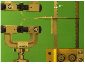
Figure 21: Peel-Test in mechanical tester to determine mode-I fracture toughness (G_c).

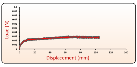
Figure 22: Force versus displacement curve during Peel-Test. In the steady-state peeling the peel-force becomes steady with respect to cross-head displacement.

Figure  21 shows a snapshot of the peel test. A peel test fixture was designed to perform accurate mode-I fracture. Such a test is also commonly known as T-peel test in the literature. The designed fixture [60], provides support to a long tail of the peel-specimen and eliminates any spurious effects due to gravity. When a stack of six layers is roll-bonded then a total of five bonded interfaces are formed. Peeling is done at the central interface. Figure  22 shows force versus displacement curve during the peel test. For all peel tests a cross-head speed of 15 mm/min was chosen. The steady-state peeling force $P$ is used to estimate the rate of external work per unit advance of crack as 2P/b, where ‘b’ is the width of the specimen (typically 15 – 20 mm). In order to correctly determine the fracture toughness (G_c) of the plastically-welded interface, any amount of plastic work due to bending of peel arms must be subtracted from the total steady state work [45]. Next, we present the mechanics of the peel test and methodology to estimate the correct interface toughness (G_c). The correction factor is adopted from [45]. The error bars in $G_{c}$ (as shown in the main letter) are based on the variation when peeling force becomes steady.

Elastica Analysis

If the bending of the peel arm leads to only small elastic strains with possibly large rotations then it is referred to as an elastica. Figure  23 schematically shows a peel test, where symbols have following meaning:

P is the vertical force applied by the upper-grip at ‘A’ [N]
M_f is the moment applied by the upper-grip at ‘A’ on the peel-arm ‘OA’[N$\cdot$m]
M_b is the moment exerted at ‘O’ on the peel-arm ‘OA’ [N$\cdot$m]
t is the thickness of the peel-arm [m]
$\theta$ is the angle made by the tangent at any point along the peel-arm with respect to horizontal [rad]
$\sigma_{y,t}$ is the yield-strength of the material in tension [MPa]
$\sigma_{y,c}$ is the yield-strength of the material in compression [MPa]
$\nu$ is the Poisson’s ratio
E is the elastic modulus [Pa]
E’=$\frac{E}{1-\nu^{2}}$ is the plane-strain elastic modulus [Pa]
t is the thickness of one peel-arm [m]
b is the width of the peel-arm into the plane [m]
s is the coordinate along the peel-arm [m]
I$=\frac{bt^{3}}{12}$ is the moment of inertia of beam out of plane [m⁴]
$\rho=\frac{ds}{d\theta}$ is radius of curvature at any point on the beam [m]
$\kappa=\frac{1}{\rho}$ is the curvature [m^-1]
U is the elastic energy due to bending [J]
G_c is the critical energy release-rate [J$\cdot$m^-2]
k$=\frac{P}{E^{\prime}I}$ is a constant defined for convenience [m^-2]

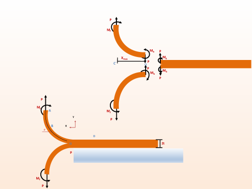
Figure 23: Schematic of an elastica. For the sake of clarity only the forces and moment on the upper-peel arm at the crack tip due to lower arm are indicated as M_b and P.

In Figure  23, the crack tip location is marked at the location ‘O’. The upper peel-arm is shown as ‘O-A’ along with the forces acting on it. During the peel test, both the peel-arms are clamped in the tensile-tester. We shall carry out the analysis on the upper peel-arm (and symmetrical conditions hold for the lower peel-arm).

When the width ‘b’ of the peel-specimen is considerably larger than the thickness; then plane-strain conditions prevail. In our case ‘b’ is 15 – 20 mm and ‘t’ is 0.2 – 0.4 mm, hence plane strain bending scenario is assumed. In this plane strain problem $\epsilon_{z}$ is zero, and only $\sigma_{x}$ and $\sigma_{z}$ are non-zero stress components. Adapting elementary beam theory to plane strain, we have:

$$\sigma_{x}=E^{\prime}\epsilon_{x}$$ (3)

where, $\epsilon_{x}=-\frac{y}{\rho}$ (y=0 is the middle thickness of the top elastica ‘OA’). The elastica is assumed to be inextensible, implying no stretching of the neutral axis under tension. The moment (M) at any section relates to the radius of curvature as:

$$M=\frac{E^{\prime}I}{\rho}.$$ (4)

Equilibrium of an element along the beam at point ‘B’, with coordinates (x,y) and angle $\theta$, leads to

$$E^{\prime}I\frac{d\theta}{ds}=P(x_{max}-x)+M_{f};$$ (5)

differentiating the equation  5 with respect to ‘s’, give

$$E^{\prime}I\frac{d^{2}\theta}{ds^{2}}=-P\frac{dx}{ds}.$$ (6)

From the coordinate rule we know that,

$$ds\;cos(\theta)=dx$$ (7)

and

$$ds\;sin(\theta)=dy.$$ (8)

Substituting equation  7 in equation  6,

$$E^{\prime}I\frac{d^{2}\theta}{ds^{2}}=-Pcos(\theta),$$ (9)

and on re-arranging,

$$\frac{d^{2}\theta}{ds^{2}}+kcos(\theta)=0$$ (10)

where, $k=\frac{P}{E^{\prime}I}$.

Now use a substitution $\frac{d\theta}{ds}=v$, and integrate the above equation to get

$$\frac{v^{2}}{2}+ksin(\theta)=c_{1}$$ (11)

where $c_{1}$ is the constant of integration, and it can be obtained through boundary conditions on $v$ ($\frac{d\theta}{ds}$).

Using equations  7,  8 and  11, we can find:

$$S=\int_{0}^{s}ds=\int_{0}^{\theta}\frac{d\theta}{\sqrt{2(c_{1}-ksin(\theta))}}$$ (12)

$$X=\int_{0}^{x}dx=\int_{0}^{\theta}\frac{cos(\theta)d\theta}{\sqrt{2(c_{1}-ksin(\theta))}}$$ (13)

$$Y=\int_{0}^{y}dy=\int_{0}^{\theta}\frac{sin(\theta)d\theta}{\sqrt{2(c_{1}-ksin(\theta))}}$$ (14)

The above expressions also have an analytic solution in a specific case (as given in [45]). It is important to note that Y and S can grow unbounded (depending upon the boundary conditions).

We are interested in the conditions for:

(i) Elastica, and

(ii) Long peel-arm during steady-state

The boundary conditions, in Figure  23, can be set as $M_{f}=0$ at $\theta=\pi/2$, or curvature $\frac{d\theta}{ds}=\kappa_{b}=0$ at $\theta=\pi/2$.

Now using equation  11 we get

$$c_{1}=k=\frac{P}{E^{\prime}I}$$

Thus, integrals  12,  13,  14 can be reduced to

$$S_{total}=\int_{0}^{s}ds=\int_{0}^{\pi/2}\frac{d\theta}{\sqrt{2k(1-sin(\theta))}}$$ (15)

$$X_{max}=\int_{0}^{x}dx=\int_{0}^{\pi/2}\frac{cos(\theta)d\theta}{\sqrt{2k(1-sin(\theta))}}$$ (16)

$$Y_{max}=\int_{0}^{y}dy=\int_{0}^{\pi/2}\frac{sin(\theta)d\theta}{\sqrt{2k(1-sin(\theta))}}$$ (17)

It is important to note that equations  15 and  17 represent improper integrals of second kind since the function to be integrated is unbounded in the specified limits.

This implies that elastica becomes vertical only asymptotically in the absence of any moment at the upper-grip. Numerical integration method can be employed by carrying out the integration in the range [0, $\pi/2$).

Next, we are interested in calculating the net energy stored in the (part-of) elastica, from $0$ to $\theta$, and this integral turns out to be a proper integral.

For an element under bending as shown in Figure  24, we have

$$M=\frac{E^{\prime}I}{\rho}=\kappa E^{\prime}I$$ (18)

and

$$\alpha=\kappa ds$$ (19)

Thus, differential-energy stored in an element $ds$ in bending from $0$ up to an angle $\alpha$ (or curvature $\kappa$) is

$$U_{element}(\alpha)=\int dU_{element}=\int_{0}^{\alpha}M(\alpha)d\alpha$$ (20)

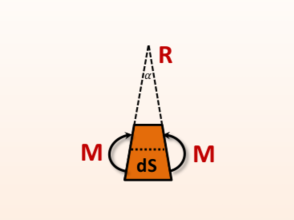
Figure 24: Energy in bending.

Using equations  18 and  19 we can also write

$$dU_{element}(\kappa)=E^{\prime}I\kappa\;d\kappa\;ds$$ (21)

Thus,

$$U_{element}(\kappa)=\int_{0}^{\kappa}E^{\prime}I\kappa\;d\kappa\;ds=E^{\prime}I\frac{\kappa^{2}}{2}ds$$ (22)

Thus, the energy of the (part-of) elastica from ‘O’ up to any point along on it is given as

$$U_{net}(s)=\int_{0}^{s}E^{\prime}I\frac{\kappa^{2}(s)}{2}ds$$ (23)

If converted in terms of $\theta$ we get

$$U_{net}(\theta)=\frac{E^{\prime}I}{2}\int_{0}^{\theta_{f}}\sqrt{2k(1-sin(\theta))}\;\;d\theta$$ (24)

For $\theta_{f}=\pi/2$, U_net is the total energy of the elastica. The total bending energy is always finite even though the length of the elastica is unbounded, and it is worth emphasizing that this is correct when the elastica is assumed to be inextensible. We shall see some illustration graphs shortly. But, first we shall establish the conditions in which the limit of elastica is broken and plasticity starts due to bending.

Conditions for Onset of plasticity

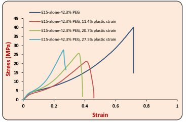
Figure 25: True stress-strain curves under tension for E15-alone-42.3% PEG, after roll-bonded at different levels of nominal plastic strain.

If we assume isotropic material behavior, with $\sigma_{y,c}=\sigma_{y,t}$, the location of maximum curvature $\kappa$ occurs at ‘O’. Although glassy polymers may exhibit both kinematic and isotropic hardening, films with 42.3% PEG exhibited negligible changes in tensile yield stress even for plastic strain up to 25%; and therefore the original properties of films (before rolling) were chosen for analysis below. As an illustration, Figure  25 shows the true stress-strain curves in tension for E15-alone-42.3% PEG films roll-bonded at different levels of nominal plastic strain. It is seen that yield points of films in tension after roll-bonding at different levels of plastic strain are not much different than the yield point of the starting film. This indicates that effect of plastic strain during roll-bonding on the yield strengths of the films is negligible.

The plane-strain condition and von-Mises yielding conditions imply that onset of yielding is marked by:

$$\sigma_{x}=\frac{\sigma_{yield}}{\sqrt{1-\nu+\nu^{2}}}$$ (25)

The maximum bending stress occurs at the base and is given as:

$$\sigma_{max}=\frac{M_{b}t/2}{bt^{3}/12}=\frac{6M_{b}}{bt^{2}},$$ (26)

Thus, setting $\sigma_{max}=\frac{\sigma_{yield}}{\sqrt{1-\nu+\nu^{2}}}$ we get the maximum bending moment at the base as:

$$M_{b,max}=\frac{\sigma_{yield}bt^{2}}{6\sqrt{1-\nu+\nu^{2}}}$$ (27)

Since, $M_{b}=\kappa E^{\prime}I$ i.e.

$$\kappa_{b,max}=\frac{\sigma_{yield}bt^{2}}{6E^{\prime}I\sqrt{1-\nu+\nu^{2}}}$$ (28)

Now using equation  11,

$$\frac{\kappa_{b,max}^{2}}{2}=\frac{P_{max}}{E^{\prime}I}$$ (29)

This leads to:

$$P_{max}=\frac{\sigma_{yield}^{2}bt}{6E^{\prime}(1-\nu+\nu^{2})}$$ (30)

If we stay within the limits of the onset of plasticity then elastica analysis applies. If the peel-arm is long enough then the steady-state bending energy of the elastica is constant (given by equation  24), and all the external work goes into the debonding process, and fracture toughness is given as:

$$G_{c}=\frac{2P}{b}$$ (31)

The maximum G_c before the onset of plasticity is given as:

$$G_{c,max}=\frac{2\sigma_{yield}^{2}t}{6E^{\prime}(1-\nu+\nu^{2})}$$ (32)

Whenever experimentally measured steady-state peel force is greater than P_max (estimated by equation  30), a correction based on [45] is applied. In steady-state the plastic work due to bending is subtracted from the total work and corrected interface toughness is estimated.

As an illustration, let us consider $b=$ 20 mm, $t=$ 0.3 mm, $E=$ 300 MPa, $\nu=$ 0.4, and G${}_{c}=$ nearly equal to 6 J/m² (such that elastic limits are not crossed). The x-coordinate, y-coordinate and s based on numerical solutions are plotted in Figure  26. Clearly, $x_{max}$ is finite whereas y-coordinate and total length, both, grow unbounded. However, the total bending energy of elastica up to some angle $\theta$ are plotted in Figure  27. As $\theta$ approaches $\pi/2=1.57$, the energy converges to a finite value.

According to Figure  26, we can say that the cut-off for the asymptotic behavior is at 60 mm i.e. 6 cm. This gives a sense that in a short length of 6 cm, steady-state elastica solution can be achieved.

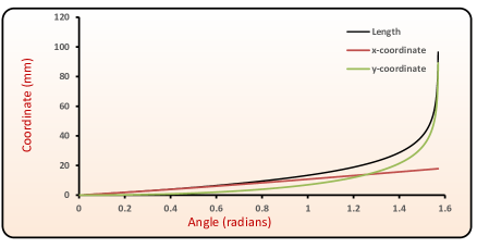
Figure 26: X,Y and S as function of angle $\theta$.

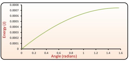
Figure 27: Bending energy U_net as a function of angle $\theta$.

4.3 Lap-Shear Testing

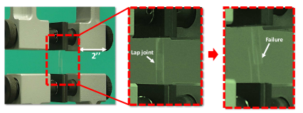
Figure 28: Lap shear-strength test specimen in tensile tester.

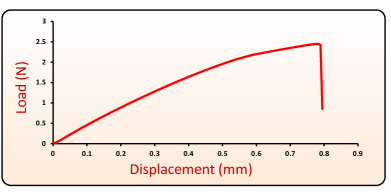
Figure 29: Force versus displacement curve during lap shear-strength testing. For this specimen a nominal plastic strain of 9.0% was imposed and the shear-strength ($\sigma_{s}$=F_max/A) was estimated to be 0.07 MPa.

Preparation of lap specimens and shear-strength measurements were carried out in Instron testing machine. A lap joint was assembled between two film layers, each layer being nearly 100 $\mu$m thick. The overlapping region was nearly $A=5x5=25$ mm² in area. A cross-head speed of 0.5 mm/min was chosen to apply desired compression load on the overlapping area. The sample was plastically bonded by pressing between two parallel (accuracy: 1 $\mu$m) flats. Lap joint was tested for shear-strength in tension mode (at a cross-head speed of 15 mm/min). A snapshot of the test is shown in Figure  28. The peak force before failure divided by the bonded area was taken as the lap shear-strength. Figure  29 shows the force versus displacement during a lap shear-strength measurement.

4.4 Mechanics of ‘hydrostatic die’

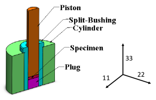
Figure 30: A set-up to achieve near hydrostatic compression.

As discussed in the main letter and Supplementary video S2, the purpose of designing a ‘hydrostatic die’ was to explicitly show the role of active plastic deformation in achieving sub-T_g, solid-state, plasticity-induced bonding. Figure  30 shows the CAD model of a ‘hydrostatic die’. Such a setup is capable of generating large levels of hydrostatic pressure, while strongly limiting the plastic flow to negligible levels, when a circular stack of film with a radius equal to the internal radius of the cavity is compressed inside the die.

We present a couple of analyses to demonstrate the principle of the ‘hydrostatic die’. Illustrations related to deformation theory of plasticity, as presented here, are borrowed in parts from [35, 39]. In what follows next, a boldface letter is to used to indicate a tensor variable.

4.4.1 Elasticity Analysis

First, we consider axisymmetric elastic compression of a film stack placed in the die. Here, all strains are assumed to be elastic and frictional forces are assumed to be absent. The solution to this problem is derived from the standard procedure of stresses in a thick-walled cylinder with a zero internal radius. A cylindrical coordinate system (r, $\Theta$, z) is used. The principal stress components are denoted by $\sigma_{r}$, $\sigma_{\Theta}$ and $\sigma_{z}$, and the associated strains given as $\epsilon_{r}$, $\epsilon_{\Theta}$ and $\epsilon_{z}$. All other shear components are zero. Due to axisymmetry and wall constraints inside the die we have $\sigma_{r}=\sigma_{\Theta}$ ($=\sigma$, say) and $\epsilon_{r}=\epsilon_{\Theta}=0$. Using the boundary constraints with the stress-strain relation of linear elasticity:

$$\boldsymbol{\epsilon}=\frac{1+\nu}{E}\boldsymbol{\sigma}-\frac{\nu}{E}tr(\boldsymbol{\sigma})\mathbf{I},$$ (33)

we find,

$$\sigma_{z}=\frac{E(1-\nu)\epsilon_{z}}{(1-2\nu)(1+\nu)}$$ (34)

$$\sigma=\frac{E\nu\epsilon_{z}}{(1-2\nu)(1+\nu)}$$ (35)

where, $E$ and $\nu$ are Young’s modulus and Poisson’s ratio, respectively. The stress tensor in terms of principal directions $\bar{e}_{r}$, $\bar{e}_{\Theta}$ and $\bar{e}_{z}$ is given as $\boldsymbol{\sigma}$ $=$ $\sigma$ $\bar{e}_{r}\otimes\bar{e}_{r}$ + $\sigma$ $\bar{e}_{\Theta}\otimes\bar{e}_{\Theta}$ + $\sigma_{z}$ $\bar{e}_{z}\otimes\bar{e}_{z}$. $\boldsymbol{\sigma}$ can be decomposed into deviatoric part ($\boldsymbol{\sigma}^{\prime}$) and hydrostatic part (${\sigma_{m}\mathbf{I}}$, with $\sigma_{m}=(\sigma_{r}+\sigma_{\Theta}+\sigma_{z})/3$ denoting the mean normal stress), and written as $\boldsymbol{\sigma}$ = $\boldsymbol{\sigma}^{\prime}$ + $\sigma_{m}\mathbf{I}$. In the present scenario:

$$\boldsymbol{\sigma}^{\prime}=\left(\begin{array}[]{lccc}\frac{\sigma-\sigma_{z}}{3}&0&0\\ 0&\frac{\sigma-\sigma_{z}}{3}&0\\ 0&0&\frac{2(\sigma_{z}-\sigma)}{3}\end{array}\right)$$

$$\sigma_{m}\mathbf{I}=\left(\begin{array}[]{ccc}\frac{2\sigma+\sigma_{z}}{3}&0&0\\ 0&\frac{2\sigma+\sigma_{z}}{3}&0\\ 0&0&\frac{2\sigma+\sigma_{z}}{3}\end{array}\right)$$

The von Mises stress ($\sigma_{v}$) is given as:

$$\sigma_{v}=\sqrt{\frac{3}{2}\boldsymbol{\sigma}^{\prime}:\boldsymbol{\sigma}^{\prime}}$$ (36)

Thus, in the presence of die the von Mises stress ($\sigma_{v,die}$) and hydrostatic pressure ($p_{die}=-\sigma_{m}$) are given as:

$$p_{die}=\frac{E|\epsilon_{z}|}{3(1-2\nu)}$$ (37)

$$\sigma_{v,die}=\frac{E|\epsilon_{z}|}{1+\nu}$$ (38)

In contrast if we imagined axisymmetric, unconstrained elastic compression, without any frictional effects then we would have $\sigma_{z}=E\epsilon_{z}$, and $\sigma_{r}=\sigma_{\Theta}=0$. In such case the von Mises stress ($\sigma_{v,no-die}$) and hydrostatic pressure ($p_{no-die}$) would be given as:

$$p_{no-die}=\frac{E|\epsilon_{z}|}{3}$$ (39)

$$\sigma_{v,no-die}=|\sigma_{z}|$$ (40)

We emphasize that elasticity analysis is valid only up to the onset of plastic deformation. However, if we are within the elastic limit then equations  37 and  39 show that large hydrostatic-pressure can build up during compression inside the die. Particularly in the limit as $\nu\to 0.5$, $p_{die}$ $\to$ $\infty$.

In the video S2, a maximum compressive load of $40$ kN is applied on a film-stack with radius $0.5^{\prime\prime}=$ 12.5 mm; corresponding to $\sigma_{z}=-78.98$ MPa. According to equation  34, if $\sigma_{z}=-78.98$ MPa, $\nu=0.4$, and E=300 MPa then $\epsilon_{z}$ works out to be $-0.12$. Substituting $|\epsilon_{z}|=0.12$, $E=300$ MPa and $\nu=0.4$ in equation  38, $\sigma_{v,die}=25.7$ MPa. Clearly, $\sigma_{v,die}$ thus obtained is larger than the yield strength of the film. This indicates the possibility of plastic deformation even in the presence of the die. Next, we present an analysis based on the incremental (or “flow theory”) of plasticity, which accounts for plastic deformation.

4.4.2 Incremental (“Flow Theory”) of Plasticity

Here, we take into account the plastic deformation and demonstrate how little amount of plastic straining occurs when a film stack is compressed in the presence of the ‘hydrostatic die’.

According to the total deformation analysis, the total strain increment tensor ($d\boldsymbol{\epsilon}$) is the sum of the elastic strain increment tensor ($d\boldsymbol{\epsilon}^{e}$) and the plastic strain increment tensor ($d\boldsymbol{\epsilon}^{p}$):

$$d\boldsymbol{\epsilon}=d\boldsymbol{\epsilon}^{e}+d\boldsymbol{\epsilon}^{p}$$ (41)

The increment in elastic strain tensor can be derived using equation  33 and written as:

$$d\boldsymbol{\epsilon}^{e}=\frac{1+\nu}{E}d\boldsymbol{\sigma}^{\prime}+\frac{1-2\nu}{E}d(tr(\boldsymbol{\sigma}))\mathbf{I}$$ (42)

Under multi-axial loading the behavior of ductile materials can be described by the Levy-Mises equations, which relate the principal components of strain increments in plastic deformation to the principal applied stresses. In the present scenario this can be expressed as:

$$\frac{\dot{\epsilon_{r}}^{p}}{\sigma_{r}^{\prime}}=\frac{\dot{\epsilon_{\Theta}}^{p}}{\sigma_{\Theta}^{\prime}}=\frac{\dot{\epsilon_{z}}^{p}}{\sigma_{z}^{\prime}}$$ (43)

On the grounds of axisymmetric compression, similar to what was discussed in the previous section, we have $\sigma_{r}=\sigma_{\Theta}$ ($=\sigma$, say), and therefore $\dot{\epsilon}_{r}=\dot{\epsilon}_{\Theta}$ ($\dot{\epsilon}$, say). If we consider small intervals of time $dt$ and call the resultant changes in normal plastic strains as $d\epsilon_{r}^{p}=d\epsilon_{\Theta}^{p}$ ($=d\epsilon^{p}$) and $d\epsilon_{z}^{p}$, it follows that:

$$d\epsilon^{p}=\sigma^{\prime}d\lambda$$ (44)

$$d\epsilon_{z}^{p}=\sigma_{z}^{\prime}d\lambda$$ (45)

here, $d\lambda$ is an instantaneous non-negative constant of proportionality which may vary throughout a straining programme. We further define following quantities to aid this illustration:

$$|\boldsymbol{\sigma^{\prime}}|=\sqrt{\boldsymbol{\sigma^{\prime}}:\boldsymbol{\sigma^{\prime}}}$$ (46)

$$\bar{\sigma}=\sqrt{\frac{3}{2}\boldsymbol{\sigma^{\prime}}:\boldsymbol{\sigma^{\prime}}}=\sqrt{\frac{3}{2}}|\boldsymbol{\sigma^{\prime}}|$$ (47)

$$|d\boldsymbol{\epsilon}^{p}|=\sqrt{d\boldsymbol{\epsilon}^{p}:d\boldsymbol{\epsilon}^{p}}$$ (48)

$$d\bar{\epsilon}^{p}=\sqrt{\frac{2}{3}d\boldsymbol{\epsilon}^{p}:d\boldsymbol{\epsilon}^{p}}=\sqrt{\frac{2}{3}}|d\boldsymbol{\epsilon^{p}|}$$ (49)

The flow rule can be written as:

$$\frac{d\boldsymbol{\epsilon}^{p}}{|d\boldsymbol{\epsilon}^{p}|}=\frac{\boldsymbol{\sigma^{\prime}}}{|\boldsymbol{\sigma}^{\prime}|}$$ (50)

If we assume that plastic flow is incompressible then the total increment in plastic strain can be written as:

$$d\boldsymbol{\epsilon}^{p}=-\frac{1}{2}d\epsilon_{z}^{p}\bar{e_{r}}\otimes\bar{e_{r}}-\frac{1}{2}d\epsilon_{z}^{p}\bar{e}_{\Theta}\otimes\bar{e}_{\Theta}+d\epsilon_{z}^{p}\bar{e_{z}}\otimes\bar{e_{z}}$$ (51)

It is worth noting that at any instance neither the directions nor the relative magnitudes of plastic strain components change, and therefore we can write equation  51 as:

$$\boldsymbol{\epsilon}^{p}=-\frac{1}{2}\epsilon_{z}^{p}\bar{e_{r}}\otimes\bar{e_{r}}-\frac{1}{2}\epsilon_{z}^{p}\bar{e}_{\Theta}\otimes\bar{e}_{\Theta}+\epsilon_{z}^{p}\bar{e_{z}}\otimes\bar{e_{z}}$$ (52)

By choosing $\boldsymbol{D}=-\frac{1}{2}\bar{e_{r}}\otimes\bar{e_{r}}-\frac{1}{2}\bar{e}_{\Theta}\otimes\bar{e}_{\Theta}+\bar{e_{z}}\otimes\bar{e_{z}}$, we can re-write equation  51 as:

$$\boldsymbol{\epsilon}^{p}=\epsilon_{z}^{p}\boldsymbol{D}$$ (53)

In equation  53, $\epsilon_{z}^{p}$ is negative during compression. Using the flow rule from equation  50, and the fact that increments in plastic strains are proportional to the principal directions (which are constant throughout the deformation history); we can rewrite flow rule in terms of total plastic strain at any instant as:

$$\frac{\boldsymbol{\epsilon}^{p}}{|\boldsymbol{\epsilon}^{p}|}=\frac{\boldsymbol{\sigma}^{\prime}}{|\boldsymbol{\sigma}^{\prime}|}$$ (54)

If we assume plastic deformation to continue at a constant yield $Y$, then:

$$Y=\sqrt{\frac{3}{2}}|\boldsymbol{\sigma}^{\prime}|$$ (55)

It is worth mentioning that the yield strength of polymers is usually a function of hydrostatic pressure and plastic strain (and the flow stress increases with increasing hydrostatic pressure and plastic strain, thus an assumption of constant yield stress is an under estimation).

By combining equations  53,  54 and  55 we can write:

$$\boldsymbol{\sigma}^{\prime}=\frac{\epsilon_{z}^{p}}{|\epsilon_{z}^{p}|}\frac{2}{3}Y\boldsymbol{D}$$ (56)

Since $\epsilon_{z}^{p}$ is negative during compression, equation  57 can be re-written as:

$$\boldsymbol{\sigma}^{\prime}=-\frac{2}{3}Y\boldsymbol{D}$$ (57)

The elastic strain increments, as given in equation  42, occur both due to deviatoric stress and hydrostatic stress. At the onset of plastic flow (and continued plastic yielding at constant flow stress) the the deviatoric stress becomes constant (given by equation  57), after which there is no further contribution to elastic strains due to deviatoric stress components. However, the normal stress and the hydrostatic part of the elastic strains continue to increase. Thus, total elastic-strain can be written as:

$$\boldsymbol{\epsilon}^{e}=-(\frac{1+\nu}{E})(\frac{2Y}{3})\boldsymbol{D}+\frac{{\sigma}_{m}}{3}(\frac{1-2\nu}{E})\mathbf{I}$$ (58)

From equation  41, the total strain can be written as:

$$\boldsymbol{\epsilon}=\epsilon_{z}^{p}\boldsymbol{D}-(\frac{1+\nu}{E})(\frac{2Y}{3})\boldsymbol{D}+\frac{{\sigma}_{m}}{3}(\frac{1-2\nu}{E})\mathbf{I}$$ (59)

Now imposing the constraint that total strains in the $r$ and $\Theta$ direction are zero i.e. $\epsilon_{r}=\epsilon_{\Theta}=0$ then equation  59 implies:

$$\frac{\sigma_{m}}{3}=\frac{E}{1-2\nu}[\frac{\epsilon_{z}^{p}}{2}-\frac{Y(1+\nu)}{3E}]$$ (60)

Thus, the overall stress tensor can be written as:

$$\boldsymbol{\sigma}=-\frac{2Y}{3}\boldsymbol{D}+\frac{E}{2(1-2\nu)}\epsilon_{z}^{p}\mathbf{I}-\frac{Y(1+\nu)}{3(1-2\nu)}\mathbf{I}$$ (61)

If we choose values same as in the previous section, we get $|\epsilon_{z}^{p}|$ nearly $2\%$. We emphasize the fact that in polymers the plastic straining is accompanied with hardening, and the yield stress increases with mean normal pressure, therefore, $|\epsilon_{z}^{p}|$ = 2% is quite an overestimation. Lastly, the ratio $\frac{\sigma_{r}}{\sigma_{z}}=0.96$ which suggests that the state of stress inside the die is ‘hydrostatic’.

These calculations demonstrate that despite the large hydrostatic pressures there is only small plastic straining, due to which no bonding outcome is noted.

4.5 Mechanics of Axisymmetric Upseting

Unconstrained compression of film stack with initial thickness much smaller than the radius of the stack qualifies as a classic case of an upsetting problem. As shown in the Supplementary video S2, a film stack with an initial thickness of $0.84$ mm requires peak loads up to 40 kN (which equates to a peak nominal stress of 78.9 MPa, much larger than yield strength of the polymer) in order to achieve a final thickness of $0.70$ mm due to compression. This can be attributed to frictional forces acting on the top and the bottom surfaces during compression.

Figure  31 schematically shows the upsetting of a film stack. Figure 32 shows the stress components along with the frictional forces acting on a cylindrical element. Now, we estimate the loads required to achieve plastic deformation in upsetting scenario and their comparison with the experimentally noted loads.

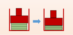
Figure 31: Axisymmetric Upsetting of laminates.

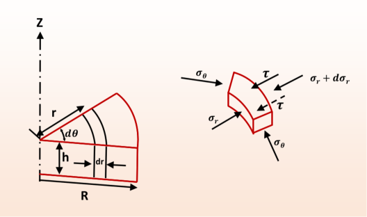
Figure 32: Stresses and frictional forces acting on an element during axisymmetric upsetting.

Upper Bound Analysis for Load Estimation

Upper bound analysis is one of the methods to estimate the deformation load and the average forming or forging pressure. The analysis presented here is borrowed from [6, 39]. The usual assumptions are:

1. The deforming material is isotropic and incompressible.

2. The elastic deformations of the material (and tool) are neglected. The tool is essentially rigid, and material behavior is perfect-rigid-plastic.

3. The inertial forces are small and are neglected.

4. The frictional shear stress, $\tau$, is constant at the die/material interface and is defined as $\tau=f\bar{\sigma}=m\bar{\sigma}/\sqrt{3}$.

5. The material flows according to the von Mises flow rule.

6. The flow stress and the temperature are constant within the analyzed portion of the deforming material.

In addition, following steps are key to invoking the upper bound analysis:

7. Description of a family of admissible fields (using parameters to be determined later); these must satisfy the conditions of: incompressibility, continuity, and velocity boundaries.

8. Calculation for the energy rates of deformation, internal shear, and friction shear.

9. Calculation for the total energy rate and minimization with respect to unknown parameters of velocity field formulation.

One of the simplest solutions to upset forging assumes that a decrease in specimen height is compensated by an increase in width or radius without any bulging or barreling. This implies that a rectangular solid deforms to a thinner and wider rectangular piece. In an axisymmetric scenario, cylindrical solids retain their cylindrical geometry. Since the lines parallel to the height axis remain parallel, a parallel velocity field is assumed. A similar assumption on the velocity field is also made here, along with homogeneous deformation.

Velocity and Strain Rates

In order to estimate loads, first we need to calculate the velocity field and strain-rates. During upsetting, as shown in Figure  31, we have already assumed that the volume is constant during the plastic flow i.e. the volume of the material moved in the z direction is equal to that moved in the radial direction (shortly we shall also impose plastic incompressibility during calculation of strain rates):

$$\pi r^{2}V_{D}=2\pi rv_{r}h$$

or,

$$v_{r}=V_{D}r/2h$$ (62)

In the z-direction, $v_{z}$ can be considered to vary linearly while satisfying the boundary conditions at $z=0$ and $z=h$. In the tangential direction, $\Theta$, there is no flow (due to symmetry). Thus:

$$v_{z}=-V_{D}z/h$$ (63)

From the Figure  32, the increase in strain in $\Theta$ direction, i.e., the length of the arc, is given by:

$$d\epsilon_{\Theta}=\frac{(r+dr)d\Theta-rd\Theta}{rd\Theta}=\frac{dr}{r}$$ (64)

thus, the strain rate is

$${\dot{\epsilon}_{\Theta}}=\frac{d\epsilon_{\Theta}}{dt}=\frac{dr}{dt}\frac{1}{r}=\frac{v_{r}}{r}=\frac{V_{D}}{2h}$$ (65)

The other strain rates are:

$${\dot{\epsilon}_{z}}=\frac{\partial v_{z}}{\partial z}=\frac{-V_{D}}{h}$$ (66)

$${\dot{\epsilon}_{r}}=\frac{\partial v_{r}}{\partial r}=\frac{V_{D}}{2h}={\dot{\epsilon}_{\Theta}}$$ (67)

$$\dot{\gamma}_{rz}=\left(\frac{\partial v_{r}}{\partial z}+\frac{\partial v_{z}}{\partial r}\right)=0$$ (68)

$$\dot{\gamma}_{\Theta z}=\dot{\gamma}_{\Theta r}=0$$ (69)

Thus, the effective strain rate is:

$${\dot{\bar{\epsilon}}}=\sqrt{\frac{2}{3}(\dot{\epsilon}^{2}_{\Theta}+\dot{\epsilon}^{2}_{r}+\dot{\epsilon}^{2}_{z})}=|\dot{\epsilon}_{z}|$$ (70)

The strains can be obtained by integrating the strain rates with respect to time, i.e.:

$$\epsilon_{z}=\int^{t}_{t_{o}}\dot{\epsilon}_{z}dt=-\int^{t}_{t_{o}}\frac{V_{D}dt}{h}$$ (71)

or with $dh=-V_{D}dt$:

$$\epsilon_{z}=\int^{h}_{h_{o}}\frac{dh}{h}=ln\frac{h}{h_{o}}$$ (72)

Similarly, the other strains can be obtained as:

$$\epsilon_{\Theta}=\epsilon_{r}=\frac{1}{2}ln\frac{h}{h_{o}}=-\frac{\epsilon_{z}}{2}$$ (73)

The effective strain is

$$\bar{\epsilon}=|\epsilon_{z}|$$ (74)

Upper Bound Analysis

In the upper bound analysis, the load is obtained by equating the rate of work done by the tool with the upper bound estimate of energy expended due to deforming material:

If $\dot{E}_{T}$ is the total energy rate expended due to material deformation, then $\dot{E}_{T}=L\times V$ [10], here L represents the forming load and V represents the velocity of the die.

The total energy expended in material deformation itself can be expressed as sum of energy rates for deformation ($\dot{E}_{D}$), internal shear ($\dot{E}_{S}$) and friction ($\dot{E}_{F}$):

$$\dot{E}_{T}=\dot{E}_{D}+\dot{E}_{S}+\dot{E}_{F}$$

or,

$$\dot{E}_{T}=\int_{V}\bar{\sigma}\dot{\bar{\epsilon}}dV+\int_{SS}\tau|\triangle v|ds+\int_{SF}\tau_{i}v_{i}ds$$ (75)

where, $v$ is the relative velocity between the two zones of material when the velocity has internal shear surfaces and $\tau=\bar{\sigma}/\sqrt{3}$; $S$ indicates surface (internal or at die/material interface), $v_{i}$ is the die material interface velocity in the “i” portion of the deforming material and $\tau_{i}=m_{i}\bar{\sigma}/\sqrt{3}$ which is the interface shear stress at the “i” portion of the deforming material. $m$ is chosen as 1 for the upper bound analysis here.

The velocity field for homogeneous upsetting has been calculated before and a constant flow stress ($\bar{\sigma}$) is assumed. The deformation energy rate is given as:

$$\dot{E}_{D}=\int_{V}\bar{\sigma}\dot{\bar{\epsilon}}dV=h\pi R^{2}\bar{\sigma}\frac{V_{D}}{h}$$ (76)

$\dot{E}_{S}$ (internal shear energy rate) = 0, because there are no internal velocity discontinuities in the assumed homogeneous velocity field.

The friction energy rate is given as:

$$\dot{E}_{F}=2\int_{SF}\tau_{i}v_{i}ds$$

where $v_{i}$ is the radial velocity given by equation  62, and $ds=2\pi rdr$. $\dot{E}_{F}$ includes the friction energies on both the top and bottom surfaces of the deforming part. Thus,

$$\dot{E}_{F}=2\int_{0}^{R}\tau_{i}\frac{V_{D}}{2h}r2\pi rdr=\frac{4\pi\tau_{i}V_{D}}{2h}\int_{0}^{R}r^{2}dr$$ (77)

or, with $\tau=m\bar{\sigma}/\sqrt{3}$,

$$\dot{E}_{F}=\frac{2}{3}\pi m\frac{\bar{\sigma}}{\sqrt{3}}\frac{V_{D}}{h}R^{3}$$ (78)

Thus, total energy rate is given as:

$$\dot{E}_{T}=\pi R^{2}\bar{\sigma}V_{D}+\frac{2}{3}\pi m\frac{\bar{\sigma}}{\sqrt{3}}\frac{V_{D}}{h}R^{3}$$

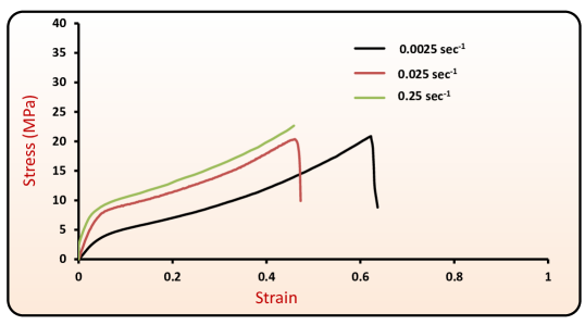
Figure 33: Strain-rate sensitivity of E3/E15 in 1:1-42.3% PEG. Nominal strain-rates are listed.

and, the load is estimated as:

$$L=\frac{\dot{E}_{T}}{V_{D}}=\pi R^{2}\bar{\sigma}\left(1+\frac{2}{3\sqrt{3}}m\frac{R}{h}\right)$$ (79)

If we set $R=12.7$ $mm$, $h=0.7$$mm$, $\bar{\sigma}=10$ MPa, we estimate the $L=40.414$ $kN$. As shown in the upsetting video S2 (unconstrained case), $t_{o}=0.84$ $mm$, $t_{f}=0.7$ $mm$ and therefore $e=ln(t_{o}/t_{f})$ $0.18$. Duration of the loading is approximately 30 seconds, and we use a flow stress value $\bar{\sigma}=10$ MPa (for an estimated strain rate of 0.006 sec^-1) from Figure  33 (which shows strain-rate sensitivity measurements in tension).

References

- [1] http://storage.dow.com.edgesuite.net/pharmaandfood-dow-com/pharma/Pharma_METHOCEL_Comparison_Table.pdf.
- [2] Methocel cellulose ethers in aqueous systems for tablet coating. http://www.dow.com/scripts/litorder.asp?filepath=/198-00755.pd.
- [3] Methocel molecular weight viscosity relationship. http://dowwolff.custhelp.com/app/answers/detail/a_id/1316.
- [4] Segmental and chain dynamics in amorphous polymers. http://comse.chemeng.ntua.gr/segmdyn_polpage.htm.
- [5] A Alegria, E Guerrica-Echevarria, L Goitiandia, I Telleria, and J Colmenero. . alpha.-relaxation in the glass transition range of amorphous polymers. 1. temperature behavior across the glass transition. Macromolecules, 28(5):1516–1527, 1995.
- [6] Taylan Altan, Gracious Ngaile, and Gangshu Shen. Cold and hot forging: fundamentals and applications, volume 1. ASM international, 2005.
- [7] C Austin Angell, Kia L Ngai, Greg B McKenna, Paul F McMillan, and Steve W Martin. Relaxation in glassforming liquids and amorphous solids. Journal of Applied Physics, 88(6):3113–3157, 2000.
- [8] Ali S Argon. The physics of deformation and fracture of polymers. Cambridge University Press, 2013.
- [9] AS Argon, RE Cohen, and AC Patel. A mechanistic model of case ii diffusion of a diluent into a glassy polymer. Polymer, 40(25):6991–7012, 1999.
- [10] B Avitzur. Metal forming: processes and analysis, 1968.
- [11] Craig R Bartels, Buckley Crist, and William W Graessley. Self-diffusion coefficient in melts of linear polymers: chain length and temperature dependence for hydrogenated polybutadiene. Macromolecules, 17(12):2702–2708, 1984.
- [12] Yuri M Boiko. On the formation of topological entanglements during the contact of glassy polymers. Colloid and Polymer Science, 290(12):1201–1206, 2012.
- [13] Yuri M Boiko. Is adhesion between amorphous polymers sensitive to the bulk glass transition? Colloid and Polymer Science, 291(9):2259–2262, 2013.
- [14] Yuri M Boiko and Robert E Prud’Homme. Strength development at the interface of amorphous polymers and their miscible blends, below the glass transition temperature. Macromolecules, 31(19):6620–6626, 1998.
- [15] Yuri M Boiko, Vladimir A Zakrevskii, and Vladimir A Pakhotin. Chain scission upon fracture of autoadhesive joints formed from glassy poly (phenylene oxide). The Journal of Adhesion, 90(7):596–606, 2014.
- [16] Maurice Brogly, Ahmad Fahs, and Sophie Bistac. Assessment of nanoadhesion and nanofriction properties of formulated cellulose-based biopolymers by afm. In Bharat Bhushan, editor, Scanning Probe Microscopy in Nanoscience and Nanotechnology 2, NanoScience and Technology, pages 473–504. Springer Berlin Heidelberg, 2011.
- [17] HR Brown. The adhesion between polymers. Annual Review of Materials Science, 21(1):463–489, 1991.
- [18] F Bueche. Viscosity, self-diffusion, and allied effects in solid polymers. The Journal of Chemical Physics, 20(12):1959–1964, 1952.
- [19] FWMP Bueche, WM Cashin, and P Debye. The measurement of self-diffusion in solid polymers. The Journal of Chemical Physics, 20(12):1956–1958, 1952.
- [20] Franco M Capaldi, Mary C Boyce, and Gregory C Rutledge. Molecular response of a glassy polymer to active deformation. Polymer, 45(4):1391–1399, 2004.
- [21] Bum-Rae Cho and John L Kardos. Consolidation and self-bonding in poly (ether ether ketone)(peek). Journal of applied polymer science, 56(11):1435–1454, 1995.
- [22] Ralph H Colby. Dynamic scaling approach to glass formation. Physical Review E, 61(2):1783, 2000.
- [23] Costantino Creton, Edward J Kramer, Hugh R Brown, and Chung-Yuen Hui. Adhesion and fracture of interfaces between immiscible polymers: from the molecular to the continuum scale. In Molecular Simulation Fracture Gel Theory, pages 53–136. Springer, 2002.
- [24] P.-G. De Gennes. The formation of polymer/polymer junctions. Tribology Series, 7:355–367, 1981.
- [25] P.-G. de Gennes. Tension superficielle des polymères fondus. Comptes rendus de l’Académie des sciences. Série 2, Mécanique, Physique, Chimie, Sciences de l’univers, Sciences de la Terre, 307(18):1841–1844, 1988.
- [26] P.-G. de Gennes. In Isaac C Sanchez and Lee E Fitzpatrick, editors, Physics of polymer surfaces and interfaces. Butterworth-Heinemann Boston, 1992.
- [27] P.-G. de Gennes. Soft interfaces: the 1994 Dirac memorial lecture. Cambridge University Press, 2005.
- [28] Pablo G Debenedetti and Frank H Stillinger. Supercooled liquids and the glass transition. Nature, 410(6825):259–267, 2001.
- [29] M Doxastakis, DN Theodorou, G Fytas, F Kremer, R Faller, F Müller-Plathe, and N Hadjichristidis. Chain and local dynamics of polyisoprene as probed by experiments and computer simulations. The Journal of chemical physics, 119(13):6883–6894, 2003.
- [30] MD Ediger, CA Angell, and Sidney R Nagel. Supercooled liquids and glasses. The journal of physical chemistry, 100(31):13200–13212, 1996.
- [31] Henry Eyring. Viscosity, plasticity, and diffusion as examples of absolute reaction rates. The Journal of chemical physics, 4(4):283–291, 2004.
- [32] Z Fakhraai and JA Forrest. Measuring the surface dynamics of glassy polymers. Science, 319(5863):600–604, 2008.
- [33] Gerald Fleischer. Temperature dependence of self diffusion of polystyrene and polyethylene in the melt an interpretation in terms of the free volume theory. Polymer Bulletin, 11(1):75–80, 1984.
- [34] Gerald Fleischer and Matthias Appel. Chain length and temperature dependence of the self-diffusion of polyisoprene and polybutadiene in the melt. Macromolecules, 28(21):7281–7283, 1995.
- [35] Morton E Gurtin, Eliot Fried, and Lallit Anand. The mechanics and thermodynamics of continua. Cambridge University Press, 2010.
- [36] John M Hutchinson. Physical aging of polymers. Progress in Polymer Science, 20(4):703–760, 1995.
- [37] B Jerome and J Commandeur. Dynamics of glasses below the glass transition. Nature, 386:589–592, 1997.
- [38] Kenneth Langstreth Johnson. Contact mechanics. Cambridge university press, 1987.
- [39] William Johnson and Peter Bassindale Mellor. Engineering plasticity. Horwood, 1983.
- [40] RAL. Jones. Interfaces. In Robert Nobbs Haward and Robert Joseph Young, editors, The physics of glassy polymers. Springer, 1997.
- [41] K Jud and HH Kausch. Load transfer through chain molecules after interpenetration at interfaces. Polymer Bulletin, 1(10):697–707, 1979.
- [42] K Jud, HH Kausch, and JG Williams. Fracture mechanics studies of crack healing and welding of polymers. Journal of Materials Science, 16(1):204–210, 1981.
- [43] H. H. Kausch and M Tirrell. Polymer interdiffusion. Annual Review of Materials Science, 19:341–377, 1989.
- [44] CM Keary. Characterization of methocel cellulose ethers by aqueous sec with multiple detectors. Carbohydrate polymers, 45(3):293–303, 2001.
- [45] Kyung Suk Kim and N Aravas. Elastoplastic analysis of the peel test. International Journal of Solids and Structures, 24(4):417–435, 1988.
- [46] R Kimmich, W Unrath, G Schnur, and E Rommel. Nmr measurement of small self-diffusion coefficients in the fringe field of superconducting magnets. Journal of Magnetic Resonance (1969), 91(1):136–140, 1991.
- [47] Jacob Klein. Interdiffusion of polymers. Science, 250(4981):640–646, 1990.
- [48] DB Kline and RP Wool. Polymer welding relations investigated by a lap shear joint method. Polymer Engineering & Science, 28(1):52–57, 1988.
- [49] Kazimierz Krynicki, Christopher D Green, and David W Sawyer. Pressure and temperature dependence of self-diffusion in water. Faraday Discussions of the Chemical Society, 66:199–208, 1978.
- [50] K Kunz and M Stamm. Initial stages of interdiffusion of pmma across an interface. Macromolecules, 29(7):2548–2554, 1996.
- [51] Hau-Nan Lee, Keewook Paeng, Stephen F Swallen, and MD Ediger. Direct measurement of molecular mobility in actively deformed polymer glasses. Science, 323(5911):231–234, 2009.
- [52] Lieng-Huang Lee. Adhesion of high polymers. i. influence of diffusion, adsorption, and physical state on polymer adhesion. Journal of Polymer Science Part A-2: Polymer Physics, 5(4):751–760, 1967.
- [53] Lieng-Huang Lee. Fundamentals of adhesion. Springer, 1991.
- [54] Leslie S Loo, Robert E Cohen, and Karen K Gleason. Chain mobility in the amorphous region of nylon 6 observed under active uniaxial deformation. Science, 288(5463):116–119, 2000.
- [55] Kevin F Mansfield and Doros N Theodorou. Molecular dynamics simulation of a glassy polymer surface. Macromolecules, 24(23):6283–6294, 1991.
- [56] Marie K Mapes, Stephen F Swallen, and MD Ediger. Self-diffusion of supercooled o-terphenyl near the glass transition temperature. The Journal of Physical Chemistry B, 110(1):507–511, 2006.
- [57] Anne M Mayes. Glass transition of amorphous polymer surfaces. Macromolecules, 27(11):3114–3115, 1994.
- [58] Gregory F Meyers, Benjamin M DeKoven, and Jerry T Seitz. Is the molecular surface of polystyrene really glassy? Langmuir, 8(9):2330–2335, 1992.
- [59] Nikhil Padhye. Continous Forming and Sub-Tg, Solid-State, Plasticity-Induced Bonding of Polymeric Films. PhD thesis, Massachusetts Institute of Technology, Cambridge, 2015.
- [60] Nikhil Padhye, David M. Parks, Alexander H. Slocum, and Bernhardt L. Trout. An enhanced accuracy t-peel test for vertical test machines. 2015.
- [61] DS Pearson, G Ver Strate, E Von Meerwall, and FC Schilling. Viscosity and self-diffusion coefficient of linear polyethylene. Macromolecules, 20(5):1133–1141, 1987.
- [62] Stephen Prager and Matthew Tirrell. The healing process at polymer–polymer interfaces. The journal of chemical physics, 75(10):5194–5198, 1981.
- [63] R Richert and K Samwer. Enhanced diffusivity in supercooled liquids. New Journal of Physics, 9(2):36, 2007.
- [64] Sunanda Roy, CY Yue, ZY Wang, and L Anand. Thermal bonding of microfluidic devices: Factors that affect interfacial strength of similar and dissimilar cyclic olefin copolymers. Sensors and Actuators B: Chemical, 161(1):1067–1073, 2012.
- [65] Spencer D Schaber, Dimitrios I Gerogiorgis, Rohit Ramachandran, James MB Evans, Paul I Barton, and Bernhardt L Trout. Economic analysis of integrated continuous and batch pharmaceutical manufacturing: a case study. Industrial & Engineering Chemistry Research, 50(17):10083–10092, 2011.
- [66] R Scott Smith and Bruce D Kay. Breaking through the glass ceiling: Recent experimental approaches to probe the properties of supercooled liquids near the glass transition. The Journal of Physical Chemistry Letters, 3(6):725–730, 2012.
- [67] Frank H Stillinger. A topographic view of supercooled liquids and glass formation. Science, 267(5206):1935–1939, 1995.
- [68] IA Strelnikov, NK Balabaev, MA Mazo, and EF Oleinik. Analysis of local rearrangements in chains during simulation of the plastic deformation of glassy polymethylene. Polymer Science Series A, 56(2):219–227, 2014.
- [69] Stephen F Swallen, Osamu Urakawa, Marie Mapes, and MD Ediger. Self-diffusion and spatially heterogeneous dynamics in supercooled liquids near tg. In SLOW DYNAMICS IN COMPLEX SYSTEMS: 3rd International Symposium on Slow Dynamics in Complex Systems, volume 708, pages 491–495. AIP Publishing, 2004.
- [70] SS Voyutskii and VL Vakula. The role of diffusion phenomena in polymer-to-polymer adhesion. Journal of Applied Polymer Science, 7(2):475–491, 1963.
- [71] Junichiro Washiyama, Edward J Kramer, Costantino F Creton, and Chung-Yuen Hui. Chain pullout fracture of polymer interfaces. Macromolecules, 27(8):2019–2024, 1994.
- [72] R. P. Wool. Polymer Interfaces: Surface and Strength. Hanser Press: New York, 1995.
- [73] RP Wool and KM O’connor. A theory crack healing in polymers. Journal of Applied Physics, 52(10):5953–5963, 1981.
- [74] Q-Y Zhou, AS Argon, and RE Cohen. Enhanced case-ii diffusion of diluents into glassy polymers undergoing plastic flow. Polymer, 42(2):613–621, 2001.