Entangling superconducting qubits in a multi-cavity system

Abstract

Important tasks in cavity quantum electrodynamics include the generation and control of quantum states of spatially-separated particles distributed in different cavities. An interesting question in this context is how to prepare entanglement among particles located in different cavities, which are important for large-scale quantum information processing. We here consider a multi-cavity system where cavities are coupled to a superconducting (SC) qubit and each cavity hosts many SC qubits. We show that all intra-cavity SC qubits plus the coupler SC qubit can be prepared in an entangled Greenberger-Horne-Zeilinger (GHZ) state, by using a single operation and without the need of measurements. The GHZ state is created without exciting the cavity modes; thus greatly suppressing the decoherence caused by the cavity-photon decay and the effect of unwanted inter-cavity crosstalk on the operation. We also introduce two simple methods for entangling the intra-cavity SC qubits in a GHZ state. As an example, our numerical simulations show that it is feasible, with current circuit-QED technology, to prepare high-fidelity GHZ states, for up to nine SC qubits by using SC qubits distributed in two cavities. This proposal can in principle be used to implement a GHZ state for an arbitrary number of SC qubits distributed in multiple cavities. The proposal is quite general and can be applied to a wide range of physical systems, with the intra-cavity qubits being either atoms, NV centers, quantum dots, or various SC qubits.

I Introduction

Superconducting devices can be fabricated using modern integrated circuit technology, their properties can be characterized and adjusted in situ, and their coherence time has recently been significantly increased [1-9]. Moreover, various single- and multiple-qubit operations with state readout have been demonstrated [10-15], and nonlinear optical processes in a superconducting quantum circuit have been investigated [16]. In addition, Circuit QED, consisting of microwave resonators and SC qubits, is particularly attractive and considered as one of the leading candidates for QIP [17-23]. The strong and ultrastrong coupling between a microwave cavity and SC qubits has been demonstrated in experiments (e.g., [24-26]). In addition, using SC qubits coupled to a single cavity or resonator (hereafter, the terms cavity and resonator are used interchangeably), a number of theoretical proposals have been presented for realizing quantum gates and entanglement [17-19,27-32], and two- and three-qubit quantum gates and three-qubit entanglement have been experimentally demonstrated [33-37].

In recent years, there is much interest in large-scale QIP, which usually involves many qubits. Note that placing all qubits in a single cavity may cause many problems, such as increasing the cavity decay rate and decreasing the qubit-cavity coupling strength. Therefore, for cavity or circuit QED-based large-scale QIP, the qubits should be distributed in different cavities, and the ability to perform nonlocal quantum operations for these qubits is a prerequisite to realize distributed quantum computation. During the past few years, attention has been paid to the preparation of entangled states of two or more cavities, or of qubits located in different cavities, and implementation of quantum logic gates on photons/qubits distributed over different cavities in a network. Specifically, rapid progress has been achieved in the following two directions:

(i) Manipulating and generating nonclassical microwave field states with photons distributed in different cavities. By using a SC qubit (artificial atom) coupled to cavities, schemes have been proposed for synthesizing different entangled photonic states of two SC resonators [38], and for generating multi-particle entangled states of photons in different cavities [39,40]. By employing the idea of Ref. [41] the so-called NOON state of photons in two resonators has been experimentally created [42]. In addition, how to perform quantum logic operations on photons located in different cavities has been investigated [43].

(ii) Quantum state engineering and quantum operations with qubits distributed in different cavities. By using a SC qubit to couple two or more cavities/resonators, proposals have been presented for generating GHZ states with multiple SC qubits coupled to multiple resonators via employing cavity photons and through step-by-step control [40,44], and for quantum information transfer between two spatially-separated SC qubits distributed in two cavities [45]. Recently, GHZ states of three SC qubits in circuits consisting of two resonators have been experimentally prepared [7]. Furthermore, using an intermediate SC qubit coupled to two planar resonators, quantum teleportation between two distant SC qubits has recently been demonstrated in experiments [46].

GHZ states are not only of great interest for fundamental tests of quantum mechanics [47], but also have applications in QIP [48], quantum communications [49], error-correction protocols [50], quantum metrology [51], and high-precision spectroscopy [52]. During the past years, experimental realizations of GHZ states with eight photons using linear optical devices [53,54], fourteen ions [55], three SC qubits in circuit QED [7], five SC qubits via capacitance coupling [56], and three qubits in NMR [57] have been reported. Theoretically, proposals for generating entangled states with SC qubit circuits have been presented [58]. In addition, based on cavity QED or circuit QED, a large number of theoretical methods have been presented for creating multi-qubit GHZ states with various physical systems (e.g., atoms, quantum dots, and SC devices) that are coupled to a single cavity/resonator mode [59-68]. However, we note that how to generate GHZ states with qubits in different cavities has not been thoroughly investigated.

Motivated by the above, here we present an efficient method to entangle SC qubits in a multi-cavity system, where cavities are coupled to a SC qubit and each cavity hosts many SC qubits. We show that the cavity-induced effective conditional dynamics between the intra-cavity SC qubits and the coupler SC qubit can be employed to entangle all the SC qubits in a GHZ state. In this work, we also introduce two simple methods for entangling the intra-cavity SC qubits in a GHZ state. As an example, our numerical simulations show that it is feasible, with current circuit-QED technology, to prepare high-fidelity GHZ states, for up to nine SC qubits by using SC qubits embedded in two cavities. To the best of our knowledge, based on circuit QED, the experimental demonstration of GHZ states has only been reported for three SC qubits [7,34].

This proposal has the following advantages: (i) The GHZ state preparation does not require step-by-step control, which involves only one operation for entangling all qubits and a few basic operations for entangling the intra-cavity qubits; (ii) The entanglement is prepared without exciting the cavity photons, and thus the decoherence induced by cavity decay and the effect of unwanted inter-cavity crosstalk on the operation are greatly suppressed; (iii) Because none of the intra-cavity qubits is excited during the operation, decoherence from the qubits is much reduced; (iv) More interestingly, this proposal can in principle be used to implement a GHZ state for an arbitrary number of qubits distributed in multiple cavities by using a single coupler qubit, which is important for the future realization of large-scale QIP; and (v) We further stress that this proposal is quite general and can be used for other kinds of qubits, such as atoms, NV centers, and quantum dots.

This paper is organized as follows. In Sec. 2, we introduce the physical model considered in this work and derive the effective Hamiltonian used for the entanglement production. In Sec. 3, we show how to generate GHZ states for all the intra-cavity SC qubits and the coupler SC qubit based on the effective Hamiltonian. In Sec. 4, we further introduce two simple methods for generating GHZ states of intra-cavity SC qubits. In Sec. 5, as an example, we numerically analyze the experimental feasibility of preparing a GHZ state of up to nine SC qubits with SC qubits distributed in two cavities. A concluding summary is given in Sec. 6. For the numerical calculations, here we use the QuTiP software [69,70].

II Physical model and effective Hamiltonian

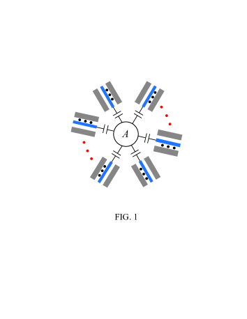
Figure 1: (Color online) Diagram of a coupler qubit $A$ (circle at the center) and $N$ cavities ($1,2,...,N$) each hosting qubits. Each cavity here is a one-dimensional coplanar waveguide transmission line resonator. The circle $A$ represents a SC qubit, which is capacitively coupled to each cavity. A dark dot represents an intra-cavity SC qubit. For simplicity, only three qubits are drawn in each cavity.

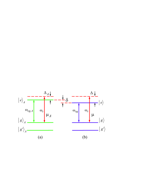
Figure 2: (Color online) (a) Each cavity is dispersively coupled to the $\left|g\right\rangle\leftrightarrow\left|e\right\rangle$ transition of the coupler qubit $A$, with coupling strength $\mu_{A}$ and detuning $\Delta_{A}=\omega_{c}-\omega_{eg,A}$. Here, $\omega_{c}$ is the cavity frequency while $\omega_{eg,A}$ is the $\left|g\right\rangle\leftrightarrow\left|e\right\rangle$ transition frequency of the coupler qubit $A$. (b) Each cavity is dispersively coupled to its hosting intra-cavity qubits’ $\left|g\right\rangle\leftrightarrow\left|e\right\rangle$ transition, with coupling strength $\mu$ and detuning $\Delta=\omega_{c}-\omega_{eg}$. Here, $\omega_{eg}$ is the $\left|g\right\rangle\leftrightarrow\left|e\right\rangle$ transition frequency of the intra-cavity qubits. In addition, $\delta=\Delta-\Delta_{A}$. In (a) and (b), a horizontal solid line represents an energy level of a qubit; and each vertical (red) double-arrow line, linked to a middle solid line and a top (red) dashed line, represents the cavity frequency $\omega_{c}$. For simplicity, we here consider the case when the level spacing between the two lowest levels is smaller than that between the upper two levels. This type of level structure is available in superconducting charge qubits or flux qubits. Alternatively, the level spacing between the two lowest levels can be larger than that between the upper two levels, which applies to superconducting phase, transmon or Xmon qubits. In (a) and (b), the ground level is labeled by $\left|g^{\prime}_{A}\right\rangle$ ($\left|g^{\prime}\right\rangle$) and the first excited level is denoted as $\left|g_{A}\right\rangle$ ($\left|g\right\rangle$). One could also denote the ground level as $\left|g_{A}\right\rangle$ ($\left|g\right\rangle$) and the first excited level as $\left|g^{\prime}_{A}\right\rangle$ ($\left|g^{\prime}\right\rangle$).

We consider a system composed of $N$ cavities and assume that cavity $j$ hosts $m_{j}$ SC qubits denoted as $j_{1},$ $j_{2},...,$ and $j_{m_{j}}$. These cavities ($1,2,...,N$) are coupled to a common SC qubit $A$ (coupler qubit), as shown in Fig. 1. Each qubit considered here has three levels, which are denoted as $\left|g\right\rangle,$ $\left|g^{\prime}\right\rangle,$ and $\left|e\right\rangle$ (Fig. 2). The two logical states of each intra-cavity qubit are represented by the two levels $\left|g\right\rangle$ and $\left|g^{\prime}\right\rangle$, while those of the coupler qubit are represented by the two levels $\left|g^{\prime}\right\rangle$ and $\left|e\right\rangle.$ The third level $\left|e\right\rangle$ for each intra-cavity qubit or $\left|g\right\rangle$ for the coupler qubit acts as an auxiliary level for realizing, e.g., a conditional phase shift. The level spacing of the coupler qubit $A$ is different from those of the intra-cavity qubits. The $\left|g\right\rangle\leftrightarrow\left|e\right\rangle$ transition of the intra-cavity qubits is coupled to their respective cavities with coupling strength $\mu,$ while the $\left|g\right\rangle\leftrightarrow\left|e\right\rangle$ transition of the coupler qubit $A$ is coupled to all the cavities with coupling strength $\mu_{A}$ (Fig. 2). We here assume that the level $\left|g^{\prime}\right\rangle$ of each qubit is not affected during the operation, which can be a good approximation when the transitions between $\left|g^{\prime}\right\rangle$ and other levels are sufficiently weak or the relevant transition frequencies are highly detuned from the cavity frequency. The level spacings of superconducting qubits can be rapidly adjusted by varying the external control parameters (e.g., the magnetic flux applied to a superconducting loop for phase, transmon or flux qubits; see e.g. [20,71-73]), so that the transitions associated with $\left|g^{\prime}\right\rangle$ can be tuned far off-resonance with the resonators. In the interaction picture with respect to the free Hamiltonian of the system (not shown for simplicity), the Hamiltonian is given by

$$H=\sum_{j=1}^{N}\mu\left(e^{-i\Delta t}a_{j}J_{j}^{+}+e^{i\Delta t}a_{j}^{\dagger}J_{j}\right)+\sum_{j=1}^{N}\mu_{A}\left(e^{-i\Delta_{A}t}a_{j}\sigma_{A}^{+}+e^{i\Delta_{A}t}a_{j}^{\dagger}\sigma_{A}\right),$$ (1)

where $J_{j}^{+}=\sum_{i=1}^{m_{j}}\sigma_{j_{i}}^{+},$ $J_{j}=\sum_{i=1}^{m_{j}}\sigma_{j_{i}},$ $\sigma_{j_{i}}^{+}=\left|e\right\rangle_{j_{i}}\left\langle g\right|,$ $\sigma_{j_{i}}=\left|g\right\rangle_{j_{i}}\left\langle e\right|,\sigma_{A}^{+}=\left|e\right\rangle_{A}\left\langle g\right|,$ $\sigma_{A}=\left|g\right\rangle_{A}\left\langle e\right|,$ $\Delta=\omega_{c}-\omega_{eg},$ and $\Delta_{A}=\omega_{c}-\omega_{eg,A}.$ Here, $\omega_{c}$ is the cavity frequency; and $\omega_{eg}$ and $\omega_{eg,A}$ are the $\left|g\right\rangle\leftrightarrow\left|e\right\rangle$ transition frequencies for the intra-cavity qubits and the coupler qubit $A$, respectively (Fig. 2).

Under the large-detuning condition $\Delta,\Delta_{A},\gg\mu,\mu_{A}$, $\left|\delta\right|=\left|\Delta-\Delta_{A}\right|,$ the dynamics governed by $H$ is equivalent to that decided by the following effective Hamiltonian [74-76]

$$H_{\mathrm{eff}} = \frac{\mu^{2}}{\Delta}\sum_{j=1}^{N}\left({G}_{j}a_{j}^{+}a_{j}-E_{j}a_{j}a_{j}^{+}\right)$$ (2)

$$\ \ +\frac{\mu_{A}^{2}}{\Delta_{A}}\sum_{j=1}^{N}\left({G}_{A}a_{j}^{+}a_{j}-E_{A}a_{j}a_{j}^{+}\right)$$

$$\ \ -\frac{\mu^{2}}{\Delta}\sum_{j=1}^{N}\left(J_{j}J_{j}^{+}-{G}_{j}\right)$$

$$\ \ -\lambda\sum_{j=1}^{N}(e^{-i\delta t}J_{j}\sigma_{A}^{+}+H.c.)$$

$$\ \ +\sum_{j\neq k=1}^{N}\lambda_{jk}\left(a_{j}a_{k}^{+}+H.c.\right)\left(E_{A}-G_{A}\right),$$

where $\delta=\Delta-\Delta_{A},$ ${G}_{j}=\sum_{i=1}^{m_{j}}\left|g\right\rangle_{j_{i}}\left\langle g\right|,$ ${E}_{j}=\sum_{i=1}^{m_{j}}\left|e\right\rangle_{j_{i}}\left\langle e\right|,$ ${G}_{A}=\left|g\right\rangle_{A}\left\langle g\right|,$ ${E}_{A}=\left|e\right\rangle_{A}\left\langle e\right|,$ $\lambda_{jk}=\mu_{A}^{2}/\Delta_{A},$ and $\lambda=\frac{\mu\mu_{A}}{2}\left(\frac{1}{\Delta}+\frac{1}{\Delta_{A}}\right).$ The terms in the first and second lines of (2) account for the ac-Stark shifts of the level $\left|g\right\rangle$ ($\left|e\right\rangle$) of the intra-cavity qubits and the coupler qubit $A$ induced by the corresponding cavity modes, respectively. In addition, the terms in the third line describe the effective dipole-dipole interaction between the intra-cavity qubits located in the same cavities. The terms in the fourth line describe the dipole-dipole interaction between the intra-cavity qubits and the coupler qubit $A$, and the terms in the last (fifth) line characterize the coupling between any two cavities.

If each cavity is initially in a vacuum state, the Hamiltonian (2) reduces to 

$$H_{\mathrm{eff}} = -\frac{\mu^{2}}{\Delta}\sum_{j=1}^{N}E_{j}-\frac{N\mu_{A}^{2}}{\Delta_{A}}E_{A}$$ (3)

$$\ \ -\frac{\mu^{2}}{\Delta}\sum_{j=1}^{N}\left(J_{j}J_{j}^{+}-{G}_{j}\right)$$

$$\ \ -\lambda\sum_{j=1}^{N}(e^{-i\delta t}J_{j}\sigma_{A}^{+}+H.c.).$$

According to [74], if $\left|\delta\right|\gg\lambda,$ $\frac{N\mu^{2}}{\Delta}$, $\frac{N\mu_{A}^{2}}{\Delta_{A}}$, the terms in the last line can be replaced by $\frac{\lambda^{2}}{\delta}[\sum_{j=1}^{N}J_{j}\sigma_{A}^{+},\sum_{j=1}^{N}J_{j}^{+}\sigma_{A}]$. Thus, the dynamics governed by Hamiltonian (3) is approximately equivalent to that by the following Hamiltonian 

$$H_{\mathrm{eff}}^{{}^{\prime}} = -\frac{\mu^{2}}{\Delta}\sum_{j=1}^{N}E_{j}-\frac{N\mu_{A}^{2}}{\Delta_{A}}E_{A}$$ (4)

$$\ \ -\frac{\mu^{2}}{\Delta}\sum_{j=1}^{N}\left(J_{j}J_{j}^{+}-{G}_{j}\right)$$

$$\ \ +\frac{\lambda^{2}}{\delta}E_{A}\sum_{j=1}^{N}J_{j}\sum_{l=1}^{N}J_{l}^{+}-\frac{\lambda^{2}}{\delta}G_{A}\sum_{j=1}^{N}J_{j}^{+}\sum_{l=1}^{N}J_{l},$$

which can be rewritten as 

$$H_{\mathrm{eff}}^{{}^{\prime}} = -\frac{\mu^{2}}{\Delta}\sum_{j=1}^{N}E_{j}-\frac{N\mu_{A}^{2}}{\Delta_{A}}E_{A}$$ (5)

$$\ \ -\frac{\mu^{2}}{\Delta}\sum_{j=1}^{N}\sum_{i\neq k=1}^{m_{j}}\sigma_{j_{i}}\sigma_{j_{k}}^{+}$$

$$\ \ +\frac{\lambda^{2}}{\delta}E_{A}\sum_{j=1}^{N}\sum_{l=1}^{N}\sum_{i=1}^{m_{j}}\sum_{k=1}^{m_{l}}\sigma_{j_{i}}\sigma_{l_{k}}^{+}$$

$$\ \ -\frac{\lambda^{2}}{\delta}G_{A}\sum_{j=1}^{N}\sum_{l=1}^{N}\sum_{i=1}^{m_{j}}\sum_{k=1}^{m_{l}}\sigma_{j_{i}}^{+}\sigma_{l_{k}}.$$

When the level $\left|g\right\rangle$ of the coupler qubit and the level $\left|e\right\rangle$ of the intra-cavity qubits are not populated, the Hamiltonian (5) reduces to

$$H_{\mathrm{eff}}^{{}^{\prime}} = -\frac{N\mu_{A}^{2}}{\Delta_{A}}E_{A}+\frac{\lambda^{2}}{\delta}E_{A}\sum_{j=1}^{N}{G}_{j}$$

$$= -\frac{N\mu_{A}^{2}}{\Delta_{A}}\left|e\right\rangle_{A}\left\langle e\right|+\frac{\lambda^{2}}{\delta}\left|e\right\rangle_{A}\left\langle e\right|\otimes\sum_{j=1}^{N}\sum_{i=1}^{m_{j}}\left|g\right\rangle_{j_{i}}\left\langle g\right|.$$ (6)

This effective Hamiltonian can be turned off by tuning the qubit levels in such a way that the transitions between these levels are highly off-resonant with the cavities, and hence the qubits are effectively decoupled from the corresponding cavities.

III Entangling intra-cavity qubits and the coupler qubit

Let us go back to the setup in Fig. 1. Initially, the qubit system is decoupled from the cavity system, and each cavity is in the vacuum state. Assume that each intra-cavity SC qubit is in the state $\left|+\right\rangle=1/\sqrt{2}\left(\left|g^{\prime}\right\rangle+\left|g\right\rangle\right)$ and the coupler SC qubit is in the state $\alpha\left|g^{\prime}\right\rangle_{A}+\beta\left|e\right\rangle_{A}$ ($\left|\alpha\right|^{2}+\left|\beta\right|^{2}=1$). These states can be prepared from the qubit ground state with classical pulses. For simplicity, let us consider the case of $\left|g\right\rangle$ being the ground state (a case applied to the flux qubits considered in Sec. 5, with three levels illustrated in Fig. 6). The state $\left|g\right\rangle$ can be transformed to $\left|+\right\rangle$ by applying a $\pi/2$ pulse tuned to the $\left|g\right\rangle\leftrightarrow\left|g^{{}^{\prime}}\right\rangle$ transition [29]. The preparation of the state $\alpha\left|g^{\prime}\right\rangle_{A}+\beta\left|e\right\rangle_{A}$ consists of two steps: (i) apply a $\pi$ pulse, tuned to the $\left|g\right\rangle_{A}\leftrightarrow\left|e\right\rangle_{A}$ transition, to flip the state $\left|g\right\rangle_{A}$ to $\left|e\right\rangle_{A}$; (ii) employ a classical pulse to drive the $\left|g^{\prime}\right\rangle_{A}\leftrightarrow\left|e\right\rangle_{A}$ transition, with the Rabi frequency $\Omega$ and duration $t$ satisfying $\alpha=\cos\left(\Omega t\right)$ and $\beta=\sin\left(\Omega t\right).$

The initial state of the whole qubit system is thus given by

$$\left(\alpha\left|g^{\prime}\right\rangle_{A}+\beta\left|e\right\rangle_{A}\right)\otimes\prod_{j=1}^{N}\prod_{i=1}^{m_{j}}\left|+\right\rangle_{j_{i}}.$$ (7)

Now adjust the level spacings of qubits, so that the qubit-resonator coupling is turned on and the dynamics of the qubit system is governed by the effective Hamiltonian (6). One can see that under the Hamiltonian (6), the state (7) evolves into

$$\ \alpha\left|g^{\prime}\right\rangle_{A}\prod_{j=1}^{N}\prod_{i=1}^{m_{j}}\left|+\right\rangle_{j_{i}}+\beta e^{-iH_{\mathrm{eff}}^{\prime}t}\left|e\right\rangle_{A}\prod_{j=1}^{N}\prod_{i=1}^{m_{j}}\left|+\right\rangle_{j_{i}}$$

$$= \alpha\left|g^{\prime}\right\rangle_{A}\prod_{j=1}^{N}\prod_{i=1}^{m_{j}}\left|+\right\rangle_{j_{i}}$$ (8)

$$+\beta\exp\left(iN\mu_{A}^{2}t/\Delta_{A}\right)\left|e\right\rangle_{A}\prod_{j=1}^{N}\prod_{i=1}^{m_{j}}\left[\left|g^{\prime}\right\rangle_{j_{i}}+\exp\left(-i\lambda^{2}t/\delta\right)\left|g\right\rangle_{j_{i}}\right],$$

where we have used $H_{\mathrm{eff}}^{\prime}\left|g^{\prime}\right\rangle=0.$ Setting

$$\frac{N\mu_{A}^{2}}{\Delta_{A}}t = 2m\pi,$$ (9)

$$\frac{\lambda^{2}}{\left|\delta\right|}t = \pi,$$ (10)

where $m$ is an integer, Eq. (8) can be expressed as

$$\left|\mathrm{GHZ}\right\rangle=\alpha\left|g^{\prime}\right\rangle_{A}\prod_{j=1}^{N}\prod_{i=1}^{m_{j}}\left|+\right\rangle_{j_{i}}+\beta\left|e\right\rangle_{A}\prod_{j=1}^{N}\prod_{i=1}^{m_{j}}\left|-\right\rangle_{j_{i}},$$ (11)

where $\left|-\right\rangle=1/\sqrt{2}\left(\left|g^{\prime}\right\rangle-\left|g\right\rangle\right)$. Since $\left|-\right\rangle$ is orthogonal to $\left|+\right\rangle$, the state (11) is a multi-particle GHZ entangled state for the coupler qubit and the qubits distributed in multiple cavities. One can see that the entangled state preparation here is based on a $\pi$-phase shift on the state $\left|g\right\rangle$ of each intracavity qubit conditional upon the coupler qubit being in the state $\left|e\right\rangle_{A}.$ Note that by applying a classical pulse to the coupler qubit, the states $\left|g^{\prime}\right\rangle_{A}$ and $\left|e\right\rangle_{A}$ can be easily converted into the states $\left|+\right\rangle_{A}$ and $\left|-\right\rangle_{A}$, respectively. The operation sequence for preparing the GHZ state (11) is illustrated in Fig. 3.

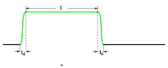
Figure 3: (Color online) Sequence of operations on each qubit (from left to right). Here, $t$ satisfies Eqs.(9) and (10), which is the qubit-cavity interaction time required for producing the GHZ state; while $t_{d}$ (within 1–3 ns [77,78]) is the time required to adjust the qubit level spacings. Note that the level spacings of qubits are tuned simultaneously. For simplicity, here and in Figs. (4) and (5), we assume that the time needed for adjusting the level spacings is the same for both intra-cavity qubits and coupler qubit.

Note that when the coupling of qubits to the mode in a cavity is spatially dependent, then different intra-cavity qubits will acquire different conditional phases. The coupler qubit would acquire a single-qubit phase, when its coupling to the cavity mode is deviated from the preset value. To eliminate the effect of this phase, the interaction time should be adjusted so that this phase is equal to $2m\pi$, with $m$ being an integer.

It should be mentioned that, in order to maintain the initial states and the prepared GHZ states of the qubit system, the coupler qubit and the intra-cavity qubits should be decoupled from their respective cavities before/after the entanglement production, which requires the qubit-cavity coupling to be switchable. This requirement can be readily achieved, by prior adjustment of the level spacings of the qubits [21,71-73] or the frequencies of the cavities. We note that the rapid tuning of microwave cavity frequencies has been experimentally demonstrated (e.g., in less than a few nanoseconds for a superconducting transmission line resonator [77,78]).

By preparing the initial state of the coupler qubit $A$ with different values of $\alpha$ and $\beta,$ the degree of entanglement for the GHZ state (11) can be adjusted and thus this protocol can be used to generate GHZ entangled states with an arbitrary degree of entanglement. As shown above, during the entanglement preparation no photons are excited in each cavity, no measurement is needed, and only a single-step operation is required.

IV Entangling intra-cavity qubits

In this section, we will briefly introduce two methods for preparing all intra-cavity SC qubits in a GHZ state. The first method requires a measurement on the coupler SC qubit, while the second one does not need any measurement.

A. Method 1

All qubits including the coupler qubit are first prepared in the GHZ state (11). One can see from Eq. (11) that through a unitary tranformation $\left|g^{\prime}\right\rangle_{A}\rightarrow\left(\left|g^{\prime}\right\rangle_{A}+\left|e\right\rangle_{A}\right)/\sqrt{2}$ and $\left|e\right\rangle_{A}\rightarrow\left(\left|g^{\prime}\right\rangle_{A}-\left|e\right\rangle_{A}\right)/\sqrt{2}$ and then a measurement on the coupler qubit $A$, the intra-cavity qubits will be prepared in one of the two GHZ states $\left|\mathrm{GHZ}\right\rangle^{\pm}=\alpha\prod_{j=1}^{N}\prod_{i=1}^{m_{j}}\left|+\right\rangle_{j_{i}}\pm\beta\prod_{j=1}^{N}\prod_{i=1}^{m_{j}}\left|-\right\rangle_{j_{i}}$ (depending on the measurement outcome). The operation sequence for preparing the states $\left|\mathrm{GHZ}\right\rangle^{\pm}$ is illustrated in Fig. 4.

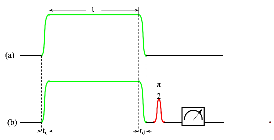
Figure 4: (Color online) (a) Sequence of operations on each intra-cavity qubit. (b) Sequence of operations on the coupler qubit. The green curves in (a) and (b) correspond to the operation for producing the GHZ state (11). In (b), the $\pi/2$ pulse transforms the state $\left|g^{\prime}\right\rangle_{A}\rightarrow\left(\left|g^{\prime}\right\rangle_{A}+\left|e\right\rangle_{A}\right)/\sqrt{2}$ and the state $\left|e\right\rangle_{A}\rightarrow\left(\left|g^{\prime}\right\rangle_{A}-\left|e\right\rangle_{A}\right)/\sqrt{2}$, and the square box with a meter represents a measurement on the coupler qubit along the basis $\{\left|g^{\prime}\right\rangle_{A}$, $\left|e\right\rangle_{A}\}$. Note that the operations in (a) and (b) are performed from left to right.

The two GHZ states $\left|\mathrm{GHZ}\right\rangle^{+}$ and $\left|\mathrm{GHZ}\right\rangle^{-}$ can be converted into each other through the local operation on any one of intra-cavity qubits (say qubit $j_{1}$): $\left|-\right\rangle_{j_{1}}\rightarrow-\left|-\right\rangle_{j_{1}}$ and $\left|+\right\rangle_{j_{1}}\rightarrow\left|+\right\rangle_{j_{1}}$. In this sense, the intra-cavity qubits can be prepared in a GHZ entangled state deterministically.

As discussed here, a measurement on the coupler qubit is necessary to prepare the intra-cavity qubits in a GHZ state. Note that fast and highly accurate measurements on the state of a SC qubit are experimentally available at this time (e.g., see [14]). In the following, we will propose an alternative approach for entangling the intra-cavity qubits, which does not require any measurement.

B. Method 2

Assume that one intra-cavity SC qubit, say qubit 1₁ in cavity 1, is initially in the state $\left|g^{\prime}\right\rangle,$ each of all remaining intra-cavity SC qubits is initially in the state $\left|+\right\rangle,$ and the coupler SC qubit $A$ is in the state $\alpha\left|g^{\prime}\right\rangle_{A}+\beta\left|e\right\rangle_{A}$. Then the initial state of the whole system is thus given by

$$\left|\mathrm{initial}\right\rangle=\left|g^{\prime}\right\rangle_{1_{1}}\prod_{i=2}^{m_{1}}\left|+\right\rangle_{1_{i}}\otimes\prod_{j=2}^{N}\prod_{i=1}^{m_{j}}\left|+\right\rangle_{j_{i}}\otimes\left(\alpha\left|g^{\prime}\right\rangle_{A}+\beta\left|e\right\rangle_{A}\right).$$ (12)

The procedure for preparing intra-cavity qubits in a GHZ entangled state is listed as follows:

Step 1: Keep qubit $1_{1}$ decoupled from cavity $1,$ while adjust the level spacings of other qubits such that their dynamics is governed by the Hamiltonian (6) (not including qubit $1_{1}$) for an interaction time $t$ satisfying Eqs. (9) and (10). By a similar derivation as shown in Eq. (8), one can easily find that the state (12) changes to

$$\left|g^{\prime}\right\rangle_{1_{1}}\left(\alpha\prod_{i=2}^{m_{1}}\left|+\right\rangle_{1_{i}}\otimes\prod_{j=2}^{N}\prod_{i=1}^{m_{j}}\left|+\right\rangle_{j_{i}}\otimes\left|g^{\prime}\right\rangle_{A}+\beta\prod_{i=2}^{m_{1}}\left|-\right\rangle_{1_{i}}\otimes\prod_{j=2}^{N}\prod_{i=1}^{m_{j}}\left|-\right\rangle_{j_{i}}\otimes\left|e\right\rangle_{A}\right).$$

Then, adjust the level spacings of the qubits such that the qubit system is decoupled from the cavities.

Step 2: Perform the operations, $\left|g^{\prime}\right\rangle_{1_{1}}\rightarrow\left|g\right\rangle_{1_{1}}$ and $\left|g^{\prime}\right\rangle_{A}\rightarrow\left|g\right\rangle_{A},$ by applying classical pulses to qubit $1_{1}$ and the coupler qubit. In addition, perform a swap operation $\left|g\right\rangle_{1_{1}}\left|e\right\rangle_{A}\rightarrow-i\left|e\right\rangle_{1_{1}}\left|g\right\rangle_{A}$ [75], which can be achieved by adjusting the level spacings of qubit $1_{1}$ and the coupler qubit, such that the transitions $\left|g\right\rangle\rightarrow\left|e\right\rangle$ of qubits $1_{1}$ and the coupler qubit are dispersively coupled to cavity $1$ with the same detuning. Then the state (13) becomes

$$\left|\textrm{GHZ}\right\rangle\left|g\right\rangle_{A} = \left(\alpha\left|g\right\rangle_{1_{1}}\prod_{i=2}^{m_{1}}\left|+\right\rangle_{1_{i}}\otimes\prod_{j=2}^{N}\prod_{i=1}^{m_{j}}\left|+\right\rangle_{j_{i}}-i\beta\left|e\right\rangle_{1_{1}}\prod_{i=2}^{m_{1}}\left|-\right\rangle_{1_{i}}\otimes\prod_{j=2}^{N}\prod_{i=1}^{m_{j}}\left|-\right\rangle_{j_{i}}\right)\left|g\right\rangle_{A},$$

which shows that all intra-cavity qubits are deterministically prepared in a GHZ entangled state and disentangled from the coupler qubit. Since no measurement is involved, the operations above are unitary. The operation sequence for preparing the GHZ state is illustrated in Fig. 5.

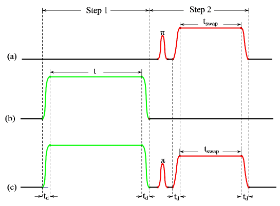
Figure 5: (Color online) (a) Sequence of operations on qubit $1_{1}$. (b) Sequence of operations on the intra-cavity qubits (except for qubit $1_{1}$). (c) Sequence of operations on the coupler qubit $A$. The green curves in (b) and (c) correspond to the operation described by step 1, which is for preparing the state (13). The red curves in (a) and (c) correspond to the operation of step 2 for preparing the state (14). The $\pi$ pulse in (a) transforms the state $\left|g^{\prime}\right\rangle_{1_{1}}\rightarrow\left|g\right\rangle_{1_{1}}$, while the $\pi$ pulse in (c) transforms the state $\left|g^{\prime}\right\rangle_{A}\rightarrow\left|g\right\rangle_{A}$. The right-hand square curves in (a) and (c) represent a swap operation described by $\left|g\right\rangle_{1_{1}}\left|e\right\rangle_{A}\rightarrow-i\left|e\right\rangle_{1_{1}}\left|g\right\rangle_{A}$ [75]. In (a) and (c), $t_{\mathrm{swap}}$ is the swap operation time. Note that the operations in (a), (b), and (c) are performed from left to right.

From the description given above, one can see that the entanglement production does not employ cavity photons. In addition, the GHZ state preparation here does not depend on the number of intra-cavity qubits, which requires only a few basic operations. Hence, the methods presented here for entangling the intra-cavity qubits are quite simple.

V Experimental feasibility of entangling multiple qubits: an example

To illustrate the experimental feasibility of our scheme, we consider a system of two cavites (i.e., two one-dimensional transmission line resonators) each hosting $M$ superconducting flux qubits (with $M\leqslant 4$) and coupled by a superconducting flux qubit $A.$ Figure 6 shows the setup for each cavity hosting four flux qubits. The three levels $\left|g\right\rangle,$ $\left|g^{\prime}\right\rangle,$ and $\left|e\right\rangle$ of each flux qubit are depicted in Fig. 7. The $\left|g\right\rangle\leftrightarrow\left|g^{\prime}\right\rangle$ transition of each flux qubit can be made weak by increasing the potential barrier and thus its coupling with the cavities is negligible. In reality, the $\left|g^{\prime}\right\rangle\leftrightarrow\left|e\right\rangle$ transition needs to be considered because the coupling between this transition and each cavity may turn out to affect the operation fidelity. Note that the $\left|g^{\prime}\right\rangle\leftrightarrow\left|e\right\rangle$ transition is much weaker than the $\left|g\right\rangle\leftrightarrow\left|e\right\rangle$ transition due to the potential barrier between the two wells.

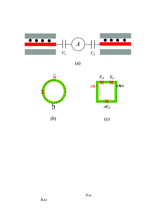
Figure 6: (Color online) (a) Setup of two one-dimensional transmission line resonators each hosting four flux qubits (dark dots) and coupled to flux qubit $A$ (in the middle circle). The coupler qubit $A$ is connected to the two resonators via capacitors $C_{1}$ and $C_{2}$, respectively. Each qubit could be a radio-frequency superconducting quantum interference device (rf SQUID) consisting of one Josephson junction enclosed by a superconducting loop as depicted in (b), or a superconducting device with three Josephson junctions enclosed by a superconducting loop as shown in (c). $E_{J}$ is the Josephson junction energy ($0.6<\alpha<0.8$). The superconducting loop of each qubit, which is a large circle for (b) while a large square for (c), is located in the plane of the resonators between the two lateral ground planes. Each intra-cavity qubit is coupled to its cavity via the magnetic flux through the superconducting loop of each qubit, which is created by the cavity magnetic field threading the superconducting loop. The intra-cavity qubits are placed at locations where the cavity magnetic fields are the same to achieve an identical coupling strength for each qubit. For each qubit, a tunable-coupler dc current line, e.g., the red dashed line in (b) or (c) placed on the qubit loop, creates a dc magnetic pulse threading the loop of each qubit, which is used for tuning the qubit level spacings. Note that the qubit level spacings can be tuned by varying the magnitude of the dc magnetic pulse through changing the current intensity. In addition, for each qubit, a microwave bias ac current line, e.g., the dark dashed line in (b) or (c) on the qubit loop, creates an ac magnetic pulse threading the loop of each qubit, which is used to prepare the initial state of each qubit or/and manipulate the state of each qubit during the GHZ state preparation.

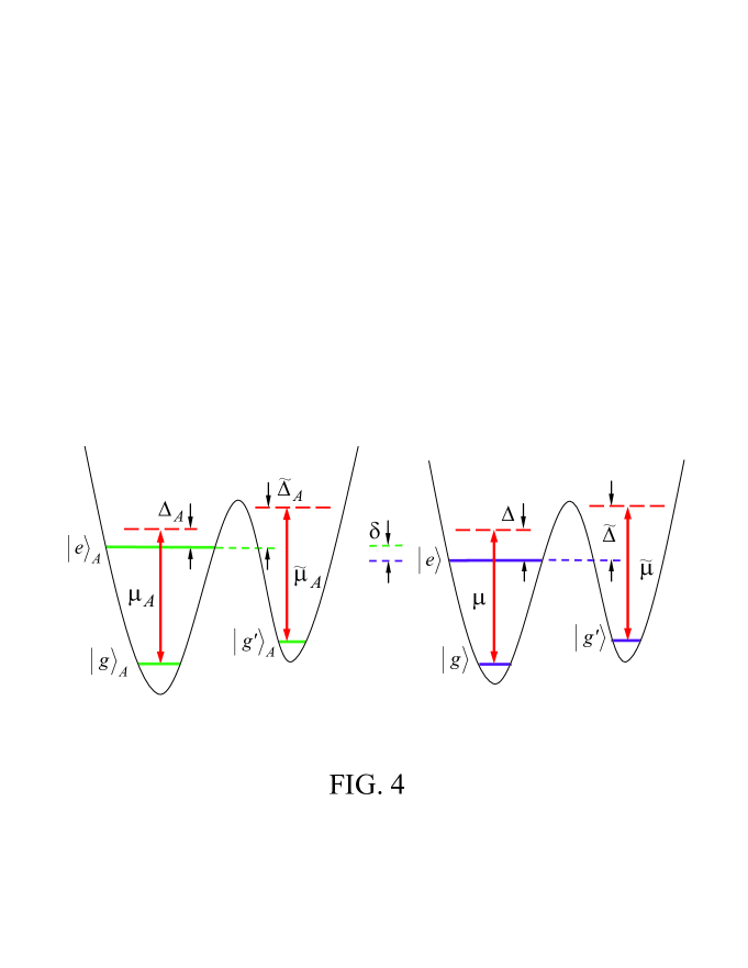
Figure 7: (Color online) Illustration of the qubit-cavity dispersive interaction. The left is for the coupler flux qubit $A$ , while the right is for the intra-cavity flux qubits. The tunneling between the two lowest levels is made weak by increasing the potential barrier, such that the level $\left|g^{\prime}\right\rangle$ can be stored for a long time.

When the unwanted coupling of the $\left|g^{\prime}\right\rangle\leftrightarrow\left|e\right\rangle$ transition with the cavities and the unwanted inter-cavity crosstalk are included, the Hamiltonian (1) is modified as

$$\widetilde{H} = \sum_{j=1}^{2}\mu\left(e^{-i\Delta t}a_{j}J_{j}^{+}+\mathrm{H.c.}\right)+\sum_{j=1}^{2}\mu_{A}\left(e^{-i\Delta_{A}t}a_{j}\sigma_{A}^{+}+\mathrm{H.c.}\right)$$ (15)

$$+\sum_{j=1}^{2}\widetilde{\mu}\left(e^{-i\widetilde{\Delta}t}a_{j}\widetilde{J}_{j}^{+}+\mathrm{H.c.}\right)+\sum_{j=1}^{2}\widetilde{\mu}_{A}\left(e^{-i\widetilde{\Delta}_{A}t}a_{j}\widetilde{\sigma}_{A}^{+}+\mathrm{H.c.}\right)$$

$$+\mu_{12}\left(a_{1}a_{2}^{+}+\mathrm{H.c.}\right),$$

where $J_{j}^{+}=\sum_{j=1}^{2}\sum_{i=1}^{M}\sigma_{j_{i}}^{+},$ $\widetilde{J}_{j}^{+}=\sum_{j=1}^{2}\sum_{i=1}^{M}\widetilde{\sigma}_{j_{i}}^{+},$ $\widetilde{\sigma}_{j_{i}}^{+}=\left|e\right\rangle_{j_{i}}\left\langle g^{\prime}\right|,$ and $\widetilde{\sigma}_{A}^{+}=\left|e\right\rangle_{A}\left\langle g^{\prime}\right|.$ The terms in the first (second) pair of parentheses in the second line describe the unwanted coupling between the $\left|g^{\prime}\right\rangle\leftrightarrow\left|e\right\rangle$ transition of intra-cavity qubits (coupler qubit) and the respective cavities with coupling strength $\widetilde{\mu}$ ($\widetilde{\mu}_{A}$) and detuning $\widetilde{\Delta}=\omega_{c}-\omega_{eg^{\prime}}$ ($\widetilde{\Delta}_{A}=\omega_{c}-\omega_{eg^{\prime},A}$). The terms in the last pair of parentheses describe the inter-cavity crosstalk between two cavities, with the inter-cavity coupling constant $\mu_{12}$.

The dynamics of the lossy system, with finite qubit relaxation, dephasing and photon lifetime being included, is determined by the following master equation

$$\frac{d\rho}{dt}=-i\left[\widetilde{H},\rho\right]+\sum_{j=1}^{2}\kappa_{j}\mathcal{L}\left[a_{j}\right]+P+Q,$$ (16)

with

$$P = \sum_{j=1}^{2}\sum_{i=1}^{M}\left\{\gamma_{{}_{eg}}\mathcal{L}\left[\sigma_{j_{i}}\right]+\gamma_{eg^{\prime}}\mathcal{L}\left[\widetilde{\sigma}_{j_{i}}\right]+\gamma_{g^{\prime}g}\mathcal{L}\left[\overline{\sigma}_{j_{i}}\right]\right\}$$ (17)

$$\ +\sum_{j=1}^{2}\sum_{i=1}^{M}\left\{\gamma_{e,\varphi}\left(E_{j_{i}}\rho E_{j_{i}}-E_{j_{i}}\rho/2-\rho E_{j_{i}}/2\right)\right\}$$

$$\ +\sum_{j=1}^{2}\sum_{i=1}^{M}\left\{\gamma_{g^{\prime},\varphi}\left(G_{j_{i}}^{\prime}\rho G_{j_{i}}^{\prime}-G_{j_{i}}^{\prime}\rho/2-\rho G_{j_{i}}^{\prime}/2\right)\right\},$$

$$Q = \gamma_{{}_{eg},A}\mathcal{L}\left[\sigma_{A}^{-}\right]+\gamma_{eg^{\prime},A}\mathcal{L}\left[\widetilde{\sigma}_{A}^{-}\right]+\gamma_{g^{\prime}g,A}\mathcal{L}\left[\overline{\sigma}_{A}^{-}\right]$$ (18)

$$\ +\gamma_{e,\varphi,A}\left(E_{A}\rho E_{A}-E_{A}\rho/2-\rho E_{A}/2\right)$$

$$\ +\gamma_{g^{\prime},\varphi,A}\left(G_{A}^{\prime}\rho G_{A}^{\prime}-G_{A}^{\prime}\rho/2-\rho G_{A}^{\prime}/2\right),$$

where $\overline{\sigma}_{j_{i}}=\left|g\right\rangle_{j_{i}}\left\langle g^{\prime}\right|,\overline{\sigma}_{A}=\left|g\right\rangle_{A}\left\langle g^{\prime}\right|;$ $E_{j_{i}}=\left|e\right\rangle_{j_{i}}\left\langle e\right|,G_{j_{i}}^{\prime}=\left|g^{\prime}\right\rangle_{j_{i}}\left\langle g^{\prime}\right|,G_{A}^{\prime}=\left|g^{\prime}\right\rangle_{A}\left\langle g^{\prime}\right|;$ and $\mathcal{L}\left[\Lambda\right]=\Lambda\rho\Lambda^{+}-\Lambda^{+}\Lambda\rho/2-\rho\Lambda^{+}\Lambda/2,$ with $\Lambda=a_{j},\sigma_{j_{i}},\widetilde{\sigma}_{j_{i}},\overline{\sigma}_{j_{i}},\sigma_{A},\widetilde{\sigma}_{A},\overline{\sigma}_{A}.$ Here, $\kappa_{j}$ is the photon decay rate of cavity $a_{j}$. In addition, $\gamma_{g^{\prime}g}$ is the energy relaxation rate of the level $\left|g^{\prime}\right\rangle$ of qubits, $\gamma_{eg}$ ($\gamma_{eg^{\prime}}$) is the energy relaxation rate of the level $\left|e\right\rangle$ of intra-cavity qubits for the decay path $\left|e\right\rangle\rightarrow\left|g\right\rangle$ ($\left|g^{\prime}\right\rangle$), and $\gamma_{e,\varphi}$ ($\gamma_{g^{\prime},\varphi}$) is the dephasing rate of the level $\left|e\right\rangle$ ($\left|g^{\prime}\right\rangle$) of intra-cavity qubits. The symbols $\gamma_{g^{\prime}g,A},$ $\gamma_{eg,A},$ $\gamma_{eg^{\prime},A},$ $\gamma_{e,\varphi,A},$ and $\gamma_{g^{\prime},\varphi,A}$ denote the corresponding decoherence rates of the coupler qubit $A.$

The fidelity of the operation is given by [79]

$$\mathcal{F}=\sqrt{\left\langle\psi_{\mathrm{id}}\right|\rho\left|\psi_{\mathrm{id}}\right\rangle},$$ (19)

where $\left|\psi_{\mathrm{id}}\right\rangle$ is the output state of an ideal system (i.e., without dissipation, dephasing, and crosstalks) as discussed in the previous section, and $\rho$ is the final density operator of the system when the operation is performed in a realistic physical system. Without loss of generality, consider now that the qubit system is initially in the state $\prod_{j=1}^{2}\prod_{i=1}^{M}\left|+\right\rangle_{j_{i}}\left(\left|g^{\prime}\right\rangle_{A}+\left|e\right\rangle_{A}\right)/\sqrt{2}$ (with $M\leq 4$), and the two cavities are initially in a vacuum state, for which the ideal state $\left|\psi_{\mathrm{id}}\right\rangle$ is the one given in Eq. (11) with $\alpha=\beta=1/\sqrt{2}$.

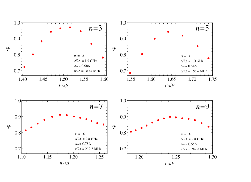
Figure 8: (Color online) Fidelity versus $\mu_{A}/\mu$. Here, $n$ is the total number of qubits including the coupler qubit. Also $n=3,5,7$ and $9$ correspond to the cases of each cavity hosting one, two, three and four qubits, respectively. To have an achievable good fidelity with reasonable parameters, we increase $\Delta/(2\pi)=2$ from 1 to 2 GHz, when going from 5 to 7 qubits. For $n=3,$ $5,$ $7$ and $9,$ a high fidelity $\sim 97.2\%,$ $94.3\%,$ $91.3\%,$ and $90.1\%$ can be achieved with $\mu_{A}/\mu$ being $1.516,$ $1.641,$ $1.174,$ and $1.242$, respectively.

We consider identical intra-cavity flux qubits. Given $\Delta,$ $\Delta_{A},$ and $m,$ the coupling constant $\mu$ is determined by $\mu=\sqrt{2N\left|\delta\right|\Delta_{A}/m}\Delta/\left(\Delta+\Delta_{A}\right)$ [derived from Eqs. (9) and (10)]. We set $\widetilde{\mu}=0.1\mu$ and $\widetilde{\mu}_{A}=0.1\mu_{A},$ which is a good approximation by increasing the potential barrier such that the transition matrix element between the two levels $\left|g^{\prime}\right\rangle$ and $\left|e\right\rangle$ is smaller than that between the two levels $\left|g\right\rangle$ and $\left|e\right\rangle$ by one order of magnitude (Fig. 7). We choose $\Delta/\left(2\pi\right)=1.0$ GHz for $n=3$ and $n=5$, while $\Delta/\left(2\pi\right)=2.0$ GHz for $n=7$ and $n=9$. Here, $n=2M+1$ is the total number of qubits including the coupler qubit. In addition, we set $\widetilde{\Delta}=\Delta+2\pi\times 1.5$ GHz and $\widetilde{\Delta}_{A}=\Delta_{A}+2\pi\times 1.5$ GHz. We now choose $\kappa_{j}^{-1}=15$ $\mu$s, $\gamma_{e,\varphi}^{-1}=5$ $\mu$s, $\gamma_{g^{\prime},\varphi}^{-1}=7.5$ $\mu$s, $\gamma_{eg}^{-1}=5$ $\mu$s, $\gamma_{eg^{\prime}}^{-1}=7.5$ $\mu$s, and $\gamma_{g^{\prime}g}^{-1}=15$ $\mu$s (a conservative consideration, e.g., see Ref. [9]). Our numerical calculations show that when $\mu_{12}$ is smaller than $\mu_{A}$ by two orders of magnitude, the effect of the inter-cavity crosstalk on the operation is negligible. Thus, we now set $\mu_{12}=0.01\mu_{A}.$ With the parameters chosen here and by numerically optimizing the parameters $m,$ $\mu,$ and $\Delta_{A}$, the fidelity versus $\mu_{A}/\mu$ is plotted in Fig. 8 for $n=3,$ $5,$ $7$ and $9.$ From Fig. 8, one can see that for $n=3,$ $5,$ $7$ and $9,$ a high fidelity $\sim 97.2\%,$ $94.3\%,$ $91.3\%,$ and $90.1\%$ can be achieved with the optimized values of $\mu_{A}/\mu$ being $1.516,$ $1.641,$ $1.174,$ and $1.242$, respectively. We remark that the fidelity can be further increased by improving the system parameters.

Figure 8 shows that with the parameter values chosen above the large detuning condition is not well satisfied for the optimized fidelity, e.g., $\Delta_{A}/\mu_{A}\sim 3.95$ for $n=9$, which implies that the state evolution determined by the effective Hamiltonian (6) can be a good approximation with a suitable choice of parameters, even when the qubit-cavity detunings are not much larger than the coupling strengths. This result has a quantitative explanation. Beyond the large detuning regime, when the coupler qubit is initially in the state $\left|e\right\rangle$, the total cavity-qubit system undergoes Rabi oscillations in the corresponding single-excitation subspace. The associated Rabi frequencies have a dependence on the number of the intracavity qubits in the state $\left|g\right\rangle$. With a suitable choice of the qubit-cavity coupling strengths and detunings, all of the state components with the coupler qubit being initially in $\left|e\right\rangle$ can return to their initial forms almost at the same time, with the resulting phase shift being related to the corresponding Rabi frequency.

As discussed in [39,80], the condition $\mu_{12}\leq 0.01\mu_{A}$ can be met with the typical capacitive cavity-qubit coupling. Figure 8 shows that at the optimum points, the coupling strengths are $\left\{\mu/2\pi,\mu_{A}/2\pi\right\}\sim\{180.4$ MHz, $273.5$ MHz$\}$ ($n=3$), $\{156.4$ MHz, $256.75$ MHz$\}$ ($n=5$), $\{232.7$ MHz, $273.2$ MHz$\}$ ($n=7$), and $\{269.0$ MHz, $334.0$ MHz$\}$ ($n=9$). The coupling strengths of these values are readily achievable in experiments because a coupling strength $\sim 636$ MHz has been reported for a superconducting flux device coupled to a one-dimensional transmission line resonator [26]. For a flux qubit, the $\left|g\right\rangle\leftrightarrow\left|e\right\rangle$ transition frequency could be between 5 GHz and 20 GHz. Thus, we can choose $\omega_{c}/2\pi\sim 7.5$ GHz. For the value of $\kappa_{j}^{-1}$ used in the numerical calculation, the required quality factor for each cavity is $Q=\kappa_{j}^{-1}\omega_{c}\sim 7.1\times 10^{5},$ which is available in experiments according to previous reports [81,82]. Therefore, the high-fidelity creation of GHZ states of up to nine qubits by using this proposal is feasible with current circuit QED technology.

Table 1: Qubits $1_{1}$, $1_{2}$, $1_{3}$, and $1_{4}$ are four qubits placed in one cavity; while Qubits $2_{1}$, $2_{2}$, $2_{3}$, and $2_{4}$ are four qubits placed in the other cavity. Here $\mu$ takes the same value used in Fig. 8.

Table 2: Here $\Delta$ takes the same value used in Fig. 8.

To see how well this method works in a more realistic situation, we now consider inhomogeneous coupling of qubits to the mode in each cavity, non-uniform distribution of qubit frequencies, imperfect preparation of the initial states, error in the operation time, and the existence of thermal photons in each cavity. The density operator of a thermal state of each cavity is described by $\rho=\sum\limits_{n=0}^{\infty}\frac{\overline{n}^{n}}{\left(1+\overline{n}\right)^{n+1}}\left|n\right\rangle\left\langle n\right|,$ with $\overline{n}$ being the average photon number and $\left|n\right\rangle$ being an $n$-photon state. In our numerical simulation, we choose $\overline{n}=0.1$. The initial state of the qubit system is modified as $\prod_{j=1}^{2}\prod_{i=1}^{M}\left(\sqrt{\frac{1+\varepsilon}{2}}\left|g^{\prime}\right\rangle_{j_{i}}+\sqrt{\frac{1-\varepsilon}{2}}\left|g\right\rangle_{j_{i}}\right)\left(\sqrt{\frac{1+\varepsilon}{2}}\left|g^{\prime}\right\rangle_{A}+\sqrt{\frac{1-\varepsilon}{2}}\left|e\right\rangle_{A}\right).$ For simplicity, we here consider the identical error $\varepsilon$ for the preparation of the initial state of each qubit. Without loss of generality, we will numerically investigate how the maximum fidelity in each subfigure of Fig. 8 is affected by the above-mentioned factors.

As mentioned above, the coupling constant $\mu_{A}$ of the coupler qubit, corresponding to the maximum fidelity in each subfigure of Fig. 8, is calculated to be $\mu_{A}=1.516\mu$ for $n=3$; $\mu_{A}=1.641\mu$ for $n=5$; $\mu_{A}=1.174\mu$ for $n=7$; and $\mu_{A}=1.242\mu$ for $n=9$. Here, the value of $\mu$ is shown in Fig. 8. In addition, the detuning $\Delta_{A}$ for the coupler qubit takes the same value as in Fig. 8.

The coupling constants and the detunings for the intra-cavity qubits are listed in Tables 1 and 2, where up to $1\%$ inhomogeneous coupling constants and up to $5\%$ non-uniform detunings are considered. In Tables 1 and 2, the values of $\mu$ and $\Delta$ are the same as those in Fig. 8.

With the parameters chosen above, in Fig. 9 we present a numerical simulation of the fidelity versus $t/T$ for $\varepsilon=0,$ $0.05,$ and $0.1.$ Here, $t$ is the operation time, while $T$ is the optimal operation time corresponding to the maximum fidelities in Fig. 8, which are 46.55 ns, 67.94 ns, 167.19 ns, 106.43 ns for $n=3,5,7,$ and $9$, respectively. From Fig. 9, one can see that the fidelity is insensitive to the error $\varepsilon$ but is significantly affected by the error in operation time. For $t=0.95T$ or $1.05T$ (i.e., $5\%$ operational time error), the fidelity drops down to $\lesssim 0.5.$ Note that for $t=T,$ good fidelities $\gtrsim 0.939$ for $n=3$, $\gtrsim 0.845$ for $n=5$, $\gtrsim 0.778$ for $n=7$, and $\gtrsim 0.760$ for $n=9$ can be obtained.

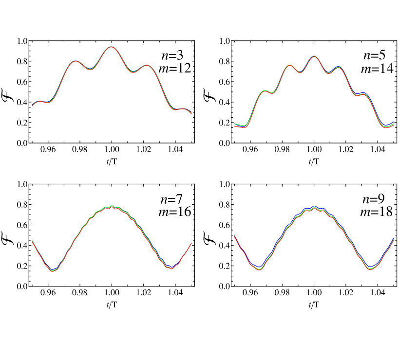
Figure 9: (Color online) Fidelity versus $t/T$. Here, $t$ is the operation time, while $T$ is the operation time corresponding to the maximum fidelities in Fig. 5, which are 46.55 ns, 67.94 ns, 167.19 ns, 106.43 ns for $n=3,5,7,$ and $9$, respectively. The blue, green, and red curves correspond to $\varepsilon=0,0.05$, and $0.1$. For $t=T$, the fidelities corresponding to $\varepsilon=\left\{0,0.05,0.1\right\}$ are: $\left\{0.942,0.941,0.939\right\}$ for $n=3$; $\left\{0.850,0.848,0.845\right\}$ for $n=5$; $\left\{0.790,0.789,0.778\right\}$ for $n=7$; and $\left\{0.786,0.769,0.760\right\}$ for $n=9$.

It is worthwhile to discuss the advantage of utilizing negative detunings versus positive detunings. For the flux qubits with three levels $\left|g\right\rangle$, $\left|g^{\prime}\right\rangle$, and $\left|e\right\rangle$ shown in Fig. 7, the purpose of using a negative detuning is to increase the detuning of the $\left|g^{\prime}\right\rangle\leftrightarrow\left|e\right\rangle$ transition frequency from the cavity frequency, in order to reduce the effect of this unwanted transition on the operation fidelity. It can be seen from Fig. 7 that the detuning of the $\left|g^{\prime}\right\rangle\leftrightarrow\left|e\right\rangle$ transition frequency from the cavity frequency would be smaller when using a positive detuning (i.e, the case when the cavity frequency is smaller than the $\left|g^{\prime}\right\rangle\leftrightarrow\left|e\right\rangle$ transition frequency), compared to using the negative detuning. 

VI Conclusion

We have proposed a general and efficient way to entangle SC qubits in a multi-cavity system. In principle, GHZ states of an arbitrary number of intra-caviy qubits plus the coupler qubit can be created through a single operation and without any measurements. Since only virtual photon processes take place, the decoherence caused by cavity decay and the effect of unwanted inter-cavity crosstalk are greatly suppressed. Also, the higher energy level is not occupied for any intra-cavity qubit; thus decoherence from the qubits is much reduced. In addition, we have introduced two simple methods for entangling the intra-cavity qubits in a GHZ state. Our numerical simulations show that it is feasible to generate high-fidelity GHZ entangled states with up to nine SC qubits in a circuit consisting of two resonators. We hope this will stimulate future experimental activities. The method presented here is quite general and can be applied to various other physical systems. We believe that the cluster-style architecture shown in Fig. 1 has applications in fault-tolerant code for scalable quantum computing. Multiple physical qubits in each cavity can be used to construct a logic qubit, as required by error-correction protocols. The system can also be used to simulate the dynamics of the star-type coupled spin system, where many spins are coupled to a common spin.

ACKNOWLEDGMENTS

We very gratefully acknowledge Dr. Anton Frisk Kockum for a critical reading of the manuscript. This work was partly supported by the RIKEN iTHES Project, the MURI Center for Dynamic Magneto-Optics via the AFOSR award number FA9550-14-1-0040, and a Grant-in-Aid for Scientific Research (A). It was also partially supported by the Major State Basic Research Development Program of China under Grant No. 2012CB921601, the National Natural Science Foundation of China under Grant Nos. [11074062, 11374083], the Zhejiang Natural Science Foundation under Grant No. LZ13A040002, the funds of Hangzhou Normal University under Grant Nos. [HSQK0081, PD13002004], and the funds of Hangzhou City for supporting the Hangzhou-City Quantum Information and Quantum Optics Innovation Research Team.

References

References

- (1) Buluta I, Ashhab S and Nori F 2011 Rep. Prog. Phys. 74 104401
- (2) Bylander J et al 2011 Nature Phys. 7 565
- (3) Paik H et al 2011 Phys. Rev. Lett. 107 240501
- (4) Chang J B et al 2013 Appl. Phys. Lett. 103 012602
- (5) Chow J K et al 2012 Phys. Rev. Lett. 109 060501
- (6) Barends R et al 2013 Phys. Rev. Lett. 111 080502
- (7) Chow J M et al 2014 Nature Comm. 5 4015
- (8) Chen Y et al 2014 Phys. Rev. Lett. 113 220502
- (9) Stern M, Catelani G, Kubo Y, Grezes C, Bienfait A, Vion D, Esteve D and Bertet P 2014 Phys. Rev. Lett. 113 123601
- (10) Filipp S et al 2009 Phys. Rev. Lett 102 200402
- (11) Bialczak R C et al 2010 Nature Phys. 6 409
- (12) Neeley M et al 2010 Nature 467 570
- (13) Yamamoto T et al 2010 Phys. Rev. B 82 184515
- (14) Reed M D et al 2010 Phys. Rev. Lett. 105 173601
- (15) Jeffrey E et al 2014 Phys. Rev. Lett. 112 190504
- (16) Liu Y X, Sun H C, Peng Z H, Miranowicz A, Tsai J S and Nori F 2014 Scientific Reports 4 7289
- (17) Yang C P, Chu S I and Han S 2003 Phys. Rev. A 67 042311
- (18) You J Q and Nori F 2003 Phys. Rev. B 68 064509
- (19) Blais A, Huang R S, Wallraff A, Girvin S M and Schoelkopf R J 2004 Phys. Rev. A 69 062320
- (20) You J Q and Nori F 2005 Phys. Today 58 42
- (21) Clarke J and Wilhelm F K 2008 Nature 453 1031
- (22) You J Q and Nori F 2011 Nature 474 589
- (23) Xiang Z L, Ashhab S, You J Q and Nori F 2013 Rev. Mod. Phys. 85 623
- (24) Majer J et al 2007 Nature 449 443
- (25) DiCarlo L et al 2009 Nature 460 240
- (26) Niemczyk T et al 2010 Nature Phys. 6 772
- (27) Blais A, Maassen van den Brink A and Zagoskin A M 2003 Phys. Rev. Lett. 90 127901
- (28) Plastina F and Falci G 2003 Phys. Rev. B 67 224514
- (29) Yang C P and Han S 2005 Phys. Rev. A 72 032311
- (30) Helmer F and Marquardt F 2009 Phys. Rev. A 79 052328
- (31) Bishop L S et al 2009 New J. Phys. 11 073040
- (32) Yang C P, Liu Y X and Nori F 2010 Phys. Rev. A 81 062323
- (33) Leek P J, Filipp S, Maurer P, Baur M, Bianchetti R, Fink J M, Goppl M, Steffen L and Wallraff A 2009 Phys. Rev. B 79 180511(R)
- (34) DiCarlo L et al 2010 Nature 467 574
- (35) Chow J M et al 2011 Phys. Rev. Lett. 107 080502
- (36) Mariantoni M et al 2011 Science 334 61
- (37) Fedorov A, Steffen L, Baur M, da Silva M P and Wallraff A 2012 Nature 481 170
- (38) Strauch F W, Jacobs K and Simmonds R W 2010 Phys. Rev. Lett. 105 050501
- (39) Yang C P, Su Q P and Han S 2012 Phys. Rev. A 86 022329
- (40) Yang C P, Su Q P, Zheng S B and Han S 2013 Phys. Rev. A 87 022320
- (41) Merkel S T and Wilhelm F K 2010 New J. Phys. 12 093036
- (42) Wang H et al 2011 Phys. Rev. Lett. 106 060401
- (43) Hua M, Tao M J and Deng F G 2014 Phys. Rev. A 90 012328
- (44) Matsuo S, Ashhab S, Fujii T, Nori F, Nagai K and Hatakenaka N 2006 Generation of Bell states and Greenberger-Horne-Zeilinger states in superconducting phase qubits, Quantum Communication, Measurement and Computing, (no. 8), O. Hirota, J. H. Shapiro, M. Sasaki, editors (NICT Press)
- (45) Yang C P, Su Q P and Nori F 2013 New J. Phys. 15 115003
- (46) Steffen L et al 2013 Nature 500 319
- (47) Greenberger D M, Horne M A and Zeilinger A 1989 In Bell Theorem, Quantum Theory and Conceptions of the Universe, edited by M. Kafatos (Kluwer Academic, Dordrecht)
- (48) Hillery M, Bužek V and Berthiaume A 1999 Phys. Rev. A 59 1829
- (49) See, for many references, Bose S, Vedral V and Knight P L 1998 Phys. Rev. A 57 822
- (50) Devitt S J, Munro W J and Nemoto K 2013 Rep. Prog. Phys. 76 076001
- (51) Giovannetti V, Lloyd S and Maccone L Science 306 1330 2004
- (52) Bollinger J J, Itano W M, Wineland D J and Heinzen D J 1996 Phys. Rev. A 54 R4649
- (53) Huang Y F, Liu B H, Peng L, Li Y H, Li L, Li C F and Guo G C 2011 Nat. Commun. 2 546
- (54) Yao X C, Wang T X, Xu P, Lu H, Pan G S, Bao X H, Peng C Z, Lu C Y, Chen Y A and Pan J W 2012 Nat. Photonics 6 225
- (55) Monz T, Schindler P, Barreiro J T, Chwalla M, Nigg D, Coish W A, Harlander M, Hänsel W, Hennrich M and Blatt R 2011 Phys. Rev. Lett. 106 130506
- (56) Barends R et al Nature 2014 508 500
- (57) Dogra S, Dorai K and Arvind 2015 Phys. Rev. A 91 022312
- (58) You J Q et al 2003 Phys. Rev. B 68 024510; Wei L F et al 2006 Phys. Rev. A 73 052307; Wei L F et al 2006 Phys. Rev. Lett. 96 246803
- (59) Cirac J I and Zoller P 1994 Phys. Rev. A 50 R2799
- (60) Gerry C C 1996 Phys. Rev. A 53 2857
- (61) Zheng S B 2001 Phys. Rev. Lett. 87 230404
- (62) Zheng S B 2002 Phys. Rev. A 66 060303
- (63) Duan L M and Kimble H 2003 Phys. Rev. Lett. 90 253601
- (64) Wang X, Feng M and Sanders B C 2003 Phys. Rev. A 67 022302
- (65) You J Q, Tsai J S and Nori F 2003 Phys. Rev. B 68 024510
- (66) Zhu S L, Wang Z D and Zanardi P 2005 Phys. Rev. Lett 94 100502
- (67) Feng W, Wang P, Ding X, Xu L and Li X Q 2011 Phys. Rev. A 83 042313
- (68) Aldana S, Wang Y D and Bruder C 2011 Phys. Rev. B 84 134519
- (69) Johansson J R, Nation P D and Nori F 2012 Comp. Phys. Comm. 183 1760
- (70) Johansson J R, Nation P D and Nori F 2013 Comp. Phys. Comm. 184 1234
- (71) Neeley M et al 2008 Nat. Phys. 4 523; Zagoskin A M, Ashhab S, Johansson J R and Nori F 2006 Phys. Rev. Lett. 97 077001
- (72) Leek P J, Filipp S, Maurer P, Baur M, Bianchetti R, Fink J M, Göppl M, Steffen L and Wallraff A 2009 Phys. Rev. B 79 180511(R)
- (73) Strand J D, Ware M, Beaudoin F, Ohki T A, Johnson B R and Blais A and Plourde B L T 2013 Phys. Rev. B 87 220505(R)
- (74) James D F V and Jerke J 2007 Can. J. Phys. 85 625
- (75) Zheng S B and Guo G C 2000 Phys. Rev. Lett. 85 2392
- (76) Sørensen A and Mølmer K 1999 Phys. Rev. Lett. 82 1971
- (77) Sandberg M, Wilson C M, Persson F, Bauch T, Johansson G, Shumeiko V, Duty T and Delsing P 2008 Appl. Phys. Lett. 92 203501
- (78) Wang Z L, Zhong Y P, He L J, Wang H, Martinis J M, Cleland A N and Xie Q W 2013 Appl. Phys. Lett. 102 163503
- (79) Nielsen M A and Chuang I L 2001 Quantum Computation and Quantum Information (Cambridge University Press, Cambridge, England)
- (80) Su Q P, Yang C P and Zheng S B 2014 Scientific Reports 4 3898
- (81) Chen W et al 2008 Supercond. Sci. Technol. 21 075013
- (82) Leek P J et al 2010 Phys. Rev. Lett. 104 100504