Geodesics in the Engel group with a sub-Lorentzian metric

Abstract:

Let $E$ be the Engel group and $D$ be a rank 2 bracket generating left invariant distribution with a Lorentzian metric, which is a nondegenerate metric of index 1. In this paper, we first study some properties of horizontal curves on $E$. Second, we prove that time-like normal geodesics are locally maximizers in the Engel group, and calculate the explicit expression of non-space-like geodesics.
Key Words: Geodesics, Engel Group, sub-Lorentzian metric.
Mathematics Subject Classification(2010): 58E10, 53C50.

1 Introduction

A sub-Riemannian structure on a manifold $M$ is given by a smoothly varying distribution $D$ on $M$ and a smoothly varying positively definite metric $g$ on the distribution. The triple $(M,D,g)$ is called a sub-Riemannian manifold, which has been applied in control theory, quantum physics, C-R geometry and the other areas. Some efforts have been made to generalize sub-Riemannian manifold. One of them leads to the following question: what kind of geometrical features the mentioned triple will have if we change the positively definite metric to an indefinite nondegenerate metric? It is natural to start with the Lorentzian metric of index 1. In this case the triple: manifold, distribution and Lorentzian metric on the distribution is called a sub-Lorentzian manifold by analogy with a Lorentzian manifold. For the details concerning the sub-Lorentzian geometry, the reader is referred to [15]. To our knowledge, there are only a few works devoted to this subject (see [12, 15, 16, 17, 18, 23]). In [12], Chang, Markina, and Vasiliev have systematically studied the geodesics in an anti-de Sitter space with a sub-Lorentzian metric and a sub-Riemannian metric respectively. In [17], Grochowski computed reachable sets starting from a point in the Heisenberg sub-Lorentzian manifold on $\mathbb{R}^{3}$. It was shown in [23] that the Heisenberg group $\mathbb{H}$ with a Lorentzian metric on $\mathbb{R}^{3}$ possesses the uniqueness of Hamiltonian geodesics of time-like or space-like type.

The Engel group was first named by Cartan [8] in 1901. It is a prolongation of a three dimensional contact manifold, and is a Goursat manifold. In [5, 6, 7], A.Ardentov and Yu.L.Sachkov computed minimizers on the sub-Riemannian Engel group. In the present article, we study the Engel group furnished with a sub-Lorentzian metric. This is an interesting example of sub-Lorentzian manifolds, because the Engel group is the simplest manifold with nontrivial abnormal extremal trajectories, and the vector distribution of the Engel group is not $2-$ generating, its growth vector is $(2,3,4)$. We first study some properties of horizontal curves in the Engel group. Second, we use the Hamiltonian formalism and Pontryagin maximum principle to write the equations for geodesics. Furthermore, we give a complete description of the Hamiltonian geodesics in the Engel group.

Apart from the introduction, this paper contains three sections. Section 2 contains some preliminaries as well as definitions of sub-Lorentzian manifolds, the Engel group. In Section 3, we study some properties of horizontal curves in the Engel group. In Section 4, we prove that the time-like normal geodesics are locally maximal in the Engel group , and explicitly calculate the non-space-like Hamiltonian geodesics.

2 Preliminaries

A sub-Lorentzian manifold is a triple $(M,D,g)$, where $M$ is a smooth $n$-dimensional manifold, $D$ is a smooth distribution on $M$ and $g$ is a smoothly varying Lorentzian metric on $D$. For each point $p\in M$, a vector $v\in D_{p}$ is said to be horizontal. An absolutely continuous curve $\gamma(t)$ is said to be horizontal if its derivative $\gamma^{\prime}(t)$ exists almost everywhere and lies in $D_{\gamma(t)}$.

A vector $v\in D_{p}$ is said to be time-like if $g(v,v)<0$; space-like if $g(v,v)>0$ or $v=0$; null(light-like) if $g(v,v)=0$ and $v\neq 0$; and non-space-like if $g(v,v)\leq 0$. A curve $\gamma(t)$ is said to be time-like if its tangent vector $\dot{\gamma}(t)$ is time-like a.e.; space-like if $\dot{\gamma}(t)$ is space-like a.e.; null if $\dot{\gamma}(t)$ is null a.e.; non-space-like if $\dot{\gamma}(t)$ is non-space-like a.e..

By a time orientation of $(M,D,g)$, we mean a continuous time-like vector field on $M$. From now on, we assume that $(M,D,g)$ is time-oriented. If $X$ is a time orientation on $(M,D,g)$, then a non-space-like vector $v\in D_{p}$ is said to be future directed if $g(v,X(p))<0$, and past directed if $g(v,X(p))>0$. Throughout this paper, “f.d.” stands for “future directed”, “t.” for “time-like”, and “nspc.” for “non-space-like”.

Let $v,w\in D$ be two non-space-like vectors, we have the following reverse Schwartz inequality (see page 144 in [22]):

$$|g(v,w)|\geq\|v\|\cdot\|w\|,$$

where $\|v\|=\sqrt{|g(v,v)|}$. The equality holds if and only if $v$ and $w$ are linearly dependent.

We introduce the space $H_{\gamma(t)}$ of horizontal nspc. curves:

$$H_{\gamma(t)} =\{\gamma:[0,1]\rightarrow M|\ \gamma(t)\hbox{ is absolutely continuous },\ \ g(\dot{\gamma}(t),\dot{\gamma}(t))\leq 0,$$

$$\ \ \ \ \ \ \dot{\gamma}(t)\in D_{\gamma(t)}\hbox{ for almost all }t\in[0,1]\}.$$ (2.1)

The sub-Lorentzian length of a horizontal nspc. curve $\gamma(t)$ is defined as follows:

$$l(\gamma)=\int_{0}^{1}\|\gamma^{\prime}(t)\|dt,$$

where $\|\gamma^{\prime}(t)\|=\sqrt{|g(\gamma^{\prime}(t),\gamma^{\prime}(t))|}.$ We use the length to define the sub-Lorentzian distance $d_{U}(q_{1},q_{2})$ with respect to a set $U\subset M$ between two points $q_{1},q_{2}\in U$:

$$d_{U}(q_{1},q_{2})=\bigg{\{}\begin{array}[]{ll}\sup\{l(\gamma),\gamma\in H_{U}(q_{1},q_{2})\}&\hbox{if}\ \ H_{U}(q_{1},q_{2})\neq\emptyset\\ 0&\hbox{if}\ \ H_{U}(q_{1},q_{2})=\emptyset,\end{array}$$

where $H_{U}(q_{1},q_{2})$ is the set of all nspc.f.d curves contained in $U$ and joining $q_{1}$ and $q_{2}$.

A nspc. curve is said to be a maximizer if it realizes the distance between its endpoints. We also use the name $U$-geodesic for a curve in $U$ whose each suitably short sub-arc is a $U$-maximizer.

A distribution $D\subset TM$ is called bracket generating if any local frame $\{X_{i}\}_{1\leq i\leq r}$ for $D$, together with all of its iterated Lie brackets $[X_{i},X_{j}],[X_{i},[X_{j},X_{k}]],\cdots$ span the tangent bundle $TM$. Bracket generating distributions are sometimes also called completely nonholonomic distributions, or distributions satisfying H$\ddot{o}$rmander’s condition.

Theorem 2.1.

(Chow) Fix a point $q\in M$. If the distribution $D\subset TM$ is bracket generating then the set of points that can be connected to $q$ by a horizontal curve is the component of $M$ containing $q$.

By Chow’s Theorem, we know that if $D$ is bracket generating and $M$ is connected, then any two points of $M$ can be joined by a horizontal curve.

Now, we describe the Engel group $E$. We consider the Engel group $E$ with coordinates $q=(x_{1},x_{2},y,z)\in\mathbb{R}^{4}$. The group law is denoted by $\odot$ and defined as follows:

$$(x_{1},x_{2},y,z)\odot(x_{1}^{\prime},x_{2}^{\prime},y^{\prime},z^{\prime})$$

$$=\left(x_{1}+x_{1}^{\prime},x_{2}+x_{2}^{\prime},y+y^{\prime}+\frac{x_{1}x_{2}^{\prime}-x_{1}^{\prime}x_{2}}{2},z+z^{\prime}+\frac{x_{2}x_{2}^{\prime}}{2}(x_{2}+x_{2}^{\prime})+x_{1}y^{\prime}+\frac{x_{1}x_{2}^{\prime}}{2}(x_{1}+x_{1}^{\prime})\right).$$

A vector field $X$ is said to be left-invariant if it satisfies $dL_{q}X(e)=X(q)$, where $L_{q}$ denotes the left translation $p\rightarrow L_{q}(p)=q\odot p$ and $e$ is the identity of $E$. This definition implies that any left-invariant vector field on $E$ is a linear combination of the following vector fields:

$$X_{1}=\frac{\partial}{\partial x_{1}}-\frac{x_{2}}{2}\frac{\partial}{\partial y};\ \ X_{2}=\frac{\partial}{\partial x_{2}}+\frac{x_{1}}{2}\frac{\partial}{\partial y}+\frac{x_{1}^{2}+x_{2}^{2}}{2}\frac{\partial}{\partial z};$$

$$X_{3}=\frac{\partial}{\partial y}+x_{1}\frac{\partial}{\partial z};\ \ \ \ X_{4}=\frac{\partial}{\partial z}.$$ (2.2)

The distribution $D=span\{X_{1},X_{2}\}$ of $E$ satisfies the bracket generating condition, since $X_{3}=[X_{1},X_{2}],X_{4}=[X_{1},X_{3}]$. The Engel group is a nilpotent Lie group, since $[X_{1},X_{4}]=[X_{2},X_{3}]=[X_{2},X_{4}]=0.$ We define a smooth Lorentzian metric $\tilde{g}$ on $E$ such that $\tilde{g}(X_{i},X_{j})=(-1)^{\delta_{1i}}\delta_{ij}$, $i,j=1,\cdots,4$, where $\delta_{ij}$ is the Kronecker symbol. It is not difficult to compute the coefficients of $\tilde{g}$ under the local coordinates $(x_{1},x_{2},y,z)\in\mathbb{R}^{4}$. The coefficients can be expressed as

$$(\tilde{g}_{ij})=\begin{pmatrix}-1+\frac{x_{2}^{2}}{4}+\frac{x_{1}^{2}x_{2}^{2}}{4}&-\frac{x_{1}x_{2}}{4}+\frac{x_{1}x_{2}^{3}}{4}&\frac{x_{2}}{2}+\frac{x_{2}x_{1}^{2}}{2}&-\frac{x_{1}x_{2}}{2}\\ -\frac{x_{1}x_{2}}{4}+\frac{x_{1}x_{2}^{3}}{4}&1+\frac{x_{1}^{2}}{4}+\frac{x_{2}^{4}}{4}&-\frac{x_{1}}{2}+\frac{x_{1}x_{2}^{2}}{2}&-\frac{x_{2}^{2}}{2}\\ \frac{x_{2}}{2}+\frac{x_{2}x_{1}^{2}}{2}&-\frac{x_{1}}{2}+\frac{x_{1}x_{2}^{2}}{2}&1+x_{1}^{2}&-x_{1}\\ -\frac{x_{1}x_{2}}{2}&-\frac{x_{2}^{2}}{2}&-x_{1}&1\end{pmatrix}$$ (2.3)

When we restrict $\tilde{g}$ to $D$, we can get a smooth sub-Lorentzian metric $g=\tilde{g}_{D}$, which satisfies

$$g(X_{1},X_{1})=-1,\ \ g(X_{2},X_{2})=1,\ \ g(X_{1},X_{2})=0.$$ (2.4)

On the other hand, any sub-Lorentzian metric on $D$ can be extended to a (usually not unique) Lorentzian metric on $E$. In this paper, we assume that $X_{1}$ is the time orientation.

3 Horizontal curves

Chow’s theorem states that any two points can be connected by a horizontal curve, but we have no information about the character of horizontal curves. In this section, we will investigate some properties of horizontal curves.

An absolutely continuous curve $\gamma(s):[0,1]\to E$ is said to be horizontal if the tangent vector $\dot{\gamma}(s)$ can be expressed linearly by the horizontal directions $X_{1}$, $X_{2}$, hence we have the following lemma.

Lemma 3.1.

A curve $\gamma(s)=(x_{1}(s),x_{2}(s),y(s),z(s))$ is horizontal with respect to the distribution $D$, if and only if

$$\frac{x_{2}\dot{x_{1}}}{2}-\frac{x_{1}\dot{x_{2}}}{2}+\dot{y}=0,$$

$$-\frac{x_{1}^{2}+x_{2}^{2}}{2}\dot{x}_{2}+\dot{z}=0.$$ (3.1)

Proof.

The distribution $D$ is the annihilator of the one-forms:

$$\omega_{1}=\frac{x_{2}}{2}dx_{1}-\frac{x_{1}}{2}dx_{2}+dy,\ \ \ \omega_{2}=-\frac{x_{1}^{2}+x_{2}^{2}}{2}dx_{2}+dz$$

so $\gamma(s)$ is horizontal if and only if (3.1) holds. ∎

By the same method, we can easily calculate the left invariant coordinates $u_{1}(s)$ and $u_{2}(s)$ of the horizontal curve $\gamma(s)$:

$$u_{1}=\dot{x_{1}},\ \ u_{2}=\dot{x_{2}}.$$ (3.2)

The square of the velocity vector for the horizontal curve is:

$$g(\dot{\gamma},\dot{\gamma})=-u_{1}^{2}+u_{2}^{2}=-\dot{x}_{1}^{2}+\dot{x}_{2}^{2}.$$ (3.3)

So whether a horizontal curve is time-like(or nspc.) is determined by the sign of $-\dot{x}_{1}^{2}+\dot{x}_{2}^{2}$.

Next we present a left invariant property of horizontal curves in the Lie group with sub-Lorentzian metric. That is to say, the causal character (time-like, space-like, light-like, or non-space-like) of horizontal curves will not change under left translations. Hence it is also true for the Engel group.

Let us consider a left-invariant sub-Lorentzian structure on a Lie group $G$: $\mathscr{D}=span(X_{1},X_{2},\cdots,X_{k})\subset TG$,  $g(X_{i},X_{j})=(-1)^{\delta_{1i}}\delta_{ij}$, with a time orientation $X_{1}$. The vector fields $X_{i}$ are left-invariant, i.e.

$$L_{x*}X_{i}(q)=X_{i}(x\cdot q),\ \ x,q\in G,\ \ i=1,\cdots,k.$$

Proposition 3.2.

Left translations preserve the causal character of horizontal curves of a left-invariant sub-Lorentzian structure on a Lie group $G$, and the property of future-directness is also preserved.

Proof.

Let $c(t)$ be a causal horizontal curve, and

$$\dot{c}(t)=\sum_{i=1}^{k}u_{i}(t)X_{i}(c(t)).$$

Then, the left translation $\gamma(t)=x\odot c(t)$ has the same causal character, since

$$\dot{\gamma}(t) =L_{x*}\dot{c}(t)=L_{x*}(\sum_{i=1}^{k}u_{i}(t)X_{i}(c(t)))=\sum_{i=1}^{k}u_{i}(t)L_{x*}(X_{i}(c(t)))$$

$$=\sum_{i=1}^{k}u_{i}(t)X_{i}(x\odot c(t))=\sum_{i=1}^{k}u_{i}(t)X_{i}(\gamma(t)).$$

Therefore,

$$g(\dot{c}(t),\dot{c}(t))=\sum_{i=1}^{k}(-1)^{\delta_{i1}}u_{i}^{2}=g(\dot{\gamma}(t),\dot{\gamma}(t)),$$

$$g(\dot{c}(t),X_{1})=-u_{1}=g(\dot{\gamma}(t),X_{1}).$$

∎

By Chow’s Theorem, we know that any two points on the Engel group can be connected by a horizontal curve. But we do not know its causal character(time-likeness, space-likeness, light-likeness). This is not an easy problem. We are able to present some particular examples to show its complexity.

Example 1: Let $\dot{x}_{2}=0$. Then $x_{2}=x_{2}^{0}$ is constant. The horizontal condition (3.1) becomes

$$\frac{x_{2}}{2}\dot{x_{1}}+\dot{y}=0,$$ (3.4)

$$\dot{z}=0.$$ (3.5)

And the square of the velocity vector

$$-u_{1}^{2}+u_{2}^{2}=-\dot{x}_{1}^{2}\leq 0.$$ (3.6)

It follows that, the curves satisfying (3.4) and (3.5) are all non-space-like curves. Furthermore, we obtain,

$$y(s)=-\frac{1}{2}x_{2}^{0}x_{1}(s)+\frac{1}{2}x_{2}^{0}x_{1}^{0}+y^{0},\ \ \ \ z(s)=z^{0}.$$ (3.7)

Therefore, all nonconstant horizontal curves $c(s)=(x_{1}(s),x_{2}^{0},-\frac{x_{1}(s)x_{2}^{0}}{2}+\frac{x_{1}^{0}x_{2}^{0}}{2}+y^{0},z^{0})$ are time-like. These curves are straight lines. If $\dot{x}_{1}=0$, $c(s)$ degenerate into some points, so there are no null curves in this family.

Example 2: Let $\dot{x}_{2}\neq 0$. We choose $x_{2}$ as a parameter, then the horizontal condition (3.1) becomes

$$\frac{x_{2}}{2}\dot{x_{1}}-\frac{x_{1}}{2}+\dot{y}=0,$$ (3.8)

$$-\frac{x_{1}^{2}+x_{2}^{2}}{2}+\dot{z}=0.$$ (3.9)

And the square of the velocity vector

$$-u_{1}^{2}+u_{2}^{2}=-\dot{x}_{1}^{2}+1.$$ (3.10)

We consider there different cases.
(a) If $\dot{x}_{1}=0$, then $x_{1}=x_{1}^{0}$ is constant, (3.8) and (3.9) become

$$-\frac{x_{1}^{0}}{2}+\dot{y}=0,$$ (3.11)

$$-\frac{\left(x_{1}^{0}\right)^{2}+x_{2}^{2}}{2}+\dot{z}=0.$$ (3.12)

In this case, $|\dot{c}(s)|^{2}=1$, so the curves satisfying (3.11) and (3.12) are all space-like. Furthermore, we obtain,

$$y(s)=\frac{x_{1}^{0}}{2}x_{2}+y^{0},\ \ \ \ z(s)=\frac{1}{6}x_{2}^{3}+\frac{\left(x_{1}^{0}\right)^{2}}{2}x_{2}+z_{0}.$$ (3.13)

Therefore, all nonconstant horizontal curves $c(s)=(x_{1}^{0},x_{2},\frac{x_{1}^{0}}{2}x_{2}+y^{0},\frac{1}{6}x_{2}^{3}+\frac{\left(x_{1}^{0}\right)^{2}}{2}x_{2}+z_{0})$ are space-like. There are no null or time-like horizontal curves in this family.
(b) If $\dot{y}=0$, (3.8) and (3.9) become

$$x_{2}\dot{x_{1}}-x_{1}=0,$$ (3.14)

$$-\frac{x_{1}^{2}+x_{2}^{2}}{2}+\dot{z}=0.$$ (3.15)

From (3.14), we get

$$\frac{1}{x_{2}}=\frac{\dot{x}_{1}}{x_{1}},$$

integrating with respect to $x_{2}$, we calculate $x_{1}=\iota x_{2}$, where $\iota=\frac{x_{1}^{0}}{x_{2}^{0}}$, i.e. $x_{1}=\frac{x_{1}^{0}}{x_{2}^{0}}x_{2}$, substituting $x_{1}$ in (3.15), we obtain

$$z=\frac{1}{6}\left(1+\iota^{2}\right)x_{2}^{3}+z^{0}.$$ (3.16)

Therefore, all nonconstant horizontal curves

$$c(s)=\left(\iota x_{2},x_{2},y^{0},\frac{1}{6}\left(1+\iota^{2}\right)x_{2}^{3}+z^{0}\right)$$ (3.17)

are time-like when $|\iota|>1$. If $|\iota|<1(=1)$, they are space-like(null).
(c) If $\dot{z}=0$, the horizontal condition becomes:

$$\frac{x_{2}}{2}\dot{x_{1}}-\frac{x_{1}}{2}+\dot{y}=0,$$ (3.18)

$$-\frac{x_{1}^{2}+x_{2}^{2}}{2}=0.$$ (3.19)

So $x_{1}=x_{2}=0$, $y=y_{0}$. The curves degenerate into some points. There are no causal (time-like, space-like, null) horizontal curves in this family.

Thus, any two points $P_{1}(x_{1}^{0},x_{2}^{0},y^{0},z^{0})$, $Q_{1}(x_{1},x_{2}^{0},y^{1},z^{0})$ can be connected by a time-like horizontal curve if $y^{1}=-\frac{x_{1}x_{2}^{0}}{2}+\frac{x_{1}^{0}x_{2}^{0}}{2}+y^{0}.$ Especially, any two points $(x_{1}^{0},0,y^{0},z^{0})$, $(x_{1},0,y^{0},z^{0})$ can be connected by a time-like horizontal straight line.

Any two points $P_{1}(x_{1}^{0},x_{2}^{0},y^{0},z^{0})$, $Q_{2}(x_{1}^{0},x_{2},y^{1},z^{1})$ can be connected by a space-like horizontal curve if $y^{1}=\frac{x_{1}^{0}}{2}x_{2}+y^{0}$, $z^{1}=\frac{1}{6}x_{2}^{3}+\frac{\left(x_{1}^{0}\right)^{2}}{2}x_{2}+z_{0}.$

Any two points $P_{1}(x_{1}^{0},x_{2}^{0},y^{0},z^{0})$, $Q_{3}(x_{1},x_{2},y^{0},z^{1})$ can be connected by a time-like(space-like, null) horizontal curve if $x_{1}=\iota x_{2}$, $z^{1}=\frac{1}{6}\left(1+\iota^{2}\right)x_{2}^{3}+z^{0},$ and $\mid\iota\mid=\left|\frac{x_{1}^{0}}{x_{2}^{0}}\right|>1(<1,\ =1).$

4 Sub-Lorentzian geodesics

In the Lorentzian geometry there are no curves of minimal length because two arbitrary points can be connected by a piecewise light-like curve whose length is always $0$. For example, let $\mathbb{R}^{2}$ be the two dimensional Minkowski space, $\hat{p}=(\hat{x},\hat{y})$ is any one point in this space. We want to find a light-like curve going from the origin to $\hat{p}$. First, we choose a curve $\gamma_{1}(t):(x(t),y(t))=(t,t)$ which connects the origin and the point $(\frac{\hat{x}+\hat{y}}{2},\frac{\hat{x}+\hat{y}}{2})$; then we choose the second curve $\gamma_{2}(t):(x(t),y(t))=(t,-t+\hat{x}+\hat{y})$ which joints $(\frac{\hat{x}+\hat{y}}{2},\frac{\hat{x}+\hat{y}}{2})$ and $\hat{p}$. It is easy to check that the curve $\gamma(t)$ consisting of $\gamma_{1}$ and $\gamma_{2}$ is a light-like curve. It goes from the origin to the point $\hat{p}$, and the length is 0. However, there do exist time-like curves with maximal length which are time-like geodesics [22]. Upon this reason, we will study the optimality of time-like geodesics, and compute the longest curve among all horizontal time-like ones on the sub-Lorentzian Engel group. The computation will be given by extremizing the action integral ${S}=\frac{1}{2}\int(-u_{1}^{2}+u_{2}^{2})dt$ under constraint (3.1). By Proposition 3.2, horizontal time-like curves are left invariant, so we can assume that the initial point is origin, i.e., $x_{1}(0)=x_{2}(0)=y(0)=z(0)=0$, and time-like initial velocity is $-u_{1}^{2}(0)+u_{2}^{2}(0)=-1$.

Let $\xi=(\xi_{1},\xi_{2},\xi_{3},\xi_{4})$ be the vector of costate variables, so the Hamiltonian function of Pontryagin’s maximum principle is

$$H(\xi_{0},\xi,q,u)=\xi_{0}\frac{-u^{2}_{1}+u^{2}_{2}}{2}+\xi_{1}u_{1}+\xi_{2}u_{2}+\xi_{3}\frac{x_{1}u_{2}-x_{2}u_{1}}{2}+\xi_{4}\frac{x_{1}^{2}+x_{2}^{2}}{2}u_{2}.$$ (4.1)

where $\xi_{0}$ is a constant equals to 0 or $-1$. Also, we get the Hamiltonian system:

$$\dot{x}_{1}=H_{\xi_{1}}=u_{1},\ \ \dot{x}_{2}=H_{\xi_{2}}=u_{2},\ \ \dot{y}=H_{\xi_{3}}=\frac{x_{1}u_{2}-x_{2}u_{1}}{2},\ \ \dot{z}=H_{\xi_{4}}=\frac{x_{1}^{2}+x_{2}^{2}}{2}u_{2},$$

$$\dot{\xi}_{1}=-H_{x_{1}}=-\frac{\xi_{3}u_{2}}{2}-\xi_{4}x_{1}u_{2},\ \ \dot{\xi}_{2}=-H_{x_{2}}=\frac{\xi_{3}u_{1}}{2}-\xi_{4}x_{2}u_{2},\ \ \dot{\xi}_{3}=\dot{\xi}_{4}=0,$$ (4.2)

and the maximum condition:

$$H(\xi_{0},\xi(t),q(t),u(t))=\max_{\tilde{u}\in\mathbb{R}^{2}}H(\xi_{0},\xi(t),\tilde{q}(t),\tilde{u}),\ \ \xi_{0}\leq 0,$$ (4.3)

where ${u}(t)$ is the optimal control, and $(\xi_{0},\xi(t))\neq 0$.

4.1 Abnormal extremal trajectories

We shall investigate the abnormal case $\xi_{0}=0$. From the maximum condition (4.3) we obtain

$$H_{u_{1}}=\xi_{1}-\frac{\xi_{3}x_{2}}{2}=0,$$ (4.4)

$$H_{u_{2}}=\xi_{2}+\frac{\xi_{3}x_{1}}{2}+\frac{\xi_{4}(x_{1}^{2}+x_{2}^{2})}{2}=0.$$ (4.5)

Differentiating equations (4.4) and (4.5), we obtain

$$0=\dot{\xi}_{1}-\frac{\xi_{3}\dot{x}_{2}}{2}=\dot{\xi}_{1}-\frac{\xi_{3}u_{2}}{2}=-u_{2}(\xi_{3}+\xi_{4}x_{1}),$$ (4.6)

$$0=\dot{\xi}_{2}+\frac{\xi_{3}\dot{x}_{1}}{2}+\xi_{4}(x_{1}\dot{x}_{1}+x_{2}\dot{x}_{2})=u_{1}(\xi_{3}+\xi_{4}x_{1}).$$ (4.7)

For the time-like curve, we assume that $-u_{1}^{2}+u_{2}^{2}=-1$, so $\xi_{3}+\xi_{4}x_{1}=0$. If $\xi_{4}=0$, then $\xi_{3}=0$, and therefore $\xi=0$. It is a contradiction with the nontriviality of the costate variables, hence $\xi_{4}\neq 0$. In this case, $x_{1}=\frac{-\xi_{3}}{\xi_{4}}$ is a constant, and $u_{1}=0,\ u_{2}=\pm i,$ so there is no time-like abnormal extremal in the Engel group $E$.

For the space-like curve, we assume that $-u_{1}^{2}+u_{2}^{2}=1$, by using the same method, we get that $u_{1}=0,\ u_{2}=\pm 1,$ so the space-like abnormal extremal trajectories are given by the following expression:

$$\gamma(s)=\left(0,\pm s,0,\pm\frac{s^{3}}{6}\right).$$ (4.8)

For the null curve, suppose that $-u_{1}^{2}+u_{2}^{2}=0$, we can easily get that $u_{1}=0,\ u_{2}=0,$ so the null abnormal extremal trajectories are trivial curves.

4.2 Normal geodesics

4.2.1 Normal Hamiltonian system

Now we look at the normal case $\xi_{0}=-1$. It follows from the maximum condition (4.3) that $H_{u_{1}}=H_{u_{2}}=0$. Hence

$$u_{1}=-\left(\xi_{1}-\frac{x_{2}\xi_{3}}{2}\right),\ \ \ \ u_{2}=\xi_{2}+\frac{\xi_{3}x_{1}}{2}+\frac{\xi_{4}(x_{1}^{2}+x_{2}^{2})}{2}.$$ (4.9)

Let $\zeta_{i}=(\xi,X_{i}),i=1,2,$ be the Hamiltonian corresponding to the basis vector fields $X_{1},X_{2}$ in the cotangent space $T_{q}^{*}E$. They are linear on the fibers of the cotangent space $T^{*}E$, and

$$\zeta_{1}=\xi_{1}-\frac{x_{2}}{2}\xi_{3},\ \ \ \ \zeta_{2}=\xi_{2}+\frac{x_{1}}{2}\xi_{3}+\frac{x_{1}^{2}+x_{2}^{2}}{2}\xi_{4}.$$ (4.10)

So $u_{1}=-\zeta_{1}$ and $u_{2}=\zeta_{2}$.

The Hamiltonian system in the normal case becomes:

$$\left\{\begin{array}[]{ll}\dot{x}_{1}=\frac{\partial H}{\partial\xi_{1}}=-(\xi_{1}-\frac{x_{2}}{2}\xi_{3})=-\zeta_{1},\\ \dot{x}_{2}=\frac{\partial H}{\partial\xi_{2}}=(\xi_{2}+\frac{x_{1}}{2}\xi_{3}+\frac{x_{1}^{2}+x_{2}^{2}}{2}\xi_{4})=\zeta_{2},\\ \dot{y}=\frac{\partial H}{\partial\xi_{3}}=\zeta_{1}\frac{x_{2}}{2}+\zeta_{2}\frac{x_{1}}{2}=\frac{1}{2}(x_{1}\zeta_{2}+x_{2}\zeta_{1}),\\ \dot{z}=\frac{\partial H}{\partial\xi_{4}}=\frac{x_{1}^{2}+x_{2}^{2}}{2}\zeta_{2},\\ \dot{\xi}_{1}=-\frac{\partial H}{\partial x_{1}}=-\zeta_{2}(\frac{\xi_{3}}{2}+x_{1}\xi_{4}),\\ \dot{\xi}_{2}=-\frac{\partial H}{\partial x_{2}}=-\frac{1}{2}\xi_{3}\zeta_{1}-x_{2}\xi_{4}\zeta_{2},\\ \dot{\xi}_{3}=-\frac{\partial H}{\partial y}=0,\\ \dot{\xi}_{4}=-\frac{\partial H}{\partial z}=0.\end{array}\right.$$ (4.11)

Definition 4.1.

A normal geodesic in the sub-Lorentzian manifold $(E,D,g)$ is a curve $\gamma:[a,b]\rightarrow E$ that admits a lift $\Gamma:[a,b]\rightarrow T^{*}M$, which is a solution of the Hamiltonian equations (4.11). In this case, we say that $\Gamma$ is a normal lift of $\gamma$.

Associate with the expression of $H$, a sub-Lorentzian geodesic is time-like if $H<0$; space-like if $H>0$; light-like if $H=0$.

Remark 4.1.

In fact, abnormal extremal trajectories (4.8) are also normal geodesics, since we can choose the costate variables as $\widetilde{\xi}=(0,\pm 1,0,0)$, it is easy to check that $\Gamma(t)=(\gamma,\widetilde{\xi})$ satisfies Hamiltonian equation (4.11). This example also confirms that normal geodesics and abnormal trajectories are sometimes not mutually exclusive.

Lemma 4.2.

The causal character of normal sub-Lorentzian geodesics does not depend on time.

Proof.

The Hamiltonian $H$ is an integral of the Hamiltonian system, i.e., $\dot{H}(s)=0$, this implies that the causality character does not change for all $t\in[0,\infty)$. ∎

Remark 4.3.

If $\gamma(t)$ is a nspc. normal geodesic on the Engel group, then the orientation will not change along the curve. In fact, if $\gamma(t)$ is time-like, and it is future directed at $t=0$, then we have $-u_{1}^{2}(t)+u_{2}^{2}(t)=-1,$ $u_{1}(0)>0.$ We only need to show that $u_{1}(t)$ will not equal to 0 along the curve $\gamma(t)$. Actually, if there is a $t_{1}>0,$ such that $u_{1}(t_{1})=0,$ then we have $u_{2}^{2}(t_{1})=-1$, it is impossible. So $u_{1}(t)$ will not change the sign (since $u_{1}(t)=-\zeta_{1}(t)$ is continuous), and $\gamma(t)$ is future directed along the curve. It is also true for the other cases.

4.2.2 Maximality of short arcs of geodesics

Definition 4.2.

Let $\varphi$ be a smooth function on M, U is an open subset in M, the horizontal gradient $\nabla_{H}\varphi$ of $\varphi$ is a smooth horizontal vector field on $U$ such that for each $p\in U$ and $v\in H$, $\partial_{v}\varphi(p)=g(\nabla_{H}\varphi(p),v)$.

Locally, we can write

$$\nabla_{H}\varphi=-(\partial_{X_{1}}\varphi)X_{1}+\sum_{i=2}^{r}(\partial_{X_{i}}\varphi)X_{i}.$$

Now we give a proof that the time-like normal geodesics are locally maximizing curves on the Engel group.

Proposition 4.4.

If $\gamma$ is a t.f.d. (t.p.d.) normal geodesic on the Engel group, then every sufficiently short subarc of $\gamma$ is a maximizer.

Proof.

Assume that $\gamma:(a,b)\rightarrow E$ is parameterized by arc-length, $\dot{\gamma}(t)=u_{1}^{0}(t)X_{1}(\gamma(t))+u_{2}^{0}(t)X_{2}(\gamma(t)),$ $X_{1}$ is the time orientation, and $\tilde{\Gamma}(t)=(\gamma(t),\lambda(t))$ is the normal lift of $\gamma.$ So we have $H(\gamma(t),\lambda(t))=-\frac{1}{2},\ t\in(a,b).$ For any $c\in(a,b),\epsilon>0,$ let $J_{c}=(c-\epsilon,c+\epsilon)\subset(a,b)$ be a neighborhood of $c$. We will prove that $\gamma|_{J_{c}}$ is maximal for any $c\in(a,b)$ and small $\epsilon>0$. Since the sub-Lorentzian metric is left invariant, so we can assume that $\gamma(c)=0,\ \lambda(c)=\lambda_{0}.$ Consider an $n-1$ dimensional hypersurface $S$ passing through the origin $0$, and satisfying $\lambda_{0}(T_{0}(S))=0.$ Let $\bar{\lambda}$ be a smooth one-form on an open neighborhood $\Omega$ of $0,$ such that $\bar{\lambda}(0)=\lambda_{0}$, and $\forall p\in S\cap\Omega,$ $\bar{\lambda}(p)(T_{p}S)=0$, $H(p,\bar{\lambda}(p))=-\frac{1}{2}$. Let $\Gamma_{p}=(\gamma_{p},\lambda_{p})$ be the solution of $\dot{\Gamma}(t)=\vec{H}(\Gamma(t)),\ \Gamma(c)=(p,\bar{\lambda}(p))$. Then clearly $\Gamma_{0}=\tilde{\Gamma}.$ Since $\dot{\gamma}(0)\not\in T_{0}S,$ by the Implicit Function Theorem, there exits a diffeomorphism:

$$\nu:(c-\epsilon,c+\epsilon)\times W\rightarrow U\subset E,$$

$$(t,p)\rightarrow\gamma_{p}(t),$$

where $W$ is a neighborhood of $0$ in $S$, $U\subset\Omega$ is a neighborhood of $0$ in $E$. Define a smooth function $V:U\rightarrow R$ as:

$$V(x)=t,\ \ \ \ if\ x=\gamma_{p}(t),$$

we will show that $\|\nabla_{H}V\|=1.$ For this purpose, let $Y_{1}$ be the vector field on $U$ given by

$$Y_{1}(x)=\dot{\gamma}_{p}(t)=u_{1}(p,t)X_{1}(\gamma_{p}(t))+u_{2}(p,t)X_{2}(\gamma_{p}(t)),\ \ \ \ if\ x=\gamma_{p}(t),$$

where $u_{1}(p,t),u_{2}(p,t)$ are smooth functions on $W\times(c-\epsilon,c+\epsilon),$ and $u_{1}(0,t)=u_{1}^{0}(t),u_{2}(0,t)=u_{2}^{0}(t)$. Since $H(p,\bar{\lambda}(p))=-\frac{1}{2}$, by the construction of $\Gamma_{p}(t)$, we have $H(\gamma_{p}(t),\lambda_{p}(t))=-\frac{1}{2}$, and $-u_{1}^{2}+u_{2}^{2}=-1.$ It is easy to check that $Y_{1}=u_{1}X_{1}+u_{2}X_{2},Y_{2}=u_{2}X_{1}+u_{1}X_{2}$ is also an orthonormal basis of $D$, so $\partial_{Y_{1}}V=1,\ \partial_{Y_{2}}V=0.$ Therefore, $\nabla_{H}V=-Y_{1},$ $\|\nabla_{H}V\|=\sqrt{|g(-Y_{1},-Y_{1})|}=\sqrt{|-u_{1}^{2}+u_{2}^{2}|}=1.$ Choose $t_{1},t_{2}$ in the domain of $\gamma.$ If $\gamma(t)$ is a t.f.d. geodesic, then $|u_{1}^{0}|>|u_{2}^{0}|$, and $u_{1}^{0}>0.$ Since $u_{1}(0,t)=u_{1}^{0},$ and $u_{1}(p,t)$ is a smooth function, so there exists a neighborhood $W_{1}\times(c-\epsilon_{1},c+\epsilon_{1})\subset W\times(c-\epsilon,c+\epsilon)$ such that $u_{1}(p,t)>0$. Thus $\nabla_{H}V=-Y_{1}$ is past directed. On the other hand, since $-u_{1}^{2}+u_{2}^{2}=-1$, we have $|u_{1}|>|u_{2}|$. Let $\eta:[0,\alpha]\rightarrow U$ be a t.f.d. curve with $\eta(0)=\gamma(t_{1})$, $\eta(\alpha)=\gamma(t_{2})$, and $\dot{\eta}=v_{1}X_{1}+v_{2}X_{2},$ then $|v_{1}|>|v_{2}|,v_{1}>0,$ so $g(\dot{\eta},\nabla_{H}V)=u_{1}v_{1}-u_{2}v_{2}>0,$ and

$$L(\gamma|_{[t_{1},t_{2}]}) =t_{2}-t_{1}=V(\gamma(t_{2}))-V(\gamma(t_{1}))=\int_{0}^{\alpha}\frac{dV(\eta(s))}{ds}ds$$

$$=\int_{0}^{\alpha}g(\dot{\eta},\nabla_{H}V)ds\geq\int_{0}^{\alpha}\|\dot{\eta}(s)\|ds=L(\eta|_{[0,\alpha]}).$$

By the reverse Schwartz inequality, $L(\gamma)=L(\eta)$ holds if and only if $\eta$ can be reparameterized as a trajectory of $-\nabla_{H}V.$ If $\gamma(t)$ is a t.p.d. geodesic, then $|u_{1}^{0}|>|u_{2}^{0}|$, and $u_{1}^{0}<0.$ By the same method, we choose a neighborhood such that $W_{2}\times(c-\epsilon_{2},c+\epsilon_{2})\subset W\times(c-\epsilon,c+\epsilon)$ such that $u_{1}(p,t)<0$. Thus $\nabla_{H}V=-Y_{1}$ is future directed. Let $\rho:[0,\alpha]\rightarrow U$ be a t.p.d. curve with $\rho(0)=\gamma(t_{1}),$ $\rho(\alpha)=\gamma(t_{2})$, and $\dot{\rho}=\mu_{1}X_{1}+\mu_{2}X_{2},$ then $|\mu_{1}|>|\mu_{2}|,\mu_{1}<0,$ so $g(\dot{\rho},\nabla_{H}V)=u_{1}\mu_{1}-u_{2}\mu_{2}>0,$ and

$$L(\gamma|_{[t_{1},t_{2}]}) =t_{2}-t_{1}=V(\gamma(t_{2}))-V(\gamma(t_{1}))=\int_{0}^{\alpha}\frac{dV(\eta(s))}{ds}ds$$

$$=\int_{0}^{\alpha}g(\dot{\rho},\nabla_{H}V)ds\geq\int_{0}^{\alpha}\|\dot{\rho}(s)\|ds=L(\rho|_{[0,\alpha]}).$$

By the reverse Schwartz inequality, $L(\gamma)=L(\rho)$ holds if and only if $\rho$ can be reparameterized as a trajectory of $-\nabla_{H}V.$ In conclusion, the t.f.d(t.p.d.) normal geodesics are locally maximizers. This ends the proof. ∎

Next, we compute the expressions of light-like geodesics and time-like geodesics on the Engel group.

Differentiating $\zeta_{i}$,

$$\dot{\zeta}_{1}=\dot{\xi}_{1}-\frac{\xi_{3}}{2}\dot{x}_{2}=-\zeta_{2}(\xi_{3}+x_{1}\xi_{4}),$$ (4.12)

$$\dot{\zeta}_{2}=\dot{\xi}_{2}+\frac{1}{2}\dot{x}_{1}\xi_{3}+(x_{1}\dot{x}_{1}+x_{2}\dot{x}_{2})\xi_{4}=-\zeta_{1}(\xi_{3}+x_{1}\xi_{4}).$$ (4.13)

Let

$$\beta(s)=-(\xi_{3}+x_{1}\xi_{4}),\ \ \dot{\beta}=\xi_{4}\zeta_{1},$$ (4.14)

then we have

$$\dot{\zeta}_{1}=\beta\zeta_{2},\ \ \dot{\zeta}_{2}=\beta\zeta_{1},\ \ \dot{\beta}=\xi_{4}\zeta_{1}.$$ (4.15)

4.2.3 Light-like geodesics

Firstly, we study the case of light-like sub-Lorentzian geodesics.

By the definition, we have $H=\frac{1}{2}(-h_{1}^{2}+h_{2}^{2})=0$, thus $h_{2}=\pm h_{1}.$ If $h_{2}=h_{1}$, then light-like trajectories satisfy the ODE:

$$\dot{\gamma}=-h_{1}(X_{1}-X_{2}),$$

i.e. they are reparameterizations of the one-parametric subgroup of the field $X_{1}-X_{2}$. We assume $\dot{\gamma}=X_{1}-X_{2}$, so

$$\dot{x}_{1}=1,\ \dot{x}_{2}=-1,\ \dot{y}=-\frac{1}{2}(x_{1}+x_{2}),\ \dot{z}=-\frac{1}{2}(x_{1}^{2}+x_{2}^{2}),$$

thus

$$x_{1}=t,\ x_{2}=-t,\ y=0,\ z=-\frac{1}{3}t^{3}.$$

If $h_{2}=-h_{1}$, similarly, we obtain

$$x_{1}=t,\ x_{2}=t,\ y=0,\ z=\frac{1}{3}t^{3}.$$

In conclusion, we get the following theorem:

Theorem 4.5.

Light-like horizontal geodesics starting from the origin are reparameterizations of the curves:

$$x_{1}=t,\ x_{2}=\pm t,\ y=0,\ z=\pm\frac{1}{3}t^{3},$$

i.e., they are reparameterizations of the one-parameter subgroups corresponding to the vector fields $X_{1}\pm X_{2}.$

4.2.4 Time-like geodesics

Secondly, we study time-like sub-Lorentzian geodesics on the Engel group.

We consider the case of $\xi_{4}=0$ at first. This case is also of interest since it reproduces the earlier known results for the Heisenberg group [23]. In this case $\beta=-(\xi_{3}+x_{1}\xi_{4})=-\xi_{3}$ is a constant. Equations (4.15) become

$$\dot{\zeta}_{1}=-\xi_{3}\zeta_{2},\ \ \dot{\zeta}_{2}=-\xi_{3}\zeta_{1},$$ (4.16)

where $\xi_{3}$ is a constant. There are two separate cases:

Case 1: If $\xi_{3}=0$, we have $\zeta_{1}$ and $\zeta_{2}$ are constants, i.e., $\zeta_{1}(s)=\zeta_{1}(0)=\xi_{1}(0)$ and $\zeta_{2}(s)=\zeta_{2}(0)=\xi_{2}(0)$. According to (LABEL:normal_equations), $\xi_{1}$ and $\xi_{2}$ are constants. On the other hand, by integrating $\dot{x}_{1}=-\zeta_{1}$ and $\dot{x}_{2}=\zeta_{2}$, we get

$$x_{1}(s)=-\xi_{1}s\ \ \hbox{and}\ \ x_{2}(s)=\xi_{2}s.$$ (4.17)

Since $\dot{y}=\frac{1}{2}(x_{1}\zeta_{2}+x_{2}\zeta_{1})=0$, then $y(s)=0$. Also

$$\dot{z}=\frac{x_{1}^{2}+x_{2}^{2}}{2}\zeta_{2}=\frac{\xi_{1}^{2}+\xi_{2}^{2}}{2}\xi_{2}s^{2},$$

so

$$z(s)=\frac{\xi_{1}^{2}+\xi_{2}^{2}}{6}\xi_{2}s^{3}=\frac{x_{1}^{2}(s)x_{2}(s)+x_{2}^{3}(s)}{6}.$$

Theorem 4.6.

In the case of $\xi_{3}=\xi_{4}=0$, there is a unique time-like horizontal geodesic joining the origin to a point $(x_{1},x_{2},y,z)$, if and only if $y=0$, $z$ is the following function of $x_{1},x_{2}$:

$$z=\frac{x_{1}^{2}x_{2}+x_{2}^{3}}{6}.$$ (4.18)

And the expression of the geodesic is

$$x_{1}(s)=-\xi_{1}s,\ \ x_{2}(s)=\xi_{2}s,\ \ y(s)=0,\ \ z(s)=\frac{\xi_{1}^{2}+\xi_{2}^{2}}{6}\xi_{2}s^{3},$$ (4.19)

where $\xi_{1},\xi_{2}$ are constants. The arc-length is given by

$$l=\sqrt{x_{1}^{2}-x_{2}^{2}}.$$ (4.20)

Its projection to the $(x_{1},x_{2})$ plane is a straight line.

Case 2: If $\xi_{3}\neq 0$, from (4.16), we have

$$\zeta_{1}(s)=\xi_{1}^{0}\cosh(\xi_{3}s)-\xi_{2}^{0}\sinh(\xi_{3}s),$$ (4.21)

$$\zeta_{2}(s)=-\xi_{1}^{0}\sinh(\xi_{3}s)+\xi_{2}^{0}\cosh(\xi_{3}s),$$ (4.22)

where $\xi_{1}^{0}=\xi_{1}(0)$, $\xi_{2}^{0}=\xi_{2}(0)$. So

$$x_{1}=-\int_{0}^{s}\zeta_{1}(t)dt=-\frac{\xi_{1}^{0}}{\xi_{3}}\sinh(\xi_{3}s)+\frac{\xi_{2}^{0}}{\xi_{3}}\left(\cosh(\xi_{3}s)-1\right),$$ (4.23)

$$x_{2}=\int_{0}^{t}\zeta_{2}(t)dt=-\frac{\xi_{1}^{0}}{\xi_{3}}\left(\cosh(\xi_{3}s)-1\right)+\frac{\xi_{2}^{0}}{\xi_{3}}\sinh(\xi_{3}s).$$ (4.24)

Substituting them into the expression of $\dot{y},\dot{z}$ in (4.11), and integrating, we get

Theorem 4.7.

In the case of $\xi_{3}\neq 0,\xi_{4}=0$, the time-like horizontal geodesics starting from the origin are given by:

$$x_{1}(s)=-A_{1}\sinh(\xi_{3}s)+A_{2}\left(\cosh(\xi_{3}s)-1\right),$$ (4.25)

$$x_{2}(s)=-A_{1}\left(\cosh(\xi_{3}s)-1\right)+A_{2}\sinh(\xi_{3}s),$$ (4.26)

$$y(s)=\frac{1}{2}(A_{2}^{2}-A_{1}^{2})\left(\xi_{3}s-\sinh(\xi_{3}s)\right),$$ (4.27)

$$z(s)=A_{2}(A_{1}^{2}+A_{2}^{2})\cosh^{2}(\xi_{3}s)\sinh(\xi_{3}s)-\frac{2}{3}A_{2}^{3}\sinh^{3}(\xi_{3}s)-\frac{1}{3}A_{1}(A_{1}^{2}+3A_{2}^{2})\cosh^{3}(\xi_{3}s)$$

$$\ \ \ \ +\frac{1}{2}A_{1}(A_{1}^{2}+3A_{2}^{2})\cosh^{{}^{2}}(\xi_{3}s)-\frac{1}{2}A_{2}(3A_{1}^{2}+A_{2}^{2})\sinh(\xi_{3}s)\cosh(\xi_{3}s)-\frac{1}{2}A_{2}(3A_{1}^{2}+A_{2}^{2}){s}$$

$$\ \ \ \ -\frac{1}{6}A_{1}(A_{1}^{2}+3A_{2}^{2}).$$ (4.28)

where $\xi_{1}^{0}=\xi_{1}(0),\xi_{2}^{0}=\xi_{2}(0)$ is the initial value, $\xi_{3}$, $A_{1}=\frac{\xi_{1}^{0}}{\xi_{3}}$, $A_{2}=\frac{\xi_{2}^{0}}{\xi_{3}}$ are constants.

Projections of geodesics to the plane $(x_{1},x_{2})$ are hyperbolas, for $\xi(0)=(\sqrt{2},1,1,0)$,  $\xi(0)=(\frac{\sqrt{5}}{2},\frac{1}{2},1,0)$ and $\xi(0)=(\frac{\sqrt{5}}{2},\frac{1}{2},-1,0),$ they are shown in Figure 1.

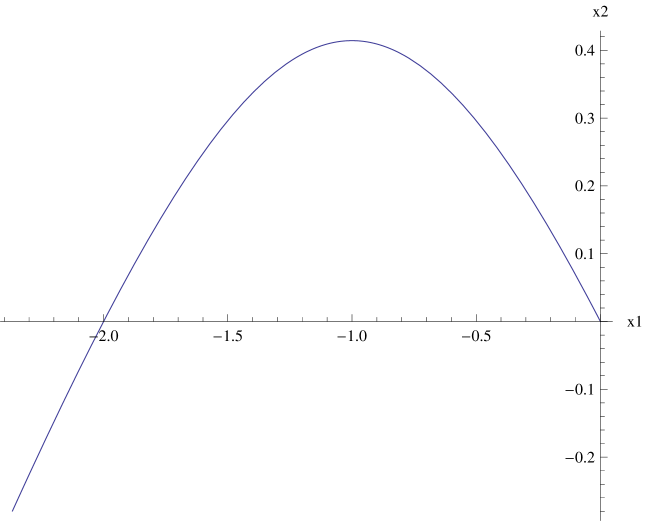
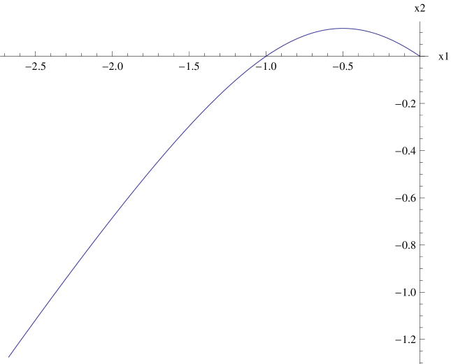
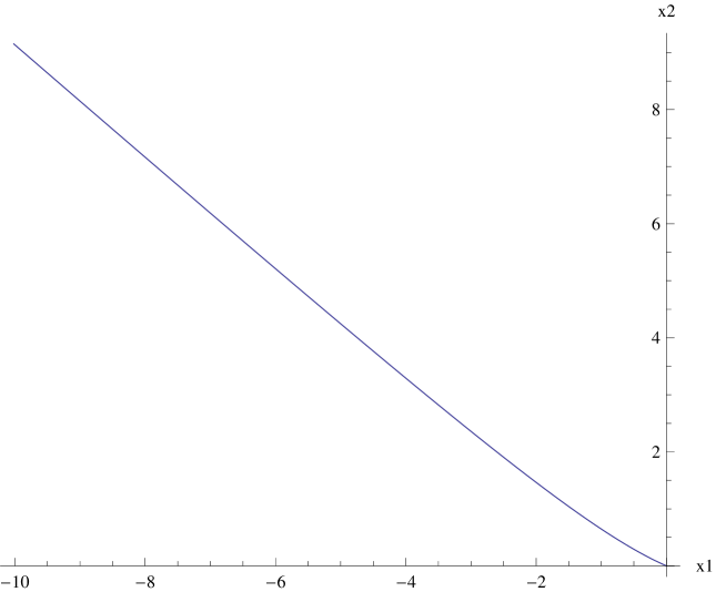
Figure 1: Projections of geodesics to the plane $(x_{1},x_{2})$ when $\xi_{3}\neq 0,\ \xi_{4}=0$

From this theorem, we obtain a description of the reachable set by geodesics $\xi_{3}\neq 0,\xi_{4}=0$ starting from the origin.

Corollary 4.8.

In the case of $\xi_{3}\neq 0,\xi_{4}=0$, let $(x_{1},x_{2},y,z)$ be a point on a time-like geodesic, then we have

$$-1<\frac{4y}{-x_{1}^{2}+x_{2}^{2}}<1.$$

Proof.

By (4.25) and (4.26), we get

$$-x_{1}^{2}+x_{2}^{2}=4(A_{2}^{2}-A_{1}^{2})\sinh^{2}\left(\frac{\xi_{3}}{2}\right),$$ (4.29)

substituting (4.29) into (4.27), we obtain the following equation:

$$y=\frac{(-x_{1}^{2}+x_{2}^{2})(\xi_{3}-\sinh(\xi_{3}))}{8\sinh^{2}\left(\frac{\xi_{3}}{2}\right)},$$ (4.30)

if we set $\tau=\frac{\xi_{3}}{2}$, then

$$y=\frac{(-x_{1}^{2}+x_{2}^{2})}{4}\left(\frac{\tau}{\sinh^{2}(\tau)}-{\coth(\tau)}\right),$$ (4.31)

or

$$\frac{4y}{(-x_{1}^{2}+x_{2}^{2})}=\frac{\tau}{\sinh^{2}(\tau)}-{\coth(\tau)}.$$ (4.32)

It is easy to check that the right hand side of (4.32) is a decreasing function in $(-\infty,+\infty),$ and its range is $(-1,1).$ That is to say, the points on the time-like geodesics should satisfy

$$-1<\frac{4y}{-x_{1}^{2}+x_{2}^{2}}<1.$$

This ends the proof. ∎

Next, we consider the case $\xi_{4}\neq 0$. Recall that

$$\dot{\zeta}_{1}=\beta\zeta_{2},\ \ \dot{\zeta}_{2}=\beta\zeta_{1},\ \ \hbox{where}\ \ \beta(s)=-(\xi_{3}+x_{1}\xi_{4}),\ \ \dot{\beta}=\xi_{4}\zeta_{1}.\$$ (4.33)

Combining the expressions for $\dot{\beta}$ and $\dot{\zeta}_{2}$ to get

$$\xi_{4}\dot{\zeta}_{2}=\beta\xi_{4}\zeta_{1}=\beta\dot{\beta}.$$ (4.34)

Integrating both sides, we have

$$\xi_{4}\zeta_{2}=\frac{\beta^{2}}{2}+C_{1},\ \ \hbox{where}\ \ C_{1}=\xi_{4}\zeta_{2}(0)-\frac{\beta^{2}(0)}{2}=\xi_{4}\xi_{2}^{0}-\frac{\xi_{3}^{2}}{2}.$$ (4.35)

This yields

$$x_{1}(s)=-\frac{\beta(s)+\xi_{3}}{\xi_{4}},$$ (4.36)

and

$$\zeta_{2}(s)=\frac{1}{\xi_{4}}\left(\frac{\beta^{2}(s)}{2}+C_{1}\right).$$ (4.37)

Since $\dot{x}_{2}=\zeta_{2},$ we deduce

$$x_{2}(s)=\int_{0}^{s}\zeta_{2}(t)dt=\frac{1}{\xi_{4}}\int_{0}^{s}\left(\frac{\beta^{2}(t)}{2}+C_{1}\right)dt.$$ (4.38)

To compute $y(s)$ in term of $\beta(s)$, we note that

$$\dot{y}=\frac{1}{2}(x_{1}\zeta_{2}+x_{2}\zeta_{1})=\frac{1}{2}(x_{1}\dot{x}_{2}-x_{2}\dot{x}_{1}),$$ (4.39)

then integration by parts yields

$$y(s) =\frac{1}{2}\int_{0}^{s}(x_{1}\dot{x}_{2}-x_{2}\dot{x}_{1})dt=\int_{0}^{s}x_{1}\zeta_{2}dt-\frac{1}{2}x_{1}x_{2}$$

$$=-\frac{1}{\xi_{4}^{2}}\int_{0}^{s}\left({\beta(t)+\xi_{3}}\right)\left(\frac{\beta^{2}(t)}{2}+C_{1}\right)dt-\frac{1}{2}x_{1}x_{2}.$$ (4.40)

Finally, since $\dot{z}=\frac{x_{1}^{2}+x_{2}^{2}}{2}\zeta_{2},$

$$z(s) =\int_{0}^{s}\frac{x_{1}^{2}+x_{2}^{2}}{2}\zeta_{2}dt=\frac{1}{2}\int_{0}^{s}x_{1}^{2}\zeta_{2}dt+\frac{1}{6}x_{2}^{3}$$

$$=\frac{1}{2\xi_{4}^{3}}\int_{0}^{s}\left({\beta(t)+\xi_{3}}\right)^{2}\left(\frac{\beta^{2}(t)}{2}+C_{1}\right)dt+\frac{1}{6}x_{2}^{3}.$$ (4.41)

Once we find $\beta$, we can find the geodesic $(x_{1}(s),x_{2}(s),y(s),z(s))$ explicitly.

Since $\dot{\beta}(s)=\xi_{4}\zeta_{1}$, $\dot{\beta}(0)=\xi_{4}\zeta_{1}(0)=\xi_{4}\xi_{1}^{0}$, we have

$$\ddot{\beta}(s)=\xi_{4}\dot{\zeta}_{1}=\xi_{4}\beta(s)\zeta_{2}=\beta(s)(\xi_{4}\zeta_{2})=\beta(s)\left(\frac{\beta^{2}(s)}{2}+C_{1}\right).$$ (4.42)

Multiplying both sides by $2\dot{\beta}(s)$ and integrating, we have

$$\dot{\beta}^{2}(s)=\frac{\beta^{4}(s)}{4}+C_{1}\beta^{2}(s)+C_{2}=\left(\frac{\beta^{2}(s)}{2}+C_{1}\right)^{2}+C_{2}-C_{1}^{2},$$ (4.43)

where $C_{2}$ is a constant, and

$$C_{2}=\dot{\beta}^{2}(0)-\frac{\beta^{4}(0)}{4}-C_{1}\beta^{2}(0)=(\xi_{1}^{0})^{2}\xi_{4}^{2}+\frac{\xi_{3}^{4}}{4}-\xi_{2}^{0}\xi_{3}^{2}\xi_{4}.$$ (4.44)

Then

$$C_{2}-C_{1}^{2}=(\xi_{1}^{0})^{2}\xi_{4}^{2}+\frac{\xi_{3}^{4}}{4}-\xi_{2}^{0}\xi_{3}^{2}\xi_{4}-\left(\xi_{2}^{0}\xi_{4}-\frac{\xi_{3}^{2}}{2}\right)^{2}=\xi_{4}^{2}((\xi_{1}^{0})^{2}-(\xi_{2}^{0})^{2})=\xi_{4}^{2},$$ (4.45)

since $(\xi_{1}^{0})^{2}-(\xi_{2}^{0})^{2}=1$.

Assume $\dot{\beta}(s)>0$, we have

$$\frac{d\beta(s)}{ds}=\sqrt{\left(\frac{\beta^{2}(s)}{2}+C_{1}\right)^{2}+\xi_{4}^{2}}.$$ (4.46)

Hence

$$ds=\frac{d\beta}{\sqrt{\left(\frac{\beta^{2}(s)}{2}+C_{1}\right)^{2}+\xi_{4}^{2}}}.$$ (4.47)

Let $\rho^{2}=C_{1}+\xi_{4}i$, $\bar{\rho}^{2}=C_{1}-\xi_{4}i$ and $u=\frac{\beta}{\sqrt{2}}$, integrating (4.47) from $0$ to $s$, we obtain

$$s=\int_{\frac{\beta(0)}{\sqrt{2}}}^{\frac{\beta(s)}{\sqrt{2}}}\frac{\sqrt{2}du}{\sqrt{(u^{2}+\rho^{2})(u^{2}+\bar{\rho}^{2})}}.$$ (4.48)

Set

$$k^{2}=-\frac{(\rho-\bar{\rho})^{2}}{4\rho\bar{\rho}}=\frac{\sqrt{C_{1}^{2}+\xi_{4}^{2}}-C_{1}}{2\sqrt{C_{1}^{2}+\xi_{4}^{2}}},$$

$$\mathfrak{g}=\frac{1}{2\sqrt{\rho\bar{\rho}}}=\frac{1}{2(C_{1}^{2}+\xi_{4}^{2})^{\frac{1}{4}}}.$$

Since

$$\int_{y}^{\infty}\frac{dt}{\sqrt{(t^{2}+\rho^{2})(t^{2}+\bar{\rho})}}=\mathfrak{g}\cdot cn^{-1}\ (cos\ \varphi,k)=\mathfrak{g}F(\varphi,k),$$ (4.49)

where $cn^{-1}\ (y,k)$ is a Jacobi’s Inverse Elliptic Functions, and

$$\varphi=\cos^{-1}\ \left(\frac{y^{2}-\rho\bar{\rho}}{y^{2}+\rho\bar{\rho}}\right),\ \ \ F(\varphi,k)=\int_{0}^{\varphi}\frac{dt}{\sqrt{1-k^{2}sin^{2}\ t}}.$$

Hence

$$\int_{\frac{\beta(0)}{\sqrt{2}}}^{\frac{\beta(s)}{\sqrt{2}}}\frac{\sqrt{2}du}{\sqrt{(u^{2}+\rho^{2})(u^{2}+\bar{\rho}^{2})}}=\int_{\frac{\beta(0)}{\sqrt{2}}}^{\infty}\frac{\sqrt{2}du}{\sqrt{(u^{2}+\rho^{2})(u^{2}+\bar{\rho}^{2})}}-\int_{\frac{\beta(s)}{\sqrt{2}}}^{\infty}\frac{\sqrt{2}du}{\sqrt{(u^{2}+\rho^{2})(u^{2}+\bar{\rho}^{2})}}.$$

According to (4.49), we have

$$\int_{\frac{\beta(0)}{\sqrt{2}}}^{\infty}\frac{\sqrt{2}du}{\sqrt{(u^{2}+\rho^{2})(u^{2}+\bar{\rho}^{2})}}=\sqrt{2}\mathfrak{g}F(\varphi_{1},k)=constant,$$ (4.50)

where

$$\varphi_{1}=cos^{-1}\ \left(\frac{\xi_{3}^{2}-2\sqrt{C_{1}+\xi_{4}^{2}}}{\xi_{3}^{2}+2\sqrt{C_{1}+\xi_{4}^{2}}}\right).$$

Since

$$\int_{\frac{\beta(s)}{\sqrt{2}}}^{\infty}\frac{\sqrt{2}du}{\sqrt{(u^{2}+\rho^{2})(u^{2}+\bar{\rho}^{2})}}=\sqrt{2}\mathfrak{g}\cdot cn^{-1}\ \left(\frac{\beta^{2}(s)-2\rho\bar{\rho}}{\beta^{2}(s)+2\rho\bar{\rho}}\right).$$ (4.51)

Hence

$$cn^{-1}\ \left(\frac{\beta^{2}(s)-2\rho\bar{\rho}}{\beta^{2}(s)+2\rho\bar{\rho}}\right)=F(\varphi_{1},k)-\frac{s}{\sqrt{2}\mathfrak{g}},$$ (4.52)

let $F=F(\varphi_{1},k),$ we obtain

$$\beta^{2}(s)=\frac{2\rho\bar{\rho}\left(1+cn\ \left(F-\frac{s}{\sqrt{2}\mathfrak{g}},k\right)\right)}{\left(1-cn\ \left(F-\frac{s}{\sqrt{2}\mathfrak{g}},k\right)\right)}=\frac{2\rho\bar{\rho}\left(1+cn\ \left(2\tilde{s},k\right)\right)}{\left(1-cn\ \left(2\tilde{s},k\right)\right)},$$ (4.53)

where $2\tilde{s}=F-\frac{s}{\sqrt{2}\mathfrak{g}}$.

Since

$$\frac{1-cn\ (2s)}{1+cn\ (2s)}=tn^{2}\ (s)dn^{2}\ (s),$$ (4.54)

hence

$$\beta(s)=\frac{\sqrt{2\rho\bar{\rho}}}{tn\ (\tilde{s},k)dn\ (\tilde{s},k)}=\sqrt{2\rho\bar{\rho}}cs\ (\tilde{s},k)nd\ (\tilde{s},k).$$ (4.55)

For the case of $\dot{\beta}(s)<0,$ we can calculate by the same method, and get the same result. But the expression of the parameter $\tilde{s}$ in (4.53) and(4.55) should be changed to

$$\frac{1}{2}\left(F+\frac{s}{\sqrt{2}\mathfrak{g}}\right).$$

Thus the sign of $\dot{\beta}(s)$ will not affect the expression of the geodesics.

Therefore, integrating equations (4.36), (4.38), (4.40) and (4.41), we get a complete description of the Hamiltonian time-like geodesics in the Engel group.

Theorem 4.9.

In the case of $\xi_{4}\neq 0$, time-like geodesics starting from the origin are given by:

$$x_{1}(s)=-\frac{1}{\xi_{4}}(\beta(s)+\xi_{3}),$$ (4.56)

$$x_{2}(s)=\frac{1}{2\xi_{4}}(B_{2}(s)+2C_{1}),$$ (4.57)

$$y(s)=-\frac{1}{2\xi_{4}^{2}}(B_{3}(s)+2C_{1}B_{1}(s)+\xi_{3}B_{2}(s)+2C_{1}\xi_{3}s)-\frac{1}{2}x_{1}(s)x_{2}(s),$$ (4.58)

$$z(s)=\frac{1}{4\xi_{4}^{3}}(B_{4}(s)+2C_{1}B_{2}(s)+2\xi_{3}B_{3}(s)+4C_{1}\xi_{3}B_{1}(s)+\xi_{3}^{2}B_{2}(s)+2C_{1}\xi_{3}^{2})+\frac{1}{6}x_{2}^{3}(s),$$ (4.59)

where $C_{1}=\xi_{4}\xi_{2}^{0}-\frac{\xi_{3}^{2}}{2}$, $B_{i}(s)=\int^{s}_{0}\beta^{i}(t)dt,\ i=1,\ldots,4,$ and the expressions of $B_{i}(s)$ are presented in Appendix.

Projections of geodesics to the plane $(x_{1},x_{2})$ with $\xi(0)=(1,0,1,1)$,  $\xi(0)=(\frac{\sqrt{5}}{2},1/2,2,1)$ and $\xi(0)=(\frac{\sqrt{5}}{2},1/2,1,1)$ are shown in Figure 2.

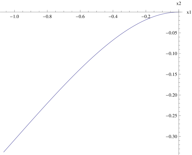
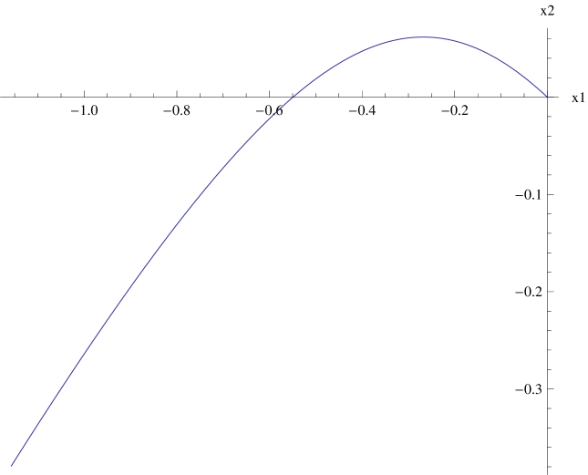
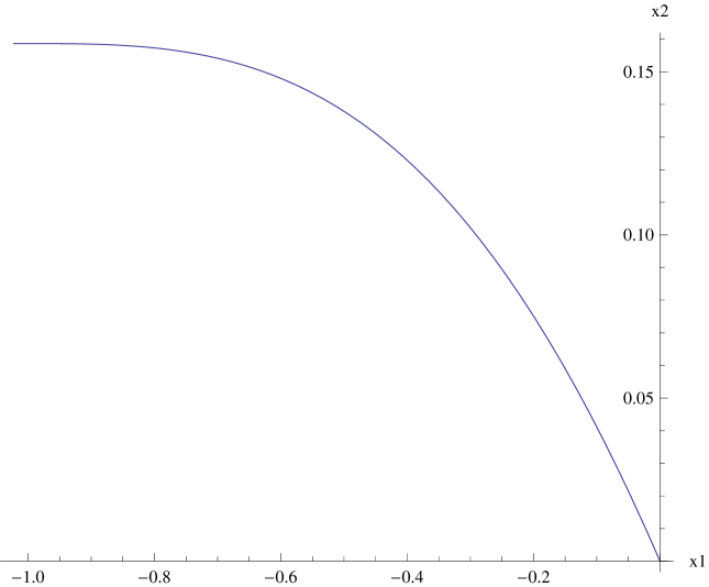
Figure 2: Projections of geodesics to the plane $(x_{1},x_{2})$ when $\xi_{3}\neq 0,\ \xi_{4}\neq 0$

Appendix

Denoting

$$\psi_{1}(s)=ln\ (k^{\prime 2}+cs^{2}\ (s,k)), \psi_{2}(s)=\frac{dn\ (2s,k)sn\ (2s,k)}{(1-cn\ (2s,k))^{2}},$$

$$\psi_{3}(s)=\frac{E(2s,k)-E(2s,k)cn\ (2s,k)}{1-cn\ (2s,k)}, F(\varphi,k)=\int_{0}^{\varphi}\frac{dt}{\sqrt{1-k^{2}sin^{2}\ t}},$$

$$k^{2}=\frac{\sqrt{C_{1}^{2}+\xi_{4}^{2}}-C_{1}}{2\sqrt{C_{1}^{2}+\xi_{4}^{2}}},\ \ \ \ \ \ \mathfrak{g}=\frac{1}{2(C_{1}^{2}+\xi_{4}^{2})^{\frac{1}{4}}},\ \ \ \ \ \ \varphi_{1}=cos^{-1}\ \left(\frac{\xi_{3}^{2}-2\sqrt{C_{1}+\xi_{4}^{2}}}{\xi_{3}^{2}+2\sqrt{C_{1}+\xi_{4}^{2}}}\right)$$

we get the expressions of $B_{i}(s)$ as following:

$$B_{1}(s) =\int^{s}_{0}\beta(t)dt=\mathfrak{g}\psi_{1}(\tilde{s})+D_{1},$$

$$B_{2}(s) =\int^{s}_{0}\beta^{2}(t)dt=\frac{\sqrt{2}}{\mathfrak{g}}[-3\tilde{s}+(1-cn\ (2\tilde{s},k))\psi_{2}(\tilde{s})+\psi_{3}(\tilde{s})]+D_{2},$$

$$B_{3}(s) =\int^{s}_{0}\beta^{3}(t)dt=\frac{1}{2\mathfrak{g}^{2}k^{\prime 2}}[k^{\prime 2}cs^{2}\ (\tilde{s},k)+k^{\prime 2}(2k^{2}-1)\psi_{1}(\tilde{s})-(2k^{4}-k^{6}-k^{2})e^{\psi_{1}(\tilde{s})}]+D_{3},$$

$$B_{4}(s) =\int^{s}_{0}\beta^{4}(t)dt=\frac{\sqrt{2}}{3\mathfrak{g}^{3}}[-\frac{3}{2}\tilde{s}+(3-4k^{2})\psi_{2}(\tilde{s})+4k^{\prime 2}(1+k^{2})\tilde{s}-2k^{\prime 2}E(2\tilde{s},k)]+D_{4},$$

where $\tilde{s}=\frac{1}{2}\left(F\pm\frac{s}{\sqrt{2}\mathfrak{g}}\right)$, $F=F(\varphi_{1},k)$, $D_{1},D_{2},D_{3},D_{4}$ are constants, and

$$D_{1} =-\mathfrak{g}\psi_{1}\left(\frac{F}{2}\right),$$

$$D_{2} =\frac{\sqrt{2}}{\mathfrak{g}}\left[\frac{3F}{2}-(1-cn\ (F,k))\psi_{2}\left(\frac{F}{2}\right)-\psi_{3}\left(\frac{F}{2}\right)\right],$$

$$D_{3} =\frac{1}{2\mathfrak{g}^{2}k^{\prime 2}}\left[-k^{\prime 2}cs^{2}\ \left(\frac{F}{2},k\right)-k^{\prime 2}(2k^{2}-1)\psi_{1}\left(\frac{F}{2}\right)+(2k^{4}-k^{6}-k^{2})e^{\psi_{1}\left(\frac{F}{2}\right)}\right],$$

$$D_{4} =\frac{\sqrt{2}}{3\mathfrak{g}^{3}}\left[\frac{3F}{4}-(3-4k^{2})\psi_{2}\left(\frac{F}{2}\right)-2k^{\prime 2}(1+k^{2})F+2k^{\prime 2}E(F,k)\right].$$

Acknowledgement

This work was supported by NSFC(No.11071119, No.11401531) and NSFC-RFBR (No. 11311120055). The authors cordially thank the referees for their careful reading and helpful comments.

References

- [1] A.A. Agrachev, El-H. Chakir El-A.,and J. P. Gauthier, Sub-Riemannian metrics on , Proc. Conf. Canad. Math. Soc. 25(1998).
- [2] A. Agrachev, D. Barilari, and U. Boscain, On the Hausdorff volume in sub-Riemannian geometry, Calculus of Variations and Partial Differential Equations 10.1007/s00526-011-0414-y (2011), 1–34.
- [3] A. Agrachev, U. Boscain, J.-P. Gauthier, and F. Rossi, The intrinsic hypoelliptic Laplacian and its heat kernel on unimodular Lie groups, J. Funct. Anal. 256(2009), No. 8, 2621–2655.
- [4] A. A. Agrachev, G. Charlot, J. P. A. Gauthier, and V. M. Zakalyukin, On sub-Riemannian caustics and wave fronts for contact distributions in the three-space, J. Dynam. Control Systems 6 (2000), No. 3, 365-395.
- [5] A. Ardentov, Yu. Sachkov, Extremal trajectories in a nilponent sub-Riemannian problem on the Engel group, Matematicheskii Sbornik 202(2011), No. 11, 31-54.
- [6] A. Ardentov, Yu. Sachkov, Conjugate points in nilpotent sub-Riemannian problem on the Engel group, Journal of Mathematical Sciences 195(2013), No. 3, 369-390.
- [7] A.Ardentov, Yu. L. Sachkov, Cut time in sub-Riemannian problem on Engel group, ESAIM: Control, Optimisation and Calculus of Variations, accepted.
- [8] Cartan, , Sur quelques quadratures clout l’elernent diflerentiel contient des fonctions arbitraires, Bull. Soc. Math. France29(1901), 118-130.
- [9] El-H. Alaoui, J-P. Gauthier, and I. Kupka, Small sub-Riemannian balls in , J. Dynam. Control Sys. 2(1996), No.3, 359-421.
- [10] R. Beals, B. Gaveau, and P.C. Greiner, Hamilton-Jacobi theory and the Heat Kernal on Heisenberg groups, J. Math. Pures Appl.79,7(2000)633-689.
- [11] J.K. Beem, P.E. Ehrlich, and K.l. Easley, Global Lorentzian geometry, Marcel Dekker(1996).
- [12] D. C. Chang, I. Markina, and A. Vasiliev, Sub-Lorentzian geometry on anti-de Sitter space, J. Math. Pures Appl.90(2008),No.1,82-110.
- [13] M. Golubitsky and V. Guillemin, Stable mappings and their singularities, Spinger-Verlag, New York(1973).
- [14] M. Grochowski, Differential properties of the sub-Riemannian distance function, Bull. Polish. Acad. Sci. 50(2002),No.1.
- [15] M. Grochowski, Geodesics in the sub-Lorentzian geometry, Bull. Polish. Acad. Sci. 50(2002), No.2.
- [16] M. Grochowski, Normal forms of germs of Contact sub-Lorentzian structures on , Differentiability of the sub-Lorentzian distance function, J. Dynam. Control Sys. 9(2003), No.4, 531-547.
- [17] M. Grochowski, Reachable sets for the Heisenberg sub-Lorentzian structure on , an estimate for the distance function, J. Dynam. Control Sys.12(2006), No.2, 145-160.
- [18] M. Grochowski, On the Heisenberg sub- Lorentzian Metric on , Geometric Singularity Theory, Banach Center Publications, 65(2004).
- [19] M. Gromov, Carnot-Carath eodory spaces seen from within, Progr. Math. 144, Birkh auser, Boston (1996), 79-323.
- [20] Tiren Huang, Xiaoping Yang, Geodesics in the Heisenberg Group with a Lorentzian metric, J. Dynam. Control Sys.18(2012), No.1, 21-40.
- [21] F. Monroy-Prez, and A. Anzaldo-Meneses, Optimal control on the Heisenberg group, J. Dynam. Control Sys. 5(1996), No.4, 473-499.
- [22] B. O’Neill, Semi-Riemannian Geometry: with Applications to Relativity, Pure and Applied Mathematics, vol. 103, Academic Press, Inc., New York, 1983.
- [23] A. Korolko, and I. Markina, Non-Holonomic Lorentzian geometry on some -type groups, J. Geom. Anal.19(2009)864-889.
- [24] R. Montgomery, Singular extremals on Lie groups, Math. Control, Signals and Systems vol. 7(3)(1994)217-234.
- [25] R. Montgomery, A tour of sub-Riemannian geometries, their geodesics and applications, Math. Surveys and Monographs 91, American Math. Soc., Providence, 2002.
- [26] P. Piccione, and D.V. Tausk, Variational aspects of the geodesic problem in sub-Riemannian geometry, J. Geometry and Physics. 39(2001)183-206.
- [27] Yu. L. Sachkov, Conjugate and cut time in the sub-Riemannian problem on the group of motions of a plane, ESAIM Control Optim. Calc. Var.16 (2010), 1018-1039.
- [28] H. J. Sussmann, An extension of a theorem of Nagano on transitive Lie algebras, Proc. Am. Math. Soc. 45 (1974), 349-356.
- [29] R. Strichartz, Sub-Riemannian geometry, J. Diff. Geom. 24(1986)221-263.