Enhancement and Suppression of Four wave mixing in coupled semiconductor quantum dot-gold grating systems.

Abstract

We have shown that Four wave mixing (FWM) processes of electromagnetic field modes of a grating can be controlled by the presence of interactions with a quantum dot or a molecule made by coupled quantum dots. By choosing the appropritae level spacing for the quantum emitter, one can either suppress or enhance the Four wave mixing process. We revel theoretically the underlying mechanism for this effect. (i) Suppression in FWM intensity occurs simply because induced Electromagnetic Induced Transparency does not allow the excitation at converted FWM frequency. (ii) Enhancement emerges since FWM process can be brought to resonance. Path interference effect cancels the nonresonant frequency terms. Furthermore, we have also shown that in case of coupled quantum dots enhancement increases significantly as compared to the case of a single quantum dot.

I Introduction

Quantum Plasmonics is an emerging area of research which involves the study of the optical properties of hybrid photonic structures incorporating both plasmonic nanostructures and quantum emitters Tame , such as atoms, molecules and semiconductor quantum dots. These complex hybrid are active photonic structures and expected to enhance optical response significantly, for example modification of the linear susceptibility Lu ; Hatef ; Sadeghi ; Paspalakis ; Tasgin and the enhancement of nonlinear susceptibilities in several quantum systems with different level structures coupled to various plasmonic nanostrcutures Lu1 ; Pu ; Paspalakis1 ; Singh ; Paspalakis2 .

Four Wave Mixing is one of the above mentioned nonlinear process of light-matter interactions in which three incoming waves,indicated as $\omega_{1}$, $\omega_{2}$, $\omega_{3}$ in the material generate a fourth wave of frequency $\omega_{4}$ Yurke . Assuming that the three incident waves have frequencies in the visible or near-infrared range, the incoming electric fields $E\left(\omega_{i}\right)$ $($with $i=1,2,3)$ interact with the material’s electrons to induce a nonlinear polarization $P^{\left(3\right)}\left(\omega_{4}\right)$ in the illuminated volume. The magnitude of the polarization is determined by the strength of the incident fields and the efficiency with which the material can be polarized Wang . The latter is indicated with the third-order nonlinear susceptibility $\chi^{\left(3\right)}$, a measure of the material’s response to the incoming fields. Four wave mixing (FWM) has found numerous practical applications, including: optical processing; nonlinear imaging; real-time holography and phase-conjugate optics; phase-sensitive amplification; and entangled photon pair production Scully .

In several recent studies, the modification of $\chi^{\left(3\right)}$ (FWM process) susceptibility in a quantum dot system coupled to spherical nanoparticle has been investigated when the hybrid structures interacts with a weak probe field and a strong pump field Lu1 ; Li ; Liu ; Li1 . All these works have shown for different distance between the quantum dot and the metal nanoparticle the $\chi^{\left(3\right)}$ susceptibility can be either enhanced or strongly suppressed. In addition, bistable behavior has been also reported in these kind of systems Paspalakis2 ; Li .

Here, we propose a method for increasing the efficiency of FWM processes by exploiting gold grating Jan ; Poutrina . Narrow peaks are observed in the transmission spectra of p-polarized light passing through a thin gold film that is coated on the surface of a transparent diffraction grating. The spectral position and intensity of these peaks can be tuned over a wide range of wavelengths by simple rotation of the grating Bipin . The wavelengths where these transmission peaks are observed correspond to conditions where surface plasmon resonance occurs at the gold-air interface. Light diffracted by the grating couples with surface plasmons in the metal film to satisfy the resonant condition, resulting in enhanced light transmission through the film.

The paper is organized as follows. In Section II, we describe the FWM Process in the coupled system of gold grating with a quantum oscillator. In the same section, we introduce the Hamiltonian for hybrid system. FWM process is also included in the second quantized Hamiltonian. We derive the equations of motion for the system using the density matrix formalism for the quantized quantum oscillator. We use phenomenological way to include damping of gold grating modes as well as quantum emitter. In Section II B, We demonstrated that FWM process can be suppressed for $\left(\omega_{eg}=2\omega-\omega^{\prime}\right)$. In Section II C, we present a contrary effect where FMW process can be enhanced. This is due to cancellation of non resonant terms in denominator. In Section III, we further investigate the case of gold grating coupled to two quantum emitters (both quantum emitters coupled to each other also) simultaneously. We conclude our results in Section IV.

II Hamiltonian for Four Wave Mixing

The total Hamiltonian $\hat{H}$  for the described system can be written as Sum of the energy of the Quantum Oscillator $\hat{H}_{0}$,( In our case we have taken a QD of energy levels $\left|e\right\rangle~{}$and $\left|g\right\rangle$) , enegy of the elctromagnetic modes of Gold Grating $\left(\hat{a}_{1},\hat{a}_{2},\hat{a}_{3}\right)$ for a particular angle of incidence of Pump lasers $\hat{H}_{grating}$, the interaction of the Quantum Oscillator with the Grating Modes $\hat{H}_{int}$

$$\hat{H}_{0}=\hbar\omega_{e}\left|e\right\rangle\left\langle e\right|+\hbar\omega_{g}\left|g\right\rangle\left\langle g\right|$$ (1)

$$\hat{H}_{grating}=\hbar\omega_{1}\hat{a}_{1}^{\dagger}\hat{a}_{1}+\hbar\omega_{2}\hat{a}_{2}^{\dagger}\hat{a}_{2}+\hbar\omega_{3}\hat{a}_{3}^{\dagger}\hat{a}_{3}$$ (2)

$$\hat{H}_{int}=\hbar\left(f~{}\hat{a}_{3}^{\dagger}\left|g\right\rangle\left\langle e\right|+f~{}^{\ast}\hat{a}_{3}\left|e\right\rangle\left\langle g\right|\right)$$ (3)

Here, we have considered that level spacing of the QD is only resonant to $\hat{a}_{3}$ mode (i.e. $\omega_{eg}\sim\omega_{3}$). as well as the energy transferred by the pump source $\omega$ and $\omega^{\prime}.$

$$\hat{H}_{P}=i\hbar\left(\hat{a}_{1}^{\dagger}~{}\epsilon_{P}e^{-i\omega t}-\hat{a}_{1}~{}\epsilon_{P}^{\ast}e^{i\omega t}\right)+i\hbar\left(\hat{a}_{2}^{\dagger}~{}\epsilon_{P}^{\prime}e^{-i\omega^{\prime}t}-\hat{a}_{2}~{}\epsilon_{P}^{\ast\prime}e^{i\omega^{\prime}t}\right)$$ (4)

$$\hat{H}_{FWM}=\hbar\chi^{(2)}\left(\hat{a}_{3}^{\dagger}\hat{a}_{2}^{\dagger}\hat{a}_{1}^{2}+\hat{a}_{1}^{\dagger 2}\hat{a}_{2}\hat{a}_{3}~{}\right)$$ (5)

For the Process of $\left(\omega_{3}=~{}2\omega_{1}-\omega_{2}\right)~{}$as mentioned in PRL 103, 266802.

In Eq. (1), $\hbar\omega_{e}$ ($\hbar\omega_{g}$) is the excited (ground) state energy of the Quantum Oscillator.  States $\left|e\right\rangle$ and $\left|g\right\rangle$ corresponds to excited and ground levels of the Quantum Oscillator respectively.  $\left(\hat{a}_{1},\hat{a}_{2},\hat{a}_{3}\right)$ are the Gold Grating modes at a particulat angle of incidence $\theta=5^{\circ}$. $f~{}$ is the coupling matrix element between the field of grating mode and the Quantum Oscillator. Eq. (4) describes the driving the Electromagnetic field modes of grating $\left(\hat{a}_{1}\text{ and }\hat{a}_{2}\right)$ with $e^{-i\omega t}$ and $e^{-i\omega^{\prime}t}$ respectively.

Eq.(5) describes where the Four wave mixing takes place in which $\hat{a}_{1}$ mode contributes two photons and $\hat{a}_{2}$ mode single photons in the process.

II.1 Heisenberg Equations of Motion

We use the commutation relations

$$i\hbar\frac{d}{dt}\hat{O}=\left[\hat{O},\hat{H}\right]$$ (6)

for deriving equations of motions. After obtaining the dynamics in the quantum approach, we carry $\left(\hat{a}_{1},\hat{a}_{2},\hat{a}_{3}\right)~{}$to classical expectation values $\left(\alpha_{1},\alpha_{2},\alpha_{3}\right).~{}$We also introduce the decay rates for $\left(\alpha_{1},\alpha_{2},\alpha_{3}\right).$ Quantum Oscillator is treated within the density matrix approach. The equations of motion take the form

$$\dot{\alpha}_{1}=\left(-i\omega_{1}-\gamma_{1}\right)\alpha_{1}-2i\chi^{\left(3\right)}\alpha_{1}^{\ast}\alpha_{2}\alpha_{3}+\epsilon_{p}e^{-i\omega t}$$ (7a)

$$\dot{\alpha}_{2}=\left(-i\omega_{2}-\gamma_{2}\right)\alpha_{2}-i\chi^{\left(3\right)}\alpha_{3}^{\ast}\alpha_{1}^{2}+\epsilon_{p}^{\prime}e^{-i\omega^{\prime}t}$$ (7b)

$$\dot{\alpha}_{3}=\left(-i\omega_{3}-\gamma_{3}\right)\alpha_{3}-i\chi^{\left(3\right)}\alpha_{2}^{\ast}\alpha_{1}^{2}-if\rho_{ge}$$ (7c)

$$\dot{\rho}_{ge}=\left(-i\omega_{eg}-\gamma_{eg}\right)\rho_{ge}+if\alpha_{3}\left(\rho_{ee}-\rho_{gg}\right)$$ (7d)

$$\dot{\rho}_{ee}=-\gamma_{ee}\rho_{ee}+~{}if\left(\alpha_{3}^{\ast}\rho_{ge}-\alpha_{3}\rho_{eg}\right)$$ (7e)

where $$\gamma_{1} \gamma_{2},\gamma_{3}~{} \left(\alpha_{1},\alpha_{2},\alpha_{3}\right).~{}\gamma_{ee}~{} \gamma_{eg}= \gamma_{ee}/2~{} \rho_{ee}+~{}\rho_{gg}=1$$,are the damping rates of the electromagnetic modes of the gold grating and are the diagonal and off-diagonal elements of the quantum oscillator respectively. The constraints of the conservation probability accompanies above set of equations.

Besides the time-evolution simulations, one may gain the understanding by seeking solutions of the following form. For long time behavior we take solutions of the form

$\alpha_{1}(t)=\tilde{\alpha}_{1}e^{-i\omega t},\alpha_{2}(t)=\tilde{\alpha}_{2}e^{-i\omega^{\prime}t},\alpha_{3}(t)=\tilde{\alpha}_{3}e^{-i\left(2\omega-\omega^{\prime}\right)t}$ (Condition of Four wave mixing process), $\rho_{ge}=\tilde{\rho}_{ge}e^{-i\left(2\omega-\omega^{\prime}\right)t}$ here we have considered that level spacing of the QD is only resonant to $\hat{a}_{3}$ mode (i.e. $\omega_{eg}\sim\omega_{3}$), $\rho_{ee}=\tilde{\rho}_{ee}.$

Inserting the solutions in above set of equations (7a-7e) we have for long time behavior

$$\left[i\left(\omega_{1}-\omega\right)+\gamma_{1}\right]\tilde{\alpha}_{1}+2i\chi^{\left(3\right)}\tilde{\alpha}_{1}^{\ast}\tilde{\alpha}_{2}\tilde{\alpha}_{3}=\epsilon_{p}$$ (8a)

$$\left[i\left(\omega_{2}-\omega^{\prime}\right)+\gamma_{2}\right]\tilde{\alpha}_{2}+i\chi^{\left(3\right)}\tilde{\alpha}_{3}^{\ast}\tilde{\alpha}_{1}^{2}=\epsilon_{p}^{\prime}$$ (8b)

$$\left[i\left(\omega_{3}+\omega^{\prime}-2\omega\right)+\gamma_{3}\right]\tilde{\alpha}_{3}+i\chi^{\left(3\right)}\tilde{\alpha}_{2}^{\ast}\tilde{\alpha}_{1}^{2}=-if\tilde{\rho}_{ge}$$ (8c)

$$\left[i\left(\omega_{eg}+\omega^{\prime}-2\omega\right)+\gamma_{eg}\right]\tilde{\rho}_{ge}=if\tilde{\alpha}_{3}\left(\tilde{\rho}_{ee}-\tilde{\rho}_{gg}\right)$$ (8d)

$$\gamma_{ee}\tilde{\rho}_{ee}=if\left(\tilde{\alpha}_{3}^{\ast}\tilde{\rho}_{ge}-\tilde{\alpha}_{3}\tilde{\rho}_{eg}\right)$$ (8e)

Using equations (8c) and (8d), we obtain the steady state value for $$\tilde{\alpha}_{3}$$ as follows

$$\tilde{\alpha}_{3}=\frac{i\chi^{\left(3\right)}\tilde{\alpha}_{2}^{\ast}\tilde{\alpha}_{1}^{2}}{\frac{\left|f\right|^{2}y}{\left[i\left(\omega_{eg}+\omega^{\prime}-2\omega\right)+\gamma_{eg}\right]}-\left[i\left(\omega_{3}+\omega^{\prime}-2\omega\right)+\gamma_{3}\right]}$$ (9)

Where $y=\left(\tilde{\rho}_{ee}-\tilde{\rho}_{gg}\right)$is the steady state value of the population inversion. If the quantum oscillator is tuned around $\omega_{eg}=2\omega-\omega^{\prime},$ $\tilde{\alpha}_{3}$ can be suppressed.

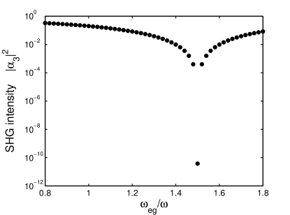
Figure 1: Suppression of the FWM intensity to the $\hat{a}_{3}$ gold grating mode from the $\hat{a}_{2}$ and $\hat{a}_{1}$ mode. Even at the presence of the resonant FWM condition, $\omega_{1}=\omega=1.0$, $\omega_{2}=\omega^{\prime}=0.5$ and $\left(\omega_{3}=2\omega-\omega^{\prime}\right)$, the presence of quantum oscillator prevents to take place of the FWM process. EIT does not allow the FWM process. The resonant FWM conversion is represented by unity in figure. When $\left(\omega_{eg}=2\omega-\omega^{\prime}\right)$, the FWM intensity even can be suppressed by 10 orders of magnitude with respect to resonant value. Decay rates for our numerical simulations are $\gamma_{1}=\gamma_{2}=\gamma_{3}=0.01\omega$ and $\gamma_{eg}=0.00001\omega$. We have taken $\chi^{\left(2\right)}=0.00001\omega$ and $f=0.1\omega$

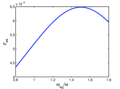
Figure 2: Enhancement of population in excited level of the quantum oscillator coupled to gold grating at the resonance condition $\left(\omega_{eg}=2\omega-\omega^{\prime}\right)$. We can see the population in excited level is maximum at this condition unlike FWM Intensity $|$ $\tilde{\alpha}_{3}$ $|^{2}$ shown in Fig. 1. All other parameters for numerical simulation remain same like in Fig 1.

II.2 Suppression of the Four wave Mixing Process

We can see from Eq. (9) that $\left|f\right|^{2}y/\gamma_{eg}$ can attain huge values on resonance $\omega_{eg}=~{}2\omega-\omega^{\prime}$as well as linewidth of the quantum oscillator $\gamma_{eg}$ is very small  compared to the all other frequencies. If $f\neq 0$, the largeness of the $\left|f\right|^{2}y/\gamma_{eg}$ term dominates the denominator. This results in the suppression of the generation of the FWM mode $\tilde{\alpha}_{3}$ in our model Hamiltonian system. In Fig.1 we have shown that FWM process can be suppressed very effectively by coupling to gold grating to quantum oscillator. We have time evolve Eqs. $\left(7a-7e\right)$ to obtain steady state values for the FWM intensity.
Without the presence of quantum oscillator, the FWM would be maximum $\tilde{\alpha}_{3}=-\frac{i\chi^{\left(3\right)}\tilde{\alpha}_{2}^{\ast}\tilde{\alpha}_{1}^{2}}{\gamma_{3}}$ when the FWM mode is on resonance $\left(\omega_{3}=2\omega-\omega^{\prime}\right)$. In Fig. 1 we observe that even at the presence of this resonance condition $\left(\omega_{3}=2\omega-\omega^{\prime}\right)$, EIT suppresses the FWM by 10 order of magnitude. Furthermore, in this case population of excited level of quantum oscillator is maximum at this point as shown in Fig.2 as well as population inversion is approximately $y=\left(\tilde{\rho}_{ee}-\tilde{\rho}_{gg}\right)\approx-1$

II.3 Enhancement of Four Wave Mixing Process

Similar to suppression phenomena, the interference effects can be arranged in such a way that FWM process can be carried closer to resonance. In the denominator of Eq.(9),  the imaginary part of the first term$~{}\frac{\left|f\right|^{2}y}{\left[i\left(\omega_{eg}+\omega^{\prime}-2\omega\right)+\gamma_{eg}\right]}$ can be arranged to cancel the$~{}i\left(\omega_{3}+\omega^{\prime}-2\omega\right)$ factor in the second term of the denominator. This gives the condition

$$\left|f\right|^{2}y\left(\omega_{eg}+\omega^{\prime}-2\omega\right)+\left(\omega_{3}+\omega^{\prime}-2\omega\right)\left[\left(\omega_{eg}+\omega^{\prime}-2\omega\right)^{2}+\gamma_{eg}^{2}\right]=0$$ (10)

Eq.(10) has two roots.

$$\left(\omega_{eg}^{\left(1,2\right)}+\omega^{\prime}-2\omega\right)=\frac{\left|f\right|^{2}y}{\left(\omega_{3}+\omega^{\prime}-2\omega\right)}\mp\sqrt{\frac{\left|f\right|^{4}y^{2}}{\left(\omega_{3}+\omega^{\prime}-2\omega\right)^{2}}-4\gamma_{eg}^{2}}$$ (11)

The first smaller root $\omega_{eg}^{\left(1\right)}\approx 2\omega-\omega^{\prime}$ is not very useful for FWM enhancement, as it enhance the real part of the term $~{}\frac{\left|f\right|^{2}y}{\left[i\left(\omega_{eg}+\omega^{\prime}-2\omega\right)+\gamma_{eg}\right]}~{}$ to rapidly diverge as we have seen in suppression condition for FWM, whereas $\omega_{eg}^{\left(2\right)}$ minimizes the absolute value of the denominator of Eq. (9) that gives enhancement of FWM process. For the case of suppression of FWM, one can safely use the approximation $y$ $\approx-1$ because excitations are suppressed in the hybrid system $\rho_{ee}\approx 0$ and this leads to $y$ =$\left(\rho_{ee}-\rho_{gg}\right)\approx-1$. However, in case of FWM enhancement, one can not approximate $y$ $\approx-1$. Nevertheless, Eq.(11) still serves at least a guess value for the order of $\omega_{eg}^{\left(2\right)}$, where FWM enhancement arises.

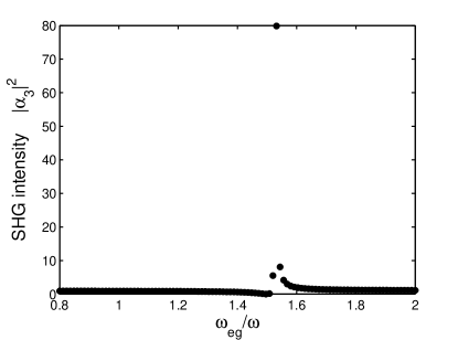
Figure 3: The enhancement of the FWM process. The FWM mode $\hat{a}_{3}$ is far-off resonant to the FWM condition $\left(\omega_{3}=1.85\omega\right)$. The FWM process can be carried closer to resonance by arranging the quantum level spacing to $\left(\omega_{eg}\approx 1.52\omega\right)$. The conversion is enhanced nearly $80$ times compared to off-resonant process. The conversion for off resonant process $\left(f=0\right)$ is represented by unity in figure. For $\left(\omega_{eg}=2\omega-\omega^{\prime}\right)$, FWM process is suppressed similar to Fig.1. Decay rates of the grating modes are taken as $\gamma_{1}=\gamma_{2}=\gamma_{3}=0.01\omega$. We use $\chi^{\left(2\right)}=0.00001\omega$ and $f=0.1\omega$ for numerical simulations.

III Two Coupled Quantum Dots

In case of two coupled QDs we have total Hamiltonian as Follows.

$$\hat{H}_{0}=\hbar\omega_{eg}^{(1)}\left|e_{1}\right\rangle\left\langle e_{1}\right|+\hbar\omega_{eg}^{(2)}\left|e_{2}\right\rangle\left\langle e_{2}\right|$$ (12)

$$\hat{H}_{grating}=\hbar\omega_{1}\hat{a}_{1}^{\dagger}\hat{a}_{1}+\hbar\omega_{2}\hat{a}_{2}^{\dagger}\hat{a}_{2}+\hbar\omega_{3}\hat{a}_{3}^{\dagger}\hat{a}_{3}$$ (13)

$$\hat{H}_{int}=\hbar\left[\left(f_{1}\hat{a}_{3}^{\dagger}\left|g_{1}\right\rangle\left\langle e_{1}\right|+f_{1}^{\ast}\hat{a}_{3}\left|e_{1}\right\rangle\left\langle g_{1}\right|\right)+\left(f_{2}\hat{a}_{3}^{\dagger}\left|g_{2}\right\rangle\left\langle e_{2}\right|+f_{2}^{\ast}\hat{a}_{3}\left|e_{2}\right\rangle\left\langle g_{2}\right|\right)\right]$$ (14)

Here, we have considered that level spacing of both the QDs is only resonant to $\hat{a}_{3}$ mode (i.e. $\omega_{eg}^{(1)}\sim\omega_{3}$, $\omega_{eg}^{(2)}\sim\omega_{3}$).

$$\hat{H}_{QE-QE}=\hbar\left[g\left(\left|e_{2}\right\rangle\left\langle g_{2}\right|\otimes\left|g_{1}\right\rangle\left\langle e_{1}\right|\right)+g^{\ast}\left(\left|e_{1}\right\rangle\left\langle g_{1}\right|\otimes\left|g_{2}\right\rangle\left\langle e_{2}\right|\right)\right]$$ (15)

as well as energy transferred by Pump Source with $e^{-i\omega t}$ and $e^{-i\omega^{\prime}t}$ respectively.

$$\hat{H}_{P}=i\hbar\left(\hat{a}_{1}^{\dagger}~{}\epsilon_{P}e^{-i\omega t}-\hat{a}_{1}~{}\epsilon_{P}^{\ast}e^{i\omega t}\right)+i\hbar\left(\hat{a}_{2}^{\dagger}~{}\epsilon_{P}^{\prime}e^{-i\omega^{\prime}t}-\hat{a}_{2}~{}\epsilon_{P}^{\ast\prime}e^{i\omega\prime t}\right)$$ (16)

$$\hat{H}_{FWM}=\hbar\chi^{(3)}\left(\hat{a}_{3}^{\dagger}\hat{a}_{2}^{\dagger}\hat{a}_{1}^{2}+\hat{a}_{1}^{\dagger 2}\hat{a}_{2}\hat{a}_{3}~{}\right)$$ (17)

is the Four Wave Mixing Hamiltonian for the Process of $\left(\omega_{3}=~{}2\omega_{1}-\omega_{2}\right)$ as mentioned in PRL 103, 266802.

By using the commutation relation Eq.(6) as well as proceeding like the same way for a single QD case, we get following equations for the case of coupled QDs.

$$\dot{\alpha}_{1}=\left(-i\omega_{1}-\gamma_{1}\right)\alpha_{1}-2i\chi^{\left(3\right)}\alpha_{1}^{\ast}\alpha_{2}\alpha_{3}+\epsilon_{p}e^{-i\omega t}$$ (18a)

$$\dot{\alpha}_{2}=\left(-i\omega_{2}-\gamma_{2}\right)\alpha_{2}-i\chi^{\left(3\right)}\alpha_{3}^{\ast}\alpha_{1}^{2}+\epsilon_{p}^{\prime}e^{-i\omega^{\prime}t}$$ (18b)

$$\dot{\alpha}_{3}=\left(-i\omega_{3}-\gamma_{3}\right)\alpha_{3}-i\chi^{\left(3\right)}\alpha_{2}^{\ast}\alpha_{1}^{2}-if_{1}\rho_{ge}^{\left(1\right)}-if_{2}\rho_{ge}^{\left(2\right)}$$ (18c)

$$\dot{\rho}_{ge}^{\left(1\right)}=\left(-i\omega_{eg}^{\left(1\right)}-\gamma_{eg}^{\left(1\right)}\right)\rho_{ge}^{\left(1\right)}+if_{1}^{\ast}\alpha_{3}\left(\rho_{ee}^{\left(1\right)}-\rho_{gg}^{\left(1\right)}\right)+ig^{\ast}\left(\rho_{ee}^{\left(1\right)}-\rho_{gg}^{\left(1\right)}\right)\rho_{ge}^{\left(2\right)}$$ (18d)

$$\dot{\rho}_{ge}^{\left(2\right)}=\left(-i\omega_{eg}^{\left(2\right)}-\gamma_{eg}^{\left(2\right)}\right)\rho_{ge}^{\left(2\right)}+if_{2}^{\ast}\alpha_{3}\left(\rho_{ee}^{\left(2\right)}-\rho_{gg}^{\left(2\right)}\right)+ig\left(\rho_{ee}^{\left(2\right)}-\rho_{gg}^{\left(2\right)}\right)\rho_{ge}^{\left(1\right)}$$ (18e)

$$\dot{\rho}_{ee}^{\left(1\right)}=-\gamma_{ee}^{\left(1\right)}\rho_{ee}^{\left(1\right)}+i\left(f_{1}\alpha_{3}^{\ast}\rho_{ge}^{\left(1\right)}-f_{1}^{\ast}\alpha_{3}\rho_{eg}^{\left(1\right)}\right)+i\left(g\rho_{eg}^{\left(2\right)}\rho_{ge}^{\left(1\right)}-g^{\ast}\rho_{eg}^{\left(1\right)}\rho_{ge}^{\left(2\right)}\right)$$ (18f)

$$\dot{\rho}_{ee}^{\left(2\right)}=-\gamma_{ee}^{\left(2\right)}\rho_{ee}^{\left(2\right)}+i\left(f_{2}\alpha_{3}^{\ast}\rho_{ge}^{\left(2\right)}-f_{2}^{\ast}\alpha_{3}\rho_{eg}^{\left(2\right)}\right)+i\left(g^{\ast}\rho_{eg}^{\left(1\right)}\rho_{ge}^{\left(2\right)}-g\rho_{eg}^{\left(2\right)}\rho_{ge}^{\left(1\right)}\right)$$ (18g)

where $\gamma_{1}$,$\gamma_{2},\gamma_{3}~{}$are the damping rates of the electromagnetic modes of the gold grating $\left(\alpha_{1},\alpha_{2},\alpha_{3}\right).~{}~{}\gamma_{ee}^{\left(1\right)}$, $\gamma_{ee}^{\left(2\right)}$ and $~{}\gamma_{eg}^{\left(1\right)}=\gamma_{ee}^{\left(1\right)}/2,~{}\gamma_{eg}^{\left(2\right)}=\gamma_{ee}^{\left(2\right)}/2,~{}$are the diagonal and off-diagonal decay rates of the first and second quantum emitter respectively. The constraints of the conservation probability $\rho_{ee}^{\left(1\right)}+~{}\rho_{gg}^{\left(1\right)}=1$ and $\rho_{ee}^{\left(2\right)}+~{}\rho_{gg}^{\left(2\right)}=1$ accompanies above set of Eqs.(18a-18g).

In our simulation for enhancement process of FWM, we time evolve Eqs. (18a-18g) numerically to obtain the long time behaviors of $\rho_{ge}^{\left(1\right)},\rho_{ge}^{\left(2\right)},\rho_{ee}^{\left(1\right)},\rho_{ee}^{\left(2\right)},\alpha_{1},\alpha_{2}~{}$ and $\alpha_{3}$. We determine the values to where they converge when the drive is on for long enough times. We perform this simulations for different parameter sets $\left(f_{1},f_{2},g,\omega_{eg}^{\left(1\right)},\omega_{eg}^{\left(2\right)},\gamma_{eg}^{\left(1\right)},\gamma_{eg}^{\left(2\right)}\right)$ with the initial condition $\rho_{ee}^{\left(1\right)}\left(t=0\right)=\rho_{ee}^{\left(2\right)}\left(t=0\right)=0,$ $\rho_{ge}^{\left(1\right)}\left(t=0\right)=\rho_{ge}^{\left(2\right)}\left(t=0\right)=0,~{}\alpha_{1}\left(0\right)=0,~{}\alpha_{2}\left(0\right)=0,~{}\alpha_{3}\left(0\right)=0$.

Besides the time-evolution simulations, one may gain the understanding by seeking the solutions of the following form:

$\alpha_{1}(t)=\tilde{\alpha}_{1}e^{-i\omega t}$, $\alpha_{2}(t)=\tilde{\alpha}_{2}e^{-i\omega^{\prime}t}$, $\alpha_{3}(t)=\tilde{\alpha}_{3}e^{-i\left(2\omega-\omega^{\prime}\right)t}$ (Condition of Four wave mixing process), $\rho_{ge}^{\left(1\right)}=\tilde{\rho}_{ge}^{\left(1\right)}e^{-i\left(2\omega-\omega^{\prime}\right)t}$, $\rho_{ge}^{\left(2\right)}=\tilde{\rho}_{ge}^{\left(2\right)}e^{-i\left(2\omega-\omega^{\prime}\right)t}$.

Here we have considered that level spacing of both the QDs is only resonant to $\hat{a}_{3}$ mode (i.e. $\omega_{eg}^{\left(1\right)}\sim\omega_{3},\omega_{eg}^{\left(2\right)}\sim\omega_{3})$, $\rho_{ee}^{\left(1\right)}(t)=\tilde{\rho}_{ee}^{\left(1\right)}~{}$ and $\rho_{ee}^{\left(2\right)}(t)=\tilde{\rho}_{ee}^{\left(2\right)}$.
Inserting the solutions in above set of Eqs. (18a-18g) we have the following closed set of equations for the steady state dynamics

$$\left[i\left(\omega_{1}-\omega\right)+\gamma_{1}\right]\tilde{\alpha}_{1}+2i\chi^{\left(3\right)}\tilde{\alpha}_{1}^{\ast}\tilde{\alpha}_{2}\tilde{\alpha}_{3}=\epsilon_{p}$$ (19a)

$$\left[i\left(\omega_{2}-\omega^{\prime}\right)+\gamma_{2}\right]\tilde{\alpha}_{2}+i\chi^{\left(3\right)}\tilde{\alpha}_{3}^{\ast}\tilde{\alpha}_{1}^{2}=\epsilon_{p}^{\prime}$$ (19b)

$$\left[i\left(\omega_{3}+\omega^{\prime}-2\omega\right)+\gamma_{3}\right]\tilde{\alpha}_{3}+i\chi^{\left(3\right)}\tilde{\alpha}_{2}^{\ast}\tilde{\alpha}_{1}^{2}=-if_{1}\tilde{\rho}_{ge}^{\left(1\right)}--if_{2}\tilde{\rho}_{ge}^{\left(2\right)}$$ (19c)

$$\left[i\left(\omega_{eg}^{\left(1\right)}+\omega^{\prime}-2\omega\right)+\gamma_{eg}^{\left(1\right)}\right]\tilde{\rho}_{ge}^{\left(1\right)}=if_{1}^{\ast}\tilde{\alpha}_{3}y_{1}+ig^{\ast}y_{1}\tilde{\rho}_{ge}^{\left(2\right)}$$ (19d)

$$\left[i\left(\omega_{eg}^{\left(2\right)}+\omega^{\prime}-2\omega\right)+\gamma_{eg}^{\left(2\right)}\right]\tilde{\rho}_{ge}^{\left(2\right)}=if_{2}^{\ast}\tilde{\alpha}_{3}y_{2}+igy_{2}\tilde{\rho}_{ge}^{\left(1\right)}$$ (19e)

$$\gamma_{ee}^{\left(1\right)}\tilde{\rho}_{ee}^{\left(1\right)}=i\left(f_{1}\tilde{\alpha}_{3}^{\ast}\tilde{\rho}_{ge}^{\left(1\right)}-f_{1}^{\ast}\tilde{\alpha}_{3}\tilde{\rho}_{eg}^{\left(1\right)}\right)+i\left(g\tilde{\rho}_{eg}^{\left(2\right)}\tilde{\rho}_{ge}^{\left(1\right)}-g^{\ast}\tilde{\rho}_{eg}^{\left(1\right)}\tilde{\rho}_{ge}^{\left(2\right)}\right)$$ (19f)

$$\gamma_{ee}^{\left(2\right)}\tilde{\rho}_{ee}^{\left(2\right)}=i\left(f_{2}\tilde{\alpha}_{3}^{\ast}\tilde{\rho}_{ge}^{\left(2\right)}-f_{2}^{\ast}\tilde{\alpha}_{3}\tilde{\rho}_{eg}^{\left(2\right)}\right)+i\left(g^{\ast}\tilde{\rho}_{eg}^{\left(1\right)}\tilde{\rho}_{ge}^{\left(2\right)}-g\tilde{\rho}_{eg}^{\left(2\right)}\tilde{\rho}_{ge}^{\left(1\right)}\right)$$ (19g)

where $$\tilde{\alpha}_{1},\tilde{\alpha}_{2},\tilde{\alpha}_{3},\tilde{\rho}_{ge}^{\left(1\right)},\tilde{\rho}_{ge}^{\left(2\right)},\tilde{\rho}_{ee}^{\left(1\right)} \tilde{\rho}_{ee}^{\left(2\right)} y_{i}=\left(\tilde{\rho}_{ee}^{\left(i\right)}-\tilde{\rho}_{gg}^{\left(i\right)}\right)~{} \left(i=1,2\right)$$ and are constants independent of time. are the population inversion for both QDs.

Using Eqs.(19d) and (19e) in Eq.(19c), we obtain the steady state value for $\tilde{\alpha}_{3}$ as follows.

$$\tilde{\alpha}_{3}=\frac{i\chi^{\left(3\right)}\left(\beta_{1}\beta_{2}+y_{1}y_{2}\left|g\right|^{2}\right)}{\left(y_{1}\left|f_{1}\right|^{2}\beta_{2}+y_{2}\left|f_{2}\right|^{2}\beta_{1}\right)+iy_{1}y_{2}\left(f_{1}f_{2}^{\ast}g^{\ast}+f_{1}^{\ast}f_{2}g\right)-\varepsilon_{3}\left(\beta_{1}\beta_{2}+y_{1}y_{2}\left|g\right|^{2}\right)}\tilde{\alpha}_{2}^{\ast}\tilde{\alpha}_{1}^{2}$$ (20)

where the short hand notations are $\varepsilon_{1}=\left[i\left(\omega_{1}-\omega\right)+\gamma_{1}\right],~{}\varepsilon_{2}=\left[i\left(\omega_{2}-\omega^{\prime}\right)+\gamma_{2}\right],~{}\varepsilon_{3}=\left[i\left(\omega_{3}+\omega^{\prime}-2\omega\right)+\gamma_{3}\right]~{}$ and $\beta_{1}=\left[i\left(\omega_{eg}^{\left(1\right)}+\omega^{\prime}-2\omega\right)+\gamma_{eg}^{\left(1\right)}\right]~{}$ and $\beta_{2}=\left[i\left(\omega_{eg}^{\left(2\right)}+\omega^{\prime}-2\omega\right)+\gamma_{eg}^{\left(2\right)}\right].$

III.1 Super enhancement of FWM process

III.1.1 Single QD case

In case of a single QD coupled to the gold grating, $f_{2}=g=g^{\ast}=0$ and $f_{1}=f$, we get the steady state value of $\tilde{\alpha}_{3}\$ from Eq.(20)as

$$\tilde{\alpha}_{3}=\frac{i\chi^{\left(3\right)}\tilde{\alpha}_{2}^{\ast}\tilde{\alpha}_{1}^{2}}{\frac{\left|f\right|^{2}y}{\left[i\left(\omega_{eg}+\omega^{\prime}-2\omega\right)+\gamma_{eg}\right]}-\left[i\left(\omega_{3}+\omega^{\prime}-2\omega\right)+\gamma_{3}\right]}$$ (21)

which coincides exactly with Eq.(9) where the imaginary part of the first term $\frac{\left|f\right|^{2}y}{\left[i\left(\omega_{eg}+\omega^{\prime}-2\omega\right)+\gamma_{eg}\right]}$ can be arranged to cancel the $i\left(\omega_{3}+\omega^{\prime}-2\omega\right)$ factor in the second term of the denominator and this gives enhancement of FWM as also discussed in previous section also.

III.1.2 Coupled QDs case

As compared to single QD case, the denominator of Eq.(20) can (in principal) be arranged down to very low values in order to enhance $\tilde{\alpha}_{3}$ to much higher values. In this case, denominator has 3 complex $\left(f_{1},f_{2},g\right)$ and 2 real $\left(\omega_{eg}^{\left(1\right)},\omega_{eg}^{\left(2\right)}\right)$ parameters which can be tuned independently.

We obtain nearly $1200$ times enhancement by comparing the steady state values of $\left|\tilde{\alpha}_{3}\right|^{2}$ that is the intensity of FWM process calculated from time evolution of Eqs.$\left(18a-18g\right)$ for the chosen set of parameters as shown in Fig.$\left(4\right)$. Here, frequency of second QD is kept constant and first one is varying. For the decay rates of grating modes in between $0.01$, we get enhancement in FWM Intensity around 1200-1600 times as compared to case of single QD discussed in previous section.

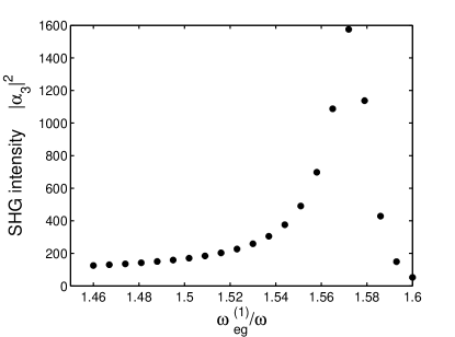
Figure 4: The enhancement of the FWM process in case of coupled QDs. The FWM mode $\hat{a}_{3}$ is far-off resonant to the FWM condition $\left(\omega_{3}=1.90\omega\right)$. The FWM process can be carried closer to resonance by arranging the quantum level spacing of first QD to $\left(\omega_{eg}^{\left(1\right)}\approx 1.5732\omega\right)$, while second QD $\left(\omega_{eg}^{\left(2\right)}=1.5810\omega\right)$ being fixed . The conversion is enhanced nearly by $1600$ times. Decay rates of the grating modes are taken as $\gamma_{1}=\gamma_{2}=\gamma_{3}=0.01\omega$. We use $\chi^{\left(2\right)}=0.00001\omega$ and $f_{1}=f_{2}=0.1909\omega$, $g=\left(0.1000+0.0101i\right)\omega$,$\gamma_{ee}^{\left(1\right)}=\gamma_{ee}^{\left(2\right)}=0.00001\omega$, $\gamma_{eg}^{\left(1\right)}=\gamma_{ee}^{\left(1\right)}/2$, $\gamma_{eg}^{\left(2\right)}=\gamma_{ee}^{\left(2\right)}/2$ for our numerical simulations.

IV conclusion

It is well demonstrated that the presence of a quantum emitter with a smaller decay rate changes the optical response of coupled grating dramatically. Due to the destructive interference of the (hybridized) absorption paths, Four wave mixing(FWM) process can be suppressed at the resonance frequency of the quantum emitter. We demonstrate that a similar path interference effect can be adopted to both suppress and enhance the nonlinear Four wave mixing processes (FWM) in a grating surface. A quantum emitter is coupled with the electromagnetic modes of a gold grating. We found that the FWM process can be suppressed over 10 orders of magnitude. Such an suppression can be achieved by carefully choosing the coupling strengths and the energy level spacing for quantum emitters. When $\left(\omega_{eg}=2\omega-\omega^{\prime}\right)$, the FWM intensity can be suppressed by several order of magnitude with respect to resonant value. On the other hand, the similar interference effects can be also used to enhance the nonlinear FWM intensity. The level spacing of the single quantum emitter can be arranged so that the nonresonant terms get canceled. In case of two coupled quantum emitters by arranging energy level spacing for quantum emitters in the same way like single quantum emitter, we have enhancement in FWM intensity upto the order of $10^{3}$.

References

(1) M.S.Tame; M.S. Kim, Nature Physics 9, 329-340 (2013).
(2) Z. Lu; K. D. Zhu, J. Phys. B. 42, 0155502 (2009).
(3) A. Hatef; M.R. Singh, Phys. Rev. A. 81, 063816 (2010).