Bayesian Nonparametric Modeling of Higher Order Markov Chains

Abstract

We consider the problem of flexible modeling of higher order Markov chains when an upper bound on the order of the chain is known but the true order and nature of the serial dependence are unknown. We propose Bayesian nonparametric methodology based on conditional tensor factorizations, which can characterize any transition probability with a specified maximal order. The methodology selects the important lags and captures higher order interactions among the lags, while also facilitating calculation of Bayes factors for a variety of hypotheses of interest. We design efficient Markov chain Monte Carlo algorithms for posterior computation, allowing for uncertainty in the set of important lags to be included and in the nature and order of the serial dependence. The methods are illustrated using simulation experiments and real world applications.

Some Key Words: Bayesian nonparametrics, Categorical time series, Conditional tensor factorization, Higher order Markov chains, Sequential categorical data.

Short Title: Higher Order Markov Chains

1 Introduction

For $t=1,\ldots,T$, consider a time indexed sequence of categorical variables $\{y_{t}\}$. We assume that the distribution of $y_{t}$ may depend on the values at the previous $q$ time points, $y_{t-1},\ldots,y_{t-q}$. For $t=(q+1),\dots,T$, the transition probability law governing the evolution of the sequence satisfies

$$p(y_{t}\mid y_{t-1},\dots,y_{1})=p(y_{t}\mid y_{t-1},\dots,y_{t-q}),$$

and the likelihood function of the sequence admits the factorization

$$p({\mathbf{y}}_{1:T})=p_{0}({\mathbf{y}}_{1:q})\prod_{t=(q+1)}^{T}p(y_{t}\mid y_{t-1},\dots,y_{t-q}),$$

where $p_{0}$ denotes the distribution of the initial $q$ variables ${\mathbf{y}}_{1:q}$; we follow common convention and condition on the initial observations to avoid modeling $p_{0}$.

We call such a sequence a Markov chain of maximal order $q$ if conditional on the values of $(y_{t-1},\dots,y_{t-q})$, the distribution of $y_{t}$ is independent of its more distant past, but the actual lags important in determining the distribution of $y_{t}$ may be an arbitrary subset of $(y_{t-1},\ldots,y_{t-q})$. In contrast, if the distribution of $y_{t}$ actually varies with the values at all the previous $q$ times points, we call the sequence a Markov chain of full order $q$. The case $q=0$ corresponds to serial independence.

For a chain with $C_{0}$ states, there are $C_{0}-1$ free parameters in the conditional distribution of $y_{t}$, which can potentially vary arbitrarily with every possible combination of the levels of the previous variables. For a Markov chain of maximal order $q$, there are a total of $C_{0}^{q}$ such combinations, and hence the number of parameters in the full model is $(C_{0}-1)C_{0}^{q}$. This number increases exponentially in the order of the chain, creating estimation problems as $q$ increases. It is very important to define flexible, parsimonious and interpretable representations, with unnecessary lags eliminated.

A common approach to modeling higher order Markov chains is based on multinomial logit or probit models, with the lags included as linear predictors (Liang and Zeger, 1986; Zeger and Liang, 1986). Modeling $r^{th}$ order interactions among the lags using such models would require the inclusion of ${q\choose r}(C_{0}-1)^{r}$ interaction terms in the set of linear predictors. The number of interaction terms thus increases rapidly with $C_{0}$ and $q$. For example, with only $5$ lags and $4$ categories, accommodation of second order interactions requires the inclusion of $90$ interaction terms. In practical applications, attention is thus often restricted to only a small number of lags and low order interaction terms (Fahrmier and Kaufmann, 1987).

An alternative that can accommodate a relatively large number of lags but ignores interactions among lags is mixtures of transition distributions (MTD). In the basic MTD model (Raftery, 1985a), the transition probability $p(y_{t}\mid y_{t-1},\dots,y_{t-q})$ is a linear combination of $Q(y_{t-1},y_{t}),\dots,Q(y_{t-q},y_{t})$, where $Q$ is a $C_{0}\times C_{0}$ transition matrix for a first order Markov chain. Raftery (1985b) and Berchtold (1995, 1996) allowed different transition matrices for different lags. Raftery and Tavaré (1994) and Berchtold and Raftery (2002) discussed estimation algorithms and other generalizations. While MTD leads to parsimonious models for higher order Markov chains, it is not structurally rich, particularly when size of the state space and/or the order of the chain is large. Additionally, the model implicitly assumes the process is of full order $q$, with selection of $q$ requiring refitting for different choices.

Another popular strategy to modeling higher order Markov chains is based on trees with conditioning sequences of different lengths as nodes and leaves. Variable length Markov chains (VLMC) (Bühlmann and Wyner, 1999; Ron et al., 1996) prune large branches, keeping only those nodes whose effects on $y_{t}$ are different enough from their parent’s. Context tree weighting (Willems et al., 1995) uses an ensemble of trees of varying depths. The sequence memoizer (Teh, 2006; Wood et al., 2011) uses a hierarchical prior to center the children $p(y_{t}\mid y_{t-1},\dots,y_{t-r})$ around their parent $p(y_{t}\mid y_{t-1},\dots,y_{t-(r-1)})$ for each $r\geq 1$, which favors a restrictive structure. In general, tree based methods are not suitable when a more distant lag may be a more important predictor of $y_{t}$ than a relatively recent one. Sparse Markov chains (SMC) (Jääskinen et al., 2014) attempt to remove this limitation. SMCs cluster the lag combinations having similar influence on the transition distribution of $y_{t}$, related to VLMC but leaving the partitioning unrestricted. Such hard clustering may lead to oversimplification of the dependence structure for long sequences. Additionally, hard clustering and tree based approaches do not explicitly characterize significance of individual lags or provide a framework for testing of related hypotheses.

In this article, we take a fundamentally different approach. Tensor factorizations for categorical regression have been developed in Yang and Dunson (2015). We adapt these factorizations to our dynamic setting, while incorporating substantial improvements to the structure and computation. The proposed formulation leads to parsimonious representations of transition probability tensors, shrinking towards low dimensional structures and borrowing strength across lags, while being flexible in capturing complex higher order interactions. The method allows automated order and lag selection, quantifying uncertainty in selection and facilitating testing of hypotheses. Convergence of the posterior to the true transition probability tensor is guaranteed under ergodicity of the true data generating process. Taking a novel approach to posterior computation in variable dimension models, we develop an efficient Markov chain Monte Carlo (MCMC) algorithm.

The article is organized as follows. Section 2 details our model and its interesting aspects. Section 3 describes MCMC algorithms to sample from the posterior. Section 4 presents the results of simulation experiments comparing our method with existing approaches. Section 5 presents some applications of the proposed method. Section 6 contains concluding remarks.

2 Model Specification

2.1 Review of Tensor Factorizations

There is a vast literature on tensor factorizations, the two most popular approaches being parallel factor analysis (PARAFAC) and higher order singular value decomposition (HOSVD). PARAFAC (Harshman, 1970) decomposes a $D_{1}\times\dots\times D_{p}$ dimensional tensor ${\mathbf{M}}=\{m_{x_{1},\dots,x_{p}}\}$ as the sum of rank one tensors as

$$m_{x_{1},\dots,x_{p}}=\sum_{h=1}^{k}g_{h}\prod_{j=1}^{p}u_{h}^{(j)}(x_{j}).$$ (1)

In contrast, HOSVD, proposed by Tucker (1966) for three way tensors and extended to the general case by De Lathauwer et al. (2000), factorizes ${\mathbf{M}}$ as

$$m_{x_{1},\dots,x_{p}}=\sum_{h_{1}=1}^{k_{1}}\cdots\sum_{h_{p}=1}^{k_{p}}g_{h_{1},\dots,h_{p}}\prod_{j=1}^{p}u_{h_{j}}^{(j)}(x_{j}),$$ (2)

where ${\mathbf{G}}=\{g_{h_{1},\dots,h_{p}}\}$, called a core tensor, captures interactions between the different components and ${\mathbf{U}}_{j}=\{u_{h_{j}}^{(j)}(x_{j})\}$ are component specific weights. See Figure 1. HOSVD achieves better data compression and requires fewer components compared to PARAFAC, which can be obtained as a special case of HOSVD with ${\mathbf{G}}$ diagonal.

Figure 1: Pictorial representation of HOSVD for a 3 way tensor ${\mathbf{M}}$ with core tensor ${\mathbf{G}}$ and weight matrices ${\mathbf{U}}_{j},j=1,2,3$.

The tensor factorization that is most relevant to our problem was introduced in Yang and Dunson (2015) (YD). YD considered the problem of regressing a categorical response variable $y\in\{1,\dots,D_{0}\}$ on categorical predictors $x_{j}\in\{1,\dots,D_{j}\}$, $j=1,\dots,p$. Structuring the conditional probabilities $p(y\mid x_{j},j=1,\dots,p)$ as the elements of a $D_{0}\times D_{1}\times\dots\times D_{p}$ dimensional tensor, YD proposed the following HOSVD-type factorization

$$p(y\mid x_{j},j=1,\dots,p)=\sum_{h_{1}=1}^{k_{1}}\cdots\sum_{h_{p}=1}^{k_{p}}\lambda_{h_{1}\dots h_{p}}(y)\prod_{j=1}^{p}\pi_{h_{j}}^{(j)}(x_{j}),$$ (3)

where $1\leq k_{j}\leq D_{j}$ for $j=1,\dots,p$ and the parameters $\lambda_{h_{1},\dots,h_{p}}(y)$ and $\pi_{h_{j}}^{(j)}(x_{j})$ are all non-negative and satisfy the constraints (a) $\sum_{y=1}^{D_{0}}\lambda_{h_{1}\dots h_{p}}(y)=1$ for each combination $(h_{1},\dots,h_{p})$, and (b) $\sum_{h_{j}=1}^{k_{j}}\pi_{h_{j}}^{(j)}(x_{j})=1$ for each pair $(j,x_{j})$. They established that any conditional probability tensor can be represented as (3), with the parameters satisfying the constraints (a) and (b). The constraints (a) and (b) are thus not restrictive but they ensure that $\sum_{y=1}^{D_{0}}p(y\mid x_{j},j=1,\dots,p)=1$.

Taking a Bayesian approach, they assigned sparsity inducing priors on the $k_{j}$’s and conditional on the $k_{j}$’s, placed independent Dirichlet priors on $\lambda_{h_{1},\dots,h_{p}}(y)$’s and $\pi_{h_{j}}^{(j)}(x_{j})$’s as $\{\lambda_{h_{1},\dots,h_{q}}(1),\dots,\lambda_{h_{1},\dots,h_{p}}(D_{0})\}\sim\hbox{Dir}(1/D_{0},\dots,1/D_{0})$ for each combination $(h_{1},\dots,h_{p})$ with $1\leq h_{j}\leq k_{j}$ and $\{\pi_{1}^{(j)}(x_{j}),\dots,\pi_{k_{j}}^{(j)}(x_{j})\}\sim\hbox{Dir}(1/k_{j},\dots,1/k_{j})$ for each $x_{j}\in\{1,\dots,D_{j}\}$. The dimensions of these parameters vary with $k_{j}$’s, making the design of efficient MCMC algorithms challenging. YD used an approximate two-stage sampler, selecting the $k_{j}$’s in the first stage and then sampling the other parameters in the second stage while keeping the $k_{j}$’s fixed.

2.2 Higher Order Markov Chains via Tensor Factorization

We propose a nonparametric Bayes approach for inferring the order and structure of higher order Markov chains building on a YD-type conditional tensor factorization. In our dynamic setting, we have a time-indexed categorical sequence $\{y_{t}\}$ with finite memory of maximal order $q$ taking values in the set $\{1,\dots,C_{0}\}$. Given $y_{t-1},\ldots,y_{t-q}$, the distribution of $y_{t}$ is independent of all observations prior to $t-q$. The variables that are important in predicting $y_{t}$ can potentially constitute a subset of $\{y_{t-1},\ldots,y_{t-q}\}$. For $t=q+1,\dots,T$, the transition probability $p(y_{t}\mid y_{t-1},\ldots,y_{t-q})$ is structured as a $C_{0}\times C_{0}\times\dots\times C_{0}$ dimensional tensor and admits the factorization

$$p(y_{t}\mid y_{t-j},j=1,\dots,q)=\sum_{h_{1}=1}^{k_{1}}\cdots\sum_{h_{q}=1}^{k_{q}}\lambda_{h_{1},\dots,h_{q}}(y_{t})\prod_{j=1}^{q}\pi_{h_{j}}^{(j)}(y_{t-j}),$$ (4)

where, with some repetition, $1\leq k_{j}\leq C_{0}$ for all $j$ and the parameters $\lambda_{h_{1},\dots,h_{p}}(y_{t})$ and $\pi_{h_{j}}^{(j)}(y_{t-j})$ are all non-negative and satisfy the constraints

$$\sum_{y_{t}=1}^{C_{0}}\lambda_{h_{1},\dots,h_{q}}(y_{t})=1,~{}~{}\text{for each combination}~{}(h_{1},\dots,h_{q}),$$ (5)

$$\sum_{h_{j}=1}^{k_{j}}\pi_{h_{j}}^{(j)}(y_{t-j})=1,~{}~{}\text{for each pair }~{}(j,y_{t-j}).$$ (6)

Introducing latent allocation variables $z_{j,t}$ for each $j=1,\dots,q$ and $t=q+1,\dots,T$, the response values are conditionally independent and the factorization can be equivalently represented through the following hierarchical formulation:

$$(y_{t}\mid z_{j,t}=h_{j},j=1,\dots,q) \sim \hbox{Mult}(\{1,\dots,C_{0}\},\lambda_{h_{1},\dots,h_{q}}(1),\dots,\lambda_{h_{1},\dots,h_{q}}(C_{0})),$$ (7)

$$(z_{j,t}\mid y_{t-j}) \sim \hbox{Mult}(\{1,\dots,k_{j}\},\pi_{1}^{(j)}(y_{t-j}),\dots\pi_{k_{j}}^{(j)}(y_{t-j})).$$ (8)

See Figure 2. Posterior computation is facilitated by sampling these latent auxiliary variables. This formulation also aids in understanding interesting features of the model. Equation (8), for instance, reveals the soft clustering property of the model that enables it to borrow strength across the different categories of $y_{t-j}$ by allowing the $z_{j,t}$’s associated with a particular state of $y_{t-j}$ to be allocated to different latent populations, which are shared across all $C_{0}$ states of $y_{t-j}$. Equation (7), on the other hand, shows how such soft assignment enables the model to capture complex interactions among the lags in an implicit and parsimonious manner by allowing the latent populations indexed by $(h_{1},\dots,h_{q})$ to be shared among the various state combinations of the lags.

(a)

(b)

Figure 2: Graphical model depicting the dependence structure of a second order Markov chain $\{y_{t}\}$ (a) without and (b) with latent variables $\{z_{j,t}\}$.

When $k_{j}=1$, $\pi_{1}^{(j)}(y_{t-j})=1$ and $p(y_{t}\mid y_{t-1},\ldots,y_{t-q})$ does not vary with $y_{t-j}$. The variable $k_{j}$ thus determines the inclusion of the $j^{th}$ lag $y_{t-j}$ in the model. The variable $k_{j}$ also determines the number of latent classes for the $j^{th}$ lag $y_{t-j}$. The number of parameters in such a factorization is given by $(C_{0}-1)\prod_{j=1}^{q}k_{j}+C_{0}\sum_{j=1}^{q}(k_{j}-1)$, which will be much smaller than the number of parameters $(C_{0}-1)C_{0}^{q}$ required to specify a full Markov model of the same maximal order if $\prod_{j=1}^{q}k_{j}\ll C_{0}^{q}$.

In practical applications $\prod_{j=1}^{q}k_{j}$ may still be quite large. For instance, for a Markov chain with $C_{0}=4$ states and $5$ important lags with $k_{j}=3$ for all $j=1,\dots,5$, the number of parameters required to specify the core tensor will be $3\times 3^{5}=729$. While this results in a significant reduction in the number of parameters compared to a fully specified Markov model of the same maximal order which requires $3\times 4^{5}=3072$ parameters, it may still be too large for efficient and numerically stable estimation of the parameters for data sets of sizes that are typically encountered in practice.

Towards a more parsimonious representation, we note that the conditional tensor factorization (4) can be interpreted as a predictor dependent mixture model for modeling distributions supported on $\{1,\dots,C_{0}\}$. Here the probability vectors $\mbox{\boldmath$\lambda$}_{h_{1},\dots,h_{q}}=\{\lambda_{h_{1},\dots,h_{q}}(1),\dots,\lambda_{h_{1},\dots,h_{p}}(C_{0})\}$ that constitute the core tensor play the role of kernels of the mixture model, and $\pi_{h_{1},\dots,h_{q}}(y_{t-1},\dots,y_{t-q})=\prod_{j=1}^{q}\pi_{h_{j}}^{(j)}(y_{t-j})$ play the role of associated predictor dependent mixture weights. Given $k_{1},\dots,k_{q}$, the kernels are indexed by $(h_{1},\dots,h_{q})$ with $h_{j}=1,\dots,k_{j}$, contributing $\prod_{j=1}^{q}k_{j}$ mixture components to the model. Thus, the number of kernels determines the effective dimension of the model. In most applications, a very large number of kernels may not be required. This is especially true for discrete distributions supported on a finite set $\{1,\dots,C_{0}\}$.

A more parsimonious representation that retains the flexibility of the original model is obtained by encouraging the kernels $\mbox{\boldmath$\lambda$}_{h_{1},\dots,h_{q}}$ to be shared amongst the label combinations $(h_{1},\dots,h_{q})$ through probabilistic clustering. Specifically, we let

$$\mbox{\boldmath$\lambda$}_{h_{1},\dots,h_{q}} \sim \sum_{\ell=1}^{\infty}\pi_{\ell}^{\star}\delta_{\mbox{\boldmath$\lambda$}_{\ell}^{\star}},~{}~{}\hbox{independently for each}~{}(h_{1},\dots,h_{q}),$$ (9)

$$\mbox{\boldmath$\lambda$}_{\ell}^{\star}=\{\lambda_{\ell}^{\star}(1),\dots,\lambda_{\ell}^{\star}(C_{0})\} \sim \hbox{Dir}(\alpha,\dots,\alpha),~{}~{}\hbox{independently for}~{}\ell=1,\dots,\infty,~{}$$ (10)

$$\pi_{\ell}^{\star}=V_{\ell}\prod_{m=1}^{\ell-1}(1-V_{m}),~{}~{}~{}~{}~{}V_{\ell} \sim \hbox{Beta}(1,\alpha_{0}),~{}~{}\hbox{independently for}~{}\ell=1,\dots,\infty.$$ (11)

Introducing latent variables $z_{t}^{\star}$ and $z_{h_{1},\dots,h_{q}}^{\star}$, for $t=t^{\star},\dots,T$, $h_{j}=1,\dots,k_{j}$, $j=1,\dots,q$, we further have

$$p(z_{h_{1},\dots,h_{q}}^{\star}=\ell)~{}=~{}\pi_{\ell}^{\star},~{}~{}\hbox{independently for each}~{}(h_{1},\dots,h_{q}),$$ (12)

$$(\mbox{\boldmath$\lambda$}_{h_{1},\dots,h_{q}}\mid z_{h_{1},\dots,h_{q}}^{\star}=\ell)~{}=~{}\mbox{\boldmath$\lambda$}_{\ell}^{\star},~{}~{}~{}~{}~{}~{}(z_{t}^{\star}\mid z_{j,t}=h_{j},j=1,\dots,q)=z_{h_{1},\dots,h_{q}}^{\star},$$ (13)

$$(y_{t}\mid z_{t}^{\star}=\ell)~{}\sim~{}\hbox{Mult}(\{1,\dots,C_{0}\},\lambda_{\ell}^{\star}(1),\dots,\lambda_{\ell}^{\star}(C_{0})).$$ (14)

See Figure 3. The cluster inducing prior specified through (9)-(11) corresponds to a Dirichlet process (DP) prior (Ferguson, 1973) written in terms of its stick-breaking representation (Sethuraman, 1994). Although the prior allows infinitely many components, the number of components occupied by the $\prod_{j=1}^{q}k_{j}$ mixture kernels is finite and likely much smaller than $\prod_{j=1}^{q}k_{j}$, leading to a significant reduction in the effective number of parameters of the model. Our experiments suggest that, even in low to moderate dimensional problems, such clustering of kernels greatly improves numerical stability compared with assigning continuous priors on the kernels. The idea of hierarchical sharing of the kernels constituting the core tensor is not specific to our dynamic setting, and can be easily adapted to other tensor factorization models including the original YD model, also eliminating problems with exceeding limited storage space that plague YD in applications we have considered.

Figure 3: Graphical model depicting the dependence structure of a second order Markov chain $\{y_{t}\}$ with latent variables $\{z_{j,t}\}$ and $\{z_{t}^{\star}\}$.

The DP prior on the mixture kernels $\mbox{\boldmath$\lambda$}_{h_{1},\dots,h_{q}}$ treats the kernel indices $(h_{1},\dots,h_{q})$ as exchangeable. Although it is conceptually appealing to favor clustering of kernels with similar indices $(h_{1},\dots,h_{q})$, there is an associated significant increase in model complexity and computational costs. Hence, given that exchangeable priors worked well in examples we considered, we did not consider such modifications further. Although we focused on a DP prior for simplicity, other exchangeable clustering priors, such as Pitman-Yor processes (Pitman and Yor, 1997) or probit stick-breaking processes (Rodriguez and Dunson, 2011), can be used.

Next, consider mixture probability vectors $\mbox{\boldmath$\pi$}_{k_{j}}^{(j)}(y_{t-j})=\{\pi_{1}^{(j)}(y_{t-j}),\dots,\pi_{k_{j}}^{(j)}(y_{t-j})\}$. The dimension of $\mbox{\boldmath$\pi$}_{k_{j}}^{(j)}(y_{t-j})$, unlike the $\mbox{\boldmath$\lambda$}_{h_{1},\dots,h_{q}}$’s, varies linearly with $k_{j}$. For a Markov chain with $y_{0}=4$ states and $5$ important lags with $k_{j}=3$ for all $j=1,\dots,5$, the number of parameters contributed by all the $\mbox{\boldmath$\pi$}_{k_{j}}^{(j)}(y_{t-j})$ vectors will only be $4\times 2\times 5=40$. We thus assign independent priors on $\mbox{\boldmath$\pi$}_{k_{j}}(y_{t-j})$ as

$$\mbox{\boldmath$\pi$}_{k_{j}}^{(j)}(y_{t-j})=\{\pi_{1}^{(j)}(y_{t-j}),\dots,\pi_{k_{j}}^{(j)}(y_{t-j})\} \sim \hbox{Dir}(\gamma_{j},\dots,\gamma_{j}).$$ (15)

The probability vectors $\mbox{\boldmath$\pi$}_{k_{j}}^{(j)}(y_{t-j})$ are supported on $\{1,\dots,k_{j}\}$ for each pair $(j,y_{t-j})$. Therefore, unlike for $\mbox{\boldmath$\lambda$}_{h_{1},\dots,h_{q}}$, conditioning on $k_{j}$, which we have kept implicit in (15), can not be avoided. We, however, do not allow the hyper-parameter $\gamma_{j}$ to vary with $k_{j}$. This has important consequences in the design of our MCMC sampler. Details are deferred to Section 3.1.

Finally, model specification is completed by assigning priors on ${\mathbf{k}}$. We assign independent priors on $k_{j}$’s as

$$p(k_{j}=k) = p_{0,j}(k)~{}\propto~{}\exp(-\varphi jk),~{}~{}~{}j=1,\dots,q,~{}k=1,\dots,C_{0},$$ (16)

where $\varphi>0$. The prior assigns increasing probabilities to smaller values of $k_{j}$ as the lag $j$ becomes more distant, reflecting the natural belief that increasing lags will have diminishing influence on the distribution of $y_{t}$. Larger values of $\varphi$ imply faster decay of $p_{0,j}(k)$ with increase in $j$ and $k$, favoring sparser models. See Figure S.1 in the Supplementary Materials. The model space can be restricted to the class of Markov models of full order by restricting the prior to satisfy the condition that $k_{j+1}=1$ whenever $k_{j}=1$ for some $j$. It is appealing to avoid such restrictions to accommodate scenarios where a more distant lag is an important predictor of $y_{t}$ but a lag in the more recent past is not. As illustrated in Section 5, such scenarios are often encountered in practice.

Let ${\mathbf{y}}=\{y_{t}:t=t^{\star},\dots,T\}$, ${\mathbf{z}}=\{z_{j,t}:t=t^{\star},\dots,T,j=1,\dots,q\}$ and ${\mathbf{z}}^{\star}=\{z_{h_{1},\dots,h_{q}}^{\star}:h_{j}=1,\dots,k_{j},j=1,\dots,q\}$, where $t^{\star}=(q+1)$. Collecting all potential predictors of $y_{t}$ in ${\mathbf{w}}_{t}=(w_{1,t},\ldots,w_{q,t})^{\rm T}$ with $w_{j,t}=y_{t-j}$ for $j=1,\ldots,q$ and $t=t^{\star},\dots,T$, the joint distribution of ${\mathbf{y}}$, ${\mathbf{z}}$ and ${\mathbf{z}}^{\star}$ admits the factorization

$$p({\mathbf{y}},{\mathbf{z}},{\mathbf{z}}^{\star}\mid\mbox{\boldmath$\lambda$}^{\star},\mbox{\boldmath$\pi$}^{\star},\mbox{\boldmath$\pi$}_{{\mathbf{k}}},{\mathbf{k}})=\prod_{t=t^{\star}}^{T}\left\{p(y_{t}\mid\mbox{\boldmath$\lambda$}_{z_{{\mathbf{z}}_{t}}^{\star}}^{\star})\prod_{j=1}^{q}p(z_{j,t}\mid w_{j,t},\mbox{\boldmath$\pi$}_{k_{j}}^{(j)},k_{j})\right\}\prod_{j=1}^{q}\prod_{h_{j}=1}^{k_{j}}p(z_{h_{1},\dots,h_{q}}^{\star}\mid\mbox{\boldmath$\pi$}^{\star})$$

$$=\prod_{t=t^{\star}}^{T}\{p(y_{t}\mid\mbox{\boldmath$\lambda$}_{z_{{\mathbf{z}}_{t}}^{\star}}^{\star})~{}p({\mathbf{z}}_{t}\mid{\mathbf{w}}_{t},\mbox{\boldmath$\pi$}_{{\mathbf{k}}},{\mathbf{k}})\}~{}p({\mathbf{z}}^{\star}\mid\mbox{\boldmath$\pi$}^{\star})$$

$$=p({\mathbf{y}}\mid{\mathbf{z}},{\mathbf{z}}^{\star},\mbox{\boldmath$\lambda$}^{\star})~{}\prod_{j=1}^{q}p({\mathbf{z}}_{j}\mid{\mathbf{w}}_{j},\mbox{\boldmath$\pi$}_{k_{j}}^{(j)},k_{j})~{}p({\mathbf{z}}^{\star}\mid\mbox{\boldmath$\pi$}^{\star}).$$ (17)

Here ${\mathbf{k}}=\{k_{j}:j=1,\dots,q\}$, $\mbox{\boldmath$\pi$}_{k_{j}}^{(j)}(w_{j})=\{\pi_{h_{j}}^{(j)}(w_{j}):h_{j}=1,\dots,k_{j}\}$, $\mbox{\boldmath$\pi$}_{k_{j}}^{(j)}=\{\mbox{\boldmath$\pi$}_{k_{j}}^{(j)}(w_{j}):w_{j}=1,\dots,C_{0}\}$, $\mbox{\boldmath$\pi$}_{{\mathbf{k}}}=\{\mbox{\boldmath$\pi$}_{k_{j}}^{(j)}:j=1,\dots,q\}$. Also, ${\mathbf{z}}_{t}=\{z_{j,t}:j=1,\dots,q\}$ for all $t=t^{\star},\dots,T$, ${\mathbf{z}}_{j}=\{z_{j,t}:t=t^{\star},\dots,T\}$ for $j=1,\dots,q$ and ${\mathbf{w}}_{j}=\{w_{j,t}:t=t^{\star},\dots,T\}$. Here $\mbox{\boldmath$\lambda$}^{\star}=\{\mbox{\boldmath$\lambda$}_{\ell}^{\star}:\ell=1,\dots,\infty\}$ and $\mbox{\boldmath$\pi$}^{\star}=\{\pi_{\ell}^{\star}:\ell=1,\dots,\infty\}$ collect respectively the atoms and the probabilities of distribution (9). The suffixes ${\mathbf{k}}$ and $k_{j}$ signify that the supports and hence the dimensions of the associated parameters depend on them.

The proposed model is nonparametric in the sense that it assigns positive probability to neighborhoods of the true data generating process. Let $P_{0}$ denote the true transition probability tensor. Also let $d$ denote the $L_{1}$ distance between two transition probability tensors $P$ and $P_{0}$ defined as

$$d(P,P_{0})=\sum_{w_{1}=1}^{C_{0}}\dots\sum_{w_{q}=1}^{C_{0}}\sum_{y=1}^{C_{0}}|P(y\mid w_{1},\dots,w_{q})-P_{0}(y\mid w_{1},\dots,w_{q})|.$$

Let $\Pi$ denote the prior on the space of all transition probability tensors induced through the proposed model and $\Pi(\cdot\mid{\mathbf{y}}_{1:T})$ denote the corresponding posterior based on an observed sequence ${\mathbf{y}}_{1:T}$ of length $T$. The following result establishes posterior consistency of the proposed model under the mild assumption of ergodicity of the true data generating mechanism by showing that $\Pi(\cdot\mid{\mathbf{y}}_{1:T})$ concentrates in arbitrarily small $L_{1}$ neighborhoods of $P_{0}$ as the sequence length approaches infinity.

Theorem 1.

If the true data generating process is an ergodic Markov chain of maximal order $q$, then for any $\delta>0$, $\Pi\left\{P:\textstyle d(P,P_{0})>\delta\mid{\mathbf{y}}_{1:T}\right\}\to 0$ as $T\to\infty$ almost surely $P_{0}$.

The proof, deferred to Appendix A, follows along the lines of the proof of Theorem 4.3.1 of Ghosh and Ramamoorthi (2003) and utilizes strong law of large numbers for ergodic Markov chains.

We conclude this section by comparing the proposed approach to sparse Markov chains (SMC) (Jääskinen et al., 2014). The SMC model can be formulated as

$$p(y_{t}\mid y_{t-j},j=1,\dots,q)=\sum_{h=1}^{k}\lambda_{h}(y_{t})\pi_{h}(y_{t-1},\ldots,y_{t-q}),$$ (18)

where $\sum_{y=1}^{C_{0}}\lambda_{h}(y)=1$ for $h=1,\dots,k$, $\pi_{h}(y_{t-1},\ldots,y_{t-q})=1$ if $(y_{t-1},\ldots,y_{t-q})\in S_{h}$ and $0$ otherwise, and $\{S_{h}\}_{h=1}^{k}$ forms an unrestricted partition of the set of all possible values of the conditioning sequence $(y_{t-1},\ldots,y_{t-q})$. Equation (18) is a predictor dependent mixture model induced via a PARAFAC-type conditional tensor factorization. Introducing latent variables $z_{t}$, the model can be reformulated as

$$(y_{t}\mid z_{t}=h) \sim \hbox{Mult}(\{1,\dots,C_{0}\},\lambda_{h}(1),\dots,\lambda_{h}(C_{0})),$$

$$(z_{t}\mid y_{t-j},j=1,\dots,q) \sim \hbox{Mult}(\{1,\dots,k\},\pi_{1}(y_{t-1},\ldots,y_{t-q}),\dots,\pi_{k}(y_{t-1},\ldots,y_{t-q})).$$

By forcing $z_{t_{1}}=z_{t_{2}}$ whenever $(y_{t_{1}-1},\dots,y_{t_{1}-q})=(y_{t_{2}-1},\dots,y_{t_{2}-q})$, the model only allows a restrictive hard clustering of the mixture kernels. Additionally, the assumption of conditional independence of $y_{t}$ and $(y_{t-1},\ldots,y_{t-q})$ given a single latent variable $z_{t}$ is quite restrictive, and precludes inferences on the importance of individual lags. Approaches making a similar assumption in the continuous time series literature, such as the model of Di Lucca et al. (2013), face similar disadvantages.

The model proposed in this article is based on a more general HOSVD-type conditional tensor factorization. The mixture components are indexed by a vector of indices $(h_{1},\dots,h_{q})$, not a single scalar index $h$, and the mixture probabilities admit a further decomposition as $\pi_{h_{1},\dots,h_{q}}(y_{t-1},\dots,y_{t-q})=\prod_{j=1}^{q}\pi_{h_{j}}^{(j)}(y_{t-j})$. The latent variable formulation, given by (7)-(8), thus introduces a separate latent cluster indicator variable $z_{j,t}$ for each lag $y_{t-j}$. This allows explicit characterization of the importance of individual lags through the variables $k_{j}$’s. The variables $z_{j,t}$’s are allocated to different clusters in a soft probabilistic manner - for $t_{1}\neq t_{2}$, $z_{j,t_{1}}$ and $z_{j,t_{2}}$ are allowed to take different values even when $y_{t_{1}-j}=y_{t_{2}-j}$. The cluster inducing DP prior on the mixture kernels $\mbox{\boldmath$\lambda$}_{h_{1},\dots,h_{q}}$ provides opportunities for an additional layer of dimension reduction. These features enable the proposed model to capture complex serial dependence structures with greater parsimony, making it better suited to high-dimensional applications while also facilitating automated lag and order selection.

3 Estimation and Inference

3.1 Posterior Computation

A mixture of finite mixture (MFM) model has a finite but unknown number of mixture components. Our proposed model can be viewed as a sophisticated dynamic MFM model, with lag-specific number of mixture components $k_{j}$ and mixture probabilities $\mbox{\boldmath$\pi$}_{k_{j}}^{(j)}(w_{j})$. The dimension of $\mbox{\boldmath$\pi$}_{{\mathbf{k}}}$ varies with ${\mathbf{k}}$. The most common approach to posterior computation in variable-dimensional mixture models is reversible jump MCMC (Richardson and Green, 1997). Alternative algorithms include the allocation sampler (Nobile and Fearnside, 2007) and birth-death MCMC (Stephens, 2000). It is difficult to design efficient implementations of such algorithms including in our setting. To bypass this problem, Yang and Dunson (2015) developed an approximate two-stage sampler. In the first stage, a stochastic variable search algorithm (George and McCulloch, 1997) based on an approximated marginal likelihood was used to estimate the set of important predictors and corresponding values of $k_{j}$’s. In the second stage, samples of $\lambda_{h_{1},\dots,h_{p}}$ and $\pi_{h_{j}}^{(j)}(x_{j})$ were drawn from their closed form full conditionals conditionally on the estimated $k_{j}$’s.

Recently Miller and Harrison (2015) studied MFM models in the univariate iid case drawing parallels with infinite mixture models. Using a Dirichlet prior on the mixture weights $\mbox{\boldmath$\pi$}_{k}=(\pi_{1},\dots,\pi_{k})\sim\hbox{Dir}(\gamma,\dots,\gamma)$, they integrated out $\mbox{\boldmath$\pi$}_{k}$ and $k$ to obtain closed form expressions for the induced cluster configurations. Mimicking MCMC algorithms for Dirichlet process mixture (DPM) models, they developed a sampler that iterates between updating the cluster configurations conditional on the other parameters and then updating the other parameters conditional on the cluster configurations, bypassing the problem of defining proposals for the variable dimensional parameter $\mbox{\boldmath$\pi$}_{k}$. The ability to marginalize is largely unique to simple Dirichlet mixture models, precluding a straightforward adaptation of their algorithm to our model. However, we were able to generalize their algorithm to not require marginalization by explicitly sampling ${\mathbf{k}}$ from the posterior. Given ${\mathbf{k}}$, $\mbox{\boldmath$\pi$}_{{\mathbf{k}}}$ is of fixed dimension and all parameters can be easily updated using standard techniques. The sampling of ${\mathbf{k}}$ is thus a key innovative step in our sampler and we outline below how we do this. Technical details are deferred to Appendix B.

When the hyper-parameter $\gamma_{j}$ does not depend on $k_{j}$, it is possible to integrate out $\mbox{\boldmath$\pi$}_{k_{j}}^{(j)}$ to obtain closed form expressions for $p(k_{j}\mid{\mathbf{z}}_{j},{\mathbf{w}}_{j})$. Specifically, we have

$$p(k_{j}\mid{\mathbf{z}}_{j},{\mathbf{w}}_{j})=\frac{p_{0,j}(k_{j})\prod_{r=1}^{C_{0}}\frac{\Gamma(k_{j}\gamma_{j})}{\Gamma(k_{j}\gamma_{j}+n_{j,r})}}{U_{n_{j,1},\dots,n_{j,C_{0}}}(\max{\mathbf{z}}_{j})},~{}~{}~{}~{}~{}k_{j}=\max{\mathbf{z}}_{j},\dots,C_{0},$$ (19)

where $U_{n_{j,1},\dots,n_{j,C_{0}}}(z)=\sum_{k=z}^{C_{0}}p_{0,j}(k)\prod_{r=1}^{C_{0}}\{\Gamma(k\gamma_{j})/\Gamma(k\gamma_{j}+n_{j,r})\}$ and $n_{j,r}$ denotes the frequency of the $r^{th}$ category of the $j^{th}$ predictor ${\mathbf{w}}_{j}$. By marginalizing out $\mbox{\boldmath$\pi$}_{{\mathbf{k}}}$ and exploiting conditional independence relationships amongst different variables, we can show that the conditional distribution $p({\mathbf{k}}\mid{\mathbf{y}},{\mathbf{z}},{\mathbf{z}}^{\star},\mbox{\boldmath$\lambda$}^{\star},\mbox{\boldmath$\pi$}^{\star})$ equals $p({\mathbf{k}}\mid{\mathbf{z}},{\mathbf{w}})=\prod_{j=1}^{q}p(k_{j}\mid{\mathbf{z}}_{j},{\mathbf{w}}_{j})$. This also follows easily by noting that the Markov blanket of $k_{j}$, after $\mbox{\boldmath$\pi$}_{{\mathbf{k}}}$ have been integrated out, comprises precisely ${\mathbf{z}}_{j}$ and ${\mathbf{w}}_{j}$. This allows us to design a collapsed Gibbs sampler that iterates between sampling $\mbox{\boldmath$\pi$},{\mathbf{z}},{\mathbf{z}}^{\star},\mbox{\boldmath$\lambda$}^{\star}$ and $\mbox{\boldmath$\pi$}^{\star}$ from their closed form full conditionals, and then sampling ${\mathbf{k}}$ from the closed form collapsed conditionals $p({\mathbf{k}}\mid{\mathbf{y}},{\mathbf{z}},{\mathbf{z}}^{\star},\mbox{\boldmath$\lambda$}^{\star},\mbox{\boldmath$\pi$}^{\star})$.

To update the parameters $\mbox{\boldmath$\lambda$}^{\star}$, $\mbox{\boldmath$\pi$}^{\star}$ and ${\mathbf{z}}^{\star}$ of the DPM model, we used the approach of Ishwaran and James (2001), truncating the stick-breaking representation of the Dirichlet process prior on the mixture kernels $\mbox{\boldmath$\lambda$}_{h_{1},\dots,h_{q}}$ at the $L^{th}$ component. In the examples that we considered in this article, the maximum number of categories was $4$. We set $L=100$, which sufficed for modeling conditional probability distributions supported on at most $4$ categories.

We are now ready to describe our sampler. In what follows, $\zeta$ denotes a generic variable that collects the variables that are not explicitly mentioned, including the data points ${\mathbf{y}}$. The sampler iterates between the following steps.

1. For each $(h_{1},\dots,h_{q})$, sample $z_{h_{1},\dots,h_{q}}^{\star}$ from its multinomial full conditional

   $$p(z_{h_{1},\dots,h_{q}}^{\star}=\ell\mid\mbox{\boldmath$\zeta$})\propto\pi_{\ell}^{\star}\prod_{y=1}^{C_{0}}\{\lambda_{\ell}^{\star}(y)\}^{n_{h_{1},\dots,h_{q}}(y)},$$

   where ${n}_{h_{1},\dots,h_{q}}(y)=\sum_{t=t^{\star}}^{T}1\{z_{1,t}=h_{1},\dots,z_{q,t}=h_{q},y_{t}=y\}$.

2. For $\ell=1,\dots,L$, sample $V_{\ell}$ from their beta full conditionals

   $$p(V_{\ell}\mid\mbox{\boldmath$\zeta$})=\textstyle\hbox{Beta}(1+n_{\ell}^{\star},\alpha_{0}+\sum_{k>\ell}n_{k}^{\star}),$$

   where $n_{\ell}^{\star}=\sum_{(h_{1},\dots,h_{q})}1\{z_{h_{1},\dots,h_{q}}^{\star}=\ell\}$, and update $\mbox{\boldmath$\pi$}_{\ell}^{\star}$ accordingly.

3. For $\ell=1,\dots,L$, sample $\mbox{\boldmath$\lambda$}_{\ell}^{\star}$ from their Dirichlet full conditionals

   $$\{\lambda_{\ell}^{\star}(1),\dots,\lambda_{\ell}^{\star}(C_{0})\}\mid\mbox{\boldmath$\zeta$}\sim\hbox{Dir}\left\{\alpha+{n}_{\ell}^{\star}(1),\dots,\alpha+{n}_{\ell}^{\star}(C_{0})\right\},$$

   where ${n}_{\ell}^{\star}(y)=\sum_{(h_{1},\dots,h_{q})}1\{z_{h_{1},\dots,h_{q}}^{\star}=\ell\}{n}_{h_{1},\dots,h_{q}}(y)$.

4. For $j=1,\dots,q$ and for $w_{j}=1,\dots,C_{0}$, sample

   $$\{\pi_{1}^{(j)}(w_{j}),\dots,\pi_{k_{j}}^{(j)}(w_{j})\}\mid\mbox{\boldmath$\zeta$}\sim\hbox{Dir}\{\gamma_{j}+{n}_{j,w_{j}}(1),\dots,\gamma_{j}+{n}_{j,w_{j}}(k_{j})\},$$

   where $n_{j,w_{j}}(h_{j})=\sum_{t=t^{\star}}^{T}1\{z_{j,t}=h_{j},w_{j,t}=w_{j}\}$.

5. For $j=1,\dots,q$ and for $t=t^{\star},\dots,T$, sample the $z_{j,t}$’s from their multinomial full conditionals

   $$p(z_{j,t}=h\mid\mbox{\boldmath$\zeta$},z_{\ell,t}=h_{\ell},\ell\neq j)\propto\pi_{h}^{(j)}(w_{j,t})\lambda_{z_{h_{1},\dots,h_{j-1},h,h_{j+1},\dots,h_{q}}^{\star}}^{\star}(y_{t}).$$

6. Finally, for $j=1,\dots,q$, sample the $k_{j}$’s using their multinomial full conditionals

   $$p(k_{j}\mid\mbox{\boldmath$\zeta$})=p(k_{j}\mid{\mathbf{z}}_{j},{\mathbf{w}}_{j})=\frac{p_{0,j}(k_{j})\prod_{r=1}^{C_{0}}\frac{\Gamma(k_{j}\gamma_{j})}{\Gamma(k_{j}\gamma_{j}+n_{j,r})}}{U_{n_{j,1},\dots,n_{j,C_{0}}}(\max{\mathbf{z}}_{j})},~{}~{}~{}~{}~{}k_{j}=\max{\mathbf{z}}_{j},\dots,C_{0}.$$

The conditional probability $p(k_{j}\mid{\mathbf{z}}_{j},{\mathbf{w}}_{j})$ depends on ${\mathbf{z}}_{j}$ and ${\mathbf{w}}_{j}$ only through $\max{\mathbf{z}}_{j}$ and $n_{j,r}$, the frequencies of different categories of $w_{j}$. For a given data set, $n_{j,r}$’s are fixed quantities and $\max{\mathbf{z}}_{j}\in\{1,\dots,C_{0}\}$. The values of $U_{n_{j,1},\dots,n_{j,C_{0}}}(z)$ for different possible values of $z$, and hence the distribution $p(k_{j}\mid{\mathbf{z}}_{j},{\mathbf{w}}_{j})$, can thus be precomputed and stored before running the sampler.

Using Stirling’s approximation ${\Gamma(n+\alpha)}/{\Gamma(n)}\approx n^{\alpha}$, for moderately large values of $n_{j,r}$, we can use

$$p(k_{j}\mid{\mathbf{z}}_{j},{\mathbf{w}}_{j})\approx\frac{1}{\sum_{\ell=\max{\mathbf{z}}_{j}}^{C_{0}}\frac{p_{0,j}(\ell)}{p_{0,j}(k_{j})}\prod_{r=1}^{C_{0}}n_{j,r}^{(k_{j}-\ell)\gamma_{j}}},~{}~{}~{}~{}~{}k_{j}=\max{\mathbf{z}}_{j},\dots,C_{0}.$$

To facilitate convergence, we initialize the component allocation variables ${\mathbf{z}}$ at the cluster allocation values returned by an approximate two-stage sampler designed along the lines of Yang and Dunson (2015), see Section S.2 in the Supplementary Materials. In experiments with synthetic and real data sets, $50,000$ MCMC iterations with the initial $10,000$ discarded as burn-in produced stable results, with trace plots and plots of running means and quantiles suggesting no convergence or mixing issues. To reduce autocorrelation, we thinned the post burn-in samples taking every $5^{th}$ value.

3.2 Testing

In many applications, it is of interest to test for the order of the Markov chain and the importance of a particular lag. The explosion in the number of parameters as the order increases and paucity of data in many applications have forced the literature on nonparametric tests of hypotheses to focus mostly on low order Markov chains (Avery and Henderson, 1999; Quintana and Newton, 1998; Xie and Zimmerman, 2014; Besag and Mondal, 2013). A particularly attractive feature of our tensor factorization based approach is that many such hypotheses of interest can be expressed in terms of the variables ${\mathbf{k}}$. For instance, the hypothesis that the $j^{th}$ lag is important is equivalent to $H_{0}:k_{j}>1$; the hypothesis that the chain is of maximal order $q_{0}$ translates to $H_{0}:k_{q_{0}}>1$ and $k_{j}=1$ for $j>q_{0}$; the hypothesis that the chain is of full order $q_{0}$ can be expressed as $H_{0}:k_{j}>1$ for $j=1,\dots,q_{0}$ and $k_{j}=1$ for all $j>q_{0}$ etc.

Following Nobile (2004), we use the number of non-empty components or clusters formed by the latent class allocation variables to estimate the number of mixture components. Denoting the number of clusters formed by ${\mathbf{z}}_{j}$ by $\widetilde{k}_{j}$, we thus say that the $j^{th}$ lag is an important predictor of $y_{t}$ if and only if $\widetilde{k}_{j}>1$. The hypotheses described above can be reformulated in terms of the $\widetilde{k}_{j}$’s accordingly. Clearly, $1\leq\widetilde{k}_{j}\leq k_{j}\leq C_{0}$. The soft clustering aspect of our model makes it difficult to determine the induced prior on $\widetilde{k}_{j}$. However, the prior probabilities allocated to the different $H_{0}$’s described above depend only on the prior probabilities of the important special cases $\widetilde{k}_{j}=1$. Exploiting the symmetry of the Dirichlet prior on $\mbox{\boldmath$\pi$}_{k_{j}}^{(j)}$ and using equation (A.5) from Appendix B, these probabilities can be easily obtained as

$$p_{0}(\widetilde{k}_{j}=1)=\sum_{k=1}^{C_{0}}p_{0j}(k)\sum_{\ell=1}^{k}p(z_{j,t}=\ell~{}\forall~{}t\mid k_{j}=k)=\sum_{k=1}^{C_{0}}p_{0j}(k)k\prod_{r=1}^{C_{0}}\left\{\frac{\Gamma(\gamma_{j}+n_{j,r})}{\Gamma(k\gamma_{j}+n_{j,r})}\frac{\Gamma(k\gamma_{j})}{\Gamma(\gamma_{j})}\right\}$$

$$=\left\{\prod_{r=1}^{C_{0}}\gamma_{j}^{(n_{j,r})}\right\}\left\{\sum_{k=1}^{C_{0}}\frac{p_{0j}(k)k}{\prod_{r=1}^{C_{0}}(k\gamma_{j})^{(n_{j,r})}}\right\}.$$ (20)

For moderately large values of $n_{j,r}$, Stirling’s approximation can be used to obtain a simpler formula. For large values of $n_{j,r}$, (20) will be close to $p_{0}(k_{j}=1)=p_{0j}(1)$.

To conduct Bayesian tests for the different hypotheses described above, one may rely on the Bayes factor (Kass and Raftery, 1995) in favor of $H_{1}$ against $H_{0}$ given by

$$BF_{10}=\frac{p(H_{1}\mid{\mathbf{y}})/p(H_{1})}{p(H_{0}\mid{\mathbf{y}})/p(H_{0})},$$

which can be easily estimated based on the output of the Gibbs sampler described in Section 3.1 with $p(H_{0}\mid{\mathbf{y}})$ and $p(H_{1}\mid{\mathbf{y}})$ equal to the proportion of samples in which the $\widetilde{k}_{j}$’s conform to $H_{0}$ and $H_{1}$, respectively. Results of simulation experiments evaluating performance of the Bayes factor based tests are summarized in Section 4.

4 Simulation Experiments

We designed simulation experiments to evaluate the performance of our method in estimating various aspects of the transition dynamics in a wide range of scenarios. Some of the cases were generated to closely mimic the real data sets that we analyzed in Section 5. We consider the cases (A) $[4,\{1,2,3\}]$, (B) $[3,\{1,2,3\}]$, (C) $[4,\{1,2,4\}]$, (D) $[3,\{1,2,4\}]$, (E) $[4,\{1,3,5\}]$, (F) $[3,\{1,3,5\}]$, (G) $[3,\{1,4,8\}]$, and (H) $[2,\{1,4,8\}]$, where $[C_{0},\{i_{1},\dots,i_{r}\}]$ means that the sequence has $C_{0}$ categories and $\{y_{t-i_{1}},\dots,y_{t-i_{r}}\}$ are the true important lags. In each case, we considered two sample sizes $T=200,500$ and generated an additional $N=500$ test data points to evaluate prediction performance. The maximal order $q$ of the chain was chosen to be two more than the most distant important lag, namely $q=5,6,7$ and $10$, respectively. To generate the true transition probability tensors, for each combination of the true lags, we first generated the probability of the first response category as $f(U_{1})=U_{1}^{2}/\{U_{1}^{2}+(1-U_{1})^{2}\}$ with $U_{1}\sim\hbox{Unif}(0,1)$. The probabilities of the remaining categories are then generated via a stick-breaking type construction as $f(U_{2})\{1-f(U_{1})\}$ with $U_{2}\sim\hbox{Unif}(0,1)$ and so on, until the next to last category $(C_{0}-1)$ is reached. The hyper-parameters were set at $\alpha=1/C_{0}$, $\alpha_{0}=1$ and $\gamma_{j}=1/C_{0}$ for all $j$. We prescribe using $\varphi=1/2$, which produced good results in synthetic data sets and real applications, as a default value for $\varphi$. The reported results are based on $100$ simulated data sets in each case. We coded in MATLAB. For the case (G) described above, with $C_{0}=3$ categories and $T=500$ data points, $50,000$ MCMC iterations required approximately $30$ minutes on an ordinary laptop.

We compared our approach with a multinomial logit model that includes the lags of order up to $q$ as linear predictors and ignores interactions, a variable length Markov chain (VLMC) model, a sparse Markov chain (SMC) model, and a mixture transition distribution (MTD) model. We also included a simple random forest (Breiman, 2001) based model (RFMC) which, like VLMC, is also tree-based but, unlike VLMC, does not enforce a strict top-down search. The multinomial logit model and the RFMC model were implemented using respectively the VGAM (Yee, 2010) and the randomForest (Liaw and Weiner, 2002) packages in R. The VLMC model was implemented using the R package VLMC with the pruning parameter selected using the AIC criterion (Mächler and Bühlmann, 2004). The SMC and the MTD models were implemented using MATLAB codes downloaded from http://www.helsinki.fi/bsg/filer/SMCD.zip and http://lib.stat.cmu.edu/matlab/GMTD, respectively. Instead of refitting the MTD and the SMC models with different possible choices for the maximal order, we set the maximal order at the corresponding true value, giving these models an undue advantage over others.

Performance in estimating the transition probabilities and predicting one step ahead response values are summarized in Table 1 and Table 2, respectively. The average $L_{1}$ errors were estimated by $\sum_{t=T+1}^{T+N}\sum_{y=1}^{C_{0}}|P_{0}(y\mid y_{t-1},\dots,y_{t-q})-\widehat{P}(y\mid y_{t-1},\dots,y_{t-q})|/(C_{0}N)$, where $P_{0}$ and $\widehat{P}$ are the true and the estimated transition probability tensors, respectively. The proposed model performed competitively with VLMC and SMC approaches when the maximal orders were small and there were no gaps in the set of important lags. When the true maximal orders were increased and lag gaps were introduced, the proposed approach vastly outperformed all competitors. In the latter cases, the VLMC method, which employs a tree based top-down approach to determine serial dependencies, fails to eliminate the unimportant intermediate lags leading to its poor performance. The SMC and the RFMC methods can accommodate lag gaps and in these cases their performances were generally superior to that of the VLMC model. However, their strategy of hard clustering large conditioning sequences becomes increasingly ineffective as the true maximal order increases and the proposed conditional tensor factorization based approach starts to vastly dominate. It is to be noted that our implementation of the SMC method assumed the true maximal order to be known in each case. The approach outlined in Xiong et al. (2015) to determine the optimal order did not work well in our experiments, producing significantly worse results. The MTD approach had poor performance in all cases, likely due to its restrictive assumption of simple additive effects of different lags.

Truth	Sample Size	Average $L_{1}$ Error $\times 100$
		MLGT	VLMC	SMC	RFMC	MTD	CTF
(A) $4,\{1,2,3\}$	200	20.14	11.59	9.77	12.54	20.45	12.67
	500	19.99	7.31	6.95	10.70	20.16	7.66
(B) $3,\{1,2,3\}$	200	20.60	9.24	8.54	12.59	22.14	11.12
	500	19.74	5.07	5.21	10.59	21.07	5.56
(C) $4,\{1,2,4\}$	200	20.19	16.24	14.66	14.42	20.84	13.81
	500	19.40	11.09	9.61	11.35	20.10	7.79
(D) $3,\{1,2,4\}$	200	22.05	13.59	11.22	13.41	23.45	11.09
	500	21.38	8.33	7.26	11.03	22.74	6.12
(E) $4,\{1,3,5\}$	200	21.39	20.51	18.93	16.62	21.56	15.30
	500	20.74	16.66	14.89	13.31	20.91	8.24
(F) $3,\{1,3,5\}$	200	23.57	18.83	16.12	15.67	24.46	11.58
	500	22.69	13.18	11.24	12.05	23.64	6.38
(G) $3,\{1,4,8\}$	200	23.86	24.92	26.82	18.24	24.42	12.00
	500	23.41	22.33	24.04	14.41	24.18	6.60
(H) $2,\{1,4,8\}$	200	19.16	20.14	17.53	13.31	21.80	7.17
	500	16.69	13.07	11.07	9.99	19.74	3.62

Table 1: Average $L_{1}$ distances between the true and the estimated transition probability tensors for our conditional tensor factorization (CTF) based approach compared with a multinomial logit model (MLGT), a variable length Markov chain (VLMC) model, a sparse Markov chain (SMC) model, a random forest based (RFMC) model, and a mixture transition distribution (MTD) model. In the first column, $C_{0},\{i_{1},\dots,i_{r}\}$ means that the sequence has $C_{0}$ categories and $\{y_{t-i_{1}},\dots,y_{t-i_{r}}\}$ are the true important lags. See Section 4 for additional details. The minimum value in each row is highlighted.

Truth	Sample Size	Classification Error Rates $\times 100$
		MLGT	VLMC	SMC	RFMC	MTD	CTF
(A) $4,\{1,2,3\}$	200	50.39	36.50	33.45	35.82	51.40	35.37
	500	50.73	31.27	29.83	33.39	51.54	30.05
(B) $3,\{1,2,3\}$	200	40.28	26.42	24.53	27.51	42.53	26.75
	500	37.86	22.43	22.88	23.30	39.84	21.99
(C) $4,\{1,2,4\}$	200	50.52	44.03	42.36	39.47	51.23	37.05
	500	48.22	35.14	35.53	32.87	49.26	28.95
(D) $3,\{1,2,4\}$	200	41.67	30.28	27.14	28.69	43.94	25.19
	500	40.70	25.22	23.82	24.70	43.03	22.07
(E) $4,\{1,3,5\}$	200	52.76	51.28	42.36	42.33	52.88	38.35
	500	50.77	44.95	38.38	37.43	50.98	29.90
(F) $3,\{1,3,5\}$	200	45.26	37.62	32.39	31.70	45.59	25.59
	500	42.88	30.26	27.28	26.11	43.78	22.25
(G) $3,\{1,4,8\}$	200	45.95	47.23	47.27	35.36	45.99	26.86
	500	45.00	43.68	43.59	29.78	46.11	22.90
(H) $2,\{1,4,8\}$	200	25.23	26.78	23.97	18.77	26.93	14.55
	500	22.37	19.89	18.42	15.02	24.88	13.78

Table 2: Classification error rates of the conditional tensor factorization (CTF) based approach in predicting one step ahead response values compared with a variable length Markov chain (VLMC) model, a sparse Markov chain (SMC) model, a random forest based (RFMC) model, and a mixture transition distribution (MTD) model. IIn the first column, $C_{0},\{i_{1},\dots,i_{r}\}$ means that the sequence has $C_{0}$ categories and $\{y_{t-i_{1}},\dots,y_{t-i_{r}}\}$ are the true important lags. See Section 4 for additional details. The minimum value in each row is highlighted.

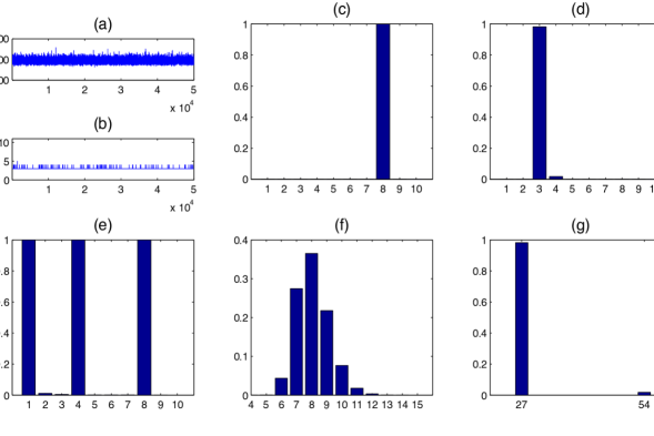
Figure 4: Results of simulation experiments for the case (G) with $C_{0}=3$ categories, true important lags $\{y_{t-1},y_{t-4},y_{t-8}\}$ and sample size $T=500$ for the data set with the median classification error rate. (a) trace plot of marginal likelihood $p({\mathbf{y}}\mid{\mathbf{z}})$; (b) trace plot of the number of important lags; (c) relative frequency distribution of the maximal order; (d) relative frequency distribution of the number of important lags; (e) inclusion proportions of different lags; (f) relative frequency distribution of the number of clusters of the probability kernels $\mbox{\boldmath$\lambda$}_{h_{1},\dots,h_{q}}$; and (g) relative frequency distribution of $\prod_{j=1}^{q}k_{j}$, the number of possible combinations of $(h_{1},\dots,h_{q})$. Panels (c)-(g) are based on thinned samples after burn-in. See Section 2.2 and Section 4 for additional details.

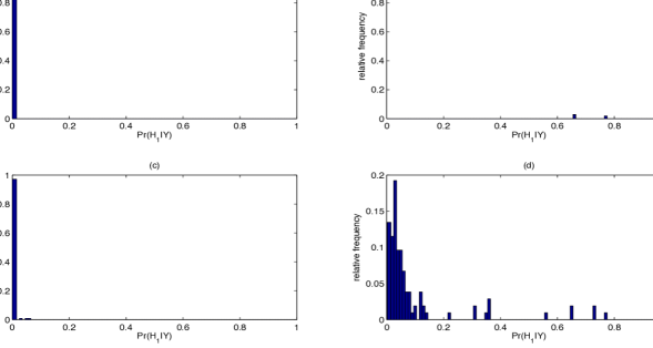
Figure 5: Histograms of posterior probabilities of alternative hypotheses $H_{1}$ based on $100$ simulated data sets for the case (G) with $C_{0}=3$ categories, true important lags $\{y_{t-1},y_{t-4},y_{t-8}\}$ and sample size $T=500$. (a) $H_{0}:$ the lag $y_{t-4}$ is important; (b) $H_{0}:$ the lag $y_{t-5}$ is important; (c) $H_{0}:$ $y_{t-8}$ is an important lag but $y_{t-9}$ and $y_{t-10}$ are not, that is, the chain is of maximal order $8$; and (d) $H_{0}:$ the only important lags are $\{y_{t-1},y_{t-4},y_{t-8}\}$. For the cases (a), (c) and (d), the corresponding $H_{0}$’s were actually true, whereas for the case (b), $H_{0}$ was false. See Sections 3.2 and 4 for additional details.

Figure 4 summarizes the results produced by our method for the case (G) $[3,\{1,4,8\}]$ with $T=500$ data points for the data set corresponding to the median classification error rate. Panels (c)-(e) in Figure 4 illustrate the method’s ability to identify the important lags and the maximal order of the chain.

To assess testing performance, we considered the hypotheses (a) $H_{0}:\widetilde{k}_{4}>1$, (b) $H_{0}:\widetilde{k}_{5}>1$, (c): $H_{0}:\widetilde{k}_{8}>1$ and $\widetilde{k}_{9}=\widetilde{k}_{10}=1$, and (d) $H_{0}:\widetilde{k}_{j}>1$ for $j=1,4,8$ and $\widetilde{k}_{j}=1$ otherwise for the case (G) $[3,\{1,4,8\}]$ described above with $500$ data points. Figure 5 shows histograms of the estimated posterior probabilities of the alternative hypotheses based on $100$ simulated data sets. For the cases (a), (c) and (d), when the corresponding $H_{0}$’s are actually true, the method appropriately assigns values close to zero, whereas for the case (b), when $H_{0}$ is actually false, the estimated posterior probabilities are very close to one.

5 Applications

In this section, we discuss two applications of the proposed conditional tensor factorization approach. In each case, we set the maximal possible order at $q=10$. In experiments with higher values of $q$, the results remained practically unchanged. An additional application of the procedure described in Section 3.2 to test the order of serial dependence in a DNA sequence is presented in Section S.4 of the Supplementary Materials, showing substantially improved results relative to competitors. These data sets have all been analyzed previously in the literature but our proposed nonparametric approach provides new insights into their serial dependence structures. Results produced by the VLMC and the RFMC methods for these data sets are deferred to Section S.5 of the Supplementary Materials.

5.1 Epileptic Seizure Data Set

We first reanalyze a data set from Berchtold and Raftery (2002) (BR), originally presented in McDonald and Zucchini (1997). The data set comprises a binary time series describing whether a patient experienced epileptic seizures on $204$ consecutive days. The two states correspond to either no epileptic seizure or at least one epileptic seizure. BR analyzed the data set using the MTD model and found that $y_{t}$ is best explained by an MTD model with $8$ lags with the lag $y_{t-8}$ being the most important one. The other important lags were $y_{t-1},y_{t-4},y_{t-5}$ and $y_{t-7}$.

Figure 6 summarizes the results obtained by our conditional tensor factorization approach. In agreement with BR, our analysis provides strong evidence for a Markov chain of maximal order $8$ with $y_{t-8}$ being the most important lag with an inclusion probability of one. With an inclusion probability close to $0.85$, $y_{t-1}$ was the second most important predictor. However, in contrast with BR, the distribution of the number of important lags was concentrated around $3$ with the lags $\{y_{t-1},y_{t-4},y_{t-8}\}$ appearing together the maximum number of times. In particular, the inclusion probabilities of $y_{t-5}$ and $y_{t-7}$ were very close to zero suggesting that these lags were not important predictors of $y_{t}$.

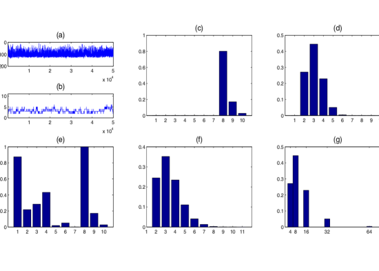
Figure 6: Results for the seizure data set. (a) trace plot of marginal likelihood $p({\mathbf{y}}\mid{\mathbf{z}})$; (b) trace plot of the number of important lags; (c) relative frequency distribution of the maximal order; (d) relative frequency distribution of the number of important lags; (e) inclusion proportions of different lags; (f) relative frequency distribution of the number of clusters of the probability kernels $\mbox{\boldmath$\lambda$}_{h_{1},\dots,h_{q}}$; and (g) relative frequency distribution of $\prod_{j=1}^{q}k_{j}$, the number of possible combinations of $(h_{1},\dots,h_{q})$. Panels (c)-(g) are based on thinned samples after burn-in. See Section 5 for additional details.

5.2 Song of the Wood Pewee Data Set

Next, we reanalyze a data set from Raftery and Tavaré (1994) (RT) that describes the morning song of the wood pewee, a North American song bird, comprising $3$ distinct phrases, labeled $1,2$ and $3$. An interesting feature of the data set is that the series is dominated by two repeating patterns, namely $1312$ and $112$. The repeating patterns indicate strong interactions among the lags and MTD models are not suitable for such data sets. As pointed out by RT, although the first pattern is of length $4$, it can be specified by four transitions of order $2$, namely $1|31,3|12,1|21,2|13$. Likewise, the second repeating pattern $112$ can be defined by the second order transitions $1|12,1|21,2|11$. The transition $1|21$ and the conditioning sequence $12$ appear in both patterns. To accommodate these features, RT modeled the transition probabilities as

$$p(y_{t}=y_{t}\mid y_{t-1}=y_{t-1},y_{t-2}=y_{t-2})=\left\{\begin{array}[]{ll}\alpha_{h}&\text{if}~{}\{y_{t-1},y_{t-2}\}\in A_{h},\\ (1-\alpha_{h})\frac{\pi_{y_{t}}}{\sum_{\{y:(y\mid y_{t-1},y_{t-2})\notin A_{h}\}}\pi_{j}}&\text{if}~{}\{y_{t-1},y_{t-2}\}\in B_{h},\\ \gamma_{y_{t}}&\text{if}~{}\{y_{t-1},y_{t-2}\}=\{1,2\},\\ \pi_{y_{t}}&\text{otherwise},\end{array}\right.$$

where $h=1,2$, $A_{1}=\{1|31,1|21,2|13\}$, $A_{2}=\{2|11\}$, $B_{h}=\{(\widetilde{y}_{t}\mid\widetilde{y}_{t-1},\widetilde{y}_{t-2}):(\widetilde{y}_{t}\mid\widetilde{y}_{t-1},\widetilde{y}_{t-2})\notin A_{h}~{}\text{but there exists}~{}(y_{t}\mid y_{t-1},y_{t-2})~{}\text{with}~{}y_{t-1}=\widetilde{y}_{t-1}~{}\text{and}~{}y_{t-2}=\widetilde{y}_{t-2}\}$, $1\leq\alpha_{h}\leq 1,0\leq\pi_{y}\leq 1,\sum_{y}\pi_{y}=1$ and $0\leq\gamma_{y}\leq 1,\sum_{y}\gamma_{y}=1$. The construction of such complex models with different parameterizations for different conditioning sequences requires critical understanding of the important features of the transition dynamics on a case by case basis and can not be easily generalized.

Figure 7 summarizes the results obtained by applying our conditional tensor factorization approach to the first $500$ data points of the wood pewee data set. Panels (c), (d) and (e) of Figure 7 indicate strong evidence of a Markov chain of maximal order $4$ with three important lags $\{y_{t-1},y_{t-2},y_{t-4}\}$. The inclusion proportions of these three lags were all close to one, whereas the inclusion proportion of the intermediate lag $y_{t-3}$ was close to zero. This suggests that given $\{y_{t-1},y_{t-2},y_{t-4}\}$, $y_{t-3}$ carries little additional information useful for predicting $y_{t}$.

The results can be explained by first noting that a third order representation of the two repeating patterns $1312$ and $112$ comprise the transitions $1|312,3|121,1|213,2|131$ and $1|121,1|211,2|112$, respectively, with the conditioning sequence $121$ appearing in both sets of transitions. A fourth order representation, on the contrary, gives transitions with unique conditioning sequences, namely $1|3121,3|1213,1|2131,2|1312$ and $1|1211,1|2112,2|1121$, respectively. Also, if the third lag $y_{t-3}$ is dropped, we still obtain transitions with unique conditioning sequences, namely $1|31\cdot 1,3|12\cdot 3,1|21\cdot 1,2|13\cdot 2$ and $1|12\cdot 1,1|21\cdot 2,2|11\cdot 1$, respectively. It is thus clear that a Markov chain of maximal order $4$ with three important lags $\{y_{t-1},y_{t-2},y_{t-4}\}$ would provide a good characterization of the transition dynamics of the wood pewee data set, as is captured by the proposed tensor factorization based approach.

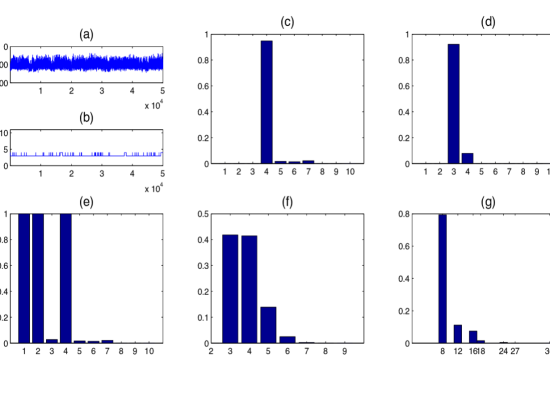
Figure 7: Results for the wood pewee data set. (a) trace plot of marginal likelihood $p({\mathbf{y}}\mid{\mathbf{z}})$; (b) trace plot of the number of important lags; (c) relative frequency distribution of the maximal order; (d) relative frequency distribution of the number of important lags; (e) inclusion proportions of different lags; (f) relative frequency distribution of the number of clusters of the probability kernels $\mbox{\boldmath$\lambda$}_{h_{1},\dots,h_{q}}$; and (g) relative frequency distribution of $\prod_{j=1}^{q}k_{j}$, the number of possible combinations of $(h_{1},\dots,h_{q})$. Panels (c)-(g) are based on thinned samples after burn-in. See Section 5 for additional details.

6 Discussion

The proposed nonparametric Bayesian method provides a flexible yet parsimonious representation of higher order Markov chains, allowing automated identification of the set of important lags while also facilitating testing of many hypotheses of practical interest. In simulation experiments, our method substantially out-performed competitors when there were gaps in the set of important lags, while performing competitively with existing methods in other cases. We have found that such gaps are commonplace in applications we have considered.

While the focus of this paper has been on higher order homogeneous Markov models, the proposed methodology can be easily extended to nonhomogeneous cases in which the transition dynamics is also influenced by exogenous predictors. Indeed, our computer codes already accommodate sequentially varying categorical predictors. Multiple categorical sequences can also be easily accommodated with the sequence label treated as an exogenous sequence specific categorical predictor. Additional important directions of ongoing research include extensions of the methodology to other discrete state space dynamical systems, including higher order hidden Markov models and models for spatial and spatio-temporal categorical data sets.

Supplementary Materials

The Supplementary Materials present some additional figures, describe the approximate two-stage sampler used to determine the starting values of the MCMC sampler, discuss MCMC diagnostics, present an additional application of the proposed methodology, and summarize the results produced by the VLMC and the RFMC methods for the data sets discussed in Section 5.

Appendix

Appendix Appendix A Proof of Theorem 1

Consider a Markov chain $\{y_{t}\}$ of maximal order $q$ with finite state space ${\cal Y}$ and transition probability tensor $P$. Then $\{{\mathbf{s}}_{t}=(y_{t},\dots,y_{t-q+1})^{\rm T}\}$ is a first-order Markov chain with state space ${\cal S}={\cal Y}^{q}$ and transition probability matrix $\widetilde{P}$ with entries

$$\widetilde{P}[(j_{t-1},\dots,j_{t-q}),(i_{t},\dots,i_{t-q+1})]$$

$$=\Pr[(y_{t}=i_{t},\dots,y_{t-q+1}=i_{t-q+1})\mid(y_{t-1}=j_{t-1},\dots,y_{t-q}=j_{t-q})]$$

$$=\left\{\begin{array}[]{ll}P(y_{t}=i_{t}\mid y_{t-1}=j_{t-1},\dots,y_{t-q}=j_{t-q}),&\text{if}~{}i_{t-\ell}=j_{t-\ell}~{}\text{for}~{}\ell=1,\dots,(q-1),\\ 0,&\text{otherwise}.\end{array}\right.$$

The following lemma establishes a general posterior consistency result for first order Markov chain models. With $\widetilde{P}$ and $\widetilde{P}_{0}$ denoting the transition probability matrices of the first order representations of two Markov chains with respective transition probability tensors $P$ and $P_{0}$, we have $d(P,P_{0})=\sum_{{\mathbf{s}}_{1}}\sum_{{\mathbf{s}}_{2}}|\widetilde{P}({\mathbf{s}}_{1},{\mathbf{s}}_{2})-\widetilde{P}_{0}({\mathbf{s}}_{1},{\mathbf{s}}_{2})|$. The conclusion of Theorem 1 thus follows as a consequence.

Lemma 1.

Let $\{y_{t}\}$ be an ergodic Markov chain with finite state space and transition probability matrix $P\in{\cal P}$. Let $\Pi$ be a prior on ${\cal P}$. Then for any $P_{0}$ in the Kullback-Leibler support of $\Pi$ and any $\delta>0$, $\Pi\left\{P:\textstyle d(P,P_{0})>\delta\mid{\mathbf{y}}_{1:T}\right\}\to 0~{}\text{a.s.}~{}P_{0}$.

Proof.

Let ${\cal Y}$ denote the state space of $\{y_{t}\}$. Since $\{y_{t}\}$ is ergodic, it has a unique stationary distribution $\pi_{0}$, with $\pi_{0}(j)>0$ for any $j\in{\cal Y}$. We define the empirical stationary distribution as $\widehat{\pi}_{T}(j)=\sum_{t=1}^{T}1\{y_{t}=j\}/T=n_{j}/T$ for any $j\in{\cal Y}$. Likewise, for any $i,j\in{\cal Y}$, we define the empirical transition probability matrix as $\widehat{P}_{T}(i,j)=\sum_{t=1}^{T}1\{y_{t-1}=i,y_{t}=j\}/\sum_{t=1}^{T}1\{y_{t}=i\}=n_{i,j}/n_{j}$. Define $d_{\pi_{0}}(P,P_{0})=\sum_{i}\sum_{j}\pi_{0}(i)|P(i,j)-P_{0}(i,j)|$ and $K_{\pi_{0}}(P,P_{0})=\sum_{i}\sum_{j}\pi_{0}(i)P_{0}(i,j)\hbox{log}\frac{P(i,j)}{P_{0}(i,j)}=K(\pi_{0}P,\pi_{0}P_{0})$. Also let $V=\{P:d_{\pi_{0}}(P,P_{0})>\delta\min_{i}\pi_{0}(i)\}$. Then $\{P:d(P,P_{0})>\delta\}\subseteq V$. We have

$$\Pi\left\{P:d(P,P_{0})>\delta\mid{\mathbf{y}}_{1:T}\right\}\leq\Pi(V\mid{\mathbf{y}}_{1:T})=\frac{\int_{V}\exp\left\{-T\sum_{i}\sum_{j}\frac{n_{i}}{T}\frac{n_{i,j}}{n_{i}}\hbox{log}\frac{P_{0}(i,j)}{P(i,j)}\right\}d\Pi(P)}{\int_{{\cal P}}\exp\left\{-T\sum_{i}\sum_{j}\frac{n_{i}}{T}\frac{n_{i,j}}{n_{i}}\hbox{log}\frac{P_{0}(i,j)}{P(i,j)}\right\}d\Pi(P)}.$$

(A.2)

By ergodic theorem, $\widehat{\pi}_{T}$ and $\widehat{P}_{T}$ converge almost surely to $\pi_{0}$ and $P_{0}$, respectively (Eichelsbacher and Ganesh, 2002). Therefore, for the numerator, we have

$$\lim_{T\to\infty}\sum_{i}\sum_{j}(n_{i}/T)(n_{i,j}/n_{i})\hbox{log}\{P_{0}(i,j)/P(i,j)\}$$

$$=\lim_{T\to\infty}\sum_{i}\sum_{j}(n_{i}/T)(n_{i,j}/n_{i})\hbox{log}\{(n_{i,j}/n_{i})/P(i,j)\}=\lim_{T\to\infty}K(\widehat{\pi}_{T}\widehat{P}_{T},\widehat{\pi}_{T}P).$$

For any $P\in V$ and $T$ sufficiently large, we have

$$K(\widehat{\pi}_{T}\widehat{P}_{T},\widehat{\pi}_{T}P)\geq d_{\widehat{\pi}_{T}}^{2}(\widehat{P}_{T},P)/4$$

$$\geq\{d_{\widehat{\pi}_{T}}(P,P_{0})-d_{\widehat{\pi}_{T}}(\widehat{P}_{T},P_{0})\}^{2}/4\geq(2\delta/3-\delta/3)^{2}/4=\delta^{2}/36~{}~{}\text{a.s.}~{}P_{0}.$$

Therefore, with $\beta<\delta^{2}/36$, we have

$$\lim_{T\to\infty}\exp(\beta T)\int_{V}\exp\left\{-T\sum_{i}\sum_{j}\frac{n_{i}}{T}\frac{n_{i,j}}{n_{i}}\hbox{log}\frac{P_{0}(i,j)}{P(i,j)}\right\}d\Pi(P)$$

$$\leq\lim_{T\to\infty}\exp\{(\beta-\delta^{2}/36)T\}=0~{}~{}\text{a.s.}~{}P_{0}.$$ (A.3)

Similarly, for the denominator, we have $-\sum_{i}\sum_{j}(n_{i}/T)(n_{i,j}/n_{i})\hbox{log}\{P_{0}(i,j)/P(i,j)\}\to-K_{\pi_{0}}(P_{0},P)>-\epsilon$ a.s. $P_{0}$ for any $P$ with $K_{\pi_{0}}(P_{0},P)<\epsilon$. For any $\beta>0$, choosing $\epsilon=\beta/2$, using Fatou’s lemma we have

$$\exp(\beta T)\int_{{\cal P}}\exp\left\{-T\sum_{i}\sum_{j}\frac{n_{i}}{T}\frac{n_{i,j}}{n_{i}}\hbox{log}\frac{P_{0}(i,j)}{P(i,j)}\right\}d\Pi(P)\to\infty~{}~{}\text{a.s.}~{}P_{0}.$$ (A.4)

The proof follows combining (A.2), (A.3) and (A.4).

Appendix Appendix B Collapsed Conditional of ${\mathbf{k}}$

The two key steps in deriving the collapsed conditional of ${\mathbf{k}}$ in Section 3.1 were (a) to obtain a closed form expression for $p(k_{j}\mid{\mathbf{z}}_{j},{\mathbf{w}}_{j})$ and then (b) to show that $p({\mathbf{k}}\mid{\mathbf{y}},{\mathbf{z}},{\mathbf{z}}^{\star},\mbox{\boldmath$\lambda$}^{\star},\mbox{\boldmath$\pi$}^{\star})=\prod_{j=1}^{q}p(k_{j}\mid{\mathbf{z}}_{j},{\mathbf{w}}_{j})$. Part (b) follows easily by noting that the Markov blanket of $k_{j}$, after $\mbox{\boldmath$\pi$}_{{\mathbf{k}}}$ are integrated out, comprises precisely ${\mathbf{z}}_{j}$ and ${\mathbf{w}}_{j}$. We provide the technical details of the first step here. We use the generic $p_{0}$ to denote priors and hyper-priors. First, we note that integrating out $\mbox{\boldmath$\pi$}_{k_{j}}^{(j)}$ gives

$$p({\mathbf{z}}_{j}\mid{\mathbf{w}}_{j},k_{j})=\int p({\mathbf{z}}_{j}\mid{\mathbf{w}}_{j},\mbox{\boldmath$\pi$}_{k_{j}}^{(j)},k_{j})p_{0}(\mbox{\boldmath$\pi$}_{k_{j}}^{(j)})d\mbox{\boldmath$\pi$}_{k_{j}}^{(j)}=\prod_{r=1}^{C_{0}}\left\{\frac{\Gamma(k_{j}\gamma_{j})}{\{\Gamma(\gamma_{j})\}^{k_{j}}}\frac{\prod_{\ell=1}^{k_{j}}\Gamma\{\gamma_{j}+n_{j,r}(\ell)\}}{\Gamma(k_{j}\gamma_{j}+n_{j,r})}\right\}$$

$$=\prod_{r=1}^{C_{0}}\left\{\frac{1}{(k_{j}\gamma_{j})^{(n_{j,r})}}\prod_{\ell=1}^{\max{\mathbf{z}}_{j,r}}\gamma_{j}^{(n_{j,r}(\ell))}\right\}=\left\{\prod_{r=1}^{C_{0}}\prod_{\ell=1}^{\max{\mathbf{z}}_{j,r}}\gamma_{j}^{(n_{j,r}(\ell))}\right\}\left\{\prod_{r=1}^{C_{0}}\frac{1}{(k_{j}\gamma_{j})^{(n_{j,r})}}\right\},$$ (A.5)

where $x^{(m)}=x(x+1)\dots(x+m-1)$ with $x^{(0)}=1$, ${\mathbf{z}}_{j,r}=\{z_{j,t}:w_{j,t}=r\}$, $n_{j,r}=\sum_{t=t^{\star}}^{T}1\{w_{j,t}=r\}$ denotes the frequency of the $r^{th}$ category of the $j^{th}$ predictor $w_{j}$ and $n_{j,r}(\ell)=\sum_{t=t^{\star}}^{T}1\{z_{j,t}=\ell,w_{j}=r\}$ denotes the number of allocation variables that are associated with the $r^{th}$ category of the $j^{th}$ predictor and are instantiated at $\ell$. Also, since $p(k_{j}\mid{\mathbf{w}}_{j})=p_{0,j}(k_{j})$, we have

$$p({\mathbf{z}}_{j}\mid{\mathbf{w}}_{j})=\sum_{k_{j}=\max_{r}\{{\mathbf{z}}_{j,r}\}}^{C_{0}}p({\mathbf{z}}_{j}\mid{\mathbf{w}}_{j},k_{j})p_{0,j}(k_{j})=\left\{\prod_{r=1}^{C_{0}}\prod_{\ell=1}^{\max{\mathbf{z}}_{j,r}}\gamma_{j}^{(n_{j,r}(\ell))}\right\}U_{n_{j,1},\dots,n_{j,C_{0}}}(\max{\mathbf{z}}_{j}),$$

with $U_{n_{j,1},\dots,n_{j,C_{0}}}(z)=\sum_{k_{j}=z}^{C_{0}}p_{0,j}(k_{j})\prod_{r=1}^{C_{0}}\{\Gamma(k_{j}\gamma_{j})/\Gamma(k_{j}\gamma_{j}+n_{j,r})\}$. This yields a closed form expression for $p(k_{j}\mid{\mathbf{z}}_{j},{\mathbf{w}}_{j})$ as

$$p(k_{j}\mid{\mathbf{z}}_{j},{\mathbf{w}}_{j})=\frac{p(k_{j}\mid{\mathbf{w}}_{j})~{}p({\mathbf{z}}_{j}\mid{\mathbf{w}}_{j},k_{j})}{p({\mathbf{z}}_{j}\mid{\mathbf{w}}_{j})}=\frac{p_{0,j}(k_{j})\prod_{r=1}^{C_{0}}\frac{\Gamma(k_{j}\gamma_{j})}{\Gamma(k_{j}\gamma_{j}+n_{j,r})}}{U_{n_{j,1},\dots,n_{j,C_{0}}}(\max{\mathbf{z}}_{j})},~{}~{}~{}~{}~{}k_{j}=\max{\mathbf{z}}_{j},\dots,C_{0}.$$

(A.6)

This completes the derivation.

Supplementary Materials for
Bayesian Nonparametric Modeling of Higher Order Markov Chains

Appendix S.1 Prior Hyper-parameter $\varphi$

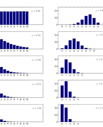
Figure S.1: Induced prior probabilities of different lags to be included in the model ($k_{j}>1$, left panels) and the total number of important lags ($\sum_{j=1}^{q}1\{k_{j}>1\}$, right panels) for the proposed conditional tensor factorization based Markov model with $C_{0}=4$ states and maximal order $q=10$ for various values of $\varphi$ under the prior (16) of the main paper.

Appendix S.2 Approximate Sampler

(a)

(b)

Figure S.2: Graphical model depicting the dependency structure in a second order Markov chain $\{y_{t}\}$ for time point $t$. (a) The proposed model implementing soft clustering of $z_{j,t}\sim\mbox{\boldmath$\pi$}_{k_{j}}^{(j)}(w_{j,t})$ with $\mbox{\boldmath$\pi$}_{k_{j}}^{(j)}(w_{j,t})\sim\hbox{Dir}(\gamma_{j},\dots,\gamma_{j})$ for all $j,w_{j,t}$, and $\mbox{\boldmath$\lambda$}_{h_{1},\dots,h_{q}}\sim\sum_{\ell=1}^{\infty}\pi_{\ell}^{\star}\mbox{\boldmath$\lambda$}_{\ell}^{\star}$ independently for all $(h_{1},\dots,h_{q})$. (b) An approximation of the proposed model implementing hard clustering of $z_{j,t}\sim\widetilde{}\mbox{\boldmath$\pi$}_{k_{j}}^{(j)}(w_{j,t})$ with $\widetilde{\pi}_{h_{j}}^{(j)}(w_{j,t})\in\{0,1\}$ for all $j,h_{j}$ and $w_{j,t}$, and $\mbox{\boldmath$\lambda$}_{h_{1},\dots,h_{q}}\sim\hbox{Dir}(\alpha,\dots,\alpha)$ independently for all $(h_{1},\dots,h_{q})$. This approximation forms the basis of the approximate sampler described in Section S.2 of the Supplementary Materials.

This section describes the approximate sampler used to determine the starting values of the latent class allocation variables ${\mathbf{z}}$ for the MCMC sampler described in Section 3.1 of the main paper.

Given a model indexed by ${\mathbf{k}}=\{k_{1},\dots,k_{q}\}$, the levels of $w_{j}$ are partitioned into $k_{j}$ clusters $\{{\cal C}_{j,r}:r=1,\dots,k_{j}\}$ with each cluster ${\cal C}_{j,r}$ assumed to correspond to its own latent class $h_{j}=r$. With independent Dirichlet priors on the mixture kernels $\mbox{\boldmath$\lambda$}_{h_{1},\dots,h_{q}}\sim\hbox{Dir}(\alpha,\dots,\alpha)$ marginalized out, the likelihood conditional on the cluster configurations ${\cal C}=\{{\cal C}_{j,r}:j=1,\dots,q,r=1,\dots,k_{j}\}$ is given by

$$p({\mathbf{y}}\mid{\cal C})=\prod_{(h_{1},\dots,h_{q})}\frac{\beta\{\alpha+n_{h_{1},\dots,h_{q}}(1),\dots,\alpha+n_{h_{1},\dots,h_{q}}(C_{0})\}}{\beta(\alpha,\dots,\alpha)},$$ (S.1)

where $n_{h_{1},\dots,h_{q}}(y)=\sum_{t=t^{\star}}^{T}1\{y_{t}=y,w_{1,t}\in{\cal C}_{1,h_{1}},\dots,w_{q,t}\in{\cal C}_{m,h_{q}}\}$. Given the current model indexed by ${\mathbf{k}}=\{k_{1},\dots,k_{q}\}$ and clusters ${\cal C}=\{{\cal C}_{j,r}:j=1,\dots,q,r=1,\dots,k_{j}\}$, we do the following for $j=1,\dots,q$.

1. If $k_{j}<C_{0}$, we propose to increase $k_{j}$ to $(k_{j}+1)$. If $k_{j}>1$, we propose to decrease $k_{j}$ to $(k_{j}-1)$. For $1<k_{j}<C_{0}$, the moves are proposed with equal probability. For $k_{j}=1$, the increase move is selected with probability $1$. For $k_{j}=C_{0}$, the decrease move is selected with probability $1$.

2. If an increase move is proposed, we randomly split a cluster of $w_{j}$ into two clusters. We accept this move with acceptance rate based on the approximated marginal likelihood.

3. If a decrease move is proposed, we randomly merge two clusters of $w_{j}$ into a single cluster. We accept this move with acceptance rate based on the approximated marginal likelihood.

The latent class allocation variables ${\mathbf{z}}$ are initialized at the cluster allocation variables returned by the approximate sampler after $100$ iterations.

Appendix S.3 MCMC Diagnostics

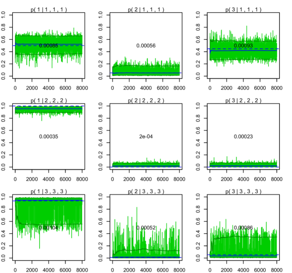
Figure S.3: Trace plots of some transition probabilities for the case (G) with $C_{0}=3$ categories, true important lags $\{y_{t-1},y_{t-4},y_{t-8}\}$ and sample size $T=500$ for the data set with the median classification error rate in the simulation experiments. In each panel, the solid blue line shows the running mean and the horizontal dashed blue line shows the corresponding true value. The darker green lines show the 5% and 95% running quantiles. The number at the middle of each panel shows the Monte Carlo standard error estimated by batch means analysis with batch length 100. See Section 4 of the main paper and Section S.3 of the Supplementary Materials for additional details.

Figure S.3 shows some additional MCMC diagnostics (Cowes and Carlin, 1996; Flegal and Jones, 2011) based on thinned samples for the case (G) with $C_{0}=3$ categories, true important lags $\{y_{t-1},y_{t-4},y_{t-8}\}$ and sample size $T=500$ for the data set with the median classification error rate in the simulation experiments. Our model accommodates uncertainty in the set of important lags. This set may vary from one MCMC iteration to another. To draw the trace plot for $p(y\mid i_{1},i_{4},i_{8})$ accommodating variable lag sets, where $\{i_{1},i_{4},i_{8}\}$ denotes a specific value of $\{y_{t-1},y_{t-4},y_{t-8}\}$, we first identified a $t_{0}$ from $\{(T+1),\dots,N\}$ such that $\{y_{t_{0}-1},y_{t_{0}-4},y_{t_{0}-8}\}=\{i_{1},i_{4},i_{8}\}$. The trace plot for $p(y\mid i_{1},i_{4},i_{8})$ is then based on estimates of $p(y\mid y_{t_{0}-1},y_{t_{0}-2},\dots,y_{t_{0}-10})$ for different MCMC iterations. Our experiments with different $t_{0}$’s with same $\{y_{t_{0}-1},y_{t_{0}-4},y_{t_{0}-8}\}=\{i_{1},i_{4},i_{8}\}$ produced very similar results. As Figure S.3 shows, the running means and quantiles are very stable, Monte Carlo standard errors were small, and there is good agreement between the truth and the running posterior means.

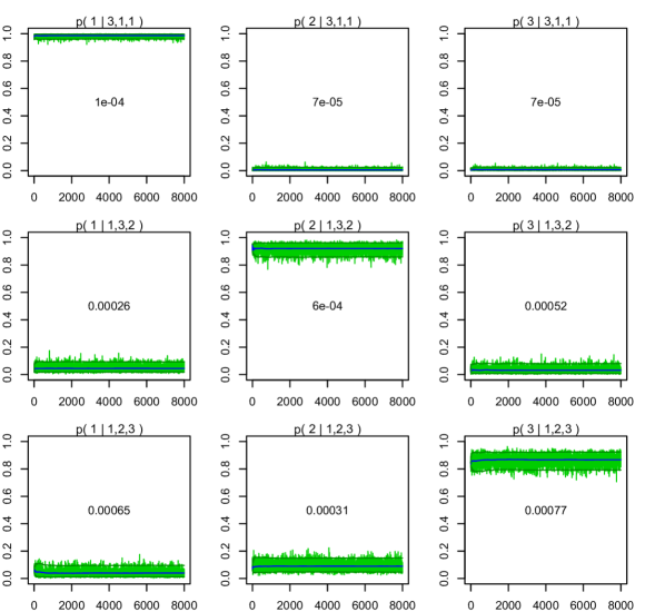
Figure S.4: Trace plots of some transition probabilities for the wood pewee data set. In each panel, the solid blue line shows the running mean. The darker green lines show the 5% and 95% running quantiles. The number at the middle of each panel shows the Monte Carlo standard error estimated by batch means analysis with batch length 100. See Section 4 of the main paper and Section S.3 of the Supplementary Materials for additional details.

Figure S.4 shows similar diagnostic plots for the MCMC output for the wood pewee data set analyzed in Section 5.2 of the main paper. In this case the truth is unknown. Following the discussion in Section 5.2, we assumed $\{y_{t-1},y_{t-2},y_{t-4}\}$ to be the set of important lags. The trace plot for $p(y\mid i_{1},i_{2},i_{4})$ is thus based on the estimates of $p(y\mid y_{t_{0}-1},\dots,y_{t_{0}-10})$ for different MCMC iterations for some $t_{0}$ from $\{T+1,\dots,N\}$ such that $\{y_{t_{0}-1},y_{t_{0}-2},y_{t_{0}-4}\}=\{i_{1},i_{2},i_{4}\}$. The running means and quantiles are again very stable with small Monte Carlo standard errors and the estimated posterior means agree well with our empirical expectations.

In all examples, the quantiles can be used to construct 90% posterior probability regions. Since the transition probabilities have variances uniformly bounded above by $1/4$, Monte Carlo standard errors in the final posterior mean estimates have a conservative uniform upper bound of $1/(2\sqrt{8000})\approx 0.0056$.

Appendix S.4 Analysis of Human Preproglucagon Gene Data Set

In this section, we present an analysis of a DNA sequence found in the human preproglucagon gene (Bell et al.,1983). There are 1752 data points and four states A, C, G and T. Avery and Henderson (1999) and Besag and Mondal (2013) analyzed the data set focusing their attention on Markov models of up to third order, using asymptotic $\chi^{2}$ tests and simulation based exact tests, respectively, to assess fit. The $\chi^{2}$ test of a first order Markov chain against a second order alternative led to rejection of the null hypothesis at the level 0.019, and the test of a second order null versus a third order alternative produced a p-value of 0.34, whereas the corresponding simulation based tests produced p-values of 0.028 and 0.44, respectively, providing evidence that a second order model gives the best fit to the data set among the candidate models.

Figure S.5 summarizes the results produced by the proposed conditional tensor factorization approach with maximal order $q=3$ applied to the first 1000 data points. Due to minor mixing issues, in this case we ran the MCMC algorithm for 5 million iterations (to be conservative) with the initial 2 millions discard as burn-in. The estimated posterior probabilities of first, second and third order Markov models were approximately $0$ (the MCMC chain never visited this model), $0.43$ and $0.57$, respectively. With a posterior odds of $\infty$ for a second order model against a first order model and a posterior odds of $1.33$ for a third order model against a second order model, the results were in general agreement with the frequentist analyses.

The proposed conditional tensor factorization based approach enables us to test for serial dependencies of much higher orders. With the maximal order set at $q=10$, the posterior probability of the model being of maximal order $7$ was estimated to be approximately $0.94$. The MCMC algorithm never visited a Markov model of maximal order $2$. Figure S.6 summarizes the results. Markov models are widely used for nucleotide sequences, and hence the ability to fit more realistic models containing higher order dependence is of substantial importance in this application area.

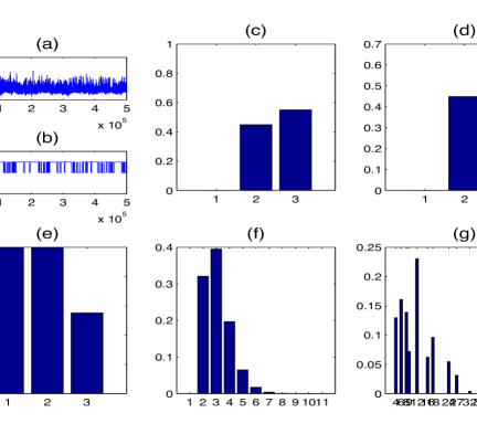
Figure S.5: Results for the human preproglucagon gene data set with the maximal order set at $q=3$. (a) trace plot of marginal likelihood $p({\mathbf{y}}\mid{\mathbf{z}})$; (b) trace plot of the number of important lags; (c) relative frequency distribution of the maximal order; (d) relative frequency distribution of the number of important lags; (e) inclusion proportions of different lags; (f) relative frequency distribution of the number of clusters of the probability kernels $\mbox{\boldmath$\lambda$}_{h_{1},\dots,h_{q}}$; and (g) relative frequency distribution of $\prod_{j=1}^{q}k_{j}$, the number of possible combinations of $(h_{1},\dots,h_{q})$. Panels (c)-(g) are based on thinned samples after burn-in.

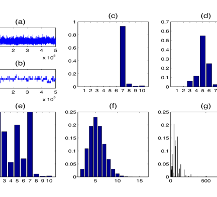
Figure S.6: Results for the human preproglucagon gene data set with the maximal order set at $q=10$. (a) trace plot of marginal likelihood $p({\mathbf{y}}\mid{\mathbf{z}})$; (b) trace plot of the number of important lags; (c) relative frequency distribution of the maximal order; (d) relative frequency distribution of the number of important lags; (e) inclusion proportions of different lags; (f) relative frequency distribution of the number of clusters of the probability kernels $\mbox{\boldmath$\lambda$}_{h_{1},\dots,h_{q}}$; and (g) relative frequency distribution of $\prod_{j=1}^{q}k_{j}$, the number of possible combinations of $(h_{1},\dots,h_{q})$. Panels (c)-(g) are based on thinned samples after burn-in.

Appendix S.5 Results Produced by VLMC and RFMC

Figure S.10 shows the context trees (see Mächler and Bühlmann, 2004) summarizing the serial dependence structures and transition probabilities estimated by the VLMC method, as implemented by the VLMC package in R, applied to the real data sets discussed in Section 5 of the main paper and Section S.4 of the Supplementary Materials. The pruning parameter was selected by AIC criterion.

Figure S.14 shows the relative importance of different lags estimated by the RFMC method, as implemented by the radomForest package in R, applied to the real data sets discussed in Section 5 of the main paper and Section S.4 of the Supplementary Materials.

For the epileptic seizure data set, the wood pewee data set and the human gene data set, the VLMC method estimated Markov chains of maximal orders $9$, $4$ and $4$, respectively. For the seizure data set, the entire sequence consisted of only $204$ data points. With the first $200$ data points used to fit the models, there were not enough additional observations to evaluate prediction performances. For the wood pewee data set and the human gene data set, we used the first $500$ and $1000$ data points to fit the models and the following $500$ observations to evaluate one-step ahead prediction performances. For the wood pewee data set, classification error rates for our proposed conditional tensor factorization based approach, VLMC and RFMC were $0.021$, $0.024$ and $0.026$, respectively. For the human gene data set, classification error rates for our proposed conditional tensor factorization based approach, VLMC and RFMC were $0.64$, $0.66$ and $0.66$, respectively.

While the maximal orders and the classification error rates estimated by the two competing methods are in general agreement, the VLMC method, with a top-down tree based mechanism to model serial dependencies, could not detect gaps in the set of important lags for the first two data sets, which were suggested by the proposed conditional tensor factorization approach. Such gaps seem to be a common feature of many data sets, which is commonly obscured by existing statistical methods.

() Epileptic Seizure Data Set

() Song of the Wood Pewee Data Set

() Human Preproglucagon Gene Data Set

Figure S.10: Context trees produced by the VLMC method for the data sets discussed in Section 5 of the main paper and Section S.4 of the Supplementary Materials.

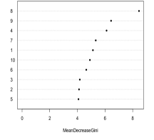
() Epileptic Seizure

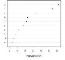
() Song of the Wood Pewee

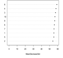
() Human Gene

Figure S.14: Plots showing the relative importance of different lags as estimated by the RFMC method for the data sets discussed in Section 5 of the main paper and Section S.4 of the Supplementary Materials.

Additional References

Bell, I. G., Sanchez-Pescador, R. Laybourn, P. J., and Najarian, R. C. (1983). Exon duplication and divergence in the human preproglucagon gene. Nature, 304, 368-371.

Cowes, M. K. and Carlin, B. P. (1996). Markov chain Monte Carlo convergence diagnostics: A comparative review. Journal of the American Statistical Association, 91, 883-904.

Flegal, M. and Jones, G. (2011). Implementing MCMC: Estimating with confidence. In S. Brooks, A. Gelman, G. Jones, and X. Meng, editors, Handbook of Markov chain Monte Carlo, pages 175-197. Chapman & Hall/CRC Press.

References

- Avery and Henderson (1999) Avery, P. and Henderson, D. (1999). Fitting Markov chain models to discrete state series such as DNA sequences. Applied Statistics, 48, 53–62.
- Berchtold (1995) Berchtold, A. (1995). Autoregressive modeling of Markov chains. In Proc. 10th International Workshop on Statistical Modeling, pages 19–26, New York. Springer.
- Berchtold (1996) Berchtold, A. (1996). Modélisation autorégressive des chaînes de Markov: Utilisation d’une matrice différente pour chaque retard. Revue de Statistique Appliquée, 44, 5–25.
- Berchtold and Raftery (2002) Berchtold, A. and Raftery, A. F. (2002). The mixture transition distribution model for high-order Markov chains and non-Gaussian time series. Statistical Science, 17, 328–356.
- Besag and Mondal (2013) Besag, J. and Mondal, D. (2013). Exact goodness-of-fit tests for Markov chains. Biometrics, 69, 488–496.
- Breiman (2001) Breiman, L. (2001). Random forests. Machine Learning, 45, 5–32.
- Bühlmann and Wyner (1999) Bühlmann, P. L. and Wyner, A. J. (1999). Variable length Markov chains. Annals of Statistics, 27, 480–513.
- De Lathauwer et al. (2000) De Lathauwer, L., De Moore, B., and Vandewalle, J. (2000). A multilinear singular value decomposition. SIAM Journal on Matrix Analysis and Applications, 21, 1253–1278.
- Di Lucca et al. (2013) Di Lucca, M. A., Guglielmi, A., Müller, P., and Quintana, F. A. (2013). A simple class of Bayesian nonparametric autoregression models. Bayesian Analysis, 8, 63–88.
- Eichelsbacher and Ganesh (2002) Eichelsbacher, P. and Ganesh, A. (2002). Bayesian inference for Markov chains. Journal of Applied Probability, 39, 91–99.
- Fahrmier and Kaufmann (1987) Fahrmier, L. and Kaufmann, H. (1987). Regression models for non-stationary categorical time series. Journal of Time Series Analysis, 8, 147–160.
- Ferguson (1973) Ferguson, T. F. (1973). A Bayesian analysis of some nonparametric problems. Annals of Statistics, 1, 209–230.
- George and McCulloch (1997) George, E. and McCulloch, R. (1997). Approaches for Bayesian variable selection. Statistica Sinica, 7, 339–373.
- Ghosh and Ramamoorthi (2003) Ghosh, J. K. and Ramamoorthi, R. V. (2003). Bayesian nonparametrics. Springer Verlag, Berlin.
- Harshman (1970) Harshman, R. (1970). Foundations of the PARAFAC procedure: Models and conditions for an “explanatory” multi-modal factor analysis. UCLA working papers in phonetics, 16, 84.
- Ishwaran and James (2001) Ishwaran, H. and James, L. F. (2001). Gibbs sampling methods for stick-breaking priors. Journal of the American Statistical Association, pages 161–173.
- Jääskinen et al. (2014) Jääskinen, V., Xiong, J., Corander, J., and Koski, T. (2014). Sparse Markov chains for sequence data. Scandinavian Journal of Statistics, 41, 639–655.
- Kass and Raftery (1995) Kass, R. E. and Raftery, A. E. (1995). Bayes factors. Journal of the American Statistical Association, 90, 773–795.
- Liang and Zeger (1986) Liang, K. Y. and Zeger, S. L. (1986). Longitudinal data analysis using generalized linear models. Biometrika, 73, 13–22.
- Liaw and Weiner (2002) Liaw, A. and Weiner, M. (2002). Classification and regression by randomforest. R News, 2, 18–22.
- Mächler and Bühlmann (2004) Mächler, M. and Bühlmann, P. (2004). Variable length Markov chains: methodology, computing, and software. Journal of Computational and Graphical Statistics, 13, 435–455.
- McDonald and Zucchini (1997) McDonald, S. and Zucchini, W. (1997). Hidden Markov and other models for discrete-valued time series. Chapman & Hall, London.
- Miller and Harrison (2015) Miller, J. W. and Harrison, M. T. (2015). Mixture models with a prior on the number of components. ArXiv preprint arXiv:1502.06241.
- Nobile (2004) Nobile, A. (2004). Bayesian finite mixtures with an unknown number of components: The allocation sampler. Annals of Statistics, 32, 2044–2073.
- Nobile and Fearnside (2007) Nobile, A. and Fearnside, A. T. (2007). Bayesian finite mixtures with an unknown number of components: The allocation sampler. Statistics and Computing, 17, 147–162.
- Pitman and Yor (1997) Pitman, J. and Yor, M. (1997). The two-parameter Poisson-Dirichlet distribution derived from a stable subordinator. Annals of Probability, 25, 855–900.
- Quintana and Newton (1998) Quintana, F. A. and Newton, M. A. (1998). Assessing the order of dependence for partially exchangeable binary data. Journal of the American Statistical Association, 93, 194–202.
- Raftery (1985a) Raftery, A. E. (1985a). A model for high-order Markov chains. Journal of the Royal Statistical Society, Series B, 47, 528–539.
- Raftery (1985b) Raftery, A. E. (1985b). A new model for discrete-valued time series autocorrelations and extensions. Rassegna di Metodi Statistici ed Applicazioni, 3-4, 149–162.
- Raftery and Tavaré (1994) Raftery, A. E. and Tavaré, S. (1994). Estimation and modeling repeated patterns in high order Markov chains with the mixture transition distribution model. Applied Statistics, 43, 179–199.
- Richardson and Green (1997) Richardson, S. and Green, P. J. (1997). On Bayesian analysis of mixtures with an unknown number of components. Journal of the Royal Statistical Society, Series B, 59, 731–792.
- Rodriguez and Dunson (2011) Rodriguez, A. and Dunson, D. (2011). Nonparametric Bayesian models through probit stick-breaking processes. Bayesian Analysis, 6, 145–178.
- Ron et al. (1996) Ron, D., Singer, Y., and Tishby, N. (1996). The power of amnesia: Learning probabilistic automata with variable memory length. Machine Learning, 25, 117–149.
- Sethuraman (1994) Sethuraman, J. (1994). A constructive definition of Dirichlet priors. Statistica Sinica, 4, 639–650.
- Stephens (2000) Stephens, M. (2000). Bayesian analysis of mixture models with an unknown number of components - an alternative to reversible jump methods. Annals of Statistics, 28, 40–74.
- Teh (2006) Teh, Y. W. (2006). A hierarchical Bayesian language model based on Pitman-Yor processes. In Proceedings of the Association for Computational Linguistics, pages 985–992.
- Tucker (1966) Tucker, L. (1966). Some mathematical notes on three-mode factor analysis. Psychometrica, 31, 273–282.
- Willems et al. (1995) Willems, F., Shtarkov, Y., and Tjalkens, T. (1995). The context-tree weighting method: Basic properties. IEEE Transactions on Information Theory, 37, 1085–1094.
- Wood et al. (2011) Wood, F., Gasthaus, J., Archambeau, C., Lancelot, J., and Teh, Y. W. (2011). The sequence memoizer. Communications of the ACM, 54, 91–98.
- Xie and Zimmerman (2014) Xie, Y. and Zimmerman, D. L. (2014). Score and Wald tests for antedependence in categorical longitudinal data. Journal of Biometrics and Biostatistics, 5:188, doi:10.4172/2155–6180.1000188.
- Xiong et al. (2015) Xiong, J., Jääskinen, V., and Corander, J. (2015). Recursive learning of sparse Markov chains. Bayesian Analysis. doi:10.4172/2155-6180.1000188.
- Yang and Dunson (2015) Yang, Y. and Dunson, D. B. (2015). Bayesian conditional tensor factorization for high-dimensional classification. Journal of the American Statistical Association. Forthcoming.
- Yee (2010) Yee, T. W. (2010). The VGAM package for categorical data analysis. Journal of Statistical Software, 32, 1–34.
- Zeger and Liang (1986) Zeger, S. L. and Liang, K. Y. (1986). Longitudinal data analysis for discrete and continuous outcomes. Biometrics, 42, 121–130.