Modeling of Resilience Properties in Oscillatory Biological Systems using Parametric Time Petri Nets
Supplementary Information

Abstract

Automated verification of living organism models allows us to gain previously unknown knowledge about underlying biological processes. In this paper, we show the benefits to use parametric time Petri nets in order to analyze precisely the dynamic behavior of biological oscillatory systems. In particular, we focus on the resilience properties of such systems. This notion is crucial to understand the behavior of biological systems (e.g. the mammalian circadian rhythm) that are reactive and adaptive enough to endorse major changes in their environment (e.g. jet-lags, day-night alternating work-time). We formalize these properties through parametric TCTL and demonstrate how changes of the environmental conditions can be tackled to guarantee the resilience of living organisms. In particular, we are able to discuss the influence of various perturbations, e.g. artificial jet-lag or components knock-out, with regard to quantitative delays. This analysis is crucial when it comes to model elicitation for dynamic biological systems. We demonstrate the applicability of this technique using a simplified model of circadian clock.

Appendix 0.A Logical characterization

0.A.1 Notations

The sets ${\rm I\!N}$ and $\mathbb{R}^{+}$ are respectively the sets of natural non-negative real numbers. An interval I of $\mathbb{R}^{+}$ is a $\mathbb{N}$-interval iff its left endpoint belongs to $\mathbb{N}$ and its right endpoint belongs to $\mathbb{N}\cup\{\infty\}$. We set $I^{\downarrow}=\{x|x\in\mathbb{R^{+}},x\leq y$ for some $y\in I\}$, the downward closure of $I$ and $I^{\uparrow}=\{x|x\in\mathbb{R^{+}},x\geq y$ for some $y\in I\}$, the upward closure of $I$. We denote by $\mathcal{I}(\mathbb{N})$ the set of $\mathbb{N}$-intervals of $\mathbb{R}^{+}$.

0.A.2 Parametric time Petri nets with read and logical inhibitor arcs

We consider the model-checking problem of parametric time Petri net with read and logical inhibitor arcs models. This class of models allows us to use parametric temporal bounds for transitions. Therefore, the model-checking procedure addresses the model verification versus the given property together with the parameter synthesis problem. Here we use models that produce only bounded nets, so adding the read and logical inhibition arcs does not add the expressivity to parametric time Petri Nets formalism [2]. A parametric time Petri net with read and logical inhibitor arcs (P-TPN) is a tuple $\mathcal{N}=(\mathbf{P},\mathbf{T},\boldsymbol{\lambda},^{\bullet}\mspace{-2.0mu}(.),(.)^{\bullet},^{\square}\mspace{-2.0mu}(.),\mbox{${}^{\circ}\!(.)$},\allowbreak M_{0},\allowbreak J_{s},\allowbreak D_{\lambda})$, where:

• $\mathbf{P}=\{p_{1},p_{2},\ldots,p_{m}\}$ is a non-empty finite set of places,

• $\mathbf{T}=\{t_{1},t_{2},\ldots,t_{n}\}$ is a non-empty finite set of transitions,

• $\boldsymbol{\lambda}=\{\lambda_{1},\lambda_{2},\ldots,\lambda_{l}\}$ is a finite set of non-negative natural parameters,

• ${}^{\bullet}\mspace{-2.0mu}(.)\in\left(\mathbb{N}^{\mathbf{P}}\right)^{\mathbf{T}}$ is the backward incidence function,

• $(.)^{\bullet}\in\left(\mathbb{N}^{\mathbf{P}}\right)^{\mathbf{T}}$ is the forward incidence function,

• ${}^{\square}\mspace{-2.0mu}(.)\in\left(\mathbb{N}^{\mathbf{P}}\right)^{\mathbf{T}}$ is the read function,

• $\mbox{${}^{\circ}\!(.)$}\in\left(\mathbb{N}^{\mathbf{P}}\right)^{\mathbf{T}}$ is the inhibition function,

• $M_{0}\in\mathbb{N}^{P}$ is the initial marking of the net,

• $J_{s}\in\left(\mathcal{J(\boldsymbol{\lambda})}\right)^{\mathbf{T}}$ is the function that associates a parametric firing interval to each transition,

• $D_{\lambda}\subseteq\mathbb{N}^{\boldsymbol{\lambda}}$ is a convex polyhedron that is the domain of the parameters.

The net $\mathcal{N}$ is parametrized with a set of temporal parameters $\boldsymbol{\lambda}$ together with linear constraints that define the domain $D_{\lambda}$. Linear constraints are given in the form $\gamma=\sum_{i=0}^{l}a_{i}\lambda_{i}\sim b$, where coefficients $a_{i},b\in\mathbb{R}$, $i\in\{1,\ldots,l\}$ and relation $\sim\in\{<,>,\leq,\geq,=\}$. We select the natural subset $D_{\lambda}\subseteq\bar{D}_{\lambda}$ from the set $\bar{D}_{\lambda}\subset{\mathbb{R}}^{\boldsymbol{\lambda}}$ defined by constrains $\gamma$. A valuation of the parameters is a function $\nu:\boldsymbol{\lambda}\mapsto\mathbb{N}_{0}$ that assigns the value to each parameter, i.e. $\left[\nu(\lambda_{1}),\ldots,\nu(\lambda_{l})\right]^{T}\in D_{\lambda}$. We define a parametric time interval as a function $J_{s}:D_{\lambda}\mapsto\mathcal{I}(\mathbb{N})$ that associates an integer interval to each parameter valuation ($\mathcal{I}(\mathbb{N})$ denotes the set of $\mathbb{N}$-intervals).

A marking $M$ of the net is an element of $\mathbb{N}^{P}$ such that $p\in P$ the number of tokens is $M(p)$. A transition $t$ is said to be enabled by the marking $M$ if $\left[\left(M\geq^{\bullet}\mspace{-2.0mu}t\right)\wedge\left(M\geq^{\square}\mspace{-2.0mu}t\right)\wedge\left(M<\mbox{${}^{\circ}\!t$}\right)\right]$, and denoted by $t\in enabled(M)$.

We define the semantics of a P-TPN $\mathcal{N}$ via the semantics of TPN $\llbracket\mathcal{N}\rrbracket_{\nu}$ by assuming the certain valuation of parameters $\nu\in D_{\lambda}$ such that $\llbracket\mathcal{N}\rrbracket_{\nu}=(\mathbf{P},\mathbf{T},\boldsymbol{\lambda},\allowbreak^{\bullet}\mspace{-2.0mu}(.),\allowbreak(.)^{\bullet},\allowbreak^{\square}\mspace{-2.0mu}(.),\allowbreak\mbox{${}^{\circ}\!(.)$},\allowbreak M_{0},\allowbreak I_{s})$, where $\forall t\in\mathbf{T},I_{s}(t)=J_{s}(t)(\nu)$ and

• a transition $t$ is firable if it has been enabled for at least ${}^{\uparrow}{I_{s}}(t)$ time units,

• a transition $t_{k}$ is said to be newly enabled (denoted by $\uparrow enabled(t_{k},M,t_{i})$) by the firing of the transition $t_{i}$ from the marking $M$ if the transition is enabled by the new marking $M^{{}^{\prime}}=M-^{\bullet}\mspace{-2.0mu}t_{i}+t_{i}^{\bullet}$ but was not by $M$. Formally,

  $$\begin{array}[]{l}\uparrow enabled(t_{k},M,t_{i})=\left[\left({}^{\bullet}\mspace{-2.0mu}t_{k}\leq M^{{}^{\prime}}\right)\wedge\left({}^{\square}\mspace{-2.0mu}t_{k}\leq M^{{}^{\prime}}\right)\wedge\left(\mbox{${}^{\circ}\!t_{k}$}>M^{{}^{\prime}}\right)\right]\wedge\\ \left[\left(t_{k}=t_{i}\right)\vee\left({}^{\bullet}\mspace{-2.0mu}t_{k}>M\right)\vee\left({}^{\square}\mspace{-2.0mu}t_{k}>M\right)\vee\left(\mbox{${}^{\circ}\!t_{k}$}\leq M\right)\right].\end{array}$$

  The set of transitions newly enabled by firing the transition $t_{i}$ from the marking $M$ is denoted by $\uparrow enabled(M,t_{i})$,

• a state of TPN is given by the pair $q=(M,I)$ where $M$ is a marking and $I\in(\mathcal{I}(\mathbb{N}))^{\mathbf{T}}$ is an interval function that associates a temporal interval with every transition enabled at $M$.

The semantics of a TPN $\llbracket\mathcal{N}\rrbracket_{\nu}$ can be defined as a time transition system [5] $\mathcal{S}_{\llbracket\mathcal{N}\rrbracket_{\nu}}=(Q,q_{0},\rightarrow)$, where two kinds of transitions are possible: time transitions (when time elapses) and discrete transitions (when a transition of the net is fired), where:

• $Q=\mathbb{N}^{\mathbf{P}}\times\mathcal{I}(\mathbb{N})^{\mathbf{T}}$,

• $q_{0}=\left(M_{0},I_{s}\right)$,

• $\rightarrow\in Q\times(\mathbf{T}\cup\mathbb{N})\times Q$ is the transition relation including a time transition relation and a discrete transition relation. The time transition relation is defined $\forall d\in\mathbb{N}$ as:

  $$\begin{array}[]{l}(M,I)\stackrel{{\scriptstyle d}}{{\longrightarrow}}(M,I^{\prime})\text{ iff }\forall t_{i}\in\mathbf{T},\\ \left\{\begin{array}[]{l}I^{\prime}(t_{i})=\left\{\begin{array}[]{l}({}^{\uparrow}{I^{\prime}(t_{i})},{{I^{\prime}(t_{i})}}^{\downarrow}),\\ \quad{}^{\uparrow}{I^{\prime}(t_{i})}=\max(0,{}^{\uparrow}{I(t_{i})}-d),{{I^{\prime}(t_{i})}}^{\downarrow}={{I(t_{i})}}^{\downarrow}-d,\\ \quad\text{ if }t\in enabled(M),\\ I(t_{i}),\text{ otherwise },\end{array}\right.\\ M\geq^{\bullet}\mspace{-2.0mu}t_{i}\Rightarrow{{I(t_{i})}}^{\downarrow}\geq 0\end{array}\right.\end{array}$$

  The discrete transition relation is defined $\forall t_{i}\in\mathbf{T}$ as:

  $$\begin{array}[]{l}(M,I)\stackrel{{\scriptstyle t_{i}}}{{\longrightarrow}}(M^{\prime},I^{\prime})\text{ iff }\left\{\begin{array}[]{l}t_{i}\in enabled(M),\\ M^{\prime}=M-^{\bullet}\mspace{-2.0mu}t_{i}+t_{i}^{\bullet},\\ {}^{\uparrow}{I(t_{i})}=0,\\ \forall t_{k}\in\mathbf{T},\par I^{\prime}(t_{k})=\left\{\begin{array}[]{l}I_{s}(t_{k})\text{ if }t_{k}\in\uparrow enabled(t_{k},M,t_{i})\\ I(t_{k},)\;\text{, otherwise }\end{array}\right.\end{array}\right.\end{array}$$

0.A.3 Parametric TCTL

In this subsection, we begin by recalling the definition of TPN-TCTL [3], that was inspired by TCTL [1] to tackle bounded time Petri nets. Then we give its parametric version introduced in [8]. These logics have been implemented in the Roméo tool [6], which allows to analyze timed extensions of Petri nets and perform parametric model-checking.

But first, let us define Generalized Mutual Exclusion Constraints, i.e. combinations of conjunctions and/or disjunctions of linear constraints that limit the weighted sum of tokens in a subset of places.

Definition 1 (Gmec )

Let $\mathcal{N}$ be a P-TPN. A Gmec is inductively defined by:

$$\begin{split}\textit{{Gmec}}::=&\left(\sum_{i=1}^{n}a_{i}*M(p_{i})\right)\bowtie c\;|\;\varphi\vee\psi\;|\;\varphi\wedge\psi\;|\;\varphi\Rightarrow\psi\end{split}$$

where $a_{i}\in\mathbb{Z}$, $p_{i}\in\mathbf{P}$, $\bowtie{}\in\left\{{<,\leq,=,>,\geq}\right\}$, $c\in{\rm I\!N}$ and $\varphi,\psi\in\textsc{Gmec}$, the operators ($\vee$,$\wedge$,$\Rightarrow$) having their usual meaning.

Definition 2 (TPN-TCTL )

The temporal logics TPN-TCTL is inductively defined by:

$$\begin{split}\varphi:=\textsc{GMEC}\;|\;\neg\varphi\;|\;\varphi\Rightarrow\psi\;|\;A\varphi\;{U}_{I}\psi\;|\;E\varphi\;{U}_{I}\psi\end{split}$$ (1)

where GMEC is a Gmec, $\varphi,\psi\in\textit{{TPN-TCTL}}$, $I$ is an interval from $\mathbb{N}$ with integer bounds s.t. $[n,m]$, $[n,m[$, $]n,m]$, $]n,m[$, or $[m,\infty[$, $n,m\in{\rm I\!N}$.

The ($\neg$,$\Rightarrow$) operators have their classical meaning and we use the following aliases: $\mathbf{true}=\neg\mathbf{false}$, $EF_{I}\phi=\exists\mathbf{true}\;{\cal U}_{I}\phi$, $AF_{I}\phi=A\mathbf{true}\;{\cal U}_{I}\phi$, $EG_{I}\phi=\neg AF_{I}\neg\phi$, $AG_{I}\phi=\neg EF_{I}\neg\phi$.

This logics can be parametrized the following way:

Definition 3 (PTPN-TCTL )

The parametric temporal logics PTPN-TCTL is inductively defined by:

$$\begin{split}\varphi:=E\varphi\;{U}_{I}\psi\,|\,A\varphi\;{U}_{I}\psi\,|\,EF_{I}\varphi\,|\,AF_{I}\varphi\,|\,EG_{I}\varphi\,|\,AG_{I}\varphi\,|\,\varphi\leadsto_{I_{r}}\psi\end{split}$$ (2)

where $\varphi$ and $\psi$ are Gmec, $I$ and $I_{r}$ are parametric intervals with integer bounds s.t. $[n,m]$, $[n,m[$, $]n,m]$, $]n,m[$, or $[m,\infty[$, $n,m\in{\rm I\!N}$, with the restriction that $I_{r}=[0,m]$ or $I_{r}=[0,\infty[$.

Here, the bounded time response operator $\leadsto_{I_{r}}$ is defined as $AF\left(\varphi\Rightarrow AF_{I_{r}}\psi\right)$.

Appendix 0.B Resilience properties of biological oscillatory systems

0.B.1 Resilience related PTPN-TCTL query specification

Properties A-F introduced in the main body of the paper describe a certain set of behaviors that is normally exposed by the circadian clock model $\mathbb{N}_{CC}$. However we can study the applicability of the model using the parameters in the transition firing interval function. The main external stress in the framework of mammalian circadian clock is light (sunlight or artificial light). The distortion of the normal day-night cycle affects the nominal behavior which causes negative effects like jet-lag. Let us consider how we can model the change of light conditions in the framework of our model.

Query I

Does property $\phi_{\ref{prop:cc_in_absence_of_light}}=\phi_{A}\wedge\phi_{B}\wedge\phi_{C}$ holds when light is always off?

It is known [7] that the circadian clock functions with a period of approximately $24$ hours in the absence of light. In order to check this property we use the different initial state which is also consistent with [4], namely $M(P_{{\texttt{L0}}})=1$, $M(P_{{\texttt{G1}}})=0$ and $M(P_{{\texttt{PC0}}})=1$. We add an observer $O$ that prevents the light from changing its state, $O=\{p_{O}\}$, $M(p_{O})=1$ and $\mbox{${}^{\circ}\!t_{on}$}=p_{O}$. The property is satisfied by the model $\mathbb{N}_{CC}$ with the values of parameters different from those defined under the normal light entrainment.

In order to prevent the certain behavior in the system associated with transitions $T^{\prime}\subset\mathbf{T}$ we add observers $O_{t}=\{P_{O_{t}}\}$, $M(P_{O_{t}})=1$ for each $t\in T^{\prime}$ such that $\mbox{${}^{\circ}\!t$}=P_{O_{t}}$.

Let us now enrich observers with parameters when it is possible. With that, we can check the limits of robustness of a certain system under the perturbed environmental conditions.

Query II

What is the possible duration of the period with light such that $\phi_{\ref{prop:cc_in_absence_of_light}}$ holds?

In order to check this property, we add the observer that substitutes the original transition responsible for switching the light off by another transition $t_{*}$ with the parametric firing interval $J_{s}(t_{*})=[\tau_{d},\tau_{d}]$ such that $O=\{p_{O},t_{*}\}$, $M(p_{O})=1$, $\mbox{${}^{\circ}\!t_{off}$}=p_{O}$, ${}^{\bullet}\mspace{-2.0mu}t_{*}=p_{{\texttt{L1}}}$ and $t^{\bullet}_{*}=p_{{\texttt{L0}}}$. We also have fixed the values of $\tau_{0,1}$ and $\tau_{1,0}$ and $\tau_{g}=1$ to mimic the nominal behavior therefore limiting the possible search space for $\tau_{d}$. This property is satisfied by the model $\mathbb{N}_{CC}$, $\tau_{g}=1$ with $\tau_{d}\in[6,12]$.

The last property we consider addresses the perturbation of the light conditions by switching on the light during ”night” (the period with $M_{P_{{\texttt{L0}}}}=1$ that preserves the nominal behavior).

Query III

For how long can the light be switched on during ”night” such that $\phi_{\ref{prop:cc_in_absence_of_light}}$ holds?

In order to check this property, we add the observer $O_{1}$ that inhibits the transition $t_{on}$ and the observer $O_{2}$ that models switching the light on during ”night”. We show the relevant part of the Petri in Figure 1 (the detailed description of observers is omitted for the sake of readability). This property is satisfied by the model $\mathbb{N}_{CC}$, with $\tau_{g}-\tau_{2}\geq 1$, $\tau_{2}+\tau_{3}\in[0,4]$, where we require $\tau_{1}+\tau_{2}+\tau_{3}=12$. Unfortunately it does not directly answer the stated question and more biologically inspired properties are needed to get more precise parameter estimations.

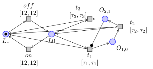
Figure 1: Light switch observer during ”night”.

0.B.2 Model elicitation

We have formulated a series of properties as shown above. By checking them, biologists may gain new inspirations about the underlying biological processes as well as it can be used to make the elicitation of the model that describes certain biological phenomenon. Here we provide the two example for circadian clock model.

Firing delay of transition $t_{g}$.

When introducing the model in Figure 2, we add only one constraint $\gamma=\{\tau_{g}\geq 1\}$ so that it is not instantaneous. We check the property $\phi_{\ref{prop:cc_in_absence_of_light}}$, where we fix the values of oscillation parameters, namely $\tau_{0,1}=18$, $\tau_{1,0}=6$ (property A), $\tau_{0,1}=6$, $\tau_{1,0}=18$ (property B), and $\tau_{0,1}=5$ (property C). However, the parameter synthesis does not give any additional information about the transition $t_{g}$. We construct the observer from property E for the transition $t_{g}$ and check the property $EF_{[0,\infty]}\left(M(p_{O,t_{g}})>0\right)$, and the latter does not hold. Indeed, the only possible value of the parameter $\tau_{g}=0$ is biologically irrelevant. It raises the question about the behaviors where transition $t_{g}$ is needed: it might be relevant only for a certain perturbation of environmental conditions. We modify the model by making the firing intervals of transitions $off$ and $on$ parametric, such that $J_{s}(t_{off})=[\tau_{off},\tau_{off}]$ and $J_{s}(t_{on})=[\tau_{on},\tau_{on}]$, and inducing the additional condition on parameters $\tau_{on}+\tau_{off}=24$. The property is then satisfied for $\tau_{g}\geq 1$, $\tau_{on}\in[7,11]$ and $\tau_{g}\geq 1$, $\tau_{on}=23$. This shows that the model provided in [4] initially allows for various biologically relevant behaviors.

Firing delay of transition $t_{a}$.

The model checking of property E shows that it is only satisfied with the zero firing delay $\tau_{a}=0$ of the transition $t_{a}$. As in the previous example, we may ask the question about the environmental light conditions that allow for the firing of transition $t_{a}$ with the initial firing delay $\tau_{a}=7$. We check the property $EF_{[0,\infty]}\left(M(p_{O,t_{a}})>0\right)$, where the observer for transition $t_{a}$ is constructed in the same fashion as in property E. It is then satisfied with $\tau_{on}\in\{23,24\}$. The case $\tau_{on}=24$ corresponds to property I where circadian clock in constant darkness is considered. We see that the set of admissible behaviors such that $t_{a}$ is eventually fired is larger than we predicted. It shows as well that the model in [4] has a certain redundancy that allows to address the change of environmental conditions. Having enough biologically relevant knowledge it may be possible to define the delays of all transitions in the system using this approach.

This work-flow can be applied to any P-TPN model that describes gene regulatory network. Having enough biological knowledge that can be formalized in terms of PTPN-TCTL properties, such models can be refined together with the limits of their applicability. Model checking procedures can not address the pure inference problem, therefore this preliminary knowledge is needed.

0.B.3 Effects of gene knock-out and artificial jet-lag

The observers introduced above allow to study the behavior of the system after the gene knock-out and under the effect of artificial jet-lag. The effect of gene knock-out can be modeled by simply suppressing all the behaviors that allow the set of genes G to change its state from $0$ to $1$, that is by suppressing transitions $t_{b}$ and $t_{f}$. The behavior of the system $\mathbb{N}_{CC}$ is then restricted only to changes of light state and there is no permanent oscillations of protein PC which means that gene knock-out leads to the system malfunction.

Let us discover the effect of artificial jet-lag on the model, when the duration of the period with light is prolonged (since the period without light does not affect the standard behavior much). We assume that there are no perturbations during first $24$ time units, then the light is switched on for $30$ time units and after that the system returns to the nominal behavior. This effect can be modeled in a similar way to query I. We add the observer that prevents the light from switching off after $24$ time units and allows it again after $16$ time units. In this way it is guaranteed that $M(p_{{\texttt{L1}}})=1$ for $30$ time units without any switching. We show the relevant part of the Petri net with the observer in Figure 2. Checking the property A shows that the system does not function normally as the time for PC to change the state from $0$ to $1$ is $\tau_{0,1}\geq 36$. This corresponds to the fact that $t_{c}$ is the only transition that changes the state of PC from $0$ to $1$ and it is enabled only when light is switched off. It is important to notice that P-TPN formalism does not allow to model the recovery process of the system since it is ruled by local clocks only. For instance, if the delay observer ${}^{\prime}O$ is added with a delay of $100$ time units, the result of model checking the property A after this delay refers to the standard behavior, i.e. $\tau_{0,1}\geq 18$.

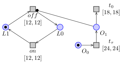
Figure 2: Artificial jet-lag observer

0.B.4 Resilience in PTPN-TCTL formalism

Here we stated the number of properties that describe the standard behavior of the circadian clock model such as permanent oscillation and entrainment properties of the set of genes G. Please note that we can judge only about certain local time properties meaning that there is no notion of the global clock in P-TPN models. Due to the limited expressivity of PTPN-TCTL, we enrich the model with observers that are given in a fairly general fashion. We also addressed the limits of the model applicability by enriching the observers with parameters that are determined by parameter synthesis procedure. It allows us to verify resilience related properties such as robustness to changes in the environmental conditions.

References

- [1] Alur, R., Courcoubetis, C., Dill, D.: Model-checking for real-time systems. In: Logic in Computer Science, 1990. LICS’90, Proceedings., Fifth Annual IEEE Symposium on Logic in Computer Science. pp. 414–425. IEEE (1990)
- [2] Bérard, B., Cassez, F., Haddad, S., Lime, D., Roux, O.H.: The expressive power of time petri nets. Theoretical Computer Science 474, 1–20 (2013)
- [3] Boucheneb, H., Gardey, G., Roux, O.H.: TCTL model checking of time petri nets. Journal of Logic and Computation 19(6), 1509–1540 (2009)
- [4] Comet, J.P., Bernot, G., Das, A., Diener, F., Massot, C., Cessieux, A.: Simplified models for the mammalian circadian clock. Procedia Computer Science 11, 127–138 (2012)
- [5] Larsen, K.G., Pettersson, P., Yi, W.: Model-checking for real-time systems. In: Fundamentals of computation theory, pp. 62–88. Springer (1995)
- [6] Lime, D., Roux, O.H., Seidner, C., Traonouez, L.M.: Romeo: A parametric model-checker for Petri nets with stopwatches. In: Tools and Algorithms for the Construction and Analysis of Systems, pp. 54–57. Springer (2009)
- [7] Oster, H., Yasui, A., van der Horst, G.T.J., Albrecht, U.: Disruption of mCry2 restores circadian rhythmicity in mPer2 mutant mice. Genes & Development 16(20), 2633–2638 (2002)
- [8] Traonouez, L.M., Lime, D., Roux, O.H.: Parametric model-checking of stopwatch Petri nets. Journal of Universal Computer Science 15(17), 3273–3304 (2009)