Abstract

We study nonparametric estimation of the distribution function (DF) of a continuous random variable based on a ranked set sampling design using the exponentially tilted (ET) empirical likelihood method. We propose ET estimators of the DF and use them to construct new resampling algorithms for unbalanced ranked set samples. We explore the properties of the proposed algorithms. For a hypothesis testing problem about the underlying population mean, we show that the bootstrap tests based on the ET estimators of the DF are asymptotically normal and exhibit a small bias of order $O(n^{-1})$. We illustrate the methods and evaluate the finite sample performance of the algorithms under both perfect and imperfect ranking schemes using a real data set and several Monte Carlo simulation studies. We compare the performance of the test statistics based on the ET estimators with those based on the empirical likelihood estimators.

Keywords: Distribution function; Exponential tilting; Imperfect ranking; Ranked set sample.

1 Introduction

Ranked set sampling (RSS) is a powerful and cost-effective data collection technique that is often used to collect more representative samples from the underlying population when a small number of sampling units can be fairly accurately ordered without taking actual measurements on the variable of interest. RSS is most effective when obtaining exact measurement on the variable of interest is very costly, but ranking the sampling units is relatively inexpensive. RSS finds applications in industrial statistics, environmental and ecological studies as well as medical sciences. For recent overviews of the theory and applications of RSS and its variations see Wolfe (2012) and Chen et al. (2004).

Ranked set samples can be either balanced or unbalanced. An unbalanced ranked set sample (URSS) is one in which the ranked order statistics are not quantified the same number of times. To obtain an URSS of size $n$ from the underlying population we proceed as follows. Let $n$ sets of sampling units, each of size $k$, be randomly chosen from the population using a simple random sampling (SRS) technique. The units of each set are ranked by any means other than the actual quantification of the variable of interest. Finally, one and only one unit in each ordered set with a pre-specified rank is measured. Let $m_{r}$ be the number of measurements on units with rank $r$, $r\in\{1,\ldots,k\}$ such that $n=\sum_{r=1}^{k}m_{r}$. Suppose $X_{(r)j}$ denotes the measurement on the $j$th unit with rank $r$. The resulting URSS of size $n$ from the underlying population is denoted by ${\bf X}_{URSS}=\{\mathcal{X}_{1},\ldots,\mathcal{X}_{n}\}$, where the elements of the $r$th row $\mathcal{X}_{r}=(X_{(r)1},X_{(r)2},\ldots,X_{(r)m_{r}})$ are independently and identically distributed (i.i.d.) from $F_{(r)},r=1,\ldots,k$ and $F_{(r)}$ is the DF of the $r$th order statistic. Moreover, $X_{(r)j}$s are independent for $r=1,\ldots,k$ and $j=1,\ldots,m_{r}$. Note that if $m_{r}=m$, $r=1,\ldots,k$, then URSS reduces to the balanced RSS. The DF of URSS is

$$\widehat{F}_{q_{n}}(t)=\frac{1}{n}\sum_{r=1}^{k}\sum_{j=1}^{m_{r}}I(X_{(r)j}\leq t)=\sum_{r=1}^{k}q_{m_{r}}\widehat{F}_{(r)}(t),$$ (1)

where $n=\sum m_{r}$ and $q_{m_{r}}=m_{r}/n$. As it is shown in Chen et al. (2004), when $n\longrightarrow\infty$, and $q_{m_{r}}\longrightarrow q_{r}$, for $r=1,\ldots,k$, we have $\widehat{F}_{q_{n}}(t)\longrightarrow F_{q}(t)$, where

$$F_{q}(t)=\sum_{r=1}^{k}q_{r}F_{(r)}(t).$$ (2)

One can easily see that $F_{q}(t)$ is not equal to the underlying DF $F(t)$, unless $q_{r}=1/k$, $r=1,\ldots,k$, showing that the EDF based on the URSS data does not provide a good estimate of the underlying distribution $F$. The properties of the EDF of the balanced and unbalanced RSS are studied in Stokes and Sager (1988) as well as Chen et al. (2004).

In this paper, we use the empirical likelihood method as a nonparametric approach for estimating $F$. To this end, we propose two methods to estimate $F$ using the exponentially tilted (ET) technique. The proposed estimators can be used as standard tools for practitioners to estimate the standard error of any well-defined statistic based on RSS or URSS data and to make inferences about the characteristics of interest of the underlying population. Another interesting problem in this direction is to develop efficient resampling techniques for URSS data, as in many cases the exact or the asymptotic distribution of the statistics based on URSS data are not available or they are very difficult to obtain (e.g., Chen et al., 2004). Akin to the methods of Modarres et al. (2006) and Amiri et al. (2014), the new ET estimators of $F$ are used to construct new resampling techniques for URSS data. We study different properties of the proposed algorithms. For a hypothesis testing problem, about the underlying population mean, we show that the bootstrap tests based on the ET estimators are asymptotically normal and exhibit a small bias of order $O(n^{-1})$ which are desirable properties.

The outline of the paper is as follows. In Section 2, we present ET estimators of $F$ based on the URSS data. Section 3 considers two methods for resampling RSS and URSS data based on the ET estimators of $F$. We provide justifications for validity of these methods for a hypothesis testing problem about the population mean. Section 4 describes a simulation study to compare the finite sampling properties of the proposed methods with parametric bootstrap and some existing resampling techniques for testing a hypothesis about the population mean. We consider both perfect and imperfect ranking scenarios, three different distributions and five RSS designs. We compare the performance of our proposed methods with the one based on the empirical likelihood method studied in Liu et al. (2009) as well as Baklizi (2009). In Section 5, we apply our methods for a testing hypothesis problem using a real data set consisting of the birth weight and seven-month weight of 224 lambs along with the mother’s weight at time of mating. Section 6 provides some concluding remarks.

2 Exponential Tilting of DF

Exponential tilting of an empirical likelihood is a powerful technique in nonparametric statistical inference. The impetus of this approach is the use of the estimated DF subject to some constraints rather than the EDF. ET methods find applications in computation of bootstrap tail probabilities (Efron and Tibshirani, 1993), point estimation (Schennach, 2007), estimation of the spatial quantile regression (Kostov, 2012), Bayesian treatment of quantile regression (Schennach, 2005), small area estimation (Chaudhuri and Ghosh, 2011) and Calibration estimation (Kim, 2010), among others.

Let ${\bf X}=\{X_{1},\ldots,X_{n}\}$ be a generic sample of size $n$ from $F$ and suppose $F_{n}(x)=\sum_{i=1}^{n}\frac{1}{n}\mathbb{I}(X_{i}\leq x)$ is the EDF of ${\bf X}$ which places empirical frequencies (weights) $1/n$ on each $X_{i}$. Consider an estimator $\widetilde{F}_{p}(x)=\sum_{i=1}^{n}p_{i}\mathbb{I}(X_{i}\leq x)$ of $F$ which assigns weights $p_{i}$ instead of $1/n$ to each $X_{i}$. To obtain the ET estimator of $F$, we minimize an aggregated distance between the empirical weights $1/n$ and $p_{i}$ subject to some constraints on the $p_{i}$’s. More specifically, one chooses a distance $d(\widetilde{F}_{p},F_{n})=\sum_{i=1}^{n}d(p_{i},\frac{1}{n})$ and minimizes $d(\widetilde{F}_{p},F_{n})$ subject to $\sum_{i=1}^{n}p_{i}=1$ and some other constrains such as $g({\bf X},\theta_{0})=\sum_{i=1}^{n}p_{i}g(X_{i},\theta_{0})=0$, using the following Lagrangian multiplier method

$$d(\widetilde{F}_{p},F_{n})-\lambda g({\bf X},\theta_{0})-\alpha\big{(}\sum_{i=1}^{n}p_{i}-1\big{)},$$ (3)

where $g({\bf X},\theta_{0})$ is often imposed under the null hypothesis in a testing problem or any other conditions that one needs to account for in practice. Note that the minimization in (3) can also be done by minimizing the distance between $\widetilde{F}_{p}(x)$ and any target estimator $F_{\widehat{p}}(x)=\sum_{i=1}^{n}\widehat{p}_{i}\mathbb{I}(X_{i}\leq x)$ other than the EDF $F_{n}(t)$.

The choice of the discrepancy function $d(\cdot,\cdot)$ for the aggregated loss $d(\widetilde{F}_{p},F_{n})$ in (3) leads to different ET estimators of $F$. Since $F_{n}(x)$ is the nonparametric maximum likelihood estimator of $F$ under the Kullback-Leibler distance subject to the restriction $\sum_{i=1}^{n}p_{i}=1$, one often uses

$$d(\widetilde{F}_{p},F_{\widehat{p}})=\sum_{i=1}^{n}p_{i}\log\left(\frac{p_{i}}{\widehat{p}_{i}}\right).$$

We propose two ET estimators of $F$ based on URSS data with sample size $n=\sum_{r=1}^{k}m_{r}$ where $k$ is the set size. The ET estimators are then used to propose new bootstrapping algorithms from URSS data.

2.1 Exponential Tilting of All Observations (EAT)

In this section, we propose our first ET estimator of $F$ which is later used to resample from within each row of ${\bf X}_{URSS}=\{X_{(r)j},r=1,\ldots,k;j=1,\ldots,m_{r}\}$. The idea behind the first ET estimator of $F$, for bootstrapping ${\bf X}_{URSS}$, is to find an estimator

$$\widetilde{F}_{p}(x)=\sum_{r=1}^{k}\sum_{j=1}^{m_{r}}p_{(r)j}\mathbb{I}(X_{(r)j}\leq x),$$ (4)

subject to the constraints

$$\sum_{r=1}^{k}\sum_{j=1}^{m_{r}}p_{(r)j}=1\quad\text{and}\quad\sum_{r=1}^{k}\sum_{j=1}^{m_{r}}p_{(r)j}X_{(r)j}=\overline{{X}}_{URSS},$$ (5)

where $\overline{X}_{URSS}=\displaystyle\frac{1}{n}\sum_{r=1}^{k}\sum_{j=1}^{m_{r}}X_{(r)j}$.

Lemma 1.

Let ${\bf X}_{URSS}=\{X_{(r)j},r=1,\ldots,k;j=1,\ldots,m_{r}\}$ be a URSS sample of size $n$ from the underlying population $F$ when the set size is $k$ and $X_{(r)j}\in{\bf R}$ is the $r$-th order statistic in a simple random sample of size $k$ from $F$. The optimum values of $p_{(r)j}$ in (4) under the constraints (5) are given by

$$\tilde{p}_{(r)j}=\frac{\exp(\lambda X_{(r)j})}{\displaystyle\sum_{r=1}^{k}\sum_{j=1}^{m_{r}}\exp(\lambda X_{(r)j})},\quad r=1,\ldots,k;~{}j=1,\ldots,m_{r},$$ (6)

where $\lambda$ is obtained from $\sum_{r=1}^{k}\sum_{j=1}^{m_{r}}p_{(r)j}X_{(r)j}=\overline{X}_{URSS}$.

Proof.

Using the Lagrange multipliers method, and by minimizing

$$\sum_{r=1}^{k}\sum_{j=1}^{m_{r}}p_{(r)j}\ln\left(\frac{p_{(r)j}}{1/n}\right)+\lambda(\sum_{r=1}^{k}\sum_{j=1}^{m_{r}}p_{(r)j}X_{(r)j}-\overline{X}_{URSS})+\alpha(\sum_{r=1}^{k}\sum_{j=1}^{m_{r}}p_{(r)j}-1),$$ (7)

with respect to $p_{(r)j}$’s, one can easily obtain the optimum values in (6). ∎

In Section 3, we use $\tilde{F}_{p}(x)=\sum_{r=1}^{k}\sum_{j=1}^{m_{r}}\tilde{p}_{(r)j}\mathbb{I}(X_{(r)j}\leq x)$ for bootstrapping $X_{URSS}$ instead of the commonly used empirical DF. It is worth noting that for hypothesis testing problems about the underlying population mean $\mu$ involving the null hypothesis $H_{0}:\mu=\mu_{0}$, minimization in (7) is done subject to the condition $\sum_{r=1}^{k}\sum_{j=1}^{m_{k}}p_{(r)j}X_{(r)j}=\mu_{0}$. Using the optimum weights $\widetilde{p}_{(r)j}$ from the ET estimate of $F$, we also propose $S^{2}=\sum_{r=1}^{k}\sum_{j=1}^{m_{r}}\tilde{p}_{(r)j}(X_{(r)j}-\overline{X}_{URSS})^{2}$ to estimate the population variance $\sigma^{2}$.

2.2 Exponential Tilting of Rows (EAR)

By the structure of the URSS data, ${\bf X}_{URSS}$, we observe that $X_{(r)1},\ldots,X_{(r)m_{r}}$ are i.i.d.  samples from $F_{(r)}(\cdot)$, which is the distribution of the $r$-th order statistic in a simple random sample of size $k$ from $F$. Since

$$F(t)=\frac{1}{k}\sum_{r=1}^{k}F_{(r)}(t),$$

the idea behind our next proposed ET estimator of $F$ is to estimate each $F_{(r)}$ using $X_{(r)1},\ldots,X_{(r)m_{r}}$, and construct an estimator of $F$ by averaging over these estimators using suitable weights obtained from the Lagrange multipliers method under some constraints. To this end, we work with an estimator of $F$ of the form

$$\widetilde{F}_{p}(t)=\sum_{r=1}^{k}p_{(r)}\widehat{F}_{(r)}(t),$$ (8)

where $\widehat{F}_{(r)}(t)=\frac{1}{m_{r}}\sum_{j=1}^{m_{r}}\mathbb{I}(X_{(r)j}\leq t)$ is the EDF of $X_{(r)1},\ldots,X_{(r)m_{r}}$.

Lemma 2.

Let ${\bf X}_{URSS}=\{X_{(r)j},r=1,\ldots,k;j=1,\ldots,m_{r}\}$ be a URSS sample of size $n$ from $F$ where the set size is $k$ and $\{X_{(r)j},j=1,\ldots,m_{r}\}$ are i.i.d. samples from $F_{(r)}$ the DF of the $r$-th order statistic of a simple random sample of size $k$ from $F$. Then, an optimum estimator of $F$ in the form of (8) under the constraints $\sum_{r=1}^{k}p_{(r)}=1$ and $\sum_{r=1}^{k}p_{(r)}\bar{X}_{(r)}=\overline{X}_{URSS}$, where $\overline{X}_{(r)}=\frac{1}{m_{r}}\sum_{j=1}^{m_{r}}X_{(r)j}$, $r=1,\ldots,k$, is given by

$$\tilde{F}_{p}(x)=\displaystyle\sum_{r=1}^{k}\frac{\tilde{p}_{(r)}}{m_{r}}\sum_{j=1}^{m_{r}}\mathbb{I}(X_{(r)j}\leq x)\quad\text{with}\quad\tilde{p}_{(r)}=\frac{\exp(\lambda\overline{X}_{(r)})}{\sum_{r=1}^{k}\exp(\lambda\overline{X}_{(r)})},$$ (9)

where $\lambda$ is obtained from $\sum_{r=1}^{k}p_{(r)}\overline{X}_{(r)}=\overline{X}_{URSS}$.

Proof.

The results easily follow using the Lagrange multipliers method and minimizing

$$\sum_{r=1}^{k}p_{(r)}\ln\left(\frac{p_{(r)}}{1/k}\right)+\lambda(\sum_{r=1}^{k}p_{(r)}\overline{X}_{(r)}-\overline{X}_{URSS})+\alpha(\sum_{r=1}^{k}p_{(r)}-1).$$ (10)

with respect to $p_{(r)}$. ∎

In Section 3, we use $\tilde{F}_{p}(x)=\displaystyle\sum_{r=1}^{k}\frac{\tilde{p}_{(r)}}{m_{r}}\sum_{j=1}^{m_{r}}\mathbb{I}(X_{(r)j}\leq x)$ and propose a new bootstrapping algorithm to resample from $X_{URSS}$ instead of the commonly used empirical DF. Here again for hypothesis testing problems involving $H_{0}:\mu=\mu_{0}$ where $\mu$ is the population mean, minimization in (10) is done subject to the condition $\displaystyle\sum_{r=1}^{k}p_{(r)}\overline{X}_{(r)}=\mu_{0}$.

Remark 1.

If for the observed URSS data all the $m_{r}$s are large enough, then one can use ET estimators of $F_{(r)}$ by simply treating $X_{(r)j}$’s as a SRS of size $m_{r}$ from $F_{(r)}$ and constructing the estimator $\widetilde{F}(t)=\frac{1}{k}\sum_{r=1}^{k}\widetilde{F}_{(r)}(t)$ for $F$. Here, $\widetilde{F}_{(r)}(t)=\sum_{j=1}^{m_{r}}w_{j}(r)\mathbb{I}(X_{(r)j}\leq t)$ and $w_{j}(r)$s are obtained subject to constraints $\sum_{j=1}^{m_{r}}w_{j}(r)=1$ and $\sum_{j=1}^{m_{r}}w_{j}(r)X_{(r)j}=\overline{X}_{(r)}$, for $r=1,\ldots,k$, using the following Lagrange multipliers problems:

$$\sum_{j=1}^{m_{r}}w_{j}(r)\ln\left(\frac{w_{j}(r)}{1/m_{r}}\right)+\lambda_{r}(\sum_{j=1}^{m_{r}}w_{j}(r)\overline{X}_{(r)j}-\overline{X}_{(r)})+\alpha_{r}(\sum_{j=1}^{m_{r}}w_{j}(r)-1),\quad r=1,\ldots,k.$$

3 Bootstrapping URSS and RSS

In this section, we propose two new bootstrapping techniques to resample from a balanced or unbalanced ranked set sample of size $n$. The first algorithm is based on the ET estimator of $F$ in Lemma 1 to resample the entire URSS while the second one uses the ET estimator of $F$ in Lemma 2 to resample from within each row separately. We note that most of the bootstrap methods developed for RSS are based on the EDF and one can easily modify them using ET estimators of $F$. Monte Carlo simulation studies indicate that bootstrapping methods based on the ET estimators of $F$ perform better than their counterparts using the EDF.

3.1 Bootstrapping Algorithm: EAT

To resample from the ET estimator of $F$ given by

$$\tilde{F}_{p}(x)=\displaystyle\sum_{r=1}^{k}\sum_{j=1}^{m_{r}}\tilde{p}_{(r)j}\mathbb{I}(X_{(r)j}\leq x),$$

where $\tilde{p}_{(r)j}$ is defined in (6) we proceed as follows:

• Assign probability $\tilde{p}_{(r)j}$ to each element $X_{(r)j}$ of ${\bf X}_{URSS}$.

• Randomly draw $X_{1}^{\diamond},\ldots,X_{k}^{\diamond}$ from ${\bf X}_{URSS}$ according to probabilities $\{\tilde{p}_{(r)j}\}$, order them as $X_{(1)}^{\diamond}\leq\ldots\leq X_{(k)}^{\diamond}$ and retain $X^{*}_{(r)1}=X_{(r)}^{\diamond}$.

• Repeat Step 2, for $r=1,\ldots,k$ and $j=1,\ldots,m_{r}$ to generate a bootstrap URSS $\left\{X^{*}_{(r)j}\right\}$.

• Repeat steps 2-3, $B$ times to obtain the bootstrap samples.

One can easily validate the use of the ET estimator of $F$ for different bootstrapping purposes. For example, suppose we want to carry out a bootstrap test for testing $H_{0}:\mu=\mu_{0}$ against $H_{a}:\mu>\mu_{0}$, where $\mu$ is the unknown parameter of interest. Using Hall (1992), the Edgeworth expansion of the $p$-value for testing $H_{0}$ against $H_{a}$ based on a SRS of size $mk$ from the underlying population with the test statistic $T=\frac{\bar{X}-\mu_{0}}{S/\sqrt{mk}}$, is given by

$$P=P(T\geq t)=1-\Phi(t)-(mk)^{-1/2}q(t)\phi(t)+O(\frac{1}{mk}),$$ (11)

where $q(\cdot)$ is a quadratic function and $\Phi(\cdot)$ and $\phi(\cdot)$ are the standard normal distribution and density functions, respectively. We consider the problem for a balanced RSS case, as the following argument can also be applied to URSS data with some modifications. Let $\{X_{(r)j},r=1,\ldots,k;~{}j=1,\ldots,m\}$ be a balanced ranked set sample of size $mk$ from the underlying population with mean $\mu$. We show that the ET bootstrap approximation of the sampling distribution of $T$ is in error by only $1/mk$ and the $p$-value obtained through the EAT method has the desirable second order accuracy This is similar to results obtained in DiCiccio and Romano (1990). For more details see Efron (1981) and Feuerveger et al. (1999).

Proposition 1.

Suppose $\{X^{*}_{(r)j},r=1,\ldots,k;~{}j=1,\ldots,m\}$ is a bootstrap sample generated from the EAT algorithm. Let $T^{*}=\frac{(\bar{X}^{*}-\bar{X})}{S^{*}/\sqrt{mk}}$ be the bootstrap test for testing $H_{0}:\mu=\mu_{0}$ with p-value $P^{*}$, where $\bar{X}^{*}$ is the mean of the bootstrap sample obtained form the ET estimator of $F$ and $S^{2*}=\frac{1}{k}\sum_{r=1}^{k}S^{2*}_{(r)}$ with $S^{2*}_{(r)}=\frac{1}{m-1}\sum_{j=1}^{m}(X^{*}_{(r)j}-\bar{X}^{*}_{(r)})^{2}$. Then,

$$P-P^{*}=O(\frac{1}{mk}),$$ (12)

where $P$, given by (11), is the p-value of the usual $T$-test based on a simple random sample of comparable size $mk$ from the underlying population.

Proof.

For simplicity, we write the resampled data as $\{X_{1}^{*},\ldots,X_{km}^{*}\}$. In order to test $H_{0}:\mu=\mu_{0}$, and to ensure that the null hypothesis is incorporated into the ET estimator of $F$, we introduce the Lagrange multipliers for the constraints $\sum_{i=1}^{n}\tilde{p}_{i}=1$ and $\sum_{i=1}^{n}\tilde{p}_{i}X^{*}_{i}=\mu_{0}$, where the weights $\tilde{p}_{i}$ are obtained as

$$\tilde{p}_{i}(\mu_{0})=\frac{\exp(\lambda(\mu_{0})X^{*}_{i})}{\sum_{j=1}^{mk}\exp(\lambda(\mu_{0})X^{*}_{j})},~{}i=1,\ldots,km,$$ (13)

and $\lambda(\mu_{0})$ is the coefficient calculated from $\sum_{i=1}^{n}\tilde{p}_{i}(\mu_{0})X^{*}_{i}=\mu_{0}$. One can easily show that $X^{*}_{i}$s are generated from

$$dF_{p}(x)=e^{\{A(\lambda(\mu))-\lambda(\mu)x\}}dF_{n}(x),$$ (14)

where $A(\lambda(\mu))=\log(\frac{1}{mk}\sum_{i=1}^{k}exp(\lambda(\mu)X_{i}))$. To obtain the ET estimator of $F$ under the null hypothesis we must have

$$\mu_{0}=A^{\prime}(\lambda(\mu_{0}))=\frac{\sum_{i=1}^{mk}X_{i}exp(\lambda(\mu_{0})X_{i})}{\sum_{i=1}^{mk}exp(\lambda(\mu_{0})X_{i})}.$$

Therefore, one can use the bootstrap test statistic $T^{*}=\frac{(\bar{X}^{*}-\bar{X})}{S^{*}/\sqrt{mk}}$ for testing $H_{0}:\mu=\mu_{0}$ where $\bar{X}^{*}$ is the mean of the bootstrap sample obtained form the ET estimator of $F$ and $S^{2*}=\frac{1}{k}\sum_{r=1}^{k}S^{2*}_{(r)}$ with $S^{2*}_{(r)}=\frac{1}{m-1}\sum_{j=1}^{m}(X^{*}_{(r)j}-\bar{X}^{*}_{(r)})^{2}$. Following Hall (1992) and using the Edgeworth expansion, the $p$-value for testing $H_{0}:\mu=\mu_{0}$ against $H_{0}:\mu>\mu_{0}$ using the bootstrap test statistic $T^{*}$ is given by

$$P^{*}=P(T^{*}\geq t|F_{p})=1-\Phi(t)-(mk)^{-1/2}\widehat{q}(t)\phi(t)+O(\frac{1}{mk}),$$

where $\widehat{q}$ is a quadratic function. Now, the results follows from (11). ∎

3.2 Bootstrapping Algorithm EAR

The idea behind this method is to use the ET estimator of $F$ given by

$$\tilde{F}_{p}(x)=\displaystyle\sum_{r=1}^{k}\frac{\tilde{p}_{(r)}}{m_{r}}\sum_{j=1}^{m_{r}}\mathbb{I}(X_{(r)j}\leq x),$$

where $\tilde{p}_{(r)}$ is defined in (9). To this end we proceed as follows:

• Assign probabilities $\tilde{p}_{(r)}$ to each row $\mathcal{X}_{r}$ of ${\bf X}_{URSS}$, $r=1,\ldots,k$.

• Select a row randomly using $\tilde{p}_{(r)}$ and select an observation randomly from that row.

• Continue step 2 for $k$ times to obtain $k$ observations.

• Order them as $X_{(1)}^{\diamond}\leq\ldots\leq X_{(k)}^{\diamond}$ and retain $X^{*}_{(r)1}=X_{(r)}^{\diamond}$

• Perform Steps 2–4 for $m_{r}$ and obtain $\{X^{*}_{(r)1},\ldots,X^{*}_{(r)m_{r}}\}$.

• Perform Steps 2–5 for $r=1,\ldots,k$.

• Repeat steps 2–6, $B$ times to obtain the bootstrap samples.

4 Monte Carlo Study

In this section, we compare the finite sample performance of out nonparametric EAT and EAR resampling methods with a parametric bootstrap (PB) procedure. The PB method uses a parametric test (PT) with an asymptotic normal distribution to test the hypothesis $H_{0}:\mu=\mu_{0}$, where $\mu$ is the unknown parameter of interest and $\mu_{0}$ is a known constant. The resampling is performed using B=500 resamples and the entire experiment is then replicated 2000 times. We use several RSS and URSS designs with different sample sizes when the set size is chosen to be $k=5$. We also conducted unreported simulation studies for other values of $k$ and we observed similar performance that we summarize below.

The RSS designs that we consider are written as $D=(m_{1},m_{2},\ldots,m_{5})$ with $n_{D}=\sum_{r=1}^{k}m_{r}$. For example, the first design is balanced with $k=5$ and $m_{r}=5$ observations per stratum, which is denoted by

$$D_{1}=(5,5,5,5,5)\quad\text{with}\quad n_{D_{1}}=25.$$

Similarly, we define the following designs,

$$D_{2}=(8,3,3,2,4)\quad\text{ with}\quad n_{D_{2}}=25,$$

$$D_{3}=(3,2,5,8,3)\quad~{}\text{with}\quad n_{D_{3}}=21,$$

$$D_{4}=(3,10,3,3,3)\quad\text{with}\quad n_{D_{4}}=22,$$

$$D_{5}=(4,2,3,3,8)\quad~{}\text{with}\quad n_{D_{5}}=24.$$

We obtain samples from the Normal(0,1), Logistic(1,1) and Exponential(1) distributions.

4.1 Testing a hypothesis about the population mean

We first proceed with the following proposition.

Proposition 2.

Suppose $F$ is the DF of the variable of interest in the underlying population with $\int x^{2}dF(x)<\infty$. Let $\widehat{F}_{(r)}$ be the EDF of the $r^{\text{th}}$ row of a balanced RSS data and $\mu$ represent the population mean. Then $(\vartheta_{1},\ldots,\vartheta_{k})$, with $\vartheta_{i}=\mu(\widehat{F}_{(i)})-\mu(F_{(i)})$, converges in distribution to a multivariate normal distribution with the mean vector zero and the covariance matrix $\Sigma=diag(\sigma^{2}(F_{(1)})/m,\ldots,\sigma^{2}(F_{(k)})/m)$ where $\sigma^{2}(F_{(i)})=\int(X-\mu_{(i)})^{2}dF_{(i)}$ and $\mu_{(i)}=\int xdF_{(i)}(x)$.

This proposition suggests to use the following test statistic for testing the hypothesis $H_{0}:\mu=\mu_{0}$

$$T(X,\mu_{0})=\frac{1}{k}\sum_{r=1}^{k}\left(\frac{\bar{X}_{(r)}-\mu_{0}}{S}\right)\overset{d}{\rightarrow}N(0,1),$$ (15)

where

$$S^{2}=\frac{1}{k^{2}}\sum_{r=1}^{k}\frac{S^{2}(X_{(r)})}{m_{r}}.$$ (16)

The test statistic $T(X,\mu_{0})$, which is approximately Normal$(0,1)$ for large $k$, is referred to as the PT in the rest of the work. Ahn et al. (2014) consider the Welch-type (WT) approximation to the distribution $T(X,\mu_{0})$, where the degree of freedom of the test can be approximated using

$$S^{2}=\Big{(}\sum_{r=1}^{k}\frac{S^{2}(X_{(r)})}{m_{r}}\Big{)}^{2}\Big{/}\Big{(}\sum_{r=1}^{k}\frac{S^{4}(X_{(r)})}{m^{2}_{r}(m_{r}-1)}\Big{)}.$$ (17)

The nonparametric bootstrap tests using the EAT and EAR methods are conducted based on the following steps:

• Let X be an URSS/RSS sample from $F$.

• Calculate $T=T(X,\mu_{0})$, given in (15), under the null hypothesis $H_{0}:\mu=\mu_{0}$.

• Apply each of the resampling procedures on $X$ to obtain $X_{b}^{*}=\{X^{*}_{(r)j}\}_{b}$.

• Calculate $T_{b}^{*}=T(X_{b}^{*},\mu_{0})$, $b=1,\ldots,B$.

• Obtain the proportion of rejections via $\frac{\#\{T_{b}^{*}>T\}}{B}$ to estimate the $p$-value.

We also performed the desired testing hypothesis using PB by generating URSS samples from Normal(0,1), Logistic(1,1) and exponential(1) distributions. To perform PB test we use the following steps (for more details on PB method see Efron and Tibshirani (1993)):

• Let X be a URSS sample from a distribution $F_{\theta}$ where $\theta$ is the unknown parameter and let $\mu=E_{\theta}(X)$.

• Calculate $T=T(X,\mu_{0})$, under the null hypothesis $H_{0}:\mu=\mu_{0}$.

• Estimate $\theta$ from X and take a URSS from $F_{\widehat{\theta}}$, $X_{b}^{*}=\{X^{*}_{(r)j}\}_{b}$.

• Calculate $T^{*}_{b}=T^{*}_{b}(X^{*}_{b},\mu_{0})$.

• Obtain the proportion of rejections via $\frac{\#\{T_{b}^{*}>T\}}{B}$ to estimate the $p$-value.

To conduct the parametric bootstrap we estimated the population mean using the sample mean and used $\sigma=1$. Subsequently, we generated samples from the N($\bar{x}$, 1), Logistic($\bar{x}$, 1) and Exponential($\bar{x}$) distributions. Table 1 displays the observed $\alpha$ levels. The parametric bootstrap (PB) method is accurate and the estimated $\alpha$ levels are close to the nominal level 0.05. The PT test is liberal and its approximated $p$-value is higher than the nominal level, specially under exponential distribution. We observe that the WT test is a bit conservative under the normal and logistic distributions, i.e., the approximated $p$-values are lower than the nominal level. The observed $\alpha$ levels for EAR follow the PB method closely and they are less liberal than the PT under the exponential distribution.

Table 1: Observed $\alpha$-levels of the proposed tests for testing $H_{0}:\mu=0$ under the Normal distribution and $H_{0}:\mu=1$ for the Exponential and Logistic distributions.

		PT	WT	EAT	EAR	PB
	$D_{1}$	0.062	0.041	0.056	0.052	0.050
	$D_{2}$	0.078	0.039	0.054	0.056	0.054
N(0, 1)	$D_{3}$	0.072	0.038	0.046	0.047	0.049
	$D_{4}$	0.071	0.033	0.057	0.058	0.054
	$D_{5}$	0.064	0.039	0.043	0.045	0.047
	$D_{1}$	0.107	0.071	0.081	0.080	0.051
	$D_{2}$	0.133	0.072	0.076	0.079	0.049
Exponential (1)	$D_{3}$	0.132	0.081	0.089	0.090	0.054
	$D_{4}$	0.131	0.073	0.098	0.094	0.050
	$D_{5}$	0.098	0.074	0.058	0.055	0.053
	$D_{1}$	0.052	0.042	0.05	0.051	0.047
	$D_{2}$	0.076	0.041	0.058	0.059	0.050
Logistic (1, 1)	$D_{3}$	0.065	0.033	0.048	0.050	0.046
	$D_{4}$	0.068	0.034	0.059	0.057	0.051
	$D_{5}$	0.059	0.034	0.043	0.044	0.041

Table 2 displays the estimated power values under shift alternatives $H_{a}:\mu=\mu_{0}+\delta$ with $\delta\neq 0$. We used 95% percentile bootstrap confidence intervals for $\mu$, using EAT and EAR to obtain the power of the test statistics at $\alpha=0.05$. The entries of these tables are the proportion of times that the bootstrap confidence intervals do not cover zero. Compared with PT, both the EAT and EAR methods lead to high powers, hence they can be nominated to conduct appropriate tests. The results of other simulation studies (not presented here) show similar behavior for other values of $k$ such as $k=2,3,8,10$. We also considered different sample sizes. The better performance of the proposed methods are apparent for small and relatively small sample sizes (which often happens in practice for RSS) and they perform similarly when the sample size gets very large for a fixed set size.

Table 2: Power comparison for the proposed tests under location shift.

		Normal dist.					Exponential dist.					Logistic dist.
$\delta$	$D$	PT	WT	ETA	ETR	PB	PT	WT	ETA	ETR	PB	PT	WT	ETA	ETR	PB
0.1	$D_{1}$	0.148	0.097	0.152	0.145	0.138	0.229	0.148	0.222	0.208	0.209	0.076	0.049	0.088	0.088	0.077
	$D_{2}$	0.143	0.069	0.140	0.142	0.139	0.227	0.093	0.216	0.212	0.208	0.116	0.052	0.118	0.125	0.112
	$D_{3}$	0.145	0.061	0.147	0.150	0.142	0.255	0.130	0.255	0.241	0.242	0.122	0.037	0.130	0.128	0.120
	$D_{4}$	0.155	0.057	0.156	0.164	0.149	0.216	0.096	0.216	0.204	0.205	0.112	0.032	0.118	0.120	0.116
	$D_{5}$	0.141	0.064	0.142	0.141	0.142	0.190	0.143	0.187	0.176	0.164	0.108	0.034	0.106	0.102	0.104
0.2	$D_{1}$	0.389	0.297	0.384	0.388	0.382	0.416	0.304	0.412	0.388	0.380	0.162	0.102	0.177	0.184	0.157
	$D_{2}$	0.340	0.185	0.337	0.344	0.333	0.375	0.180	0.375	0.359	0.347	0.175	0.085	0.183	0.191	0.176
	$D_{3}$	0.333	0.143	0.339	0.335	0.327	0.405	0.235	0.399	0.385	0.386	0.159	0.057	0.174	0.175	0.158
	$D_{4}$	0.336	0.144	0.336	0.337	0.336	0.381	0.172	0.379	0.363	0.360	0.147	0.058	0.155	0.158	0.147
	$D_{5}$	0.308	0.168	0.310	0.315	0.312	0.190	0.286	0.187	0.176	0.164	0.137	0.064	0.141	0.134	0.139
0.3	$D_{1}$	0.696	0.600	0.698	0.684	0.694	0.644	0.500	0.650	0.618	0.603	0.294	0.215	0.291	0.302	0.282
	$D_{2}$	0.571	0.351	0.571	0.569	0.559	0.553	0.292	0.563	0.538	0.517	0.258	0.145	0.261	0.261	0.252
	$D_{3}$	0.561	0.284	0.564	0.566	0.549	0.604	0.347	0.598	0.581	0.568	0.252	0.093	0.264	0.264	0.249
	$D_{4}$	0.569	0.302	0.566	0.565	0.559	0.524	0.281	0.518	0.520	0.501	0.223	0.102	0.229	0.232	0.227
	$D_{5}$	0.557	0.355	0.549	0.556	0.541	0.640	0.476	0.621	0.592	0.573	0.250	0.129	0.251	0.252	0.243

Table 3: Observed $\alpha$-levels for the proposed tests for testing $H_{0}:\mu=0$ for normal distribution and $H_{0}:\mu=1$ for the exponential and logistic distributions, under imperfect ranking.

	$\sigma_{\epsilon}=0.5$					$\sigma_{\epsilon}=1$
$D$	PT	ETA	ETR	IETA	IETR	PT	ETA	ETR	IETA	IETR
	Normal Distribution
$D_{1}$	0.056	0.054	0.054	0.053	0.056	0.069	0.068	0.066	0.066	0.068
$D_{2}$	0.072	0.072	0.070	0.070	0.073	0.074	0.077	0.081	0.071	0.077
$D_{3}$	0.067	0.066	0.069	0.067	0.067	0.087	0.081	0.079	0.081	0.077
$D_{4}$	0.058	0.057	0.057	0.060	0.056	0.068	0.070	0.066	0.060	0.066
$D_{5}$	0.067	0.063	0.067	0.066	0.065	0.067	0.070	0.069	0.069	0.066
	Exponential Distribution
$D_{1}$	0.073	0.065	0.068	0.068	0.068	0.067	0.059	0.060	0.059	0.056
$D_{2}$	0.084	0.076	0.079	0.077	0.078	0.083	0.078	0.075	0.078	0.074
$D_{3}$	0.099	0.094	0.094	0.093	0.092	0.063	0.058	0.063	0.053	0.051
$D_{4}$	0.103	0.100	0.099	0.096	0.097	0.076	0.082	0.076	0.068	0.070
$D_{5}$	0.078	0.069	0.070	0.069	0.069	0.071	0.067	0.066	0.059	0.065
	Logistic Distribution
$D_{1}$	0.060	0.061	0.061	0.062	0.064	0.058	0.061	0.061	0.056	0.061
$D_{2}$	0.071	0.074	0.074	0.070	0.073	0.075	0.076	0.079	0.076	0.079
$D_{3}$	0.077	0.078	0.079	0.081	0.079	0.071	0.072	0.072	0.067	0.071
$D_{4}$	0.078	0.080	0.080	0.080	0.078	0.075	0.079	0.075	0.075	0.076
$D_{5}$	0.068	0.069	0.065	0.067	0.067	0.064	0.060	0.063	0.064	0.063

Table 4: Power comparison for the proposed tests under location shift and imperfect ranking with $\sigma_{\epsilon}=0.5$.

		Normal dist.					Exponential dist.					Logistic dist.
$\delta$	$D$	PT	EAT	EAR	IEAT	IEAR	PT	EAT	EAR	IEAT	IEAR	PT	EAT	EAR	IEAT	IEAR
0.1	$D_{1}$	0.162	0.162	0.163	0.168	0.162	0.218	0.212	0.203	0.208	0.202	0.090	0.099	0.101	0.100	0.105
	$D_{2}$	0.163	0.161	0.168	0.170	0.174	0.211	0.208	0.201	0.199	0.195	0.105	0.114	0.110	0.112	0.109
	$D_{3}$	0.143	0.146	0.152	0.143	0.150	0.230	0.223	0.221	0.225	0.225	0.105	0.116	0.116	0.113	0.119
	$D_{4}$	0.149	0.155	0.154	0.154	0.161	0.222	0.215	0.212	0.210	0.208	0.105	0.111	0.116	0.112	0.114
	$D_{5}$	0.158	0.158	0.159	0.155	0.155	0.212	0.190	0.189	0.193	0.190	0.088	0.090	0.093	0.094	0.094
0.2	$D_{1}$	0.394	0.397	0.399	0.404	0.40	0.413	0.382	0.381	0.388	0.381	0.160	0.171	0.169	0.171	0.166
	$D_{2}$	0.349	0.353	0.355	0.357	0.358	0.379	0.362	0.364	0.355	0.350	0.159	0.171	0.172	0.169	0.172
	$D_{3}$	0.325	0.340	0.337	0.333	0.340	0.394	0.373	0.378	0.374	0.375	0.152	0.157	0.161	0.156	0.162
	$D_{4}$	0.332	0.327	0.333	0.328	0.338	0.373	0.354	0.358	0.352	0.351	0.169	0.171	0.176	0.179	0.181
	$D_{5}$	0.326	0.322	0.328	0.328	0.334	0.412	0.374	0.374	0.372	0.367	0.148	0.156	0.151	0.152	0.153
0.3	$D_{1}$	0.709	0.708	0.704	0.709	0.706	0.643	0.615	0.609	0.607	0.607	0.303	0.310	0.309	0.309	0.312
	$D_{2}$	0.584	0.588	0.586	0.584	0.588	0.517	0.498	0.498	0.493	0.482	0.259	0.269	0.273	0.277	0.275
	$D_{3}$	0.556	0.563	0.561	0.557	0.556	0.594	0.571	0.570	0.569	0.566	0.238	0.249	0.254	0.250	0.255
	$D_{4}$	0.571	0.570	0.565	0.565	0.569	0.530	0.516	0.518	0.508	0.507	0.247	0.249	0.249	0.248	0.257
	$D_{5}$	0.558	0.563	0.555	0.556	0.561	0.619	0.572	0.574	0.568	0.563	0.247	0.255	0.252	0.255	0.251

4.2 Imperfect ranking

In this section, we compare the finite sample performance of our proposed bootstrapping techniques with the PB under imperfect ranking cases. In order to produce the imperfect URSS/RSS samples, we use the model proposed by Dell and Clutter (1972). Let $X_{[i]j}$ and $X_{(i)j}$ denote the judgment and true order statistics, respectively. Suppose

$$X_{[i]j}=X_{(i)j}+\epsilon_{ij},~{}~{}\epsilon_{ij}\sim N(0,\sigma_{\epsilon}),$$

where $X_{(i)j}$ and $\epsilon_{ij}$ are independent.

Using imperfect URSS with $\sigma_{\epsilon}=0.5$ and 1, we report the observed significance levels for testing $H_{0}:\mu=\mu_{0}$ against $H_{a}:\mu>\mu_{0}$ for different methods in Table 3. These choices of $\sigma_{\epsilon}$ resulted in the observed correlation coefficients of 0.89 and 0.70 between the ranking variable and the variable of interest, respectively. As compared with the results under the perfect ranking assumption, the proposed methods seem to be robust with respect to imperfect ranking. It was shown that the test under exponential distribution for the imperfect sampling is a bit liberal. We also observe that imperfect ranking affects the power of the tests since, as it is shown in Table 4, by adding errors in ranking, the power of the proposed tests decreases. The importance of accurate ranking in RSS designs has been mentioned in several works. Frey, Ozturk and Deshpande (2007) considered nonparametric tests for the perfect judgment ranking. Li and Balakrishnan (2008) proposed several nonparametric tests to investigate perfect ranking assumption. Vock and Balakrishnan (2011) suggested a Jonckheere-Terpstra type test statistic for perfect ranking in balanced RSS. These tests are further studied by Frey and Wang (2013) and compared with the most powerful test.

In order to derive the theoretical results under the imperfect ranking assumption, one can proceed as follow. First, note that under the imperfect ranking the density function of characteristic of interest for the unit judged to be ranked $r$ is no longer $f_{(r)}$. We denote this density with $f_{[r]}$. One approach to derive the CDF $F_{[r]}$ of the $r$th judgmental order statistic is to use the following model

$$F_{[r]}=\sum_{s=1}^{k}p_{sr}F_{(s)}(x),$$ (18)

where $p_{sr}$ is the probability that the $s$th order statistic is judged to have rank $r$, with $\sum_{s=1}^{k}p_{sr}=\sum_{k=1}^{k}p_{sr}=1$.

Lemma 3.

Suppose the imperfect ranking in the RSS design is such that

$$F_{[r]}(x)=\sum_{s=1}^{k}p_{sr}F_{(s)}(x),\quad\forall x\in\mathbb{R}.$$

For the resampling technique EAT (or EAR) under the imperfect ranking assumption, which is denoted by IEAR (or IEAR), we have

$$\underset{t\in\mathbb{R}}{\sup}|\widehat{F}^{*}_{<n>}(t)-F(t)|=0,$$

where $\widehat{F}^{*}_{<n>}(t)$ is the EDF of the resulting bootstrap sample.

Proof.

We first note that using the IEAT (or IEAR), we have

$$F^{*}_{[r]}(t)=\sum_{s=1}^{k}p_{sr}F^{*}_{(s)}(t),$$

where $\tilde{F}^{*}_{[r]}(.)$ and $\tilde{F}^{*}_{(r)}(t)$ are the EDF of the resulting bootstrap samples under the IEAT (or IEAR) and EAT (or EAR), respectively. One can easily show that

$$\tilde{\widehat{F}}^{*}_{<n>}(t)=\frac{1}{k}\sum_{r=1}^{k}\tilde{F}^{*}_{[r]}(t)=\frac{1}{k}\sum_{r=1}^{k}\sum_{s=1}^{k}p_{sr}\tilde{F}^{*}_{(s)}=\frac{1}{k}\sum_{s=1}^{k}\sum_{r=1}^{k}(p_{sr})\tilde{F}^{*}_{(s)}(t)=\frac{1}{k}\sum_{s=1}^{k}\tilde{F}^{*}_{(s)}(t)=\tilde{\widehat{F}}_{n}^{*}(t),$$

Hence, we have

$$\tilde{\widehat{F}}^{*}_{<n>}(t)-F(t)=(\tilde{\widehat{F}}^{*}_{<n>}(t)-\tilde{\widehat{F}}(t))+(\tilde{\widehat{F}}^{*}_{n}(t)-F(t))=O(\frac{1}{mk}),$$

and this completes the proof. ∎

4.3 Comparison with the empirical likelihood method

In this section, we compare the performance of the bootstrap tests based on ET estimators of $F$ with the one based on the empirical likelihood estimator of $F$ which is already studied in the literature by Baklizi (2009) and Liu et al. (2009). Empirical likelihood is an estimation method based on likelihood functions without having to specify a parametric family for the observed data. Empirical likelihood methodology has become a powerful and widely applicable tool for non-parametric statistical inference and it has been used under different sampling designs. For a comprehensive review of the empirical likelihood method and some of its variations see Owen (2001). For testing the null hypothesis $H_{0}:\mu=\mu_{0}$ using the empirical likelihood estimator of $F$ based on a balanced RSS sample, Baklizi (2009) showed that under the finite variance assumption

$$C_{0}\,l(\mu_{0})\overset{L}{\rightarrow}\chi^{2}_{1},$$ (19)

where

$$C_{0}=\frac{\sum_{r=1}^{k}\sigma^{2}_{r}+\sum(\bar{X}_{[r]}-\mu_{0})^{2}}{\sum_{r=1}^{k}\sigma^{2}_{r}}\quad\text{and}\quad l(\mu_{0})=\frac{\{\sum_{r=1}^{k}\sum_{j=1}^{m}(X_{[r]j}-\mu_{0})\}^{2}}{\sum_{r=1}^{k}\sum_{j=1}^{m}(X_{[r]j}-\mu_{0})^{2}}.$$ (20)

However, this is a liberal test for small samples and it does not work for URSS case. Liu et al. (2009) proposed to use the empirical likelihood method for RSS data by first averaging the observations of each cycle to construct

$$\bar{\mathcal{X}}_{j}=\frac{1}{m}\sum_{r=1}^{k}X_{(r)j},~{}j=1,\ldots,m.$$

Then, by observing that $\bar{\mathcal{X}}_{j}$ are i.i.d. samples from $F$, Liu et al. (2009) constructed the usual empirical likelihood estimator of $F$ and used it for a testing hypothesis problem. As we show below this method does not perform well, especially for RSS samples when the number of cycles is small.

The following simulation study shows that using EAR based on the ET estimator of $F$ can be used to overcome these difficulties. To this end, we consider a balanced RSS with small sample, i.e., $D_{6}=(2,2,2,2,2)$. Figure 1, shows the Q-Q plots of the $p$-values based on the EAR algorithm (first column), and those proposed by Baklizi (2009) (second column) and Liu et al. (2009) (the third column), respectively for the normal distribution when $H_{0}:\mu=0$ and the exponential and logistic distributions for $H_{0}:\mu=1$.

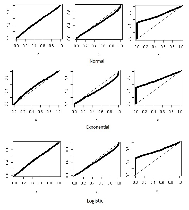
Figure 1: The Q-Q plot for the p-values of the proposed test statistic based on the EAR algorithm (first column), and those proposed by Baklizi (2009) (second column) and Liu et al. (2009) (the third column), respectively for the normal distribution when $H_{0}:\mu=0$ and the exponential and logistic distributions for $H_{0}:\mu=1$.

5 Real data application

In this section, we use a data set containing the birth weight and seven-month weight of 224 lambs along with the mother’s weight at time of mating, collected at the Research Farm of Ataturk University, Erzurum, Turkey. Jafari Jozani and Johnson (2012) as well as Ozturk and Jafari Jozani (2014) used this data set to study the performance of ranked set sampling in estimating the mean, the total values and quantiles of the seven-month weight of these lambs. The measurement of the weight of young sheep is usually labor intensive due to their active nature, and measurement errors can be inflated due to this activity. However, one can easily rank a small number of lambs based on their birth weights or their mother’s weights to perform a ranked set sampling design hoping that the RSS sample results in a more representative sample from the whole population. Here, we treat these 224 records as our population, with the goal of a testing hypothesis problem about the mean of the weight distribution of these 224 lambs at seven-month. We consider both perfect and imperfect ranking cases. For the perfect ranking scenario, ranking is done based on the weight of lambs at seven-month. For the imperfect ranking, we consider two cases. In the first case (Imperfect 1), ranking is done based on the the birth weight of the lambs. The Kendall’s $\tau$ between the seven-month weight and the birth weight is 0.64. In the second case (Imperfect 2), we perform the ranking process based on the mother’s weight at time of mating which results in a small Kendal’s $\tau$ of 0.41 between the lambs weight at seven-month and mother’s weight at the time of mating. Summary statistics for these variables for the underlying population are presented in Table 5. Figure 2 shows the histogram of the seven-month weight of these lambs with a kernel density estimator of their weight distribution. We also present the scatter plots of the birth weight and mother’s weight of these lambs against their weight at seven-months. We observe that there is a stronger association between the seven-month weight and the birth weight of these lambs. So, we expect to observe a better results under the Imperfect 1 scenario.

Table 5: Summary statistics for the values of the birth weight and seven-month weight of 224 lambs along with the mother’s weight at time of mating, collected at the Research Farm of Ataturk University, Erzurum, Turkey

Variable	Min	$Q_{1}$	Median	Mean	$Q_{3}$	Max	$\sigma^{2}$
Seven-month weight	20.30	25.50	27.90	28.11	31.00	40.50	15.21
Birth weight	2.50	3.87	4.40	4.36	4.80	6.70	0.63
Mother’s weight	42.20	49.68	52.30	52.26	55.10	63.70	19.22

Table 6 presents the results of the analysis for a testing hypothesis problem to test $H_{0}:\mu=28.11$ based on different RSS sampling designs as in Section 4. Based on the obtained $\alpha$-level for each sampling design under the PT and EAR algorithm we observe that our proposed bootstrap test using the ET estimator of the DF shows a satisfactory performance compared with the PT method in both perfect and imperfect ranking scenarios.

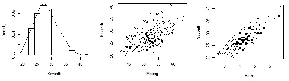
Figure 2: The histogram of the values of seven-month weight of 224 lambs with a kernel density estimator of their weight distribution as well as the scatter plots of the birth weight and mother’s weight of these lambs against their weight at seven-months.

Table 6: The values of the observed $\alpha$-levels for testing $H_{0}:\mu=28.11$ for the weight distribution of a population of 224 lambs based on different perfect and imperfect RSS design using the PT and EAR algorithm.

	Method	$D_{1}$	$D_{2}$	$D_{3}$	$D_{4}$	$D_{5}$
Perfect Ranking	PT	0.062	0.094	0.085	0.076	0.083
	EAR	0.055	0.052	0.044	0.046	0.047
Imperfect 1	PT	0.064	0.082	0.091	0.087	0.094
	EAR	0.048	0.047	0.052	0.047	0.045
Imperfect 2	PT	0.065	0.090	0.086	0.086	0.091
	EAR	0.048	0.042	0.051	0.043	0.046

6 Concluding Remarks

We propose nonparametric estimators of the cumulative distribution of a continuous random variable using the ET empirical likelihood method based on ranked set sampling designs. The ET DF estimators are used to construct new resampling techniques for URSS data. We study different properties of the proposed algorithms. For a hypothesis testing problem, we show that the bootstrap test based on exponential tilted estimators exhibit a small bias of order $O(n^{-1})$, which is a very desirable property. We compared the performance of our proposed techniques with those based on empirical likelihood. The latter are developed under the balanced RSS assumption and they are not applicable for URSS situation. The results of the simulation studies as well as a real data application show that the method based on ET estimators of the DF perform very well even for moderate or small sample sizes.

References

- [1] Ahn, S., Lim, J., & Wang, X. (2014). The Student’st approximation to distributions of pivotal statistics from ranked set samples. Journal of the Korean Statistical Society, 43(4), 643-652.
- [2] Amiri, S. and Jafari Jozani, M., Modarres, R. (2014). Resampling Unbalanced Ranked Set Sampling with application in Testing Hypothesis about the population mean. Journal of Agricultural, Biological, and Environmental Statistics, 19, 1–17.
- [3] Baklizi, A. (2009). Empirical likelihood intervals for the population mean and quantiles based on balanced ranked set samples. Statistical Methods and Applications, 18, 4, 483-505.
- [4] Chaudhuri, S. and Ghosh, M. (2011). Empirical likelihood for small area estimation. Biometrika, Vol. 98, Issue 2, 473-480.
- [5] Chen, Z., Bai, Z. and Sinha, B.K. (2004). Ranked set sampling: theory and applications. Springer-Verlag, New York.
- [6] Davison, A.C. and Hinkley, D.V. (1997). Bootstrap Methods and their Application. Cambridge University Press, Cambridge.
- [7] DiCiccio, T. J., and Romano, J. P. (1990). Nonparametric confidence limits by resampling methods and least favourable families. Internat. Statist. Rev., 58, 59–76.
- [8] Efron, B. (1981). Nonparametric standard errors and confidence intervals (with discussion). Can. J. Statist., 9 , 139–172.
- [9] Efron, B. and Tibshirani, R. (1993). An introduction to bootstrap. Chapman & Hall, New York.
- [10] Feuerveger. A., Robinson, J. and Wong, A. (1999). On the relative accuracy of certain bootstrap procedures. Can. J. Statist. 27. 225–236.
- [11] Frey, J., Ozturk, O. & Deshpande, J.V. (2007). Nonparametric tests for perfect judgment rankings. J. Amer. Statist. Assoc. 102, 708-717.
- [12] Frey, J., & Wang, L. (2013). Most powerful rank tests for perfect rankings. Computational Statistics & Data Analysis, 60, 157-168.
- [13] Hall, P. and Wilson, S.R. (1991). Two guidelines for bootstrap hypothesis testing. Biometrics, 47, 757–762.
- [14] Hall, P. (1992). The Bootstrap and Edgeworth Expansion. New York: Springer-Verlag.
- [15] Jafari Jozani, M. and Johnson, B. C. (2012). Randomized nomination sampling for finite populations. Journal of Statistical Planning and Inference, 142, 2103–2115.
- [16] Kim, J. K. (2010). Calibration estimation using exponential tilting in sample surveys. Survey Methodology, 36(2), 145-155.
- [17] Kostov, P. (2012). Empirical likelihood estimation of the spatial quantile regression. Journal of Geographical Systems, Volume 15, Issue 1, 51-69.
- [18] Li, T. & Balakrishnan, N. (2008). Some simple nonparametric methods to test for perfect ranking in ranked set sampling. J. Statist. Plann. Inference, 138, 1325-338.
- [19] Liu, T., Lin, N., and Zhang, B. (2009). Empirical likelihood for balanced ranked-set sampled data. Science in China Series A: Mathematics, 52(6), 1351–1364.
- [20] Modarres, R., Hui, T.P. and Zhang, G. (2006). Resampling methods for ranked set samples. Computational Statistics & Data Analysis, 51, 1039–1050.
- [21] Owen, A. B. (2001). Empirical Likelihood, Chapman and Hall/CRC.
- [22] Ozturk, O. and Jafari Jozani, M. (2014). Inclusion probabilities in partially rank ordered set sampling. Computational Statistics & Data Analysis, 69, 122–132.
- [23] Patil, G. P., Sinha, A. K. and Taillie, C. (1999). Ranked set sampling: a bibliography. Environmental and Ecological Statistics, 6, 91–98.
- [24] Schennach, S. M. (2005). Bayesian Exponentially-Tilted Empirical Likelihood. Biometrika, 92, 31-46.
- [25] Schennach, S. M. (2007). Point estimation with exponentially tilted empirical likelihood. Annals of Statistics, Vol. 35, No. 2, 634-672.
- [26] Stokes, S. L., and Sager, T. W. (1988). Characterization of a ranked-set sample with application to estimating distribution functions. Journal of the American Statistical Association, 83(402), 374-381.
- [27] Vock, M. & Balakrishnan, N. (2011). A Jonckheere-Terpstra-type test for perfect ranking in balanced ranked set sampling. J. Statist. Plann. Infer. 141, 624-630.
- [28] Wolfe, D. A. (2012). Ranked set sampling: its relevance and impact on statistical inference. International Scholarly Research Notices.