Robust preconditioners for PDE-constrained optimization with limited observations
Kent-Andre Mardal, Bjørn Fredrik Nielsen and Magne Nordaas
Kent-Andre Mardal, Center for Biomedical Computing, Simula Research Laboratory; Department of Mathematics, University of Oslo, Norway. Email: kent-and@simula.noBjørn Fredrik Nielsen, Department of Mathematical Sciences and Technology,
Norwegian University of Life Sciences, Norway; Simula Research Laboratory;
Center for Cardiological Innovation, Oslo University Hospital.
Email: bjorn.f.nielsen@nmbu.noMagne Nordaas, Center for Biomedical Computing, Simula Research Laboratory. Email: magneano@simula.no
Abstract
Regularization robust preconditioners for PDE-constrained
optimization problems have been successfully developed. These
methods, however, typically assume that observation data is
available throughout the entire domain of the state equation. For
many inverse problems, this is an unrealistic assumption. In this
paper we propose and analyze preconditioners for PDE-constrained
optimization problems with limited observation data,
e.g. observations are only available at the boundary of the solution
domain. Our methods are robust with respect to both the
regularization parameter and the mesh size. That is, the condition
number of the preconditioned optimality system is uniformly bounded, independently
of the size of these two parameters. We first consider a
prototypical elliptic control problem and thereafter more general
PDE-constrained optimization problems. Our theoretical findings are
illuminated by several numerical results.
This minimization task is similar to the standard example considered in PDE-constrained
optimization. But instead of assuming that observation data is available everywhere in ,
we consider the case where observations are only given at the boundary of
, that is , see the first term in (1).
For problems of the form (1)-(3), in which
(4)
is replaced by
(5)
very efficient preconditioners have been developed for the associated
KKT system. In fact, by employing proper -dependent scalings
of the involved Hilbert spaces [10], or by using a Schur
complement approach [9], methods that are robust with respect
to the size of the regularization parameter have been
developed.
More specifically, the condition number of the preconditioned optimality system is
small and bounded independently of
and the mesh size . This ensures good performance for suitable
Krylov subspace methods, e.g. the minimum residual method (Minres),
independently of both parameters.
These techniques have been
extended to handle time dependent problems [8] and
PDE-constrained optimization with Stokes equations [12], but
the rigorous analysis of -independent bounds always requires
that observations are available throughout all of .
For cases with limited observations, for example with cost-functionals
of the form (4), efficient preconditioners are also available for a
rather large class of PDE-constrained optimization problems, see
[7, 6]. But these techniques do not yield convergence rates, for
the preconditioned KKT-system, that are completely robust with respect
to the size of the regularization parameter . Instead, the number
of preconditioned Minres iterations grows logarithmically111In
[7, 6] it is proved that the number of needed preconditioned
Minres iterations cannot grow faster than
Furthermore, in [7]
it is explained why iterations counts of the kind (6) often
will occur in practice. with respect to the size of , as :
(6)
According to the numerical experiments presented in [7], the size of may become
significant. More specifically, for problems with simple elliptic state equations
posed on rectangles. Thus, for small values of , Minres may require rather many iterations
to converge - even though the growth in iteration numbers is only logarithmically.
In practice, observations are rarely available throughout the entire
domain of the state equation. On the contrary, the purpose of solving
an inverse problem is typically to use data recorded at the surface of
an object to compute internal properties of that object: Impedance
tomography, the inverse problem of electrocardiography (ECG),
computerized tomography (CT), etc. This fact, combined with the
discussion above, motivate the need for further improving numerical
methods for solving KKT systems arising in connection with
PDE-constrained optimization.
This paper is organized as follows. In the next section we derive the
KKT system associated with the model problem (1)-(3). Our
robust preconditioner is presented in Section
3, along with a number of numerical
experiments. Sections 4-5 contain our
analysis, and the method is generalized in Sections
6-7. Section 8
provides a discussion of our findings, including their limitations.
2 KKT system
Consider the PDE (3) with the boundary condition (3). A
solution to this elliptic PDE, with source term , is
known to have improved regularity, i.e. , for
some , with depending on the domain . In the remainder
of this paper we assume that has full regularity, i.e. . This is known to hold if is convex or if
is , see e.g. [2, 4].
When solutions to (3) exhibit this improved regularity, we can
write the problem on the non-standard variational form: Find such
that
(7)
where
equipped with the inner product
(8)
Here denotes the Hessian of , and the second identity is due to the boundary condition
imposed on the space .
We will see below that, in order to design a regularization robust
preconditioner for (1)-(3), it is convenient to express the
state equation in the form (7), instead of employing integration
by parts/Green’s formula to write it on the standard self-adjoint form.
with , and .
From the first order optimality conditions
we obtain the optimality system: Determine
such that
(11)
(12)
(13)
3 Numerical experiments
Prior to analyzing our model problem, we will consider some numerical experiments.
Discretization of (11)-(13) yields an algebraic system of the form
(14)
where
•
is a mass matrix,
•
is a mass matrix associated with the boundary of .
•
is a matrix that arise upon discretization of
the operator . Since we write the state equation on a non self-adjoint
form, will not be the usual sum of the stiffness and mass
matrices. Instead, equation (7) is discretized with subspaces
of and .
In the current numerical experiments, we employ the Bogner-Fox-Schmit
(BFS) rectangle for discretizing the state variable .
That is, the finite element field consists of bicubic polynomials
that are continuous, have continuous first order derivatives and mixed
second order derivatives at each vertex of the mesh. BFS elements are
on rectangles and therefore -conforming. The control
and Lagrange multiplier are discretized with discontinuous bicubic
elements.
We propose to precondition (14) with the block-diagonal matrix
(15)
where results from a discretization of the bilinear form on :
(16)
In the experiments presented below, we used this bilinear form to
construct a multigrid approximation of .
Remark
The bilinear form (16) is equivalent to the inner product on
. The additional term stems from our choice of implementing a
multigrid algorithm for the bilinear form associated with the operator
. Indeed, the bilinear
form can be seen to
coincide with the variational form associated with the fourth order problem
To limit the technical complexity of the implementation, we considered
the problem (1)-(3) on the unit square in two dimensions.
The experiments were implemented in Python and SciPy. The meshes were
uniform rectangular, with the coarsest level for the multigrid solver
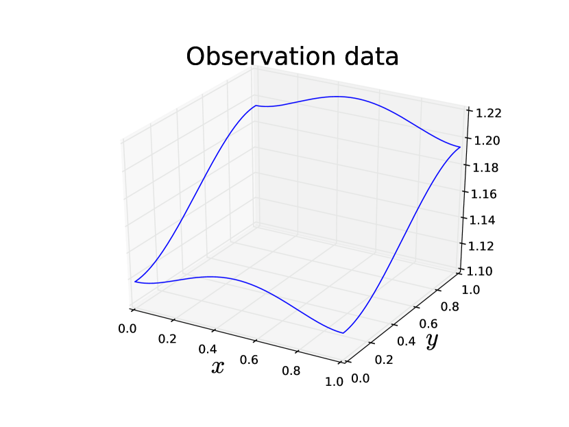
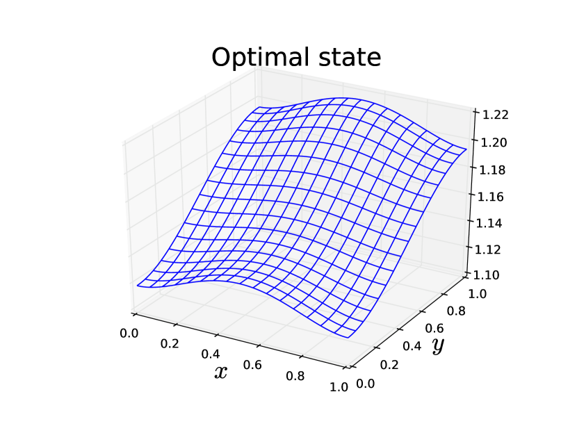
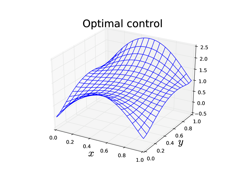
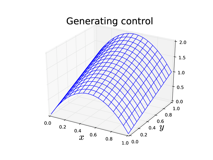
consisting of rectangles. Figure 1 shows an example of a
solution of the optimality system (14).
(a)Observation data . The forward model was solved for
the control shown in (1(d)), but only the
boundary values can be observed.
(b)Computed optimal state based on the observation data
shown in (1(a))
(c)Computed optimal control based on the observation
data in (1(a))
(d)The “true” control function used to generate the observation data in
(1(a)).
Figure 1: An example of a solution of (14). The
observation data was generated with the forward model, using
the “true” control shown in panel
(1(d)). Solutions to the unregularized problem are
non-unique, and the generating control cannot be (exactly) recovered. The
figures were generated with mesh parameter
and regularization parameter .
3.1 Eigenvalues
Let us first consider the exact preconditioner defined in (15).
If is a good preconditioner for the
discrete optimality system (14), then the spectral condition
number of should be small and bounded, independently
of the size of both the regularization parameter and the discretization
parameter .
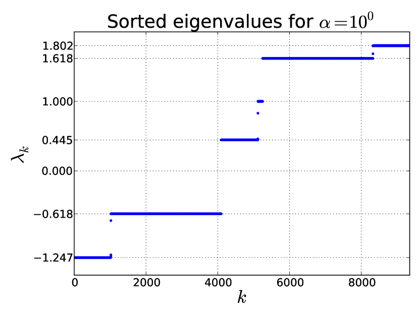
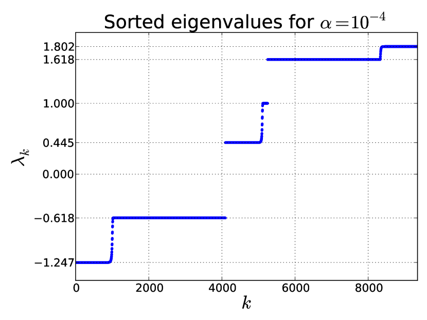
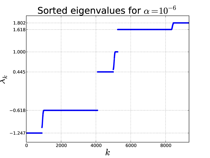
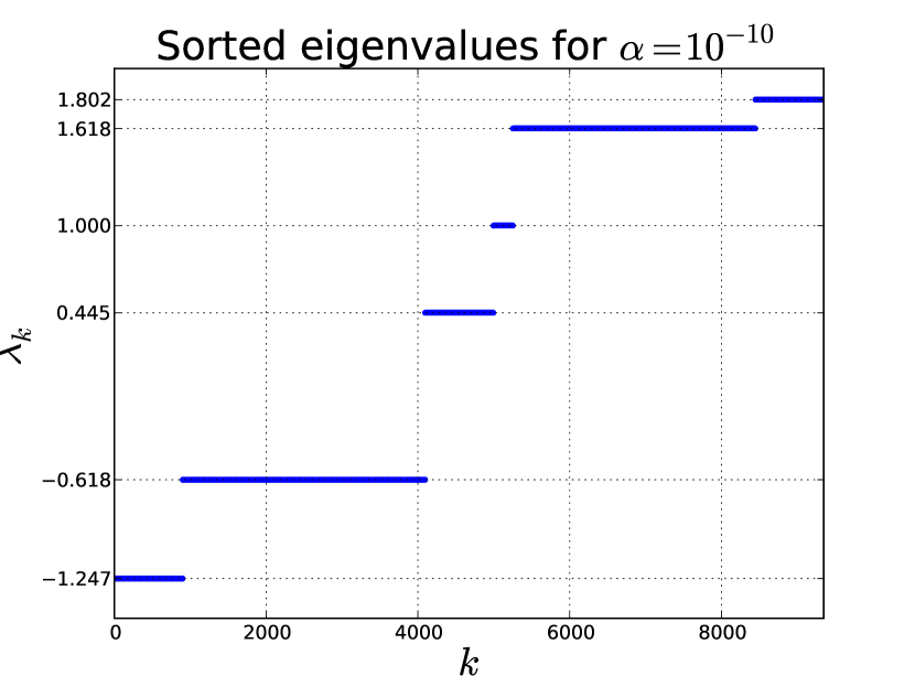
The eigenvalues of this preconditioned system were
computed by solving the generalized eigenvalue problem
We found that the absolute value of the eigenvalues were bounded, with
uniformly in and . This yields a uniform condition number
. The spectra of the preconditioned
systems are pictured in Figure 2 for some
choices of . The spectra are clearly divided into three
bounded intervals, and the eigenvalues are more clustered for and for very small .
(a)
(b)
(c)
(d)
Figure 2: Spectrum of for different regularization
parameters . The discretization parameter
was for all figures.
3.2 Efficient preconditioning
In practice, the action of is replaced with a less
computationally expensive operation . Note that
has a block structure, and that computationally efficient approximations can be
constructed for the individual blocks. Specifically,
is constructed by employing
•
1 multigrid V-cycle for the (2,2) block of , containing a symmetric block Gauss-Seidel
smoother where the blocks contain the matrix entries corresponding to all degrees of freedom associate with a vertex in the mesh
(see [11] for a theoretical analysis of the method).
•
2 symmetric Gauss-Seidel iterations for the (1,1) and (3,3) blocks.
We estimated condition numbers of the individual blocks of preconditioned
with their respective approximations. The results are reported in Tables
2 and 2. A slight deterioration in the
performance of the multigrid cycle can be seen for very small values of
.
Iterations
1
2
3
()
1.931
1.303
1.126
Table 1: Condition numbers of preconditioned with symmetric
Gauss-Seidel iterations.
\
1.130
1.136
1.140
1.129
1.135
1.139
1.237
1.150
1.149
1.252
1.259
1.253
Table 2: Estimated condition numbers of
preconditioned with one V-cycle multigrid iteration.
3.3 Iteration numbers
To verify that also is an effective
preconditioner for , we applied the Minres scheme to the system
For the results presented in Table
3, the Minres iteration
process was stopped as soon as
(17)
which is the standard termination criterion for the preconditioned
Minres scheme, provided that the preconditioner is SPD. A random
initial guess was used, and the tolerance was set to .
\
1
53(4.33)
53(4.36)
53(4.36)
53(4.36)
57(4.31)
57(4.34)
57(4.35)
57(4.35)
75(4.31)
72(4.34)
70(4.35)
68(4.35)
79(4.31)
79(4.34)
77(4.35)
73(4.35)
81(4.30)
81(4.33)
79(4.35)
77(4.35)
82(4.33)
81(4.33)
79(4.35)
79(4.35)
81(4.35)
79(4.36)
79(4.35)
81(4.35)
70(4.35)
81(4.37)
81(4.36)
79(4.35)
62(4.36)
70(4.36)
79(4.36)
81(4.36)
62(4.36)
64(4.37)
68(4.37)
78(4.36)
62(4.36)
63(4.36)
64(4.37)
67(4.37)
Table 3: Number of preconditioned Minres iterations needed to solve the optimality system to a relative error tolerance .
Estimated condition numbers in parentheses, computed from conjugate gradient iterations on the normal equations for the preconditioned optimality system.
4 Analysis of the KKT system
Recall that our optimality system reads:
with unknowns , and .
We may write this KKT system in the form:
Determine
such that
(18)
where
(19)
(20)
(21)
(22)
and the notation ”′” is used to denote dual operators and dual spaces.
In the rest of this paper, the symbols , and will represent the mappings
defined in (19), (20) and (22), respectively, and not (the associated) matrices, as
was the case in Section 3. (We believe that this mild ambiguity improves the readability of the present text).
By using standard techniques for saddle point problems, one can show
that the system (18) satisfies the Brezzi conditions [1],
provided that . Therefore, for every , this
set of equations has a unique solution. Nevertheless, if the standard
norms of and are employed in the analysis, then the
constants in the Brezzi conditions will depend on . More
specifically, the constant in the coercivity condition will be of
order , and thus becomes very small for . This property is consistent with the ill posed nature of
(1)-(3) for , and makes it difficult to design
robust preconditioners for the algebraic system associated
with (18).
Similar to the approach used in [10, 5, 6], we will now introduce
weighted Hilbert spaces. The weights are constructed such that the
constants appearing in the Brezzi conditions are independent of
. Thereafter, in Section 5, we will show
how these scaled Hilbert spaces can be combined with simple maps to
design robust preconditioners for our model problem.
4.1 Weighted norms
Consider the -weighted norms:
(23)
(24)
(25)
applied to the control , the state and the dual/Lagrange-multiplier , respectively. Note that these norms become
“meaningless” for , but are well defined for positive .
4.2 Brezzi conditions
We will now analyze the properties of
defined in (18).
More specifically, we will show that the Brezzi conditions are satisfied
with constants that do not depend on the size of the regularization parameter .
Note that we use the scaled Hilbert norms (23)-(25).
Lemma 4.1
For all , the following “inf-sup” condition holds:
Proof
Note that and contain the same functions, provided that .
Let be arbitrary.
By choosing and we find that
Since was arbitrary, this completes the proof.
Expressed in terms of the operators that constitute
, Lemma 4.1 takes the form
Recall that we decided to write our state equation (3)-(3)
on the non-standard variational form (7). Throughout this paper
we assume that problem (3)-(3) admits a unique solution for
every , and that
(26)
This assumption is valid if is convex or if has a
boundary, see e.g. [2, 4]. Inequality
(26) is a key ingredient of the proof of our next lemma.
Lemma 4.2
There exists a constant , which is independent of , such that
see the discussion of (26). Let , and it follows that
This result may also be written in the form
for all satisfying
where , and are the operators defined in (19), (20) and (22), respectively.
4.3 Boundedness
Having established that the Brezzi conditions hold, with constants that are
independent of , we next explore the boundedness of .
Lemma 4.3
for all .
Proof
Recall the definitions (19) and (20) of and , respectively.
Since
we find, by employing the Cauchy-Schwarz inequality, that
Lemma 4.4
for all , .
Proof
Again, we note that
From the definitions of and , see (19) and (22), and
the Cauchy-Schwarz inequality, it follows that
For the last equality, recall from (8) that
for all .
4.4 Isomorphism
We have verified that the Brezzi conditions hold, and that is
a bounded operator. Moreover, all constants appearing in the inequalities expressing
these properties are independent of the regularization parameter .
Let
(28)
(29)
Theorem 4.5
The operator , defined in (18),
is bounded and continuously invertible for in the sense that for all nonzero ,
(30)
for some positive constants and that are independent of . In particular,
Proof
This result follows from Lemma 4.1, Lemma 4.2,
Lemma 4.3, Lemma 4.4 and Brezzi theory for
saddle point problems, see [1].
4.5 Estimates for the discretized problem
The stability properties (30) is not
necessarily inherited by discretizations. However, the structure used
to prove the so-called “inf-sup condition” in Lemma
4.1 is preserved in the discrete system provided that
the same discretization is employed for the control and the Lagrange
multiplier. Furthermore, the boundedness properties, Lemma
4.3 and Lemma 4.4, certainly also hold for
conforming discretizations.
It remains to adress the coercivity condition, Lemma
4.2, for the discretized problem. We consider finite
dimensional subspaces and . For certain choices of and , the estimate of Lemma
4.2 carries over to the finite-dimensional setting.
Lemma 4.6
Assume and
, such that .
Then
(31)
for all such that
(32)
Proof
Assume that , and that
(32) holds for . Then , and (32) implies . Therefore, satisfies (27) and the estimate
(31) follows from Lemma
4.2.
If the discretization is chosen such that Lemma
4.6 is satisfied, then the estimates
(30) carries over to discretized system.
More precisely, we have
(33)
where , equipped with the
inner prdocut of , and is discrete counterpart to ,
defined by setting for
all .
If the state is discretized with -conforming bicubic
Bogner-Fox-Schmit rectangles, as in Section
3, then Lemma 4.6 is
satisfied if the control and Lagrange multiplier is discretized with
discontinuous bicubic elements on the same mesh. For triangular
meshes, one could choose Argyris triangles for the state variable and
piecewise quintic polynomials for the control and Lagrange multiplier
variables.
We remark that Lemma 4.6 provides a sufficient,
but not necessary criterion for stability of the discrete problem, and
usually may imply far more degrees of freedom in the discrete space
than is actually needed. The usefulness of Lemma
4.6 is that the estimates
(33) can, in principle, always be obtained
by choosing a sufficiently large space for the control and Lagrange
multiplier.
where is sought in a Hilbert space , the right hand side is
in the dual space , and is a self-adjoint continuous mapping
of onto . Iterative methods for linear problems are most
often formulated for operators mapping into itself, and can not
be directly applied to the linear system (34), as described
in [5]. If we want to apply such methods to (34),
then we need to introduce a continuous operator mapping
isomorphically back onto . More precisely, if we have a continuous
operator
then is continuous and has the desired
mapping properties, and if is an isomorphism, the solutions to
(34) coincides with the solutions to the problem
(35)
In this paper we shall consider a preconditioner
if is self-adjoint and positive definite. This implies that
is self-adjoint and positive definite as well, and hence
defines an inner product on by setting
(36)
This inner product has the crucial property of making self-adjoint, in the sense that
(37)
Conversely, given any inner product on on ,
the Riesz-Fréchet theorem provides a self-adjoint positive definite
isomorphism such that (36) and
(37) hold, and we say that is the Riesz operator
induced by . This establishes a one-to-one
correspondence between preconditioners and Riesz operators on .
Since the Riesz operator is an isometric isomorphism, the operator
norm of coincides with the operator norm of . We formulate
this well-known fact here in a lemma for the sake of self-containedness. We refer to
[5, 3] for a more in-depth discussion of
preconditioning and its relation to Riesz operators.
Lemma 5.1
Let be a Hilbert space, and let be a
self-adjoint isomorphism, and assume that is the Riesz operator
induced by the inner product on , or
equivalently, that the inner product on is defined by the self-adjoint
positive definite isomorphism . Then
is an isomorphism, self-adjoint in the inner product on , with
In particular, the condition number of is given by
Proof
Since is self-adjoint, is
self-adjoint with respect to the inner product on . From the
Riesz-Fréchet theorem we have , and we obtain following identity for the operator norm
of .
A similar identity is obtained for the norm of the inverse operator,
We say that a preconditioner for is robust
with respect to the parameter if
is bounded uniformly in . The significance of Lemma
5.1 is that such a robust preconditioner can be
found by identifying (parameter-dependent) norms in which and
are both uniformly bounded.
5.1 Parameter-robust minimum residual method
In Section 4 stability of was shown in the
-dependent norms defined in (23)-(25). The
preconditioner provided by Lemma 5.1 is the
Riesz operator induced by the weighted norms. This operator takes the form
(38)
where is the operator induced by the
inner product, i.e. .
Since is self-adjoint, the
preconditioned operator is self-adjoint in the
inner product on . Consequently we can apply the
minimum residual method (Minres) to the problem
Theorem 5.2
Let be the operator defined in (18) and the operator
defined in (38). Then there exists an upper bound,
independent of , for the convergence rate of Minres applied to the preconditioned system
In particular there exists an upper bound, independent of , for the number of iterations
needed to reach the stopping criterion (17).
Proof
A crude upper bound for the convergence rate (more precisely, the
two-step convergence rate) of Minres is given by
where is the condition number of ,
see e.g. [5]. From Lemma 5.1 and
(30) we determine that is bounded
independently of , with
(39)
In practical applications, the operator will be replaced with a
less computationally expensive approximation . Ideally
will be spectrally equivalent to , in the sense
that the condition number of is bounded,
independently of . Then the preconditioned system reads
and the upper bound for the convergence rate is determined by the conditioned number
.
Remark
In this paper we only consider the minimum residual method, and we
therefore require that the preconditioner is self-adjoint and positive
definite. More generally, if other Krylov subspace methods are
to be applied to (18), then preconditioners lacking symmetry or
definiteness may be considered.
We mention in particular that a preconditioned conjugate gradient
method for problems similar to (18) was proposed in [10],
based on a clever choice of inner product.
6 Generalization
Is our technique applicable to other problems than (1)-(3)?
We will now briefly explore this issue, and show that the preconditioning scheme
derived above yields robust methods for a class of problems.
The scaling (23)-(25) was also investigated in
[6], but for a family of abstract problems posed in terms of
Hilbert spaces. More specifically, for general PDE-constrained
optimization problems, subject to Tikhonov regularization, and with
linear state equations. But in [6] no assumptions about the
control, state or observation spaces were made, except that they were
Hilbert spaces. Under these circumstances, it was proved that the
coercivity and the boundedness, of the operator associated with the
KKT system, hold with -independent constants. Nevertheless, in
this general setting, the inf-sup condition involved an
-dependent constant, which, eventually, yielded theoretical
iteration bounds of order
for Minres.
In the present paper we were able to prove an -robust
inf-sup condition for the model problem (1)-(3). This is possible because both the
control and the dual/Lagrange-multiplier belong to .
From a more general perspective, it turns out that this is the
property that must be fulfilled in order for our approach to be
successful: The control space and the dual space, associated with the
state equation, must coincide. This will usually lead to additional
regularity requirements for the state space.
Motivated by this discussion, let us consider an abstract problem of the form:
(40)
subject to
(41)
Here,
•
is the dual and control space,
•
is the state space,
•
is the observation space,
•
, and are Hilbert spaces.
Let us assume that
•
is a continuous linear operator with
closed range. In particular, there is a constant such that for all ,
•
is linear and bounded, and invertible on the kernel of .
That is, there is a constant such that for all ,
It then follows that the KKT system associated with
(40)-(41) is well-posed for every :
Determine such that
(42)
where
(43)
(44)
(45)
Note that, compared with (14), the boundary observation matrix has been
replaced with the general observation operator in (42).
We introduce scaled norms as follows.
We first show that is indeed a norm on when assumptions • ‣ 6 and • ‣ 6 hold.
It suffices to show that is a norm equivalent to
when . We have
(46)
and letting denote the orthogonal projection of onto ,
(47)
Here the last inequality follows from and assumption • ‣ 6.
We set . As in
Section 4, can be shown to be
an isomorphism, with parameter-independent estimates obtained in the
weighted norms.
Theorem 6.1
There exists positive constants and ,
independent of , such that for all
nonzero ,
(48)
We omit the full proof, which is analogous to that of Theorem
4.5. The crucial part is the “inf-sup condition” of Lemma 4.1, which is
easily shown to hold in the abstract setting:
The coercivity condition of Lemma 4.2 naturally holds
in the prescribed norm on , since for
such that ,
Note that the weighted norm now depends on , and as consequence,
the estimates become -independent. In fact, we obtain bounds for
the constants and which are independent of as well as the
operators appearing in (40)-(41). This is postponed to
the next section, where sharp estimates are obtained for
(48).
With the estimates (48), Lemma
5.1 provides a preconditioner for the operator
, given as
(49)
The condition number of will be bounded independently of
. It is, however, not clear how to find a computationally
efficient approximation of in the abstract setting of
(40)-(41).
Example 1
The problem (1)-(3) fits in the abstract framework
presented in this section when we assume that the state has
regularity. We set , , , and
is a trace operator, see (44). Since is a continuous
isomorphism, assumptions • ‣ 6 and • ‣ 6 are both valid. The inner
product on takes the form
where denotes the Hessian of , and the last equality
follows from the boundary condition imposed on . The resulting preconditioner is the one that
was used in the numerical experiments, detailed in Section
3, and it is spectrally equivalent to the
preconditioner defined in (38).
Example 2
Let , , and be as in Example 1, but let us
set . Now has non-trivial kernel, consisting of the
a.e. constant functions, and for constant we have
Since assumptions • ‣ 6 and • ‣ 6 are valid, the optimality system
is still well-posed. In this case the inner product on is
given by
Example 3
Let us consider the “prototype” problem:
subject to
Note that we here consider the case in which observation data is assumed
to be available throughout the entire domain of the state
equation.
If the usual variational form of the PDE is used, i.e.,
(50)
then the control space equals , whereas the dual
space is . The preconditioning strategy presented in this
section is therefore not applicable.
If instead we can assume -regularity, we can use the variational form
(51)
Now, the control and dual spaces both equal . The methodology
presented in this section can thus be applied, and a robust
preconditioner is obtained. Compared with the preconditioner for the
problem with boundary observations only, see Section
5, equation (38), the only change is
the replacement of , in the block of with
.
We remark that in [10] and [9], parameter-robust
preconditioners were proposed for the “prototype” problem, using the
standard variational formulation (50) of the PDE. Those
methods do not require improved regularity for the state
space. Instead, they require that observations are available
throughout the computational domain.
7 Eigenvalue analysis
In Section 6 it was shown that the condition
number of , with defined in (42) and
defined in (49), can be bounded independently of
, as well as independently of the operators appearing in
(40)-(41). Moreover, the numerical experiments indicate
that the eigenvalues are contained in three intervals, independently of
the regularization parameter , see Figure 2. In this
section we detail the structure of the spectrum of the preconditioned
system considered in Section 6, and we obtain sharp
estimates for the constants appearing in Theorem 6.1.
We consider self-adjoint linear operators
and ,
(52)
where is defined by
(53)
We assume that and are
continuous operators, for some Hilbert spaces and . In addition
we will make use of the following assumptions.
•
is a self-adjoint and positive definite,
•
is positive definite,
•
is self-adjoint and positive semi-definite.
Assumptions • ‣ 7-• ‣ 7 ensure that is a
self-adjoint and positive definite. In particular, assumptions • ‣ 7-• ‣ 7 hold
for as in (42), provided that the assumptions of Section
6 hold. For simplicity, we also assume that that
and are
finite-dimensional operators.
Theorem 7.1
Let , , and be the polynomials
Let and be the roots of and ,
respectively. The spectrum of is contained
within three intervals, determined by the roots of and ,
independently of :
(54)
Consequently, the spectral condition number of is bounded, uniformly in ,
(55)
If has a nontrivial kernel, inequality (55)
becomes an equality.
Proof
Consider the equivalent generalized eigenvalue problem
(62)
We show that (62) admits no nontrivial solutions
unless is as in (54).
Since is a self-adjoint isomorphism, by assumption • ‣ 7, we can
rewrite (62) as the three identities
(63)
(64)
(65)
Assume that is not contained within the three closed intervals
of (54).
Then , and we can use (63)
to eliminate from (65).
(66)
Since is nonzero, we can use (66) to eliminate from (64),
(67)
where the identity (53) was used. By assumption, and
are both nonzero. Moreover, it can be easily seen that and
have the same sign outside of the bounded intervals of
(54). From assumptions • ‣ 7-• ‣ 7, we conclude that
is a self-adjoint definite operator. Then (67)
only admits trivial solutions, hence can not be
an eigenvalue of .
The estimate (55) follows from
(54), noting that . From (67) it
can be seen that the roots of are eigenvalues of
if is nontrivial.
Remark
If , then
is characterized by a bilinear form as in (16):
For discretizations and of such that
, the discretization of coincides with
. This follows from an argument similar to that in
the proof of Lemma 4.6, and as a consequence,
Theorem 7.1 can be applied to the preconditioned discrete
systems considered in Section 3.
8 Discussion
Previously, parameter robust preconditioners for PDE-constrained
optimization problems have been successfully developed, provided that
observation data is available throughout the entire domain of the
state equation. For many important inverse problems, arising in
industry and science, this is an unrealistic requirement. On the
contrary, observation data will typically only be available in
subregions, of the domain of the state variable, or at the boundary of
this domain. We have therefore explored the
possibility for also constructing robust preconditioners for
PDE-constrained optimization problems with limited observation data.
For an elliptic control problem, with boundary observations only, we
have developed a regularization robust preconditioner for the
associated KKT system. Consequently, the number of Minres iterations
required to solve the problem is bounded independently of both
regularization parameter and the mesh size . In order to
achieve this, it was necessary to write the elliptic state equation on
a non-standard, and non-self-adjoint, variational form. If this
approach is employed, then the control and the Lagrange multiplier
will belong to the same Hilbert space, which leads
to extra regularity requirements for the state. This fact makes it possible to
construct parameter weighted metrics such that the constants
appearing in the Brezzi conditions, as well as the
constants in the inequalities expressing the boundedness of the KKT
system, are independent of and . Consequently, the
spectrum of the preconditioned KKT system is uniformly bounded with
respect to and , which is ideal for the Minres scheme.
These properties were illuminated through a series of numerical experiments,
and the preconditioned Minres scheme handled our model problem excellently.
The use of a non-self-adjoint form of the elliptic state equation
leads to additional challenges for constructing discretization schemes
and suitable multigrid methods. More specifically, it becomes
necessary to implement a FE space approximating . We accomplished
this by a discretization that is conforming in . The method
employed does, however, have strong restrictions on the mesh, which
seemingly must be composed of rectangles.
References
[1]
F. Brezzi.
On the existence, uniqueness and approximation of saddle–point
problems arising from Lagrangian multipliers.
RAIRO numerical analysis, 8:129–151, 1974.
[2]
P. Grisvard.
Elliptic problems in nonsmooth domains.
Pitman, Boston, 1985.
[3]
A. Günnel, R. Herzog, and E. Sachs.
A note on preconditioners and scalar products in Krylov subspace
methods for self-adjoint problems in Hilbert space.
Electronic Transactions on Numerical Analysis, 41:13–20, 2014.
[4]
W. Hackbusch.
Elliptic differential equations. Theory and numerical
treatment.
Springer-Verlag, 1992.
[5]
K. A. Mardal and R. Winther.
Preconditioning discretizations of systems of partial differential
equations.
Numerical Linear Algebra with Applications, 18(1):1–40, 2011.
[6]
B. F. Nielsen and K. A. Mardal.
Efficient preconditioners for optimality systems arising in
connection with inverse problems.
SIAM Journal on Control and Optimization, 48(8), 2010.
[7]
B. F. Nielsen and K. A. Mardal.
Analysis of the Minimal Residual Method applied to ill-posed
optimality systems.
SIAM Journal on Scientific Computing, 35(2):A785–A814, 2013.
[8]
J. W. Pearson, M. Stoll, and A. J. Wathen.
Regularization-robust preconditioners for time-dependent
PDE-constrained optimization problems.
SIAM Journal on Matrix Analysis and Applications,
33:1126–1152, 2012.
[9]
J. W. Pearson and A. J. Wathen.
A new approximation of the Schur complement in preconditioners for
PDE-constrained optimization.
Numerical Linear Algebra with Applications, 19:816–829, 2012.
[10]
J. Schöberl and W. Zulehner.
Symmetric indefinite preconditioners for saddle point problems with
applications to PDE-constrained optimization problems.
SIAM Journal on Matrix Analysis and Applications,
29(3):752–773, 2007.
[11]
X. Zhang.
Multilevel schwarz methods for the biharmonic dirichlet problem.
SIAM Journal on Scientific Computing, 15(3):621–644, 1994.
[12]
W. Zulehner.
Nonstandard norms and robust estimates for saddle point problems.
SIAM Journal on Matrix Analysis and Applications, 32:536–560,
2011.