Finite size corrections in random matrix theory and Odlyzko’s data set for the Riemann zeros

Abstract.

Odlyzko has computed a data set listing more than $10^{9}$ successive Riemann zeros, starting at a zero number beyond $10^{23}$. The data set relates to random matrix theory since, according to the Montgomery-Odlyzko law, the statistical properties of the large Riemann zeros agree with the statistical properties of the eigenvalues of large random Hermitian matrices. Moreover, Keating and Snaith, and then Bogomolny and collaborators, have used $N\times N$ random unitary matrices to analyse deviations from this law. We contribute to this line of study in two ways. First, we point out that a natural process to apply to the data set is to thin it by deleting each member independently with some specified probability, and we proceed to compute empirical two-point correlation functions and nearest neighbour spacings in this setting. Second, we show how to characterise the order $1/N^{2}$ correction term to the spacing distribution for random unitary matrices in terms of a second order differential equation with coefficients that are Painlevé transcendents, and where the thinning parameter appears only in the boundary condition. This equation can be solved numerically using a power series method. Comparison with the Riemann zero data shows accurate agreement.

1. Introduction

The celebrated Riemann hypothesis asserts that all the non-trivial zeros of the Riemann zeta function $\zeta(s)$ are on the so-called critical line, Re$\,s=1/2$. We will refer to zeros of $\zeta(s)$ on the critical line as Riemann zeros, and restrict attention to those in the upper half plane — those in the lower half plane are obtained by complex conjugation. There is an intriguing relationship between the Riemann zeros and random matrix theory. It originates from the viewpoint that the Riemann zeros, for distances far up the critical line, are best considered in a statistical sense rather than as a deterministic sequence. The first step in a statistical analysis is to scale the sequence so that locally the density of the zeros far up the critical line is unity. This is straightforward from knowledge of the fact that at position ${1\over 2}+iE$ along the critical line, and with $E\gg 1$, the density ($\bar{\rho}$ say) is given by [55, pg. 280]

$$\bar{\rho}=\frac{1}{2\pi}\log\Big{(}{E\over 2\pi e}\Big{)}+{\rm O}\Big{(}{\log E\over E}\Big{)}.$$ (1.1)

Montgomery [44, 45] made a study of the density of the scaled zeros about a fixed zero, with the latter averaged over some window of size $\Delta E$, with $\Delta E\ll E$. This quantity, referred to as the two-point correlation function, is probed by computing the average value of a test function $f(E-E_{0})$, with $E_{0}$ corresponding to the fixed zero. Subject to the technical assumption that the class of test function used has Fourier transform supported on $|k|<2\pi$, the limiting two-point correlation function was proved to be equal to

$$\lim_{N\to\infty}\rho^{\mathrm{R}}_{(2)}(E,E+s)=1-\Big{(}{\sin\pi s\over\pi s}\Big{)}^{2},$$ (1.2)

where the superscript ‘R’ denotes that this quantity pertains to the Riemann zeros data. On the other hand, let $X$ be an $N\times N$ random matrix with standard complex Gaussian entries, and form the Hermitian matrix ${1\over 2}(X+X^{\dagger})$ — the set of such matrices specifies the Gaussian Unitary Ensemble (GUE). After normalisation so that the eigenvalues in the bulk of the spectrum have unit density, the $N\to\infty$ form of the two-point correlation function is precisely (1.2); see e.g. [27, Prop. 7.1.1].

This coincidence, first observed by Dyson (see e.g. [12, pg. 159]), is in keeping with and extends the so-called Hilbert–Pólya conjecture [56] that the Riemann zeros correspond to the eigenvalues of some unbounded self-adjoint operator. Considerations in quantum chaos (see e.g. [34, 5]) give evidence that generically the large eigenvalues of such operators have local statistics coinciding with the eigenvalues of large random Hermitian matrices. The latter must be constrained to have real entries should there be a time reversal symmetry. Thus this line of reasoning suggests that asymptotically the Riemann zeros have the same local statistical properties as the large eigenvalues of a chaotic quantum system without time reversal symmetry. This assertion is essentially a statement of what now is called the Montgomery–Odlyzko law or the GUE conjecture; see also [3, 4] the reviews [12, 26], and the thesis [50].

At an analytic level, further evidence for the validity of the law was given by Rudnick and Sarnak [51], who extended Montgomery’s result to the general $k$-point correlation function by obtaining the explicit functional form

$$\det\left[{\sin\pi(x_{j}-x_{l})\over\pi(x_{j}-x_{l})}\right]_{j,l=1,\dots,k},$$ (1.3)

again subject to a constraint on the Fourier transform of the class of test functions involved; see the recent work [22] for some refinements. By use of a conjecture of Hardy and Littlewood relating to the pair correlation of prime numbers, and also at the expense of introducing some non-rigorous working, Bogomolny and Keating [9, 10, 11] removed this constraint. The $k$-point correlation (1.3) is precisely that for the eigenvalues of large Hermitian random matrices in the bulk scaling limit; see again [27, Prop. 7.1.1]. At a numerical level, Odlyzko has made high precision computations of the $10^{20}$-th Riemann zero and over 70 million of its neighbours [46], and (later) of the $10^{22}$-nd zero and one billion of its neighbours [47]. (The zeros on the critical line are conventionally numbered in the order of their distance from the real axis, with the first zero at $\mathrm{Im}\,s\approx 14.134725$ [53, A058303].) This data exhibits consistency with random matrix theory for statistical quantities such as the pair correlation function outside the range known rigorously from the work of Montgomery, the distribution of the spacing between neighbouring zeros, the variance of the fluctuation of the number density in an interval etc.; for a popular account of this line of research see [35].

Notwithstanding the extraordinary distance along the critical line achieved in Odlyzko’s calculations, it turns out that finite size corrections to the limiting behaviour occur on the scale of the logarithm of the distance as suggested by (1.1), and thus are of significance in the interpretation of the data from the viewpoint of the random matrix predictions. In addressing the question of the functional form of the finite size corrections from the viewpoint of random matrix theory, Keating and Snaith [39] (see also the review [40] and the later work [21]) were led to a totally unexpected conclusion: the correct model for this purpose is not complex random Hermitian matrices, but rather $N\times N$ random unitary matrices chosen with Haar measure, and $N$ related to $E$ so as to be consistent with (1.1). Random unitary matrices with Haar measure result, for example, by applying the Gram-Schmidt orthonormalisation procedure to a matrix of standard complex Gaussians. The statistical quantities considered in [39] relate to the value distribution of the logarithm of the Riemann zeta function on the critical line, which for random matrices corresponds to the value distribution of the characteristic polynomial. Coram and Diaconis [23] subsequently used the random unitary matrix model to predict the functional form of the covariance between the number of eigenvalues in overlapping intervals of equal size. Following up on [47], where Odlyko studies the difference between the spacing distribution for the Riemann zeros and the corresponding limiting random matrix distribution and writes: “Clearly there is structure in this difference graph, and the challenge is to understand where it comes from”, Bogomolny et al. [8] considered finite size corrections to the spacing distribution for random unitary matrices. While previous studies in random matrix theory gave analytic results relating to the value distribution of the characteristic polynomial [1], there is no existing literature on the analytic calculations of the leading finite size correction to the spacing distribution for random unitary matrices. Here we are referring to the point-wise value of the expected probability density function; there is an existing literature relating to the decay as a function of $N$ of the Kolmogorov distance between the empirical cumulative spacing distribution and its expected large $N$ form [38, 52, 42]. In [8] the corrections were computed using an extrapolation procedure of a determinant expression valid for finite $N$. A primary objective of the present paper is to provide an analytic characterisation of the leading finite size correction to the spacing distribution.

Variants of the nearest neighbour spacing distribution also provide relevant statistical quantities. For example, one could consider spacing distributions between zeros $k$ apart (see e.g. [27, §8.1]), or the distribution of the closest of the left and right neighbours [29]. Another variant is to consider spacing distributions resulting from first thinning the data set by the process of deleting each member independently with probability $(1-\xi)$, $0<\xi<1$, as first considered in random matrix theory by Bohigas and Pato [13]. In both cases the finite size correction to the large $N$ form of the corresponding quantity for the eigenvalues of random unitary matrices can be computed analytically. This is of concrete consequence as we are fortunate enough to have had A. Odlyzko provide us with a data set extending that reported in [47]. Specifically, this data set begins with zero number

$$100,000,000,000,000,985,531,550\approx 10^{23},$$

and this occurs at the point $s=1/2+iE$ in the complex $s$-plane with $E$ equal to

$$13066434408793621120027.3961465854\approx 1.30664344\times 10^{22}.$$

The data set contains a list of slightly more than $10^{9}$ of each of the subsequent Riemann zeros. Thus we are able to compare the analytic forms against the finite corrections exhibited by the Riemann zeros, uninhibited by sampling error.

We begin in Section 2 by considering the two-point correlation. Bogomolny and Keating [11] have derived an explicit formula for this quantity in the case of the Riemann zeros, in the regime that $E$ is large but finite. Subsequently Bogomolny et al. [8] showed how the result of [11] could be expanded for large $E$ to obtain the correction term to the random matrix result (1.1). Moreover, upon (partial) resummation, the correction term was found to be identical in its functional form to the correction term of the scaled large $N$ expansion of the two-point correlation for the eigenvalues of random unitary matrices chosen with Haar measure. After reviewing this result, we compare the empirical form of the two-point correlation as computed from Odlykzko’s data set, and for the data set thinned with parameter $\xi=0.6$, against the theoretical prediction. Very good agreement is found for distances up to approximately one and a half times the average spacing between zeros, after which systematic deviation is observed.

Higher order correlations for random unitary matrices are fully determined by the same function — see (2.1) below — as determines the two-point correlation. Assuming the same is true for the correlations of the Riemann zeros, it follows that the coincidence between the correction term to the leading large $E$ form of the two-point correlation for the Riemann zeros and the correction term to the leading large $N$ form of the two-point correlation for the eigenvalues of random unitary matrices persists to all higher order correlations. While higher order correlations cannot be measured empirically from the Riemann zeros data, this hypothesis becomes predictive as the coincidence must carry over to any distribution function which can be written in terms of the correlation functions, for example the nearest neighbour spacing distribution [8]. In Section 3 we make two main contributions to the study of this theme. One is to test the hypothesis upon thinning of the data set. The other is to provide an analytic determination of the correction term in the random matrix case, using certain Painlevé transcendents.

The correction term to the nearest neighbour spacing is oscillatory, and becomes more so as the thinning parameter $\xi$ is decreased from 1. In Sections 3 and 4 we discuss this effect in the context of the large distance form of the Painlevé transcendents.

2. Two-point correlation

Correlation functions are fundamental to the theoretical description of general point processes. For definiteness, and in keeping with the setting of the Riemann zeros, we will specify that the point process is defined on a line. Starting with $\rho_{(1)}(x)$ as the density at point $x$, the $k$-point correlations $\rho_{(k)}(x_{1},\dots,x_{k})$ can be defined inductively by the requirement that the ratio

$${\rho_{(k)}(x_{1},x_{2},\dots,x_{k})\over\rho_{(k-1)}(x_{1},x_{2},\dots,x_{k-1})}$$

corresponds to the density at the point $x_{k}$, given that there are particles (or zeros, or eigenvalues etc.) at locations $x_{1},\dots,x_{k-1}$. Suppose the particle density $\rho_{(1)}(x)$ is identically constant so that the point process is translationally invariant, and furthermore take the constant to be unity. We then have that the two-point correlation $\rho_{(2)}(x_{1},x_{2})$ is just the density at $x_{2}$ given that there is a particle at $x_{1}$. As such, in this circumstance, $\rho_{(1)}(x_{1},x_{2})$ can be empirically determined from a single data set. To see this note that due to translational invariance, $\rho_{(2)}(x_{1},x_{1}+s)$ depends only on $s$, allowing $x_{1}$ to be averaged over to generate the necessary data for a statistical determination.

For the eigenvalues $\{e^{i\theta_{j}}\}_{j=1,\dots,N}$ of $N\times N$ unitary matrices chosen with Haar measure, the $k$-point correlation is given by the $k\times k$ determinant (see e.g. [27, §5.5.2])

$$\rho_{(k)}(x_{1},\dots,x_{k})=\det[K_{N}(x_{i},x_{j})]_{i,j=1,\dots,k}$$

where $x_{j}=N\theta_{j}/2\pi$ ($j=1,\dots,N$) and $K_{N}(x,y)$ — referred to as the correlation kernel — is given by

$$K_{N}(x,y)={\sin\pi(x-y)\over N\sin(\pi(x-y)/N)}.$$ (2.1)

In particular the two-point correlation is given by

$$\rho_{(2)}(x,x+s)=1-\left({\sin\pi s\over N\sin\pi s/N}\right)^{2},$$

which one sees tends to (1.2) in the limit $N\to\infty$. We are particularly interested in the leading correction term to this asymptotic form. As reported in [8], an elementary calculation gives

$$\rho_{(2)}(x,x+s)=1-\Big{(}{\sin\pi s\over\pi s}\Big{)}^{2}-{1\over 3N^{2}}\sin^{2}\pi s+{\rm O}\Big{(}{1\over N^{4}}\Big{)}.$$ (2.2)

The situation with the Riemann zeros is more complicated. For a start, since the Riemann zeros are a deterministic sequence, a statistical characterisation only results after an averaging over a suitable interval of zeros about the point $x$ of interest along the critical line, and with the use of a test function. And, as mentioned in the Introduction, it is only for a restricted class of test functions — those whose Fourier transform have support on $|k|<2\pi$ — that rigorous analysis of the correlations has been possible. Even then the theorems obtained are statements about the leading asymptotic form only.

The discussion in the Introduction mentioned that a non-rigorous, but predictive analysis based on an analogy with a chaotic quantum system, together with the use of a conjecture of Hardy and Littlewood for the pair correlation function of the primes, allows for further progress [11]. One consequence is that (1.2) can be derived as the two-point correlation function without the assumption of a restricted class of test functions. Again, this is a statement about the limiting asymptotic form. For present purposes, the most relevant feature of the results of [11] is that they allow for the determination of the leading correction term to the limiting asymptotic form. The necessary working is given in [8], where it was shown that at position ${1\over 2}+iE$, with $E\gg 1$, along the critical line, with the local density normalised to unity, and with $\bar{\rho}$ given by the leading term in (1.1) the smoothed two-point correlation has the large $E$ expansion

$$\rho_{(2)}^{\rm R}(E,E+s)=1-\Big{(}{\sin\pi s\over\pi s}\Big{)}^{2}-{\Lambda\over\pi^{2}\bar{\rho}^{2}}\sin^{2}\pi s-{Q\over 2\pi^{2}\bar{\rho}^{3}}s\sin 2\pi s+{\rm O}\Big{(}{1\over\bar{\rho}^{4}}\Big{)}.$$ (2.3)

The constants $\Lambda$ and $Q$ can be expressed in terms of convergent expressions involving primes, which when evaluated give the numerical values $\Lambda=1.57314...$ and $Q/\Lambda=1.4720...$. Moreover, with

$$\alpha=1+{C\over\log(E/2\pi)},\qquad C={Q\over\Lambda},$$

it was observed that (2.3) can be rewritten

$$\rho_{(2)}^{\rm R}(x,x+s)=1-\Big{(}{\sin\pi s\over\pi s}\Big{)}^{2}-{\Lambda\over\pi^{2}\bar{\rho}^{2}}\sin^{2}(\pi\alpha s)+{\rm O}\Big{(}{1\over\bar{\rho}^{4}}\Big{)}.$$ (2.4)

Comparison with (2.2) shows that the correction terms agree subject to relating the matrix size $N$ and the distance along the critical line $E$ according to [8]

$$N={1\over\sqrt{12\Lambda}}\log\Big{(}{E\over 2\pi}\Big{)},$$ (2.5)

provided too that the scaled distance $s$ is further rescaled

$$s\mapsto\alpha s.$$ (2.6)

In the theory of point processes (see e.g. [36]) a thinning operation, whereby each member is deleted independently with probability $(1-\xi)$, is used to create a family of point processes from a single parent process. The effect on the corresponding $k$-point correlation $\rho_{(k)}(x_{1},\dots,x_{k};\xi)$ is very simple — the $\xi$ dependence scales to give

$$\rho_{(k)}(x_{1},\dots,x_{k};\xi)=\xi^{k}\rho_{(k)}(x_{1},\dots,x_{k};1).$$ (2.7)

Thus introducing the variables $y_{j}=\xi x_{j}$ ($j=1,2,\dots$) one sees that

$$\rho_{(k)}(x_{1},\dots,x_{k};\xi)dx_{1}\cdots dx_{k}=\rho_{(k)}(y_{1}/\xi,\dots,y_{k}/\xi;1)dy_{1}\cdots dy_{k}.$$ (2.8)

The variables $\{y_{j}\}$ correspond to a rescaling so that the density of the original point process remains unchanged, assuming translational invariance.

2.1. Numerical results

To determine the two-point correlation $\rho_{(2)}(y_{1}/\xi,y_{2}/\xi;1)$ empirically from Odlyzko’s data set we must first rescale the data by (1.1) so that the rescaled local mean density is unity; we then delete each zero with probability $1-\xi$. Next we sample this sequence by empirically computing the zero density of the sub-system formed by each zero in turn as the left boundary, and a fixed number (say 50) of its neighbours. Figure 1 displays the results of this empirical determination of (2.8) in both the variables $\{x_{j}\}$ (on the left) and $\{y_{j}\}$ (on the right). To the eye, the resulting graphical forms are identical to the leading order random matrix prediction (1.2).

Following [8] our main point of interest is in the functional form that results after subtracting the leading random matrix prediction from the empirical two-point function for Odlyzko’s data set,

$$\rho_{(2)}^{R}(E,E+s)-\left(1-\Big{(}{\sin\pi s\over\pi s}\Big{)}^{2}\right).$$ (2.9)

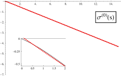
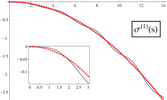
Figure 3. $\boldsymbol{\xi=0.6}$. The black curves are the solutions of the DEs (3.4) [left] and (3.17) [right] using a sequence of Taylor series of degree $12$. The dashed red curves are the asymptotic approximations (3.27) [left] and (3.29) [right]. The inset is the same plot zoomed-in on the origin.

The theory of [8], as reproduced in (2.4) above, predicts that this quantity is, to leading order in $1/\bar{\rho}$, itself of random matrix origin. As a test of its validity, Figure 2 displays a comparison of the empirical data and the theoretical predictions. Very good agreement is found for distances up to approximately one and a half times the average spacing between zeros, and furthermore the period of the oscillations are well matched for all distances in the display. On the other hand, as the distances increase, there is a systematic discrepancy at a quantitative level. Anticipation of the expanded form (2.4) not being in agreement for increasing distances comes when one graphically compares the corrections in (2.3) and (2.4) — recalling, in particular, that theoretically (2.3) and (2.4) agree to leading order. Thus one finds that their mismatch increases with increasing distance. On the other hand, the functional form from [11] used to obtain (2.3) can itself be numerically calculated. Its graphical form has for $\xi=1$ been compared against the two-point correlation of the same sequence of Riemann zeros as used here [6, Figures 12–17] or [7, Figures 3–7] and quantitative agreement is found for all distances displayed.

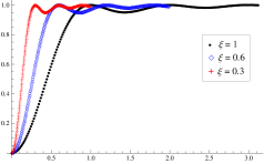
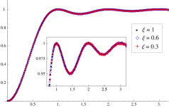
Figure 1. On the left is a plot of the raw 2-pt correlation function in the Riemann zero data, where each point has been deleted with probability $(1-\xi)$. The figure on the right contains the same data, which has been rescaled according to (2.8), showing the self-similarity property for varying $\xi$.

Figure 2. Comparison of the $1/\bar{\rho}^{2}$ term in (2.4) [solid curve] (with $s\to s/\xi$) against (2.9) [crosses] (again with $s\to s/\xi$).

3. Spacing distributions

3.1. Fredholm determinant formulae

Although the $k$-point correlations cannot be empirically computed from the data beyond the case $k=2$, certain functionals of the correlations can be so computed. A specific example is the $n$-th nearest neighbour spacing distribution $p(n;s)$, $n=0,1,2,\dots$. In terms of the correlations, and assuming a translationally invariant system with constant density $\rho$, we have in the case $n=0$,

$$p(0;s)=\frac{\rho_{(2)}(s,0)}{\rho}+\frac{1}{\rho}\sum_{j=1}^{\infty}{(-1)^{j}\over j!}\int_{0}^{s}dx_{1}\cdots\int_{0}^{s}dx_{j}\,\rho_{(j+2)}(s,0,x_{1},\dots,x_{j}),$$ (3.1)

and similar formulae for general $n$; see e.g. [27, §8.1 & §9.1].

The calculation of the functional form of the scaled limit of $p(0;s)$ for $N\times N$ unitary matrices $U(N)$ chosen with Haar measure, or equivalently bulk scaled GUE matrices, is a celebrated problem in random matrix theory. First note that a Fredholm determinant can be expanded as a series involving multiple integrals with integrands given as determinants of the integral kernel. With this expansion one can show from the form of the scaled $k$-point correlation functions (1.3) that

$$p(0;s)={d^{2}\over ds^{2}}\det(\mathbb{I}-\mathbb{K}_{s}),$$ (3.2)

where $\mathbb{K}_{s}$ is the integral operator supported on $(0,s)$ with kernel

$$K(x,y)={\sin\pi(x-y)\over\pi(x-y)},$$

noting that the constant density $\rho$ is unity. The required working can be found, for example, in [27, §9.1]. This Fredholm determinant formula is equivalent to the expression

$${d^{2}\over ds^{2}}\prod_{l=0}^{\infty}(1-\lambda_{l}(s)),$$

where $1>\lambda_{1}(s)>\lambda_{2}(s)>\cdots>0$ are the eigenvalues of $\mathbb{K}_{s}$. Such a result, for the bulk scaled limit of GOE matrices, was first obtained by Gaudin [33], who also provided a computational scheme by relating the eigenvalues $\{\lambda_{l}(s)\}$ to the eigenvalues of the second order differential operator having the prolate spheroidal functions as eigenfunctions (see e.g. [27, §9.6.1]). Only recently has it been shown that there are numerical schemes based directly on (3.2) that exhibit exponentially fast convergence to the limiting value [14, 15].

Nearly two decades after the work of Gaudin, the Kyoto school of Jimbo et al. [37] expressed (3.2) as the so-called $\tau$-function for a particular Painlevé V system. Explicitly, it was shown that

$$\det(\mathbb{I}-\xi\mathbb{K}_{s})=\exp\int_{0}^{\pi s}{\sigma^{(0)}(t;\xi)\over t}\,dt,$$ (3.3)

where $\sigma$ satisfies the differential equation

$$(t\sigma^{\prime\prime})^{2}+4(t\sigma^{\prime}-\sigma)(t\sigma^{\prime}-\sigma+(\sigma^{\prime})^{2})=0$$ (3.4)

with small $t$ boundary conditions

$$\sigma^{(0)}(t;\xi)=-{\xi\over\pi}t-{\xi^{2}\over\pi^{2}}t^{2}+{\rm O}(t^{3}).$$ (3.5)

Note that the parameter $\xi$ introduced in (3.3) only enters in the characterisation through the boundary condition. For background theory relating to the Painlevé equations as they occur in random matrix theory we refer to [27, Ch. 8].

Although (3.2) only requires the case $\xi=1$, the Fredholm expansion formula used to derive (3.2) generalises to read

$$\det(\mathbb{I}-\xi\mathbb{K}_{s})=\sum_{j=0}^{\infty}{(-\xi)^{j}\over j!}\int_{0}^{s}dx_{1}\cdots\int_{0}^{s}dx_{j}\,\rho_{(j)}(x_{1},\dots,x_{j}),$$ (3.6)

(cf. eq. (3.1)). In the case $\xi=1$, this formula, via the inclusion/exclusion principle, shows $\det(1-\mathbb{K}_{s})$ can be interpreted as the probability, $E(0;s)$, say, that there are no zeros in an interval of length $s$ of the original data set. Thus we have

$$E(0;s)=\det(\mathbb{I}-\mathbb{K}_{s}).$$ (3.7)

In the case of $0<\xi<1$, (2.7) together with the inclusion/exclusion principle shows (3.6) is equal to the probability that there are no zeros in an interval of length $s$ in the data set corresponding to a thinning of the original data set by deleting each zero with probability $(1-\xi)$ — this is the procedure alluded to in the Introduction. With $p(0;s;\xi)$ denoting the corresponding distribution of the nearest neighbour spacing, (3.2) generalises to

$$p(0;s;\xi)=\frac{1}{\xi}\frac{d^{2}}{ds^{2}}\det\left(\mathbb{I}-\xi\mathbb{K}_{s}\right),$$ (3.8)

where the the constant density $\rho=\xi$ in this decimated system. We remark that the notation $p((0,s);\xi)$ has been used in [27, §8.1] to denote the generating function for the conditioned spacing distributions $\{p(n;s)\}_{n=0,1,\dots}$, corresponding to the conditioned gap probabilities in the next paragraph. These quantities are related by

$$\frac{1}{\xi}\;p(0;s;\xi)=p((0,s);\xi).$$ (3.9)

As just mentioned, another interpretation shows itself via the formula (see e.g. [27, eq. (8.1) together with (9.15)])

$$E(m;s)={(-1)^{m}\over m!}{\partial^{m}\over\partial\xi^{m}}\det(\mathbb{I}-\xi\mathbb{K}_{s})\Big{|}_{\xi=1},$$ (3.10)

where $E(m;s)$ denotes the probability of an interval $s$ in the original data set containing exactly $m$ zeros. This is referred to as a (conditioned) gap probability. Note that (3.10) reduces to (3.7) in the case $m=0$.

Both the expressions (3.2) and (3.3) have analogues for the eigenvalues of $U(N)$ itself, rather than their scaled limit. Let $\mathbb{K}_{s}^{N}$ denote the integral operator supported on $(0,s)$ with kernel $K_{N}(x,y)$ as specified by (2.1). The analogue of (3.8) is then the structurally identical formula

$$p^{N}(0;s;\xi)=\frac{1}{\xi}{d^{2}\over ds^{2}}\det(\mathbb{I}-\xi\mathbb{K}_{s}^{N}).$$ (3.11)

Here $p^{N}(0;s;\xi)$ denotes the nearest neighbour spacing distribution for matrices from $U(N)$ chosen with Haar measure, with $s$ the difference in neighbouring angles. The $\tau$-function formula (3.3) generalises to [32, eq. (1.33)]

$$\det(\mathbb{I}-\xi\mathbb{K}_{s}^{N})=\exp\Big{(}-\int_{0}^{\pi s/N}U(\cot\phi;\xi)\,d\phi\Big{)},$$ (3.12)

where $U$ satisfies the $\tilde{\sigma}$PVI equation (see e.g. [27, eq. (8.21)])

$$u^{\prime}((1+s^{2})u^{\prime\prime})^{2}+4(u^{\prime}(u-su^{\prime})+iv_{1}v_{2}v_{3}v_{4})^{2}+4\prod_{k=1}^{4}(u^{\prime}+v_{k}^{2})=0,$$ (3.13)

with $u(s)=U(s;\xi)$ and parameters

$$v_{1}=v_{2}=v_{3}=0,\quad v_{4}=N,$$

subject to the boundary condition $u(s)\sim\xi N/\pi$ as $s\to\infty$.

3.2. Finite $N$ correction for the nearest neighbour spacing

Our interest is in the leading correction term to the large $N$ form of (3.11). Since, from (2.1),

$$K_{N}(x,y)={\sin\pi(x-y)\over\pi(x-y)}+{\pi(x-y)\over 6N^{2}}\sin\pi(x-y)+{\rm O}\Big{(}{1\over N^{4}}\Big{)},$$

we see that this correction term is of order $1/N^{2}$. Specifically

$$\det(\mathbb{I}-\xi\mathbb{K}_{s}^{N})=\det(\mathbb{I}-\xi\mathbb{K}_{s})\left[1-\frac{\xi}{N^{2}}{\rm Tr}\,\Big{(}(\mathbb{I}-\xi\mathbb{K}_{s})^{-1}L_{s}\Big{)}\right]+{\rm O}\Big{(}{1\over N^{4}}\Big{)},$$ (3.14)

where $L_{s}$ is the integral operator on $(0,s)$ with kernel $(\pi(x-y)/6)\sin\pi(x-y)$. We remark that with $R(x,y)$ denoting the resolvent kernel — that is the kernel supported on $(0,s)$ of the integral operator $\xi\mathbb{K}_{s}(\mathbb{I}-\xi\mathbb{K}_{s})^{-1}$ — straightforward manipulation shows

$${\rm Tr}\,\Big{(}(\mathbb{I}-\xi\mathbb{K}_{s})^{-1}L_{s}\Big{)}={\pi\over 6}\int_{0}^{s}dx\int_{0}^{s}dy\,R(x,y)(y-x)\sin\pi(y-x).$$

The expansion (3.14) tells us that in relation to the representation (3.12) we should change variables and write

$$-{1\over N}U(\cot X/N;\xi)={\sigma^{(0)}(X)\over X}+{1\over N^{2}}{\sigma^{(1)}(X)\over X}+{\rm O}\Big{(}{1\over N^{4}}\Big{)}.$$ (3.15)

This implies the expansion

$$\det(\mathbb{I}-\xi\mathbb{K}_{s}^{N})=\exp\left(\int_{0}^{\pi s}{\sigma^{(0)}(X)\over X}\,dX\right)\left(1+{1\over N^{2}}\int_{0}^{\pi s}{\sigma^{(1)}(X)\over X}\,dX+{\rm O}\Big{(}{1\over N^{4}}\Big{)}\right).$$ (3.16)

Both $\sigma^{(0)}$ and $\sigma^{(1)}$ also depend on $\xi$ (which, as mentioned below (3.5), enters through the boundary conditions), but for notational convenience this has been suppressed. As noted above, $\sigma^{(0)}$ satisfies the particular Painlevé V equation in sigma form (3.4) with boundary condition (3.5). By changing variables $s=\cot X/N$ in (3.13) and introducing the expansion (3.15), the equation (3.4) can be reproduced (a fact already known from [31]), and moreover a linear differential equation for $\sigma^{(1)}(X)$ with coefficients involving $\sigma^{(0)}(X)$, can be obtained.

Proposition 3.1.

With $\sigma^{(0)}(X)$, $\sigma^{(1)}(X)$ related to $U(s;\xi)$ in (3.12) by (3.15) we have that $\sigma^{(0)}(X)$ satisfies the particular Painlevé V equation in sigma form (3.4) with boundary condition (3.5), while $\sigma^{(1)}(X)$ satisfies the second order, linear differential equation

$$A(s)y^{\prime\prime}(s)+B(s)y^{\prime}(s)+C(s)y(s)=D(s),$$ (3.17)

where, with $\sigma(s)=\sigma^{(0)}(s)$,

$$A(s) =2s^{2}\sigma^{\prime\prime}(s),$$

$$B(s) =-8\sigma^{\prime}(s)\sigma(s)+12s(\sigma^{\prime}(s))^{2}+8s\Big{(}s\sigma^{\prime}(s)-\sigma(s)\Big{)},$$

$$C(s) =-4(\sigma^{\prime}(s))^{2}-8\Big{(}s\sigma^{\prime}(s)-\sigma(s)\Big{)},$$

$$D(s) =-\frac{4}{3}s^{2}\sigma^{\prime\prime}(s)\left(\sigma(s)-s\sigma^{\prime}(s)-{s^{2}\over 2}\sigma^{\prime\prime}(s)\right)$$

$$-\frac{4}{3}(s\sigma^{\prime}(s)-\sigma(s))\Big{(}3(\sigma(s))^{2}+2s\sigma(s)\big{(}s-\sigma^{\prime}(s)\big{)}-2s^{2}\sigma^{\prime}(s)\big{(}s+\sigma^{\prime}(s)\big{)}\Big{)}.$$

The corresponding $s\to 0^{+}$ boundary condition is

$$\sigma^{(1)}(s) =-\Big{(}s^{4}{\xi^{2}\over 9\pi^{2}}+s^{5}{5\xi^{3}\over 36\pi^{3}}+{\rm O}(s^{6})\Big{)}.$$ (3.18)

Proof.  We see there are three main terms in (3.13). Changing variables $s=\cot X/N$ and introducing the expansion (3.15) in the first gives

$$\Big{(}(1+s^{2})U^{\prime\prime}(s;\xi)\Big{)}^{2}=N^{2}\left\{X^{2}\left(\frac{d^{2}\sigma^{(0)}(X)}{dX^{2}}\right)^{2}\right\}$$

$$+4X^{2}\frac{d^{2}\sigma^{(0)}(X)}{dX^{2}}\left(\frac{1}{2}\frac{d^{2}\sigma^{(1)}(X)}{dX^{2}}-\frac{X}{3}\frac{d\sigma^{(0)}(X)}{dX}+\frac{\sigma^{(0)}(X)}{3}-\frac{X^{2}}{6}\frac{d^{2}\sigma^{(0)}(X)}{dX^{2}}\right),$$

up to terms of order $1/N^{4}$. Similarly expanding the other two main terms and then equating terms of order $N^{2}$ gives (3.4), while equating terms independent of $N$ gives (3.17).

In relation to the boundary conditions, for $U(s;\xi)$ in (3.12) we know from [27, eq. (8.78)], further extended to the next order, that for large $s$

$$U(s;\xi)= c+\frac{c^{2}}{s}+\frac{c^{3}}{s^{2}}+c^{2}\frac{9c^{2}-N^{2}-2}{9s^{3}}+c^{3}\frac{36c^{2}-5N^{2}-19}{36s^{4}}$$

$$+c^{2}\frac{46-375c^{2}+450c^{4}+N^{2}(40-75c^{2})+4N^{4}}{450s^{5}}+{\rm O}(s^{-6}),$$

where $c=\frac{\xi N}{\pi}$. Substituting in (3.15) and performing appropriate additional expansions we read off (3.18). $\square$

While we know of no other analytic formulae for the correction term to the spacing distribution for random matrix ensembles in the bulk, at an edge — specifically the soft edge — this task seems to have been first taken up by [20]. Aspects of this same problem at the hard edge are discussed in the recent works [25, 16, 48].

Let $f^{N}(x)[N^{-p}]$ denote the coefficient of $N^{-p}$ in the large $N$ expansion of $f^{N}(x)$. Then we have from (3.16) that

$$\det(\mathbb{I}-\xi\mathbb{K}_{s}^{N})[N^{-2}]=\Big{(}\int_{0}^{\pi s}{\sigma^{(1)}(X)\over X}\,dX\Big{)}\exp\Big{(}\int_{0}^{\pi s}{\sigma^{(0)}(X)\over X}\,dX\Big{)}.$$ (3.19)

One use of Proposition 3.1 is to be able to deduce the explicit form of the small and large distance expansions of (3.19). We will consider first the small $s$ expansion.

Corollary 3.2.

We have

$$\sigma^{(0)}(s)=-\frac{\xi s}{\pi}-\frac{\xi^{2}s^{2}}{\pi^{2}}-\frac{\xi^{3}s^{3}}{\pi^{3}}+\frac{1}{24}\left(\frac{8\xi^{2}}{3\pi^{2}}-\frac{24\xi^{4}}{\pi^{4}}\right)s^{4}+\left(\frac{5\xi^{3}}{36\pi^{3}}-\frac{\xi^{5}}{\pi^{5}}\right)s^{5}$$

$$+\left(-\frac{\xi^{6}}{\pi^{6}}+\frac{\xi^{4}}{6\pi^{4}}-\frac{2\xi^{2}}{225\pi^{2}}\right)s^{6}+\left(-\frac{\xi^{7}}{\pi^{7}}+\frac{7\xi^{5}}{36\pi^{5}}-\frac{7\xi^{3}}{675\pi^{3}}\right)s^{7}$$

$$+\left(-\frac{\xi^{8}}{\pi^{8}}+\frac{2\xi^{6}}{9\pi^{6}}-\frac{121\xi^{4}}{8100\pi^{4}}+\frac{\xi^{2}}{2205\pi^{2}}\right)s^{8}+\left(-\frac{\xi^{9}}{\pi^{9}}+\frac{\xi^{7}}{4\pi^{7}}-\frac{73\xi^{5}}{3600\pi^{5}}+\frac{761\xi^{3}}{1587600\pi^{3}}\right)s^{9}$$

$$+\mathrm{O}\left(s^{10}\right),$$ (3.20)

$$\sigma^{(1)}(s)=-{\xi^{2}s^{4}\over 9\pi^{2}}-{5\xi^{3}s^{5}\over 36\pi^{3}}+{(-15\xi^{4}+2\pi^{2}\xi^{2})s^{6}\over 90\pi^{4}}+{7(-15\xi^{5}+2\xi^{3}\pi^{2})s^{7}\over 540\pi^{5}}$$

$$-\frac{\left(1260\xi^{6}-203\pi^{2}\xi^{4}+12\pi^{4}\xi^{2}\right)s^{8}}{5670\pi^{6}}-\frac{\left(9450\xi^{7}-1785\pi^{2}\xi^{5}+83\pi^{4}\xi^{3}\right)s^{9}}{37800\pi^{7}}$$

$$+\mathrm{O}\left(s^{10}\right),$$ (3.21)

$$\det(\mathbb{I}-\xi\mathbb{K}^{N}_{s})[1] =1-\xi s+{\xi^{2}\pi^{2}\over 36}s^{4}-{\xi^{2}\pi^{4}\over 675}s^{6}+{\xi^{2}\pi^{6}\over 17640}s^{8}-\frac{\xi^{3}\pi^{6}}{291600}s^{9}+\mathrm{O}\left(s^{10}\right),$$ (3.22)

$$\det(\mathbb{I}-\xi\mathbb{K}_{s}^{N})[N^{-2}] =-{\xi^{2}\pi^{2}s^{4}\over 36}+{\xi^{2}\pi^{4}s^{6}\over 270}-{\xi^{2}\pi^{6}s^{8}\over 3780}+\frac{\xi^{3}\pi^{6}s^{9}}{48600}+\mathrm{O}\left(s^{10}\right),$$ (3.23)

$${2\pi\over N}p^{N}(0;2\pi s/N;\xi)[1] =\frac{\xi\pi^{2}s^{2}}{3}-\frac{2\xi\pi^{4}s^{4}}{45}+\frac{\xi\pi^{6}s^{6}}{315}-\frac{\xi^{2}\pi^{6}s^{7}}{4050}+\mathrm{O}\left(s^{8}\right),$$ (3.24)

$${2\pi\over N}p^{N}(0;2\pi s/N;\xi)[N^{-2}] =-\frac{\xi\pi^{2}s^{2}}{3}+\frac{\xi\pi^{4}s^{4}}{9}-\frac{2\xi\pi^{6}s^{6}}{135}+\frac{\xi^{2}\pi^{6}s^{7}}{675}+\mathrm{O}\left(s^{8}\right).$$ (3.25)

Proof.  The differential equation (3.4) admits a unique power series expansion about the origin with the first two terms given by (3.5). Expanding to higher order and solving for the unspecified coefficients gives (3.20). Substituting the expansion in (3.3) gives (3.22) for the small $s$ expansion of the Fredholm determinant; this series is also reported in [27, eq. (8.114)]. If we substitute (3.20) instead in the differential equation (3.17) and make use of the boundary condition (3.18) we find a unique power series expansion solution is generated which upon solving for the unspecified coefficients gives (3.21). Substituting (3.20) and (3.21) in the order $1/N^{2}$ correction term (3.19) gives (3.23). Recalling (3.11) and that we have a uniform density $\rho_{(1)}(s)=\xi$, we see (3.24) and (3.25) follow immediately from (3.22) and (3.23). $\square$

A consistency check can be placed on the above expansions. For this we note that it is also possible to use the characterisation (3.12) of $\det(\mathbb{I}-\xi\mathbb{K}_{s}^{N})$ to deduce the $N$-dependent small $s$ expansion [27, eq. (8.79)]

$$\det(\mathbb{I}-\xi\mathbb{K}_{s}^{N}) = 1-\xi s+{(1-1/N^{2})\xi^{2}\pi^{2}s^{4}\over 36}-{(1-1/N^{2})(2-3/N^{2})\over 1350}\xi^{2}\pi^{4}s^{6}$$ (3.26)

$$\!\!+{(1-1/N^{2})(1-2/N^{2})(3-5/N^{2})\over 52920}\xi^{2}\pi^{6}s^{8}+{\rm O}(s^{9}).$$

Expanding the RHS of (3.26) for large $N$ we obtain agreement with (3.22) for the leading form, and agreement with (3.23) for the next leading order $1/N^{2}$ term.

A noteworthy feature of (3.24) and (3.25) is the weak dependence on the dilution parameter $\xi$, which only changes from $\xi$ to $\xi^{2}$ at order $s^{7}$. One understanding of this result relates to the interpretation of (3.8), upon division by $\xi$, as the generating function for $\{p(n;s)\}_{n=0,1,\dots}$; recall (3.9). Then, in analogy with (3.10), $p(1;s)$ is obtained from (3.24) and (3.25) by applying $-{\partial\over\partial\xi}$ and setting $\xi=1$. It follows that $p(1;s)$ has leading small $s$ behaviour proportional to $s^{7}$, which is a known result [27, eq. (8.115)].

We turn our attention now to the behaviours for large $s$. The asymptotics of spacing distributions for random matrix ensembles in this regime have been reviewed in the recent work [28]. The case $\xi=1$ must be distinguished from $0<\xi<1$.

Corollary 3.3.

Suppose $0<\xi<1$. As $s\to\infty$ we have [43, eq. (1.16), with $\sigma_{0}(s/2)=\sigma^{(0)}(s)$ in our notation]

$$\sigma^{(0)}(s)=-ks+{1\over 2}k^{2}+{\rm O}\left({1\over s}\right),\qquad k=-\frac{1}{\pi}\log(1-\xi),$$ (3.27)

and thus

$$\det(\mathbb{I}-\xi\mathbb{K}_{s}^{N})[1]\mathop{\sim}\limits_{s\to\infty}A(\xi)s^{k^{2}/2}e^{-k\pi s}.$$ (3.28)

Also

$$\sigma^{(1)}(s)=-{k^{2}s^{2}\over 6}+{\rm O}(s)$$ (3.29)

and this together with (3.28) implies

$$\det(\mathbb{I}-\xi\mathbb{K}_{s}^{N})[N^{-2}]=A(\xi)s^{k^{2}/2}e^{-k\pi s}\left(-{k^{2}\over 12}(\pi s)^{2}+{\rm O}(s)\right).$$ (3.30)

Suppose instead $\xi=1$. In this case, for $s\to\infty$ we have

$$\sigma^{(0)}(s)=-\frac{s^{2}}{4}-\frac{1}{4}+{\rm O}\left({1\over s^{2}}\right),$$ (3.31)

which is equivalent to the expansion

$$\det(\mathbb{I}-\mathbb{K}_{s}^{N})[1]\mathop{\sim}\limits_{s\to\infty}A(1){e^{-(\pi s)^{2}/8}\over(\pi s)^{1/4}}.$$ (3.32)

We also have

$$\sigma^{(1)}(s)=-\frac{s^{4}}{48}+\frac{s^{2}}{48}+{\rm O}(1),$$ (3.33)

which when combined with (3.32) is equivalent to

$$\det(\mathbb{I}-\xi\mathbb{K}_{s}^{N})[N^{-2}]=A(1){e^{-(\pi s)^{2}/8}\over(\pi s)^{1/4}}\left(-{(\pi s)^{4}\over 192}+{(\pi s)^{2}\over 96}+{\rm O}(s)\right).$$ (3.34)

Thus, for large $s$

$${2\pi\over N}p^{N}(0;2\pi s/N;\xi)[1] \mathop{\sim}\limits_{s\to\infty}\left\{\begin{array}[]{lc}\frac{A(\xi)}{\xi}(k\pi)^{2}s^{k^{2}/2}e^{-k\pi s},&0<\xi<1,\\ A(1)\frac{\pi^{15/4}}{16}s^{7/4}e^{-(\pi s)^{2}/8},&\xi=1,\end{array}\right.$$ (3.37)

$${2\pi\over N}p^{N}(0;2\pi s/N;\xi)[N^{-2}] \mathop{\sim}\limits_{s\to\infty}\left\{\begin{array}[]{lc}-\frac{A(\xi)}{\xi}\frac{(k\pi)^{4}}{12}s^{k^{2}/2+2}e^{-k\pi s},&0<\xi<1,\\ -A(1)\frac{\pi^{31/4}}{3072}s^{23/4}e^{-(\pi s)^{2}/8},&\xi=1.\end{array}\right.$$ (3.40)

Proof.  As noted, the expansion (3.27) can be read off from [43], and this substituted in (3.3) gives (3.28). The value of $A(\xi)$ is given in [17, eq. (1.14)], although its derivation requires different methods [19, 2]. Substituting (3.27) in (3.17) and solving for large $s$ gives (3.29), and this together with knowledge of (3.28) gives (3.30).

From the definition of $k$, we see that the behaviour (3.27) breaks down when $\xi=1$. In that case we have, instead of (3.27), the large $s$ expansion (3.31). This follows from (3.3) and knowledge of the leading two terms of the large $s$ form of $\det(\mathbb{I}-\mathbb{K}_{s})$ [24, 54] as given by (3.32). Substituting (3.31) in (3.17) and solving for large $s$ gives (3.33). Then substituting this in (3.19) and using (3.32), we see that the large $s$ form of the $1/N^{2}$ correction term (3.19) for $\xi=1$ is given by (3.34).

To obtain the behaviour of the spacing distribution we use (3.28), (3.30), (3.32) and (3.34) in conjunction with (3.11) and so deduce (3.37) and (3.40). $\square$

Numerical methods to be discussed in Section 4 allow the large $s$ forms of $\sigma^{(0)}(s)$ and $\sigma^{(1)}(s)$ to be compared against their computed values from the differential equations; see Figures 5–4. A prominent feature seen upon differentiating the transcendents is that for $0<\xi<1$ higher order terms in the large $s$ expansion are oscillatory, as known from the analytic work of McCoy and Tang [43] in the case of $\sigma^{(0)}(s)$. Since there is no such effect for $\xi=1$, we display only the transcendent and its asymptotic form, and not the derivative. The asymptotic form in this case is functionally distinct from that for $0<\xi<1$ — note that the quantity $k$ in the latter actually diverges at $\xi=1$.

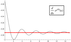
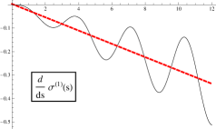
Figure 4. $\boldsymbol{\xi=0.6}$. These are the derivatives w.r.t. $s$ of the corresponding curves in Figure 3.

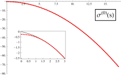
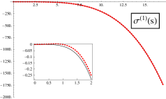
Figure 5. $\boldsymbol{\xi=1}$. The black curves are the solutions of the DEs (3.4) [left] and (3.17) [right] using a sequence of Taylor series of degree $35$. The dashed red curves are the asymptotic approximations (3.31) [left] and (3.33) [right]. The inset is the same plot zoomed-in on the origin.

A variation on the process of deleting each zero with the (constant) probability $1-\xi$ is to delete with probability $1-\xi(x)$, with $x=0$ corresponding to some pre-determined origin in the data. Since upon the scaling (1.1) the original data set is translationally invariant, an ensemble can be generated by varying the origin. The corresponding $k$-point correlation, $\rho_{(k)}(x_{1},\dots,x_{k};\xi(x))$ say, has the factorisation property

$$\rho_{(k)}(x_{1},\dots,x_{k};\xi(x))=\left(\prod_{l=1}^{k}\xi(x_{l})\right)\rho_{(k)}(x_{1},\dots,x_{k};1)$$

(cf. (2.7)). Thus in this circumstance the correlation kernel in (1.3) should be replaced by

$$\big{(}\xi(x_{j})\xi(x_{l})\big{)}^{1/2}\frac{\sin\pi(x_{j}-x_{l})}{\pi(x_{j}-x_{l})}.$$ (3.41)

Denoting the integral operator supported on $(0,s)$ with kernel (3.41) by $\mathbb{K}_{s}[\xi]$, the probability that an interval of size $s$ from the origin has no zeros is equal to $\det(1-\mathbb{K}_{s}[\xi])$. Subject to $\xi(x)$ having the functional form $\xi(x/s)=v(y)$, $y=x/s$ with $v(y)$ analytic on $[0,1]$, then (for large $s$) the expansion (3.28) generalises to [41, Theorem 2.1]

$$\det(1-\mathbb{K}_{s}[\xi])\sim C[\xi]s^{(a_{0}^{2}+a_{1}^{2})/4}e^{-\pi k_{v}s},$$

where

$$k_{v}=-\frac{1}{\pi}\int_{0}^{1}\log\big{(}1-v(x)\big{)}dx,\qquad a_{y}=-\frac{1}{\pi}\log\big{(}1-v(y)\big{)},$$

and for a certain explicit $C[\xi]$. Unfortunately the requirement that $\xi$ scale with $s$ prohibits probing this process in the Riemann zeros data. This is similarly true of the choice $\xi=1-e^{-2\kappa s}$ recently studied for large $s$ in [18].

3.3. Alternative characterisation of finite $N$ correction for nearest neighbour spacing

We see from (3.11) that to obtain the order $1/N^{2}$ correction to the limiting spacing distribution from knowledge of the $1/N^{2}$ correction to the gap probability, the second derivative with respect to $s$ of the latter must be taken. In fact, as first shown in [30] and further refined in [31], the second derivative can be incorporated within the Painlevé theory. Specifically, we have from [31] (again recalling (3.9)) that

$$p(0;s;\xi)={\xi\pi^{2}s^{2}\over 3}\exp\int_{0}^{2\pi s}u^{(0)}(t;\xi)\,{dt\over t},$$

where $u^{(0)}$ satisfies the particular, modified $\sigma$PV equation

$$\Big{(}su^{\prime\prime}(s)\Big{)}^{2}+\Big{(}su^{\prime}(s)-u(s)\Big{)}\Big{(}su^{\prime}(s)-u(s)-4+4(u^{\prime}(s))^{2}\Big{)}-16\Big{(}u^{\prime}(s)\Big{)}^{2}=0$$ (3.42)

subject to the small $s$ boundary condition

$$u^{(0)}(s;\xi)=-{1\over 15}s^{2}+{\rm O}(s^{4})-{\xi\over 8640\pi}\Big{(}s^{5}+{\rm O}(s^{7})\Big{)}.$$ (3.43)

Moreover, the result [31, eq. (5.16)] also tells us that for finite $N$

$${2\pi\over N}p^{N}(0;2\pi s/N;\xi)={\xi\over 3}(N^{2}-1)\sin^{2}{\pi s\over N}\exp\left(-\int_{0}^{\pi s/N}V(\cot\phi;\xi)\,d\phi\right),$$

where $V$ satisfies the $\tilde{\sigma}$PVI equation (3.13) with $u(s)=V(s;\xi)$ and parameters

$$v_{1}=v_{4}=0,\quad v_{2}=-N,\quad v_{3}=-2.$$ (3.44)

Analogous to (3.15), in keeping with the correction to the large $N$ form being of order $1/N^{2}$, we expand

$$-{1\over N}V(\cot X/(2N);\xi)={u^{(0)}(X)\over X}+{1\over N^{2}}{u^{(1)}(X)\over X}+{\rm O}\left({1\over N^{4}}\right),$$

so that

$${2\pi\over N}p^{N}(0;2\pi s/N;\xi) =\frac{\xi\pi^{2}s^{2}}{3}\exp\left(\int_{0}^{2\pi s}{u^{(0)}(X)\over X}\,dX\right)$$

$$\times\left(1-\frac{1}{N^{2}}-\frac{\pi^{2}s^{2}}{3N^{2}}+\frac{1}{N^{2}}\int_{0}^{2\pi s}{u^{(1)}(X)\over X}\,dX+{\rm O}\left({1\over N^{4}}\right)\right).$$ (3.45)

We know that $u^{(0)}(X)$ satisfies the nonlinear equation (3.42) subject to the boundary condition (3.43). Analogous to Proposition 3.1 it is possible to specify $u^{(1)}(X)$ as a second order linear differential equation with coefficients involving $u^{(0)}(X)$.

Proposition 3.4.

We have that $u^{(1)}(X)$ satisfies the second order, linear differential equation

$$\tilde{A}(s)y^{\prime\prime}(s)+\tilde{B}(s)y^{\prime}(s)+\tilde{C}(s)y(s)=\tilde{D}(s),$$ (3.46)

where, with $u(s)=u^{(0)}(s)$,

$$\tilde{A}(s) =8s^{2}u^{\prime\prime}(s),$$

$$\tilde{B}(s) =8\left(6s(u^{\prime}(s))^{2}+s^{2}u^{\prime}(s)-2s-su(s)-16u^{\prime}(s)-4u(s)u^{\prime}(s)\right),$$

$$\tilde{C}(s) =8\left(2+u(s)-su^{\prime}(s)-2(u^{\prime}(s))^{2}\right),$$

$$\tilde{D}(s) =\frac{2}{3}\Big{[}s^{2}u^{\prime\prime}(s)\Big{(}s^{2}u^{\prime\prime}(s)+2su^{\prime}(s)-2u(s)\Big{)}+s^{4}u^{\prime}(s)^{2}+4s^{3}u^{\prime}(s)^{3}$$

$$-2s^{3}u(s)u^{\prime}(s)-2s^{3}u^{\prime}(s)+16s^{2}u^{\prime}(s)^{2}+s^{2}u(s)^{2}+2s^{2}u(s)$$

$$-10su(s)^{2}u^{\prime}(s)-64su(s)u^{\prime}(s)-96su^{\prime}(s)+6u(s)^{3}+48u(s)^{2}+96u(s)\Big{]}.$$

The equation must be solved subject to the $s\to 0^{+}$ boundary condition

$$u^{(1)}(s) =\frac{4}{15}s^{2}-\frac{13}{6300}s^{4}+\frac{\xi}{1728\pi}s^{5}+{\rm O}(s^{6}).$$ (3.47)

Proof.  We apply the same technique as in Proposition 3.1 to the $\tilde{\sigma}$PVI equation (3.13) with parameters (3.44); that is we change variables $s=\cot X/(2N)$ and we find the terms of order $N^{2}$ give (3.42), while the terms of order $1$ give (3.46). For the boundary condition on $u^{(0)}(s)$, we have (3.43), which we extend to degree $6$ using (3.42). Then we combine this series with (3.46) to obtain the boundary condition on $u^{(1)}(s)$. $\square$

One check on the consistency of Proposition 3.4 is to verify that substitution of (3.47) and the first few terms of the power series solution of (3.42) into (3.45), reproduces the expansion (3.25). We find that this is indeed the case.

The required consistency between (3.45), and (3.16) combined with (3.11), together with knowledge of the large $s$ asymptotic forms in Corollary 3.3 give information on the large $s$ behaviour of $u^{(0)}(s)$ and $u^{(1)}(s)$. In relation to $u^{(0)}(s)$, for $0<\xi<1$, we have [43, eq. (1.26), with $\tilde{\sigma}_{2}(s/4)=u^{(0)}(s)$ in our notation]

$$u^{(0)}(s,\xi)=-\frac{ks}{2}+\frac{k^{2}}{2}-2+{\rm O}\left(\frac{1}{s}\right),$$ (3.48)

(up to a correction $b_{0}(n)\to-b_{0}(n)$ in [43, eq. (1.13)]) with $k$ as in (3.27). From [43] we know that the ${\rm O}(1/s)$ term in (3.48) is oscillatory. This is clearly displayed in Figure 6, where we compare a numerical solution of the differential equation (3.42), with [43, eq. (1.26)] as given in (3.48) with the oscillatory term O$(1/s)$ included. These oscillatory terms have concrete significance for the deduction of the functional form of $u^{(1)}(s,\xi)$ in the large $s$ limit, as if we are to substitute (3.48) for this purpose in the differential equation (3.46), we find a result inconsistent with (3.40). Consistency with the latter and (3.29) requires

$$u^{(1)}(s,\xi)=\frac{s^{2}}{6}+\mathrm{O}(s).$$ (3.49)

Note that this leading term is independent of $\xi$. From Figure 6 we also see that there are oscillatory sub-leading terms in (3.49); the graphs of the derivatives in Figure 7 indicate that these oscillations begin with the O$(s)$ term.

For $\xi=1$, we have consistency with (3.37) when

$$u^{(0)}(s,1)=-\frac{s^{2}}{16}-\frac{1}{4}+{\rm O}\left(\frac{1}{s}\right),$$ (3.50)

and substitution of this in (3.46) gives

$$u^{(1)}(s,1)=-\frac{s^{4}}{768}+\frac{43s^{2}}{192}+{\rm O}\left(1\right);$$ (3.51)

see Figure 8 for comparisons of these asymptotic forms against numerically generated solutions of the corresponding differential equations.

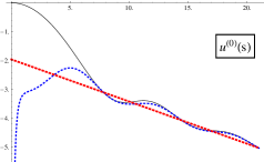
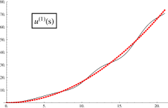
Figure 6. $\boldsymbol{\xi=0.6}$. The black curves are numerical solutions of the DEs (3.42) [left] and (3.46) [right] using a sequence of Taylor series of degree $12$. The dashed red curves are the asymptotic approximations (3.48) [left] and (3.49) [right]. The dashed blue curve in the graph on the left is a plot of the three leading terms in [43, eq. (1.26)] with $n=2,\theta=0,k=\frac{1}{2\pi}\log(1-\xi)$ therein.

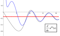
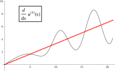
Figure 7. $\boldsymbol{\xi=0.6}$. These are the derivatives w.r.t. $s$ of the corresponding curves in Figure 6.

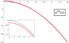
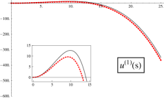
Figure 8. $\boldsymbol{\xi=1}$. The black curves are numerical solutions of the DEs (3.42) [left] and (3.46) [right] using a sequence of Taylor series of degree $35$. The dashed red curves are the asymptotic approximations (3.50) [left] and (3.51) [right]. The insets are the same plots zoomed-in on the origin.

4. Numerical power series solution of the differential equations and evaluation of the spacing distributions

The utility of Propositions 3.1 and 3.4 is that we can use a power series method together with computer packages to numerically compute to high accuracy the next-to-leading order term in the nearest neighbour spacing distribution (3.8); this can be done directly by computing the terms in (3.45) or via the second derivative of (3.19). Such power series methods were introduced as a technique to compute Painlevé transcendents associated with spacing distributions in random matrix theory in [49]. This was in relation to the soft edge. Subsequently the same numerical method was used for the computation of bulk spacings [27, §8.3.4]. The first point is to note that in generating a power series solution of the $\sigma$PV equation (3.4) about the origin, one finds a radius of convergence of approximately $8.5$ (for both $\xi=1$ and $\xi=0.6$). Inside the radius of convergence, this power series can be used to accurately evaluate the transcendent and its derivative, and from this data a new power series can be computed and the procedure iterated to cover the interval from $s=0$ to beyond $s=20$. With $\sigma^{(0)}(s)$ so determined, iterative power series solutions of the differential equation in Proposition 3.1 can be obtained. It is through this procedure, and its analogue starting with the differential equation (3.42) and proceeding to the differential equation of Proposition 3.4, that the graphs of $\sigma^{(0)}(s),\sigma^{(1)}(s),u^{(0)}(s),u^{(1)}(s)$ displayed in Figures 5–8 have been generated.

We remark that use of a power series method to generate solutions over a large interval seems necessary in the cases $0<\xi<1$. In particular, if in these cases one tries to use a computer algebra package to solve the differential equation (3.4) subject to initial conditions for $\sigma^{(0)}(x_{0})$ and $\sigma^{(0)}{}^{\prime}(x_{0})$ with $x_{0}$ small, as computed from the boundary condition (3.5) (with the latter further extended in accuracy as given in (3.20)), it is found that as $x$ is increased from $x_{0}$, the DE solver gives incorrect values, and furthermore soon diverges to a spurious pole.

Substitution of the piecewise functions for $\sigma^{(0)}(s)$ and $\sigma^{(1)}(s)$ into (3.16) gives us an approximation of $\det(\mathbb{I}-\xi\mathbb{K}_{s}^{N})$ up to the first order correction, and substitution into (3.19) isolates the correction term. Taking the second derivative with respect to $s$ we obtain Figures 9 and 10 respectively. Note that to obtain the comparison with the Riemann zero data in these figures, we have used the scalings (2.5) and (2.6) from [8]. Also in Figures 9 and 10 we plot an extrapolation of a sequence of finite calculations (3.11), similar to that in [8]: by calculating (3.11), with kernel (2.1), for 20 values of $N$ between 100 and 138 we extrapolate the limiting value of the nearest neighbour spacing and the next-to-leading order correction at each point. To graphical accuracy the extrapolated values are identical to those computed from the differential equation. Note that when $\xi=0.6$ the correction term shows more pronounced oscillations for finite $s$ values than its $\xi=1$ counterpart, a feature that seems to be be driven by oscillations in the functional forms for the corresponding Painlevé transcendents.

Figure 9. Comparison of Riemann zero nearest neighbour spacing (where each zero is scaled by the leading term in (1.1)) with the corresponding DE solution (ie. the second derivative of (3.16)). We also compare these to an extrapolated limit of a sequence of finite calculations as in (3.11).

Figure 10. Comparison of next-to-leading order corrections to the quantities in Figure 9.

Most strikingly, the predicted functional forms from random matrix theory show accurate agreement with the Riemann zero data both for $\xi=1$ [8], and upon thinning of the Riemann zero data set with $\xi=0.6$, for all displayed values of $s$. This is in contrast to what was found in Figure 2 for the two-point function, where the accuracy deteriorates after approximately one and a half units of the mean spacing. A significant difference between the two quantities that may explain this observation relates to the respective large $s$ forms. That is, the spacing distribution decays as an exponential or faster (see (3.45) with (3.48)–(3.51)), whereas the correction term for the two-point correlation function is an oscillatory order one quantity for all $s$ (see (2.2)). It follows that at a graphical level discrepancies in the case of the correction term to the spacing distribution functional formal form cannot be quantitatively probed in distinction to the situation with the correction term for the two-point correlation function.

In conclusion, our study corroborates the study of [8], and so lends further weight to the conjecture that correction terms to the Montgomery–Odlyzko law themselves have a random matrix interpretation. Specifically, as put forward in [8] as an extension of the earlier work [39], the results of our study are consistent with the hypothesis that the correction terms to the Montgomery–Odlyzko law for correlation functions and associated distribution functions of the Riemann zeros coincides with the ${\rm O}(1/N^{2})$ correction terms for the corresponding quantities of the eigenvalues of random unitary matrices. This holds with the relationship between $E$ and $N$ given by (2.5), and with the change of scale (2.6).

References

- [1] T.H. Baker and P.J. Forrester, Finite- fluctuation formulas for random matrices, J. Stat. Phys. 88 (1997), 1371–1386.
- [2] E. Basor, H. Widom, Toeplitz and Wiener-Hopf determinants with piecewise continuous symbols, Journal of Functional Analysis, 50 (1983), 387–413.
- [3] M.V. Berry, Riemann’s zeta function: a model for quantum chaos?, Quantum Chaos and Statistical Nuclear Physics (T.H. Seligman and H. Nishioka, eds.), Lecture Notes in Physics, 263, Springer, Berlin (1986), 1–17.
- [4] M.V. Berry and J.P. Keating, The Riemann zeros and eigenvalue asymptotics, SIAM Rev. 41 (1999), 236–266.
- [5] E. B. Bogomolny, Spectral statistics and periodic orbits, in New Directions in Quantum Chaos, Proceedings of the International School of Physics Enrico Fermi, course CXLIII, G. Casati, I. Guarneri, and U. Smilansky eds., Varenna (2000), 333–368.
- [6] E. Bogomolny, Quantum and arithmetical chaos, in Frontiers in Number Theory, Physics and Geometry: On Random Matrices, Zeta Functions and Dynamical Systems, Springer (2006), 3–106.
- [7] by same author, Riemann zeta function and quantum chaos, Prog. Th. Phys. Supp. 166 (2007), 19–36.
- [8] E. Bogomolny, O. Bohigas, P. Leboeuf, and A.C. Monastra, On the spacing distribution of the Riemann zeros: corrections to the asymptotic result, J. Phys. A 39 (2006), 10743–10754.
- [9] E.B. Bogomolny and J.P. Keating, Random matrix theory and the Riemann zeros I: three- and four-point correlations, Nonlinearity 8 (1995), 1115–1131.
- [10] by same author, Random matrix theory and the Riemann zeros II: -point correlations, Nonlinearity 9 (1996), 911–935.
- [11] by same author, Gutzwiller’s trace formula and spectral statistics: beyond the diagonal approximation, Phys. Rev. Lett. 77 (1996), 1472–1475.
- [12] O. Bohigas, Compound nucleus resonances, random matrices, quantum chaos, Recent perspectives in random matrix theory and number theory (F. Mezzadri and N.C. Snaith, eds.), London Mathematical Society Lecture Note Series 322, Cambridge University Press, Cambridge (2005), 147–183.
- [13] O. Bohigas and M.P. Pato, Missing levels in correlated spectra, Phys. Lett. B 595 (2004), 171–176.
- [14] F. Bornemann, On the numerical evaluation of Fredholm determinants, Math. Comp. 79 (2010), 871–915.
- [15] by same author, On the numerical evaluation of distributions in random matrix theory: a review, Markov Processes Relat. Fields 16 (2010), 803–866.
- [16] by same author, A note on the expansion of the smallest eigenvalue distribution at the hard edge, to appear Ann. Appl. Probab., arXiv:1504.00235
- [17] T. Bothner and A. Its, Asymptotics of a cubic sine kernel determinant, arXiv:1302.1871.
- [18] T. Bothner. P. Deift, A. Its and I. Krasovsky, On the asymptotic behaviour of a log gas in the bulk scaling limit in the presence of a varying external potential I, Commun. Math. Phys. 337 (2015), 1397–1463.
- [19] A. Budylin and V. Buslaev, Quasiclassical asymptotics of the resolvent of an integral convolution operator with a sine kernel on a finite interval, Algebra i Analiz, 7 (1995), 79–103.
- [20] L. Choup, Edgeworth expansion of the largest eigenvalue distribution function of GUE and LUE, Int. Math. Res. Notices 2006 doi:1155/IMRN/2006/61049 (2006).
- [21] B. Conrey, D. Farmer, J.P. Keating, M. Rubinstein and N. Snaith, Lower order terms in the full moment conjecture for the Riemann zeta function, J. Number Th. 128 (2008), 1516–1554.
- [22] J.B. Conrey and N.C. Snaith, In support on -correlation, Commun. Math. Phys. 330 (2014), 639–653.
- [23] M. Coram and P. Diaconis, New tests of the correspondence between unitary eigenvalues and the zeros of Riemann’s zeta function, J. Phys. A. 36 (2003), 2883–2906.
- [24] P.A. Deift, A.R. Its, and X. Zhou, A Riemann-Hilbert approach to asymptotic problems arising in the theory of random matrices and also in the theory of integrable statistical mechanics, Ann. Math. 146 (1997), 149–235.
- [25] A. Edelman, A. Guionnet, S.Péché, Beyond universality in random matrix theory, arXiv:1405.7590.
- [26] F.W.K. Firk and S.J. Miller, Nuclei, primes and the random matrix connection, Symmetry 1 (2009), 64–105.
- [27] P.J. Forrester, Log-gases and random matrices, Princeton University Press, Princeton, NJ, 2010.
- [28] by same author, Asymptotics of spacing distributions 50 years later, Random matrix theory, interacting particle systems and integrable systems, (ed. P. Deift and P. Forrester), MSRI Publications, 65 (2014), 199–222.
- [29] P.J. Forrester and A.M. Odlyzko, Gaussian unitary ensemble eigenvalues and Riemann function zeros: a non-linear equation for a new statistic, Phys. Rev. E 54 (1996), R4493–R4495.
- [30] P.J. Forrester and N.S. Witte, Exact Wigner surmise type evaluation of the spacing distribution in the bulk of the scaled random matrix ensembles, Lett. Math. Phys. 53 (2000), 195–200.
- [31] by same author, Application of the -function theory of Painlevé equations to random matrices: PVI, the JUE,CyUE, cJUE and scaled limits, Nagoya Math. J. 174 (2004), 29–114.
- [32] by same author, Random matrix theory and the sixth Painlevé equation, J.Phys. A 39 (2006), 12211–12233.
- [33] M. Gaudin, Sur la loi limite de l’espacement des valeurs propres d’une matrice aléatoire, Nucl. Phys. 25 (1961), 447–458.
- [34] F. Haake, Quantum signatures of chaos, 2nd ed., Springer, Berlin, 2000.
- [35] B. Hayes, The spectrum of Riemannium, American Scientist, 91 (2003), 296–300.
- [36] J. Illian, A. Penttinen, H. Stoyan and D. Stoyan, Statistical analysis and modelling of spatial point patterns, Wiley, 2008.
- [37] M. Jimbo, T. Miwa, Y. Môri, and M. Sato, Density matrix of an impenetrable Bose gas and the fifth Painlevé transcendent, Physica 1D (1980), 80–158.
- [38] N. M. Katz and P. Sarnak, Random matrices, Frobenius eigenvalues, and monodromy, Colloquium publications, 45, American Mathematical Society, Providence, RI, 1999.
- [39] J.P. Keating and N.C. Snaith, Random matrix theory and , Commun. Math. Phys. 214 (2001), 57–89.
- [40] by same author, Random matrices and -functions, J. Phys. A 36 (2003), 2859–2881.
- [41] N. Kitanine, K.K. Kozlowski, J.M. Maillet, N.A. Slavnov and V. Terras, Riemann–Hilbert approach to a generalised sine kernel and applications, Commun. Math. Phys. 291 (2009), 691–761.
- [42] T. Kriecherbauer and K. Schubert, Spacings — an example for universality in random matrix theory, Random matrices and iterated random function, Springer Proceedings in Mathematics and Statistics 53 (2013), 45–71.
- [43] B.M. McCoy and Sh. Tang, Connection formulae for Painlevé V functions: II. The -function Bose gas problem, Physica D 20 (1986), 187–216.
- [44] H.L. Montgomery, The pair correlation of zeros of the zeta function, Proc. Sympos. Pure Math., vol. 24, American Mathematical Society, Providence, RI (1973), 181–193.
- [45] H.L. Montgomery and K. Soundararajan, Beyond pair correlation, Paul Erdös and his mathematics. I, Bolyai Soc. Math. Stud. 11 (1999), 507–514.
- [46] A.M. Odlyzko, On the distribution of spacings between zeros of the zeta function, Math. Comput. 48 (1987), 273–308.
- [47] by same author, The -nd zero of the Riemann zeta function, Dynamical, Spectral, and Arithmeitc Zeta Functions (M. van Frankenhuysen and M.L. Lapidus, eds.), Contemporary Math. 2001, Amer. Math. Soc, Providence, RI, (2001), 139–144.
- [48] A. Perret and G. Schehr, Finite correction to the limiting distribution of the smallest eigenvalue of Wishart matrices, arXiv:1506.02387.
- [49] M. Prähofer and H. Spohn, Exact scaling functions for one-dimensional stationary KPZ growth, J. Stat. Phys. 108 (2004), 1071–1106.
- [50] B. Rodgers, The statistics of the zeros of the Riemann zeta-function and related topics, Ph.D. thesis, University of California at Los Angeles, 2013.
- [51] Z. Rudnick and P. Sarnak, Zeros of principal -functions and random matrix theory, Duke Math. J. (1995), 269–322.
- [52] K. Schubert, On the convergence of the nearest neighbour eigenvalue spacing distribution for orthogonal and symplectic ensembles, PhD thesis, Ruhr-Universität Bochum, Germany, 2012.
- [53] N.J.A. Sloane, The Online Encyclopedia of Integer Sequences, https://oeis.org/.
- [54] B. Valkó and B. Virág, Large gaps between random eigenvalues, Ann. Prob. 38, (2010), 1263–1279.
- [55] E.T. Whittaker and G.N. Watson, A course of modern analysis, 4th ed., Cambridge University Press, Cambridge, 1927.
- [56] Wikipedia, Hilbert–Pólya conjecture, http://en.wikipedia.org/wiki/Hilbert–Pólya_conjecture