Mass anomalous dimension of Adjoint QCD at large $N$ from twisted volume reduction

Abstract:

In this work we consider the $SU(N)$ gauge theory with two Dirac fermions in the adjoint representation, in the limit of large $N$. In this limit the infinite-volume physics of this model can be studied by means of the corresponding twisted reduced model defined on a single site lattice. Making use of this strategy we study the reduced model for various values of $N$ up to 289. By analyzing the eigenvalue distribution of the adjoint Dirac operator we test the conformality of the theory and extract the corresponding mass anomalous dimension.

1 Introduction

The $SU(2)$ gauge theory with two adjoint Dirac fermions, known as Minimal Walking Technicolor (MWT) [1, 2], has been the subject of many lattice studies, all of which have found it to be a conformal theory with a fairly small mass anomalous dimension $\gamma_{*}$ [3, 4, 5, 6, 7]. The most recent measurement obtained by fitting the mode number of the Dirac operator gave a very precise value [8]. The mode number method has also been used to follow the running of $\gamma$ over a range of energy scales for the $SU(3)$ theory with many light fundamental fermions [9].

The large $N$ version of MWT, the $SU(N)$ gauge theory with two adjoint fermions, is interesting for several reasons. From a phenomenological point of view, it is expected to be similar to the $SU(2)$ theory. For example, the universal first two perturbative coefficients of the beta function are independent of $N$. Hence, as in the case of MWT, they point towards the existence of an infrared fixed point with a mass anomalous dimension that is also independent of $N$. Moreover, numerical results for the mass anomalous dimension for the SU(2) and SU(3) theories appear to be in agreement [10], suggesting that this N–independence may be a good approximation all the way down to $N=2$. From a more theoretical point of view, the large $N$ theory is better suited for connecting with results obtained from different approaches, such as the AdS/CFT correspondence. Fortunately, the numerical study of the infinite volume theory at large $N$ is made possible by the concept of large $N$ volume independence. This implies the equivalence with a single site lattice reduced model, for which simulations can be performed at large values of $N$, that would be prohibitively expensive on a conventional $L^{4}$ lattice. In this context, the study of large $N$ Yang-Mills theory with adjoint fermions has attracted much attention  [11]- [20]. In this work we will be using the twisted reduction technique [21, 22]. For the adjoint fermion case the specific form of the action has been given in Ref. [23]. This model has been shown to lead to a softer $N$ dependence than the Adjoint Eguchi-Kawai model with periodic boundary conditions [12, 23]. The twisted model depends on the choice of the twist tensor. Here we will follow the same symmetric twist prescription as for the pure gauge theory, in which $N$ is taken as the square of an integer number $N=\hat{L}^{2}$, and the flux through each plane is equal to $\pm k\hat{L}$ (modulo $N$). With appropriate values of the integer $k$, this choice has proven effective in avoiding symmetry breaking for the pure gauge theory [24]. An important advantage of the twisted reduction method is that the dominant $1/N$ corrections amount to finite size effects on an $\hat{L}^{4}$ lattice. This allows an estimate of the values of $N$ at which the simulations should be performed. In this work we will be using values of $N$ up to 289, corresponding to lattices of size $17^{4}$.

In summary, the purpose of this paper is to analyze the behaviour of the $SU(N)$ gauge theory with two flavours of adjoint fermions in the large $N$ limit. Our main goal is to determine whether the theory has indeed a non-trivial infrared fixed point (IRFP) and to measure the mass anomalous dimension at this fixed point. In previous papers some of the present authors studied the behaviour of Wilson loops and the corresponding string tension [25, 26, 27, 28]. Although the results were consistent with the conformal behaviour characteristic of an IRFP, the extraction of the mass anomalous dimension had large uncertainties. Our methodology here will be based on an alternative procedure which has produced very precise estimates in the study of MWT [8]. Preliminary results have been presented in Refs. [29], [30].

The strategy is to determine the anomalous dimension from the structure of the eigenvalue density $\rho(\omega)$ of the massless Dirac operator $\not{D}$. The eigenvalue density is defined as

$$\rho(\omega)=\lim_{V\rightarrow\infty}\frac{1}{V}\sum_{k}\delta(w-w_{k})\quad,$$ (1)

where the sum runs over all eigenvalues $i\omega_{k}$ of $\not{D}$. In a mass–deformed conformal field theory (mCFT), this quantity should vanish for $w\rightarrow 0$ as [31]

$$\lim_{m\rightarrow 0}\lim_{V\rightarrow\infty}\rho(\omega)\propto\omega^{\frac{3-\gamma_{*}}{1+\gamma_{*}}},$$ (2)

where $\gamma_{*}$ is the mass anomalous dimension at the infrared fixed point, $V$ is the lattice volume, and $m$ is the mass. This behaviour should be contrasted with the one characteristic of a chirally broken theory where the eigenvalue density does not vanish at the origin.

In this paper we will use the previous idea to determine $\gamma_{*}$ for the large $N$ gauge theory with two adjoint quarks. It is clear from the previous formula that it is crucial to work in the region of very small masses and keeping finite volume effects under control. As a reference we will compare our result with those obtained for the pure gauge theory ($n_{f}=0$), for which the eigenvalue density has the characteristic behaviour of a chirally broken gauge theory.

The structure of the paper is as follows. In the next section we will collect all the technical aspects concerning the simulation and the extraction of the mass anomalous dimension from the data. In the following we will present the results of our analysis. The paper ends with the presentation of our conclusions.

2 Methodology

As explained in the introduction, our approach to the large $N$ limit is based on reduction. Hence, we simulate the twisted reduced $SU(N)$ model on a single site with two adjoint Dirac fermions [23]. In the large $N$ limit the theory is equivalent to the infinite volume lattice gauge theory. For finite $N=\hat{L}^{2}$, the corrections amount to finite volume corrections in an $\hat{L}^{4}$ lattice. Thus, it is important to keep track of the $N$-dependence which translates into the equivalent finite volume corrections. For that purpose we have performed simulations at values of $N$ ranging from 16 up to 289, the latter corresponding to an effective lattice volume of $17^{4}$. Our study has been done at two values of $b$, 0.35 and 0.36, and a large number of $\kappa$ values. The number of configurations used for the calculation of the eigenvalue spectrum at each value of $b$, $\kappa$ and $N$ are listed in Tab. 1. In addition we calculated the eigenvalue spectrum of the $n_{f}=0$ theory at $b=0.35,0.36$. For $N=121,289$, we used 10 configurations with $\kappa=0.170,0.175,0.180,0.185,0.190$, and for $N=841$, $b=0.36$ we used 4 configurations for $\kappa=0.190$.

		$N=16$	$N=25$	$N=49$	$N=121$	$N=289$
	$k$	1	2	3	3	5
	$\bar{k}/\sqrt{N}$	0.25	0.40	0.29	0.36	0.41
b	$\kappa$	$N=16$	$N=25$	$N=49$	$N=121$	$N=289$
0.36	0.160	20k	1200	500	20	20
	0.165	-	-	-	20	19
	0.170	-	-	-	20	15
0.35	0.160	-	-	-	40	20
	0.165	-	-	-	20	20
	0.170	-	-	-	20	13

Table 1: Number of configurations used for calculating the eigenvalue spectrum at each value of $b$, $\kappa$, $N$ and flux $k$. The integer parameter $\bar{k}$ satisfies $k\bar{k}=1$ (mod $\sqrt{N}$). All configurations are separated by at least 25 molecular dynamics updates, and at $N=289$ they are separated by 125 molecular dynamics updates.

As explained in the introduction, we have chosen the symmetric twist configuration, with values of the flux integer parameter $k$ given in Tab. 1. These fulfill the condition $k/\sqrt{N}>1/9$ which was found necessary for the pure gauge theory (TEK model) to respect the center symmetry [24]. This symmetry is a necessary ingredient in the proof of reduction by Eguchi and Kawai. The addition of light adjoint fermions should help in preserving the symmetry but, as shown in Ref. [23], adhering to the condition allows the study of the full range of $\kappa$ values and leads to a smoother $N$ dependence. As an example of the behaviour of Polyakov loops, which act as order parameters of the center symmetry, in Fig. 1 we display the expectation value of the modulus of the unit winding loop as a function of $N$. By definition, this quantity is always positive, but as seen in the figure its size decreases with $N$ for all values of $\kappa$.

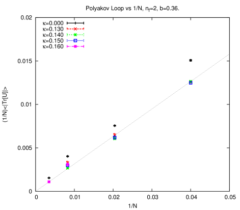
Figure 1: Polyakov loop: $\tfrac{1}{N}\left|\operatorname{Tr}U\right|$ vs $1/N$ for $n_{f}=2$. Must go to zero in the large $N$ limit for reduction to hold, which it does for all values of $\kappa$, where $\kappa=0$ corresponds to quenched $n_{f}=0$ data.

For each configuration we compute the low-lying spectrum of the modulus square of the massive lattice Wilson Dirac operator in the adjoint representation. This operator is positive definite and in the naive continuum limit corresponds to $a^{2}(-\not{D}^{2}+m^{2})$. Thus, its eigenvalues, labelled $(a\Omega)^{2}$, are related to those of $\not{D}$ by the expression

$$a\omega=\sqrt{(a\Omega)^{2}-m^{2}a^{2}}\quad,$$ (3)

where $a$ is the lattice spacing and $m$ is the adjoint quark mass. The lowest eigenvalue of our lattice operator defines the spectral gap. In the continuum it is bounded from below by $a^{2}m^{2}$. In the case of QCD and for the lattice Wilson Dirac operator, the median of the gap distribution was found empirically [32] to satisfy the relation

$$a\Omega_{0}\propto\frac{1}{2\kappa}-\frac{1}{2\kappa_{c}}.$$ (4)

so that $a\Omega_{0}$ is proportional to $am$. In our case, however, we expect that the bound is not saturated at finite $N$. The reason being the absence of zero-momentum quark states in the reduced model. Hence, quarks are then produced with at least the minimum momentum $2\pi/L$, whose square decreases linearly with $1/N$.

Since our main goal is the determination of the mass anomalous dimension with the idea presented in the introduction, it is important to study the region close to the critical point and for large values of $N$ to minimize small effective volume corrections. For that reason, our main analysis was based on the study of the lowest 2000 eigenvalues $(a\Omega)^{2}$ at $N=289$ and the lowest 1000 eigenvalues at $N=121$. The set of values of $b$ and $\kappa$ were given in Tab. 1. The computational cost increases considerably as we approach $\kappa_{c}$, explaining the smaller number of configurations for that case. Fortunately, the distribution of the lowest lying spectrum does not seem to fluctuate strongly at those values of $N$.

In determining the value of $\gamma_{*}$ from the distribution of eigenvalues there are certain alternative procedures which we will describe below.

2.1 Determination of the mass anomalous dimension $\gamma_{*}$

2.1.1 Determining $\gamma_{*}$ from a fit to the spectral density

In the continuum $\gamma_{*}$ could be determined by fitting the spectral density to the form expected for a mass-deformed conformal field theory, Eq. (2). However, in order to compare to the lattice data, it is more convenient to look at the spectral density of $-\not{D}^{2}$, given by:

$$\tilde{\rho}(\omega^{2})=\lim_{V\rightarrow\infty}\frac{1}{V}\sum_{k}\delta(w^{2}-w_{k}^{2})\propto(\omega^{2})^{\frac{1-\gamma_{*}}{1+\gamma_{*}}}.$$ (5)

This quantity is obtained on the lattice by counting the number of eigenvalues of the modulus square of the Wilson Dirac operator within a bin of size $\Delta^{2}$ around $(a\Omega)^{2}$. Representing this number by ${\cal N}(a\Omega,\Delta)$, the lattice spectral density is given by:

$$\tilde{\rho}_{L}((a\Omega)^{2})={1\over N^{2}\Delta^{2}}{\cal N}(a\Omega,\Delta),$$ (6)

where $N^{2}$ represents the lattice volume on the reduced lattice. The continuum formula for $\tilde{\rho}(\omega^{2})$ gives the following parameterisation for the lattice data:

$$\tilde{\rho}_{L}((a\Omega)^{2})=B\left[(a\Omega)^{2}-(am)^{2}\right]^{\frac{1-\gamma_{*}}{1+\gamma_{*}}},$$ (7)

allowing the determination of the three free parameters: $B$, $(am)^{2}$ and $\gamma_{*}$. The lowest part of the eigenvalue distribution is the one most affected by finite volume and finite mass effects, hence the fits have to be performed in an intermediate range of eigenvalues $a\Omega_{min}<a\Omega<a\Omega_{max}$, which preserves the separation of scales on the lattice,

$$\frac{1}{\sqrt{\mathrm{N}}}\ll am\ll a\Omega\ll 1.$$ (8)

From a practical viewpoint the 3-parameter fit demands very precise data in a wide range of eigenvalues and induces strong correlations between the parameters. In some cases the number of parameters can be reduced by assuming that the mass is negligibly small ($am=0$). Alternatively we can continue to work at finite mass but use information coming from the smallest eigenvalue to fix the parameter $(am)^{2}$ of the fit.

2.1.2 Determining $\gamma_{*}$ from a fit to the mode number

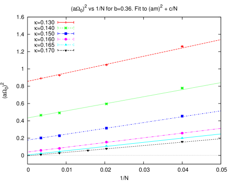
Figure 2: Median of the spectral gap of the modulus square of the Wilson Dirac operator, $({a\Omega}_{0})^{2}$, vs $1/N$. The fitting form $({a\Omega}_{0})^{2}=(am)^{2}+c/N$ fits all the data well.

Alternatively we can follow the procedure introduced in Ref. [8] and extract $\gamma_{*}$ from the mode number ${\nu}(\Omega)$ of the Dirac operator. It is simply defined as the number of eigenvalues of $(-\not{D}^{2}+m^{2})$ below some value $\Omega^{2}$. Hence, it is given by $V$ times the integral of the eigenvalue density. We can split this integral into two parts as follows

$${\nu}(\Omega)=2V\int_{0}^{\sqrt{\Omega_{IR}^{2}-m^{2}}}\rho(\omega)\,\,d\omega+2V\int_{\sqrt{\Omega_{IR}^{2}-m^{2}}}^{\sqrt{\Omega^{2}-m^{2}}}\rho(\omega)\,\,d\omega,$$ (9)

The first part contains the range of eigenvalues which are more sensitive to finite volume and/or finite mass effects. For the second part we can insert Eq. (2) and perform the integration to give

$${\nu}(\Omega)\simeq\nu(\Omega_{IR})-{\cal A}\left[\Omega^{2}_{IR}-m^{2}\right]^{\frac{2}{1+\gamma_{*}}}+{\cal A}\left[\Omega^{2}-m^{2}\right]^{\frac{2}{1+\gamma_{*}}}.$$ (10)

To determine ${\nu}(\Omega)$ on the lattice we just simply count the number of eigenvalues of the modulus square of the lattice Wilson massive Dirac operator below some value $(a\Omega)^{2}$. The continuum formula for the mode number implies that the lattice data can be parametrized as follows:

$$\nu_{L}(a\Omega)\simeq\nu_{0}+A\left[(a\Omega)^{2}-(am)^{2}\right]^{\frac{2}{1+\gamma_{*}}},$$ (11)

where

$$\nu_{0}=\nu_{L}(a\Omega_{IR})-A\left[(a\Omega_{IR})^{2}-(am)^{2}\right]^{\frac{2}{1+\gamma_{*}}}.$$ (12)

Eq. (11), normalised dividing by the lattice volume, is the expression used in Ref. [8] to fit the lattice data. This allows the determination of its four free parameters ($\nu_{0}$, $A$, $(am)^{2}$ and $\gamma_{*}$).

For the same reason as discussed before for the spectral density, one can attempt to reduce the number of parameters in the fit. If we assume that finite volume (i.e. finite $N$) effects are negligible we might take $\Omega_{IR}$ close to threshold making $\nu_{0}$ negligibly small compared to the other term. This leads to a simplified expression

$$\nu_{L}(a\Omega)\simeq A\left[(a\Omega)^{2}-(am)^{2}\right]^{\frac{2}{1+\gamma_{*}}}.$$ (13)

which can be used to fit its three parameters ($A,am,\gamma_{*}$) to the modenumber data in a range of eigenvalues $\Omega\in[\Omega_{min},\Omega_{max}]$ satisfying:

$$\frac{1}{\sqrt{\mathrm{N}}}\ll am\ll a\Omega_{IR}<a\Omega<a\Omega_{UV}\ll 1.$$ (14)

If we set $am=0$ in Eq. (13) we can reduce the number of free parameters even further. This is for example the strategy adopted in Ref. [9] where a 2–parameter fit to the mode number is used,

$$\nu_{L}(\Omega)\simeq A[(a\Omega)^{2}]^{\frac{2}{1+\gamma_{*}}}.$$ (15)

The sensitivity to the fit function, the volume, the mass parameter, or the fitting range will be used to estimate the systematic error in the determination of the mass anomalous dimension.

$b$	$\kappa$	$N=121$	$N=289$	$N=\infty$
0.36	0.160	0.0803(6)	0.0585(3)	0.0429(7)
	0.165	0.0433(4)	0.0224(2)	0.0074(5)
	0.170	0.0279(4)	0.0096(2)	-0.0036(4)
0.35	0.160	0.0997(9)	0.0815(4)	0.0683(9)
	0.165	0.0530(5)	0.0346(2)	0.0214(6)
	0.170	0.0281(4)	0.0105(4)	-0.0021(7)

Table 2: Lowest eigenvalues squared for each $b$, $\kappa$ and $N$, along with the extrapolation to $N=\infty$ which corresponds to the mass parameter $(am)^{2}$.

3 Results

3.1 Analysis of the two flavor case

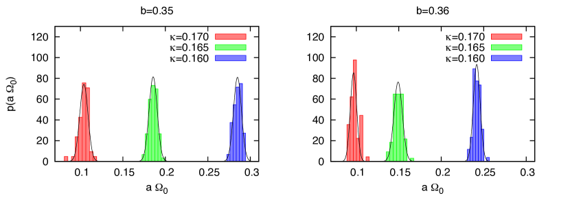
Figure 3: Probability distribution of the spectral gap of the Wilson Dirac operator for $N=289$ and various values of $\kappa$. The lines are fits to a gaussian distribution, Eq. (16).

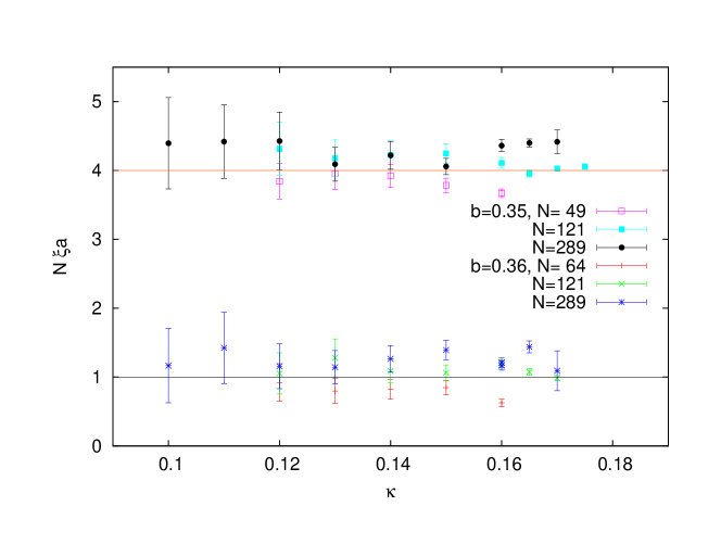
Figure 4: We display $N\xi a$ for our ensemble of $n_{f}=2$ configurations for $b=0.36$ and $b=0.35$ (displaced by 3 vertically for clarity), where $\xi a$ is the width of the probability distribution of the spectral gap of the Wilson Dirac operator.

In this section we will present the results of our study. Our first step is the analysis of the spectral gap of the hermitian Wilson–Dirac operator. To study how this quantity behaves as a function of $N$ and $\kappa$, we measure the lowest eigenvalue at $b=0.36$ on a range of configurations for $N=25-289$ and $\kappa=0.130-0.170$. As argued in the previous section, in the twisted model we expect the median of the gap distribution $({a\Omega}_{0})^{2}$ to differ from $(am)^{2}$ by a finite volume correction which, interpreted as non-zero momentum contribution, should depend linearly on $1/N$. Indeed, a linear fit of this kind seems to describe our non–perturbative data quite well, as shown in Fig. 2. This allows us to determine the mass parameter $(am)^{2}$ in the large $N$ limit, listed in Tab. 2.

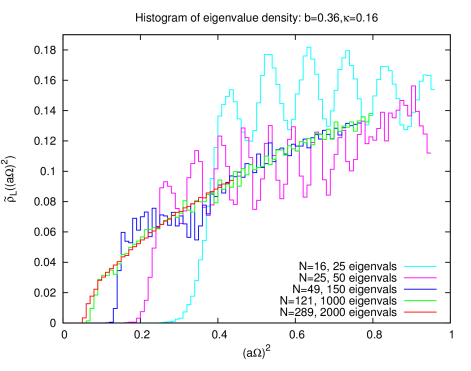
Figure 5: Spectral density $\tilde{\rho}_{L}((a\Omega)^{2})$ for $b=0.36$, $\kappa=0.160$, with a bin–size $\Delta^{2}=0.01$. There is agreement at all eigenvalues (except the very lowest couple of bins) between $N=121$ and $N=289$. For $N=49$ there is a qualitative difference for the lower eigenvalues, but the large ones are also in agreement.

We have analysed the probability distribution of the spectral gap $p({a\Omega}_{0})$ of the Wilson Dirac operator. In the large volume limit of QCD, the analysis in Ref. [32] showed that the distribution is gaussian:

$$p({a\Omega}_{0})\propto\exp\Big{\{}-{1\over 2(\xi a)^{2}}\left(a\Omega_{0}-\left\langle{a\Omega}_{0}\right\rangle\right)^{2}\Big{\}}\,$$ (16)

with median proportional to the bare current quark mass and width scaling with the volume and the lattice spacing approximately as $\xi a=a^{2}/\sqrt{V}$. In the reduced lattice this would imply $\xi a=1/N$. Fig. 3 shows $p({a\Omega}_{0})$ for $N=289$ at $b=0.35$ and $0.36$ and several values of $\kappa$. A gaussian fit describes the data well. The fitted distribution widths multiplied by $N$ are displayed in Fig. 4 for our $n_{f}=2$ configurations at several values of $N$ and $\kappa$. Our results follow rather well the behaviour also reported in QCD.

Let us now move on to describe our results for the distribution of eigenvalues. One of the main points is to analyze the $N$-dependence of this distribution. We already saw that this dependence affects the gap of the spectrum, but we expect this effect to have a small impact for higher eigenvalues. This can be seen in Fig. 5, which shows a histogram of the number of eigenvalues as a function of $(a\Omega)^{2}$, for $b=0.36$, $\kappa=0.160$. Comparing different values of $N$, we see agreement between $N=289$ and $N=121$ in all but the first two bins. For $N=49$, for $(a\Omega)^{2}\lesssim 0.4$ the behaviour is qualitatively different, but for higher eigenvalues we again see agreement with larger values of $N$. For $N=25$ and $N=16$ there are strong oscillations in the distributions, which are presumably the sum of the distributions of individual eigenvalues with the allowed discrete momenta.

figureEigenvalue density distribution at $b=0.35$ (left) and $b=0.36$ (right) for $\kappa=0.165,0.17$ and $N=121,289$.

We have seen that, at least for the two biggest values of $N$, the eigenvalue distribution roughly coincides beyond a certain threshold value. The question now is to see if this distribution behaves as expected from the IRFP hypothesis and to extract $\gamma_{*}$ from it. In the previous section we gave two alternative methods of fitting the data. One is to compare the eigenvalue distribution with Eq. (7). The other is to compute the mode number and fit it to Eq. (10) or to its simplified expression Eq. (13).

In performing a fit one has to select the range of values ${\Omega}_{\mathrm{min}}<\Omega<{\Omega}_{\mathrm{max}}$ to be fitted. A lower value of ${\Omega}_{\mathrm{min}}$ increases the sensitivity to the value of the mass $(am)^{2}$ but also risks to be more affected by finite effective volume (finite $N$) corrections. For the mode number fit the same is expected to happen for the parameter $\nu_{0}$. Furthermore, the narrower the fitting range the stronger the correlations among parameters leading to high uncertainties in $\gamma_{*}$.

If we use only the data which is least affected by finite volume and finite mass effects, we can produce our most precise determination of $\gamma_{*}$: Hence, we take our data of $N=289$ and $\kappa=0.17$ and fit the distribution of eigenvalues to Eq. (7) with $(am)^{2}$ set to zero. The upper edge of the fitting range $(a\Omega_{\mathrm{max}})^{2}$ covers almost all of the $N=289$ data. For the lower edge $(a\Omega_{\mathrm{min}})^{2}$ the cut is set to twice the lowest eigenvalue for $N=121$. The result for $b=0.36$ is $\gamma_{*}=0.268(2)$ and for $b=0.35$ is $\gamma_{*}=0.271(1)$. It is remarkable that both values of $b$ give consistent results within the purely statistical 1% errors. To give an idea of the quality of the fit we display the data in Fig. 3.1 together with the best fit. In the figure we also include the data of $N=121$ at both values of $b$. The fitted function also describes well the behaviour of the data at $N=121$, except for the smallest eigenvalues where finite volume effects should be mostly felt. The continuous line going through the $\kappa=0.165$ data was obtained fitting the corresponding data with $\gamma_{*}$ fixed to the value obtained at $\kappa=0.17$ and the mass square $(am)^{2}$ to the large $N$ extrapolated value given in Tab. 2.

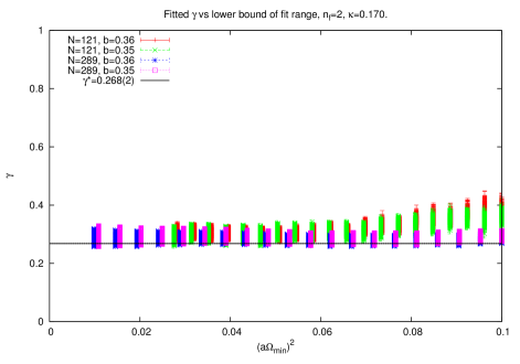
Figure 6: Fitted $\gamma_{*}$ as a function of $(a\Omega_{\rm min})^{2}$ from fitting the spectral density data to Eq. (7). For each point, a range of masses $(am)^{2}$ between zero and the lowest eigenvalue at $N=289$ are used, and the upper fit range bound $(a\Omega_{\rm max})^{2}$ is also varied over a range of values from 0.25 up to the largest value for which we have data. The black line shows our best estimate for $\gamma_{*}$ with statistical error only.

The analysis of the previous figure and fits indicates that our data look consistent with the predictions of an infrared fixed point with mass anomalous dimension close to $0.27$. In order to substantiate the claim of conformality, it is important to check the systematic uncertainties involved in our analysis and to compare our results with those corresponding to theories which are not conformal in the IR. The latter will be done in the next section where we will compare our $n_{f}=2$ results with those obtained for $n_{f}=0$. What we will now present is an evaluation of the systematic errors. This point will be analysed by estimating the effect of finite $N$ corrections, finite mass corrections and sensitivity to the fitting range. We will also test what results come out if we use the mode number instead of the eigenvalue density.

A good summary of the effect of all systematics on the value of $\gamma_{*}$ is provided by Fig. 6. Here we display different determinations of $\gamma_{*}$ for the $N=289$ and $N=121$ data by varying $\Omega_{\max}$, $\Omega_{\min}$ and $(am)^{2}$. The latter is varied within the range extending from zero to the minimum $N=289$ eigenvalue. The data is displayed as a function of $(a\Omega_{\min})^{2}$. For a large range of x-axis values all determinations of $\gamma_{*}$ (obtained by using different values of $\Omega_{\max}$ and $(am)^{2}$) fall within a horizontal strip whose width serves as an upper bound to our systematic error $\delta\gamma_{*}=0.05$. For larger values of $(a\Omega_{\min})^{2}$ the fitting range narrows, obviously leading to a wider spread of values of $\gamma_{*}$.

To better analyze the dependence of the fitted value of $\gamma_{*}$ with the remaining parameters, we display in Fig. 7 its correlation with the mass parameter used in the fits for all values $(a\Omega_{\max})^{2}$ and $(a\Omega_{\min})^{2}<0.07$. This shows that the main source of systematic errors is indeed the value of the mass.

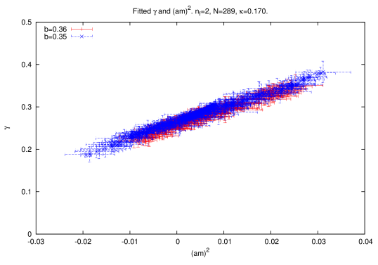
Figure 7: Fitted values of $(am)^{2}$ and $\gamma_{*}$ when both are taken as free parameters when fitting the spectral density data to Eq. (7), using $N=289$ configurations. There is a clear correlation between the two parameters.

figureFits to the mode number at $b=0.35$ (left) and $b=0.36$ (right) for $\kappa=0.165,0.17$ and $N=121,289$.

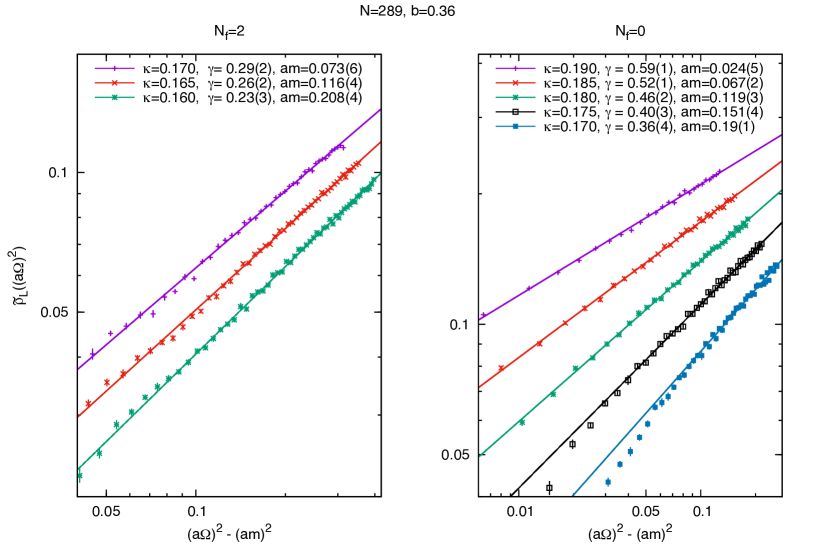
Figure 8: Eigenvalue density distribution, in log-log scale, at $b=0.36$ for $n_{f}=2$ and $n_{f}=0$. The lines correspond to the fits to Eq. ( 7) described in the text.

A similar analysis can be done for the mode number. Results are essentially compatible. In this case, one has an issue about which fitting formula one should use. Although the 4-parameter formula Eq. (10) should apply in all regions, there are strong correlations between the fitted parameters, so that for example a large range of values of $\gamma_{*}$ can produce a good fit by a suitable choice of the other 3 fit parameters. The more restrictive fitting formulas better constrain the fitted quantities, but have a limited range of applicability. For example Fig. 3.1 shows a fit to Eq. (13) using the same configurations and fit ranges as for the eigenvalue density in Fig. 3.1, which gives $\gamma_{*}=0.270(2)$ for $b=0.36$ and $\gamma_{*}=0.272(1)$ for $b=0.35$, which are in good agreement with the numbers determined from the eigenvalue density.

3.2 Comparison between zero and two flavors

The comparison between our $n_{f}=2$ results with those obtained for $n_{f}=0$ is essential to substantiate the claim of conformality. The latter theory is not conformal and should display a different behaviour. Indeed, for the pure Yang-Mills theory it makes no sense to speak of $\gamma_{*}$ itself, since there is no infrared fixed point. However, it still makes sense to study the behaviour of the spectral density and mode number distribution as a function of its argument.

To carry on the previous study, we generated pure gauge configurations at the same values of $b$ and $N$ and a range of $\kappa$ values, and repeated our previous analysis for this data. The $\kappa$ values were chosen in such a way as to explore similar small values of the minimum eigenvalue.

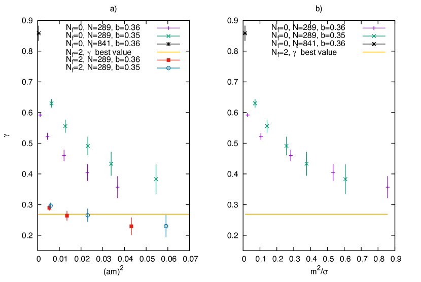
Figure 9: a) Dependence of the extracted value of $\gamma_{*}$ with the mass $(am)^{2}$ for $n_{f}\!=0\!$ and $n_{f}\!=\!2$. b) Dependence of the extracted value of $\gamma_{*}$ with $(m)^{2}/\sigma$ for $n_{f}\!=0\!$.

The fits to the spectral density for the largest values of $\kappa$ were qualitatively as good as those of $n_{f}=2$. Fig. 8 shows, in log-log scale, the fits to the lattice spectral densities for $n_{f}=2$ and $n_{f}=0$ at $b=0.36$. The values of $\gamma_{*}$ in this plot are obtained by fitting the spectral densities to Eq. ( 7). The mass $(am)^{2}$ is varied in the range $0.5(a\Omega_{0})^{2}\leq(am)^{2}\leq(a\Omega_{0})^{2}$, the number of bins is varied from 40 to 80, and the lower edge of the fit range is varied in the range $1.5(a\Omega_{0})^{2}\leq a\Omega_{\rm min}\leq 2(a\Omega_{0})^{2}$. The final point is an average over all of these choices for many bootstrap replicas of the data. Keeping $\gamma_{*}$ fixed to this average, the fits are repeated for each set of data in order to determine $am$. For this final fit the lower edge of the fit range is set to $2(a\Omega_{0})^{2}$. In all cases the $\chi^{2}$ per degree of freedom of the fit is below 2. Hence, from the quality of the fit to the spectral density one cannot deduce the presence of an infrared fixed point.

One remarkable difference appears when looking at the dependence of the extracted value of $\gamma_{*}$ with the mass $(am)^{2}$. The result is shown in Fig. 9a. The value of $\gamma_{*}$ seems quite stable for the $n_{f}=2$ case. This is what one expects in the vicinity of an infrared fixed point as the anomalous dimensions tends to a constant at the fixed point. The result for $n_{f}=0$ is quite different, showing a pronounced drop as we move away from the critical value of $\kappa$. For the smallest masses the fitted value of $\gamma_{*}$ reaches as high values as $0.8$. Notice that a value equal to $3$ would imply a constant value of the spectral density at the origin. Our data show a growing $\gamma_{*}$ for lighter masses but do not yet reach the value of 3 predicted by chiral symmetry breaking, through the Banks-Casher formula. This is probably due to finite volume and/or finite mass effects.

Another marked difference between the two cases appears in the dependence of the spectral densities on the bare inverse coupling $b$. In the conformal case one expects the coupling to be a marginally irrelevant operator close to the IRFP, in contrast to the $n_{f}=0$ case where it is marginally relevant and determines the lattice spacing. The values of $\gamma_{*}$ displayed in Fig. 9a for $n_{f}=2$ do indeed have a very small dependence on $b$. However, this dependence is large for the case of $n_{f}=0$. In the quenched case, the results corresponding to the two different couplings only show scaling when expressed in physical units in terms of the string tension. This is shown in Fig. 9b, where we have used the data for the $n_{f}=0$ string tension obtained in Refs. [33] ($\sigma a^{2}=0.09$ and $\sigma a^{2}=0.043$ for $b=0.35$ and $b=0.36$ respectively).

4 Conclusions

We have performed a measurement of the mass anomalous dimension $\gamma_{*}$ of the SU($N$) gauge theory with two adjoint Dirac fermions, in the large $N$ limit using the concept of large $N$ twisted reduction. Results from a single site lattice model at large values of $N$, have the expected qualitative behaviour of the spectral density and mode number of the adjoint massless Dirac operator. The distribution for small masses (extracted from the lowest eigenvalue) can be well-fitted with the expectations of an IRFP. From the data we extract a value of $\gamma_{*}=0.269\pm 0.002\pm 0.05$, where the first error is statistical and the second one systematic. This value is similar to previous lattice determinations of this quantity for the SU(2) theory.

Does our result provide conclusive evidence of the presence of an infrared fixed point for the SU($\infty$) gauge theory with 2 flavours of adjoint fermions? To try to answer this question we repeated the analysis for the $n_{f}=0$ case, which is known to have a completely different behaviour at criticality. However, we observe that the spectral densities at fixed $b$ and small quark mass, can also be fitted with the same formulas with a larger value of $\gamma_{*}$. This conveys a word of warning about drawing conclusions about the existence of an IRFP only from the capacity to fit the spectral density or mode number with a powerlike distribution. Nevertheless, there are marked differences between the behaviour observed in the $n_{f}=0$ and $n_{f}=2$ cases. One of them is the dependence of the result on the bare coupling $b$. The $n_{f}=2$ results for our two values of $b$, 0.35 and 0.36, are consistent with each other. This is not the case for the $n_{f}=0$ data. Although insensitivity to the bare coupling $b$ is certainly the expected result for an IRFP, it is difficult to exclude the fact that this is not simply due to the smaller value of the beta function when adding fermions in the adjoint. The second difference refers to the change of behaviour as we approach criticality $\kappa\longrightarrow\kappa_{c}$. The extracted value of $\gamma_{*}$ for $n_{f}=2$ remains fairly stable as one expects if the behaviour is indeed dictated by the presence of an IRFP. On the contrary for the $n_{f}=0$ data we observe a pronounced rise of the value of $\gamma_{*}$ as we approach criticality.

To improve on these results using this method, smaller fermion masses and larger volumes (i.e. larger values of $N$) would be required. Since finite volume effects are the dominant limitation, one possibility for future work would be to extend the single site lattice to a $2^{4}$ lattice.

References

- [1] F. Sannino and K. Tuominen, “Orientifold theory dynamics and symmetry breaking,” Phys. Rev. D 71, 051901 (2005) [arXiv:hep-ph/0405209].
- [2] M. A. Luty and T. Okui, “Conformal technicolor,” JHEP 0609, 070 (2006) [arXiv:hep-ph/0409274].
- [3] F. Bursa, L. Del Debbio, L. Keegan, C. Pica and T. Pickup, “Mass anomalous dimension in SU(2) with two adjoint fermions,” Phys. Rev. D 81, 014505 (2010) [arXiv:0910.4535 [hep-ph]].
- [4] L. Del Debbio, B. Lucini, A. Patella, C. Pica and A. Rago, “The infrared dynamics of Minimal Walking Technicolor,” Phys. Rev. D 82, 014510 (2010) [arXiv:1004.3206 [hep-lat]].
- [5] T. DeGrand, Y. Shamir and B. Svetitsky, “Infrared fixed point in SU(2) gauge theory with adjoint fermions,” Phys. Rev. D 83, 074507 (2011) [arXiv:1102.2843 [hep-lat]].
- [6] S. Catterall, L. Del Debbio, J. Giedt and L. Keegan, “MCRG Minimal Walking Technicolor,” Phys. Rev. D 85, 094501 (2012) [arXiv:1108.3794 [hep-ph]].
- [7] E. Bennett and B. Lucini, Eur. Phys. J. C 73 (2013) 2426 [arXiv:1209.5579 [hep-lat]].
- [8] A. Patella, “A precise determination of the psibar-psi anomalous dimension in conformal gauge theories,” Phys. Rev. D 86, 025006 (2012) [arXiv:1204.4432 [hep-lat]].
- [9] A. Cheng, A. Hasenfratz, G. Petropoulos and D. Schaich, “Scale-dependent mass anomalous dimension from Dirac eigenmodes,” JHEP 1307 (2013) 061 [arXiv:1301.1355 [hep-lat]].
- [10] T. DeGrand, Y. Shamir and B. Svetitsky, “Gauge theories with fermions in two-index representations,” PoS LATTICE 2013 (2014) 064 [arXiv:1310.2128 [hep-lat]].
- [11] P. Kovtun, M. Unsal and L. G. Yaffe, “Volume independence in large N(c) QCD-like gauge theories,” JHEP 0706, 019 (2007) [arXiv:hep-th/0702021].
- [12] T. Azeyanagi, M. Hanada, M. Unsal and R. Yacoby, “Large-N reduction in QCD-like theories with massive adjoint fermions,” Phys. Rev. D 82 (2010) 125013 [arXiv:1006.0717 [hep-th]].
- [13] G. Basar, A. Cherman, D. Dorigoni and M. nsal, “Volume Independence in the Large Limit and an Emergent Fermionic Symmetry,” Phys. Rev. Lett. 111 (2013) 12, 121601 [arXiv:1306.2960 [hep-th]].
- [14] S. Catterall, R. Galvez and M. Unsal, “Realization of Center Symmetry in Two Adjoint Flavor Large-N Yang-Mills,” JHEP 1008 (2010) 010 [arXiv:1006.2469 [hep-lat]].
- [15] A. Hietanen and R. Narayanan, “Large-N reduction of SU(N) Yang-Mills theory with massive adjoint overlap fermions,” Phys. Lett. B 698 (2011) 171 [arXiv:1011.2150 [hep-lat]].
- [16] A. Hietanen and R. Narayanan, “The large N limit of four dimensional Yang-Mills field coupled to adjoint fermions on a single site lattice,” JHEP 1001 (2010) 079 [arXiv:0911.2449 [hep-lat]].
- [17] R. Lohmayer and R. Narayanan, “Weak-coupling analysis of the single-site large-N gauge theory coupled to adjoint fermions,” Phys. Rev. D 87 (2013) 12, 125024 [arXiv:1305.1279 [hep-lat]].
- [18] B. Bringoltz and S. R. Sharpe, “Non-perturbative volume-reduction of large-N QCD with adjoint fermions,” Phys. Rev. D 80 (2009) 065031 [arXiv:0906.3538 [hep-lat]].
- [19] M. Koren, “Volume reduction in large-N lattice gauge theories [with adjoint fermions],” PhD Thesis, arXiv:1312.5351 [hep-lat].
- [20] B. Bringoltz, M. Koren and S. R. Sharpe, “Large-N reduction in QCD with two adjoint Dirac fermions,” Phys. Rev. D 85 (2012) 094504 [arXiv:1106.5538 [hep-lat]].
- [21] A. González-Arroyo and M. Okawa, “A Twisted Model for Large Lattice Gauge Theory,” Phys. Lett. B 120 (1983) 174.
- [22] A. González-Arroyo and M. Okawa, “The Twisted Eguchi-Kawai Model: A Reduced Model for Large N Lattice Gauge Theory,” Phys. Rev. D 27, 2397 (1983).
- [23] A. González-Arroyo and M. Okawa, “Twisted space-time reduced model of large N QCD with two adjoint Wilson fermions,” Phys. Rev. D 88 (2013) 014514 [arXiv:1305.6253 [hep-lat]].
- [24] A. González-Arroyo and M. Okawa, “Large reduction with the Twisted Eguchi-Kawai model,” JHEP 1007, 043 (2010) [arXiv:1005.1981 [hep-th]].
- [25] A. González-Arroyo and M. Okawa, “Twisted reduction in large N QCD with two adjoint Wilson fermions,” PoS LATTICE 2012 (2012) 046 [arXiv:1210.7881 [hep-lat]].
- [26] A. González-Arroyo and M. Okawa, “Twisted reduction in large N QCD with adjoint Wilson fermions,” PoS LATTICE 2013 (2014) 099 [arXiv:1311.3778 [hep-lat]].
- [27] A. González-Arroyo and M. Okawa, “Confinement in large N gauge theories,” PoS ConfinementX (2012) 277 [arXiv:1303.4921 [hep-lat]].
- [28] A. González-Arroyo and M. Okawa, “Twisted reduction in large QCD with adjoint Wilson fermions,” in Strong Coupling Gauge Theories in the LHC Perspective (SCGT12), pp. 352-358 [arXiv:1304.0306 [hep-lat]].
- [29] L. Keegan, “Mass Anomalous Dimension at Large N,” PoS LATTICE 2012 (2012) 044 [arXiv:1210.7247 [hep-ph]].
- [30] M. García Pérez, A. González-Arroyo, L. Keegan and M. Okawa, “Mass anomalous dimension from large N twisted volume reduction,” PoS LATTICE 2013 (2014) 098 [arXiv:1311.2395 [hep-lat]].
- [31] L. Del Debbio and R. Zwicky, “Hyperscaling relations in mass-deformed conformal gauge theories,” Phys. Rev. D 82, 014502 (2010) [arXiv:1005.2371 [hep-ph]].
- [32] L. Del Debbio, L. Giusti, M. Luscher, R. Petronzio and N. Tantalo, “Stability of lattice QCD simulations and the thermodynamic limit,” JHEP 0602 (2006) 011 [hep-lat/0512021].
- [33] A. González-Arroyo and M. Okawa, “The string tension from smeared Wilson loops at large N,” Phys. Lett. B 718 (2013) 1524 [arXiv:1206.0049 [hep-th]].