KUNS-2566
Vanishing Higgs Potential in Minimal Dark Matter Models

Abstract

We consider the Standard Model with a new particle which is charged under $SU(2)_{L}$ with the hypercharge being zero. Such a particle is known as one of the dark matter (DM) candidates. We examine the realization of the multiple point criticality principle (MPP) in this class of models. Namely, we investigate whether the one-loop effective Higgs potential $V_{\text{eff}}(\phi)$ and its derivative $dV_{\text{eff}}(\phi)/d\phi$ can become simultaneously zero at around the string/Planck scale, based on the one/two-loop renormalization group equations. As a result, we find that only the $SU(2)_{L}$ triplet extensions can realize the MPP. More concretely, in the case of the triplet Majorana fermion, the MPP is realized at the scale $\phi={\cal{O}}(10^{16}\text{GeV})$ if the top mass $M_{t}$ is around $172$ GeV. On the other hand, for the real triplet scalar, the MPP can be satisfied for $10^{16}\text{ GeV}\lesssim\phi\lesssim 10^{17}$GeV and $172\text{ GeV}\gtrsim M_{t}\gtrsim 171$ GeV, depending on the coupling between the Higgs and DM.

The discovery of the Higgs particle [1, 2] is very meaningful for the Standard Model (SM). The experimental value of the Higgs mass suggests that the Higgs potential can be stable up to the Planck scale $M_{pl}$ and also that both of the Higgs self coupling $\lambda$ and its beta function $\beta_{\lambda}$ become very small around $M_{pl}$. This fact attracts much attention, and there are many works which try to find its physical meaning [3, 4, 5, 6, 7, 8, 9, 10, 11, 12, 13, 14, 15, 16, 17, 18, 19, 20, 21, 22, 23, 24, 25, 26, 27, 28, 29] and implications for cosmology [30, 31, 32, 33, 34, 35, 36, 37, 38, 39, 40, 41, 42, 43, 44, 45, 46, 47, 48, 49, 50, 51, 52, 53, 54, 55].

In [3, 4], the Higgs mass was predicted to be around $130$GeV by the requirement that $\lambda(\mu)$ and $\beta_{\lambda}(\mu)$ simultaneously become zero around $M_{pl}$. Namely, the minimum of the Higgs potential $V(\phi)$ around $M_{pl}$ vanishes. Such a requirement is called the multiple point criticality principle (MPP), and there have been many suggestions [56, 57, 58, 59, 60, 61, 46, 39, 62, 64] that this principle might be closely related to physics at the Planck scale. One of the good points of the principle is its predictability: The low-energy effective couplings are fixed so that the minimum of the potential takes zero around $M_{pl}$. See [39, 62, 63, 64, 65] for examples of the prediction.

By taking the fact that the MPP is realized in the SM into consideration, a natural question is whether the MPP can be also realized in the models beyond the SM. It is meaningful to consider the MPP of these models because we can understand whether the SM is actually special among them. One of the interesting extensions is adding a new weakly interacting fermion $\chi$ or scalar $X$, which is a $n_{\chi(X)}$ representation of $SU(2)_{L}$ with the hypercharge $Y_{\chi(X)}$. Such extensions are phenomenologically well studied because they have dark matter (DM) candidates when $Y_{\chi(X)}=0$ [66, 67, 68]. In this paper, we focus on $Y_{\chi(X)}=0$, that is, Majorana fermions and real scalars. We examine the realization of the MPP of these models, based on the one/two-loop renormalization group equations (RGEs). We use the effective Higgs self coupling $\lambda_{\text{eff}}$ and its beta function $\beta_{\lambda_{\text{eff}}}$ defined from the one-loop effective Higgs potential $V_{\text{eff}}(\phi)$. Their definitions and the two-loop RGEs when we add a new fermion are presented in Appendix A. In the case of the new scalar (fermion), we only have to consider $n_{X}=3$ ($n_{\chi}=3,5$) since the scalar couplings ($SU(2)_{L}$ coupling $g_{2}$) rapidly blow(s) up when $n_{X}\geq 4$ [69] ($n_{\chi}\geq 7$ [66]), and the theory does not valid up to $M_{pl}$. For the septet and nonet fermion cases, we discuss this point in Appendix B.

In the following discussion, we regard the top mass $M_{t}$ as a free parameter, and the Higgs mass is varied within [70]

$$M_{h}=125.09\pm 0.32\text{GeV}.$$ (1)

As for the initial values of the $\overline{\text{MS}}$ SM couplings, we use the results of [19]. For illustration, the $Y_{\chi}\neq 0$ cases are also discussed in Appendix C.

First, we consider a new fermion. For $n_{\chi}=3$ and $5$, the mass $M_{\chi}$ is determined by the thermal relic abundance [67, 68]:

$$M_{\chi}\simeq\begin{cases}2.8\hskip 2.84526pt\text{TeV}&(\text{for $n_{\chi}=3$}),\\ 10\hskip 2.84526pt\text{TeV}&(\text{for $n_{\chi}=5$}).\end{cases}$$ (2)

As a result, $M_{t}$ and $\Lambda_{\text{MPP}}$ are uniquely predicted because there is no additional free parameter. The results are

$$171.7\text{GeV}\leq M_{t}\leq 172.0\text{GeV}\hskip 5.69054pt,\hskip 5.69054pt2.5\times 10^{16}\text{GeV}\leq\Lambda_{\text{MPP}}\leq 3.2\times 10^{16}\text{GeV}\hskip 5.69054pt(\text{for $n_{\chi}=3$}),$$

$$174.8\text{GeV}\leq M_{t}\leq 175.2\text{GeV}\hskip 5.69054pt,\hskip 5.69054pt1.1\times 10^{11}\text{GeV}\leq\Lambda_{\text{MPP}}\leq 1.2\times 10^{11}\text{GeV}\hskip 5.69054pt(\text{for $n_{\chi}=5$}),$$ (3)

depending on $124.77\text{GeV}\leq M_{h}\leq 125.41\text{GeV}$.

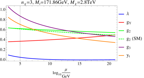
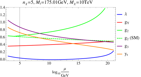
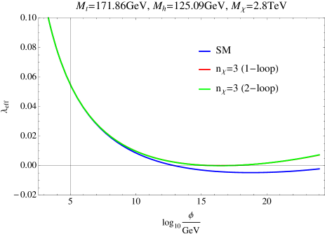
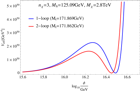
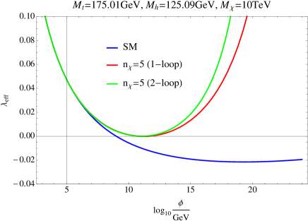
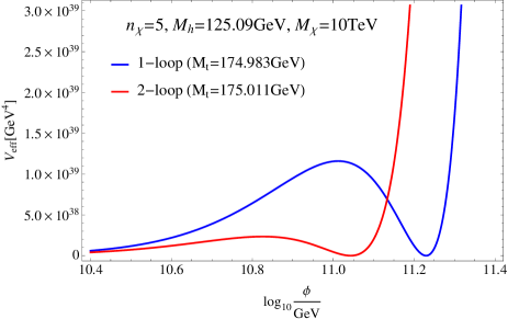
Figure 1: Upper left (right): the runnings of the SM parameters when $n_{\chi}=3$ $(5)$. Here, the dashed green lines represent the SM running of $g_{2}$. Middle (Lower): the running of the effective Higgs self coupling $\lambda_{\text{eff}}$ (left) and the one-loop effective Higgs potential $V_{\text{eff}}(\phi)$ (right) in the case of $n_{\chi}=3$ (5).

The upper panels of Fig.1 show the runnings of the SM parameters where $M_{h}=125.09$GeV, and $M_{t}$ is correspondingly fixed so that the MPP is realized. Here, we also show the SM running of $g_{2}$ by the dashed green line for comparison. Furthermore, in the middle and lower panels, we show the corresponding $\lambda_{\text{eff}}$ (left) and $V_{\text{eff}}(\phi)$ (right). In these figures, the one-loop results are also shown. One can actually see that the potential and its derivative simultaneously become zero at a high energy scale, and that the only triplet can have the other vacuum near the string/Planck scale. We note that the two-loop effects are small.

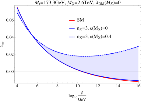
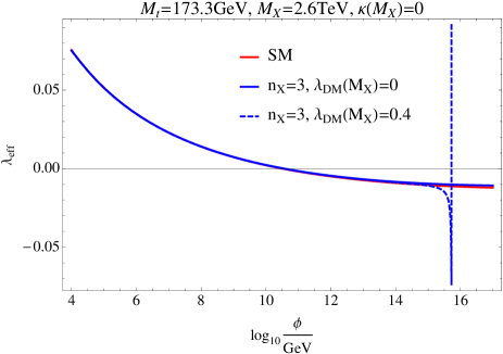
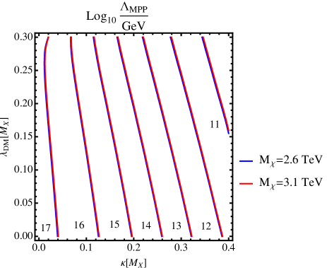
Figure 2: Upper: the running of $\lambda_{\text{eff}}$ in the case of $n_{X}=3$. Here, the blue band of the left panel corresponds to the change of $\kappa$ at $\mu=M_{X}$ from 0 to $0.4$. Lower: $\Lambda_{\text{MPP}}$ (left) and $M_{t}$ (right) as a function of $\kappa$ and $\lambda_{DM}$ at $\mu=M_{X}$. The blue (red) contours correspond to $M_{X}=2.6\hskip 2.84526pt(3.1)$ TeV.

Now let us consider a new scalar. As mentioned before, the remaining possibility is $n_{X}=3$ [69]. The potential of the scalar fields is

$$V=-\frac{M_{h}^{2}}{2}H^{\dagger}H+\frac{M_{X}^{2}}{2}XX+\lambda\left(H^{\dagger}H\right)^{2}+\lambda_{DM}\left(XX\right)^{2}+\kappa\left(H^{\dagger}H\right)\left(XX\right).$$ (4)

Here, $H$ is the SM Higgs doublet. The one-loop RGEs which are different from those of the SM are as follows:

$$\frac{dg_{2}}{dt} =-\frac{g_{2}^{3}}{(4\pi)^{2}}\frac{17}{6},$$ (5)

$$\frac{d\lambda}{dt} =\frac{1}{16\pi^{2}}\Bigg{(}\lambda\left(24\lambda-9g_{2}^{2}-3g_{Y}^{2}+12y_{t}^{2}\right)+\frac{3}{2}\kappa^{2}+\frac{3}{4}g_{Y}^{2}g_{2}^{2}+\frac{9}{8}g_{2}^{4}+\frac{3}{8}g_{Y}^{4}-6y_{t}^{4}\Bigg{)},$$ (6)

$$\frac{d\lambda_{DM}}{dt} =\frac{1}{16\pi^{2}}\left(22\lambda_{DM}^{2}+2\kappa^{2}-24g_{2}^{2}\lambda_{DM}+12g_{2}^{4}\right),$$ (7)

$$\frac{d\kappa}{dt} =\frac{1}{16\pi^{2}}\Bigg{(}4\kappa^{2}+12\kappa\lambda+10\kappa\lambda_{DM}+6y_{t}^{2}\kappa-\frac{33}{2}g_{2}^{2}\kappa-\frac{3}{2}g_{Y}^{2}\kappa+6g_{2}^{4}\Bigg{)}.$$ (8)

Furthermore, there is an additional contribution to $V_{\text{eff}}(\phi)$:

$$\Delta V_{\text{1loop}}(\phi)=\frac{3m_{DM}(\phi)^{4}}{64\pi^{2}}\left(\ln\left(\frac{m_{DM}(\phi)^{2}}{\phi^{2}}\right)-\frac{3}{2}\right),$$ (9)

where

$$m_{DM}(\phi)=\sqrt{M_{X}^{2}+\kappa(\phi)e^{2\Gamma(\phi)}\phi^{2}}.$$ (10)

In this case, the thermal abundance of $X$ depends on the value of $\kappa$. Here we use

$$M_{X}=2.6\hskip 5.69054pt\text{TeV and }3.1\hskip 5.69054pt\text{TeV}$$ (11)

for our calculation . $M_{X}=2.6$ TeV and $M_{X}=3.1$ TeV correspond to $\kappa=0$ and $\kappa=1$, respectively [68]. The upper panels of Fig.2 show the runnings of $\lambda_{\text{eff}}$ when $M_{X}=2.6$ TeV. Here, the blue band of the left panel corresponds to the change of $\kappa$ at $\mu=M_{X}$ from 0 to $0.4$. In the case of $\lambda_{DM}(M_{X})=0.4$ of the right panel, the rapid increase of $\lambda_{\text{eff}}$ around $10^{16}$ GeV is due to the Landau pole of $\lambda_{DM}$. Namely, $\lambda_{DM}$ becomes infinity below $M_{pl}$. The lower left (right) panel of Fig.3 shows the contour plot of $\Lambda_{\text{MPP}}\hskip 2.84526pt(M_{t})$ as a function of $\lambda_{DM}$ and $\kappa$ at $\mu=M_{X}$. The blue (red) contours correspond to $M_{X}=2.6\hskip 2.84526pt(3.1)$ TeV. One can see that $\Lambda_{\text{MPP}}$ is close to the string/Planck scale when $\kappa(M_{X})\lesssim 0.1$ and $M_{t}\lesssim 172$GeV.

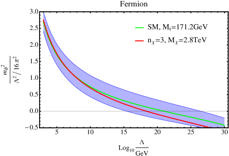
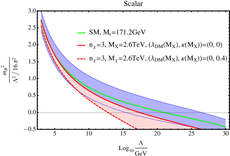
Figure 3: The bare Higgs mass $\frac{m_{B}^{2}}{16\pi^{2}\Lambda^{2}}$ as a function of a cut-off scale $\Lambda$. Here the blue bands (red band) correspond(s) to the $2\sigma$ deviation from $M_{t}=171.2$ GeV (the change of $\kappa$ at $\mu=M_{X}$ from 0 to $0.4$).

In order to discuss the Higgs potential around the cutoff scale $\Lambda$, it is meaningful to consider how the existence of a new particle changes the behavior of the bare Higgs mass $m_{B}$ as a function of $\Lambda$. This is because $m_{B}$ would appear in the Higgs potential above $\Lambda$ [31]. We now examine whether $m_{B}$ vanishes around the string scale or not. See [13] for the evaluation of $m_{B}$ in the SM.

Here, let us focus on $(n_{\chi(X)},Y_{\chi(X)})=(3,0)$ at one-loop level. For $\chi$, $m_{B}$ is given by

$$\frac{m_{B}^{2}|_{\text{1-loop}}}{\Lambda^{2}/16\pi^{2}}=-\left(6\lambda+{3\over 4}g_{Y}^{2}+{9\over 4}g_{2}^{2}-6y_{t}^{2}\right),$$ (12)

where the couplings are evaluated at $\mu=\Lambda$. On the other hand, for $X$, $m_{B}^{2}|_{\text{1-loop}}$ becomes

$$\frac{m_{B}^{2}|_{\text{1-loop}}}{\Lambda^{2}/16\pi^{2}}=-\left(6\lambda+{3\over 4}g_{Y}^{2}+{9\over 4}g_{2}^{2}-6y_{t}^{2}+\frac{3}{2}\kappa\right).$$ (13)

The left (right) panel of Fig.3 shows $m_{B}$ as a function of $\Lambda$ when a new particle is fermion (scalar). Here, the green contour is the SM prediction when $M_{t}=171.2$ GeV, and blue bands correspond to the $2\sigma$ deviation from it [73]:

$$M_{t}=171.2\pm 4.8\hskip 5.69054pt\text{GeV}\hskip 8.53581pt(95\%\text{CL}).$$ (14)

In the right panel, we change $\kappa$ at $\mu=M_{X}$ from 0 to 0.4, and they are represented by a red band. Depending on the values of $M_{t}$ and $\kappa$, one can see that the scale at which $m_{B}$ becomes zero quite changes. In both of cases, $m_{B}$ can take zero around the string scale . In addition to the vanishing $\lambda$ at around the string scale, this fact may suggest the MPP is realized at this scale.

In conclusion, we have studied the MPP of the SM with a weakly interacting new particle with its hypercharge being zero. When a new particle is a fermion, we have found that the top mass $M_{t}$ and $\Lambda_{\text{MPP}}$ can be uniquely predicted. On the other hand, when a new particle is scalar, there exists a new scalar coupling $\kappa$. Due to this coupling, we have found that $\Lambda_{\text{MPP}}$ and $M_{t}$ drastically change. In both of cases, only the triplets survive from the point of view that the other vacuum should exist around the string/Planck scale and that the theory is valid up to this scale. The analysis of this paper suggests that the SM and its triplet extensions are special in that the MPP can be realized around the string/Planck scale.

Appendix Appendix A Two-loop renormalization group equations and one-loop effective Higgs potential

The two-loop RGEs of the SM with a new fermion which is a $n_{\chi}$ representation of $SU(2)_{L}$ with the hypercharge $Y_{\chi}$ are as follows:

$$\frac{d\Gamma}{dt} =\frac{1}{(4\pi)^{2}}\left(\frac{9}{4}g_{2}^{2}+\frac{3}{4}g_{Y}^{2}-3y_{t}^{2}\right),$$ (15)

$$\frac{dg_{Y}}{dt} =\frac{g_{Y}^{3}}{(4\pi)^{2}}\left(\frac{41}{6}+\eta\hskip 2.84526ptn_{\chi}\frac{4}{3}Y_{\chi}^{2}\right)+\frac{g_{Y}^{3}}{(4\pi)^{4}}\left\{\left(\frac{199}{18}+4\eta\hskip 2.84526ptn_{\chi}Y_{\chi}^{4}\right)g_{Y}^{2}+\left(\frac{9}{2}+4\eta Y_{\chi}^{2}C_{n}\right)g_{2}^{2}+\frac{44}{3}g_{3}^{2}-\frac{17}{6}y_{t}^{2}\right\},$$ (16)

$$\frac{dg_{2}}{dt} =\frac{g_{2}^{3}}{(4\pi)^{2}}\left(-\frac{19}{6}+\eta\frac{4}{3}S_{n}\right)+\frac{g_{2}^{3}}{(4\pi)^{4}}\Biggl{\{}\left(\frac{3}{2}+\eta 4Y_{\chi}^{2}S_{n}\right)g_{Y}^{2}+\left(\frac{35}{6}+\eta\frac{40}{3}S_{n}+\eta 4C_{n}S_{n}\right)g_{2}^{2}+12g_{3}^{2}-\frac{3}{2}y_{t}^{2}\Biggl{\}},$$

$$\frac{dg_{3}}{dt} =-\frac{7}{(4\pi)^{2}}g_{3}^{3}+\frac{g_{3}^{3}}{(4\pi)^{4}}\left(\frac{11}{6}g_{Y}^{2}+\frac{9}{2}g_{2}^{2}-26g_{3}^{2}-2y_{t}^{2}\right),$$ (17)

$$\frac{dy_{t}}{dt} =\frac{y_{t}}{(4\pi)^{2}}\left(\frac{9}{2}y_{t}^{2}+3y_{\nu}^{2}-8g_{3}^{2}-\frac{9}{4}g_{2}^{2}-\frac{17}{12}g_{Y}^{2}\right)$$

$$+\frac{y_{t}}{(4\pi)^{4}}\Biggl{\{}\left(\frac{1187}{216}+\frac{29}{27}\eta\hskip 2.84526ptn_{\chi}Y_{\chi}^{2}\right)g_{Y}^{4}+\left(-\frac{23}{4}+\eta S_{n}\right)g_{2}^{4}-\frac{3}{4}g_{2}^{2}g_{Y}^{2}+\frac{19}{9}g_{3}^{2}g_{Y}^{2}+9g_{3}^{2}g_{2}^{2}-108g_{3}^{4}$$

$$\hskip 113.81102pt+\left(\frac{131}{16}g_{Y}^{2}+\frac{225}{16}g_{2}^{2}+36g_{3}^{2}\right)y_{t}^{2}+6\lambda^{2}-12\lambda y_{t}^{2}-12y_{t}^{4}\Biggl{\}},$$ (18)

$$\frac{d\lambda}{dt} =\frac{1}{16\pi^{2}}\Biggl{(}\lambda\left(24\lambda-9g_{2}^{2}-3g_{Y}^{2}+12y_{t}^{2}\right)+\frac{3}{4}g_{Y}^{2}g_{2}^{2}+\frac{9}{8}g_{2}^{4}+\frac{3}{8}g_{Y}^{4}-6y_{t}^{4}\Biggl{)}$$

$$+\frac{1}{(4\pi)^{4}}\Biggl{\{}-312\lambda^{3}+36\lambda^{2}\left(g_{Y}^{2}+3g_{2}^{2}\right)+\lambda\left(\frac{629}{24}g_{Y}^{4}+\frac{10}{3}Y_{\chi}^{2}g_{Y}^{4}-\frac{73}{8}g_{2}^{4}+10\eta S_{n}g_{2}^{4}+\frac{39}{4}g_{2}^{2}g_{Y}^{2}\right)$$

$$+\left(\frac{305}{16}-4\eta S_{n}\right)g_{2}^{6}-\left(\frac{289}{48}+\frac{4}{3}\eta S_{n}\right)g_{2}^{4}g_{Y}^{2}-\left(\frac{559}{48}+\frac{4}{3}\eta\hskip 2.84526ptn_{\chi}Y_{\chi}^{2}\right)g_{2}^{2}g_{Y}^{4}-\left(\frac{379}{48}+\frac{4}{3}n_{\chi}Y_{\chi}^{2}\right)g_{Y}^{6}$$

$$+\left(\frac{85}{6}g_{Y}^{2}+\frac{45}{2}g_{2}^{2}+80g_{3}^{2}\right)\lambda y_{t}^{2}+g_{Y}^{2}y_{t}^{2}\left(\frac{21}{2}g_{2}^{2}-\frac{19}{4}g_{Y}^{2}\right)-\frac{9}{4}g_{2}^{4}y_{t}^{2}-\frac{8}{3}g_{Y}^{2}y_{t}^{4}-32g_{3}^{2}y_{t}^{4}$$

$$-144\lambda^{2}y_{t}^{2}-3\lambda y_{t}^{4}+30y_{t}^{6}\Biggl{\}}.$$ (19)

Here, $t=\ln\mu$ with $\mu$ being the renormalization scale, $\Gamma$ is the wave function renormalization of the Higgs, $C_{n}$ and $S_{n}$ are the Casimir and Dynkin index, and $\eta=1,\frac{1}{2}$ for Dirac and Weyl fermion. The two-loop RGEs of $g_{Y}$ and $g_{2}$ are agreement with [51] by putting $y_{t}=0$.

The one-loop effective Higgs potential is

$$V_{\text{eff}}(\mu,\phi)=-\frac{M_{h}^{2}}{4}\phi^{2}+\frac{\lambda(\mu)}{4}\phi^{4}+V_{\text{1loop}}(\mu,\phi),$$ (20)

where

$$V_{\text{1-loop}}(\mu,\phi):=e^{4\Gamma(\mu)}\Biggl{\{}-12 \cdot\frac{M_{t}(\phi,\mu)^{4}}{64\pi^{2}}\left[\log\left(\frac{M_{t}(\phi,\mu)^{2}}{\mu^{2}}\right)-\frac{3}{2}+2\Gamma(\mu)\right]$$

$$+6\cdot\frac{M_{W}(\phi,\mu)^{4}}{64\pi^{2}}\left[\log\left(\frac{M_{W}(\phi,\mu)^{2}}{\mu^{2}}\right)-\frac{5}{6}+2\Gamma(\mu)\right]$$

$$+3\cdot\frac{M_{Z}(\phi,\mu)^{4}}{64\pi^{2}}\left[\log\left(\frac{M_{Z}(\phi,\mu)^{2}}{\mu^{2}}\right)-\frac{5}{6}+2\Gamma(\mu)\right]\Biggl{\}},$$ (21)

and

$$M_{t}(\phi,\mu)=\frac{y_{t}(\mu)}{\sqrt{2}}\phi\hskip 5.69054pt,\hskip 5.69054ptM_{W}(\phi,\mu)=\frac{g_{2}(\mu)}{2}\phi\hskip 5.69054pt,\hskip 5.69054ptM_{Z}(\phi,\mu)=\frac{\sqrt{g_{2}(\mu)^{2}+g_{Y}(\mu)^{2}}}{2}\phi.$$ (22)

In Eq.(21), we have neglected the contribution from the Higgs quartic term because it is small when we consider the MPP. In principle, $\mu$ should be determined as a function of $\phi$ so that $V_{\text{1-loop}}$ is minimized. However, in this paper, $\mu$ is taken to be $\phi$ for simplicity. It is known that this is a good approximation [44]. From $V_{\text{eff}}$, we define $\lambda_{\text{eff}}$ and $\beta_{\lambda_{\text{eff}}}$ as follows:

$$\lambda_{\text{eff}}(\phi):=\frac{4V_{\text{eff}}(\phi)}{\phi^{4}}\hskip 5.69054pt,\hskip 5.69054pt\beta_{\lambda_{\text{eff}}}(\phi):=\frac{d\lambda_{\text{eff}}(\phi)}{d\ln\phi}.$$ (23)

Appendix Appendix B Landau pole in septet and nonet fermion

As mentioned in the introduction, in cases of $n_{\chi}=7$ and $9$, there exists a scale $\Lambda_{LP}$ at which $g_{2}$ becomes infinity below $M_{pl}$, which is well known as the Landau Pole. Therefore, these theories are not favored from the point of view of perturbativity (triviality) up to the string/Planck scale. For completeness, we give numerical results of the Landau pole in Fig.4. Here, the two-loop results are shown by dashed lines. As is known, the one-loop Landau pole can be analytically solved:

$$\Lambda_{LP}|_{\text{1-loop}}=M_{\chi}\exp\left(\frac{8\pi^{2}}{\left(-\frac{19}{6}+\frac{1}{2}\frac{4}{3}S_{n}\right)g_{2}(M_{\chi})^{2}}\right),$$ (24)

where $S_{n}$ is the Dynkin index. From Fig.4, one can see that the two-loop effect is relatively important.

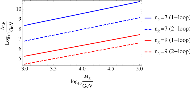
Figure 4: The scale $\Lambda_{LP}$ of the Landau pole as a function of $M_{\chi}$ when $n_{\chi}=7$ (blue) and $9$ (red). Here, the two-loop results are represented by dashed lines.

Appendix Appendix C New Fermion with $Y_{\chi}\neq 0$

Here, we consider a new fermion with $Y_{\chi}\neq 0$. As well as the real $n_{\chi}=7$ and 9 cases, the Landau pole of $g_{2}$ exists below $M_{pl}$ when $n_{\chi}\geq 5$ [51]. So, let us here focus on $n_{\chi}\leq 4$ . Here, we leave $M_{\chi}$ as a free parameter . The left (right) panel of Fig.5 shows $\Lambda_{\text{MPP}}$ $(M_{t})$ as a function of $M_{\chi}$ for each $(n_{\chi},Y_{\chi})$.

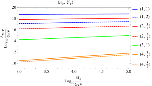
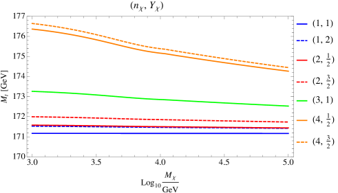
Figure 5: Left (Right): $\Lambda_{\text{MPP}}$ $(M_{t})$ as a function of $M_{\chi}$.

Appendix Appendix D Electroweak symmetry breaking by
Coleman-Weinberg mechanism

Here, we discuss a possibility to realize the electroweak symmetry breaking by the Coleman-Weinberg mechanism in the case of the SU(2) triplet scalar. The one-loop effective Higgs potential is

$$V(\mu,\phi)=\frac{\lambda(\mu)}{4}e^{4\Gamma(\mu)}\phi^{4} +\frac{3m_{DM}(\phi)^{4}}{64\pi^{2}}\left(\ln\left(\frac{m_{DM}(\phi)^{2}}{\mu^{2}}\right)-\frac{3}{2}\right)$$

$$+e^{4\Gamma(\mu)}\frac{(3\lambda(\mu)\phi^{2})^{2}}{64\pi^{2}}\left[\log\left(\frac{3\lambda(\mu)e^{2\Gamma(\mu)}\phi^{2}}{\mu^{2}}\right)-\frac{3}{2}\right]+\Delta V_{\text{1-loop}}(\mu,\phi),$$ (25)

where $m_{DM}(\phi)$ and $\Delta V_{\text{1-loop}}(\mu,\phi)$ are given by Eq.(10) and Eq.(21) respectively, and we have assumed that the quadratic term vanishes at the tree-level. In the following, we choose $\mu=m_{DM}(\phi)$. Then, $\phi$ develops the vacuum expectation value $v$ because the negative quadratic term appears from the second term in Eq.(25). The resultant vacuum expectation value is

$$v=\frac{3M_{X}}{4\pi}\sqrt{\frac{\kappa}{2\lambda}}\simeq 240\text{GeV}\left(\frac{M_{X}}{2.6\text{TeV}}\right)\times\sqrt{\frac{\kappa}{0.04}},$$ (26)

where we have neglected the 1-loop correction to the quartic term. It is interesting that the successful electroweak symmetry breaking is realized for $\kappa\simeq 0.04$ which is also favored by the MPP around the Planck scale.

References

- [1] G. Aad et al. [ATLAS Collaboration], “Observation of a new particle in the search for the Standard Model Higgs boson with the ATLAS detector at the LHC,” Phys. Lett. B 716, 1 (2012) [arXiv:1207.7214 [hep-ex]].
- [2] S. Chatrchyan et al. [CMS Collaboration], “Observation of a new boson at a mass of 125 GeV with the CMS experiment at the LHC,” Phys. Lett. B 716, 30 (2012) [arXiv:1207.7235 [hep-ex]].
- [3] C. D. Froggatt and H. B. Nielsen, “Standard model criticality prediction: Top mass 173 +- 5-GeV and Higgs mass 135 +- 9-GeV,” Phys. Lett. B 368, 96 (1996) [hep-ph/9511371].
- [4] C. D. Froggatt, H. B. Nielsen and Y. Takanishi, “Standard model Higgs boson mass from borderline metastability of the vacuum,” Phys. Rev. D 64, 113014 (2001) [hep-ph/0104161].
- [5] K. A. Meissner and H. Nicolai, “Conformal Symmetry and the Standard Model,” Phys. Lett. B 648, 312 (2007) [hep-th/0612165].
- [6] R. Foot, A. Kobakhidze, K. L. McDonald and R. R. Volkas, “A Solution to the hierarchy problem from an almost decoupled hidden sector within a classically scale invariant theory,” Phys. Rev. D 77 (2008) 035006 [arXiv:0709.2750 [hep-ph]].
- [7] K. A. Meissner and H. Nicolai, “Effective action, conformal anomaly and the issue of quadratic divergences,” Phys. Lett. B 660, 260 (2008) [arXiv:0710.2840 [hep-th]].
- [8] S. Iso, N. Okada and Y. Orikasa, “Classically conformal L extended Standard Model,” Phys. Lett. B 676 (2009) 81 [arXiv:0902.4050 [hep-ph]].
- [9] S. Iso, N. Okada and Y. Orikasa, “The minimal B-L model naturally realized at TeV scale,” Phys. Rev. D 80 (2009) 115007 [arXiv:0909.0128 [hep-ph]].
- [10] M. Shaposhnikov and C. Wetterich, “Asymptotic safety of gravity and the Higgs boson mass,” Phys. Lett. B 683, 196 (2010) [arXiv:0912.0208 [hep-th]].
- [11] M. Holthausen, K. S. Lim and M. Lindner, “Planck scale Boundary Conditions and the Higgs Mass,” JHEP 1202, 037 (2012) [arXiv:1112.2415 [hep-ph]].
- [12] F. Bezrukov, M. Y. Kalmykov, B. A. Kniehl and M. Shaposhnikov, “Higgs Boson Mass and New Physics,” JHEP 1210, 140 (2012) [arXiv:1205.2893 [hep-ph]].
- [13] Y. Hamada, H. Kawai and K. y. Oda, “Bare Higgs mass at Planck scale,” Phys. Rev. D 87, no. 5, 053009 (2013) [Phys. Rev. D 89, no. 5, 059901 (2014)] [arXiv:1210.2538 [hep-ph]].
- [14] S. Iso and Y. Orikasa, “TeV Scale B-L model with a flat Higgs potential at the Planck scale - in view of the hierarchy problem -,” PTEP 2013 (2013) 023B08 [arXiv:1210.2848 [hep-ph]].
- [15] H. B. Nielsen, “PREdicted the Higgs Mass,” arXiv:1212.5716 [hep-ph].
- [16] F. Jegerlehner, “The Standard model as a low-energy effective theory: what is triggering the Higgs mechanism?,” Acta Phys. Polon. B 45 (2014) 6, 1167 [arXiv:1304.7813 [hep-ph]].
- [17] F. Jegerlehner, “The hierarchy problem of the electroweak Standard Model revisited,” arXiv:1305.6652 [hep-ph].
- [18] Y. Hamada, H. Kawai and K. y. Oda, “Bare Higgs mass and potential at ultraviolet cutoff,” arXiv:1305.7055 [hep-ph].
- [19] D. Buttazzo, G. Degrassi, P. P. Giardino, G. F. Giudice, F. Sala, A. Salvio and A. Strumia, “Investigating the near-criticality of the Higgs boson,” JHEP 1312, 089 (2013) [arXiv:1307.3536 [hep-ph]].
- [20] V. Branchina and E. Messina, Phys. Rev. Lett. 111 (2013) 241801 [arXiv:1307.5193 [hep-ph]].
- [21] Y. Kawamura, “Naturalness, Conformal Symmetry and Duality,” PTEP 2013, no. 11, 113B04 (2013) [arXiv:1308.5069 [hep-ph]].
- [22] W. Chao, M. Gonderinger and M. J. Ramsey-Musolf, “Higgs Vacuum Stability, Neutrino Mass, and Dark Matter,” Phys. Rev. D 86, 113017 (2012) [arXiv:1210.0491 [hep-ph]].
- [23] A. Kobakhidze and A. Spencer-Smith, “The Higgs vacuum is unstable,” arXiv:1404.4709 [hep-ph].
- [24] N. Khan and S. Rakshit, “Study of electroweak vacuum metastability with a singlet scalar dark matter,” Phys. Rev. D 90, no. 11, 113008 (2014) [arXiv:1407.6015 [hep-ph]].
- [25] N. Khan and S. Rakshit, “Constraints on inert dark matter from metastability of electroweak vacuum,” arXiv:1503.03085 [hep-ph].
- [26] A. Spencer-Smith, “Higgs Vacuum Stability in a Mass-Dependent Renormalisation Scheme,” arXiv:1405.1975 [hep-ph].
- [27] N. Haba, H. Ishida, K. Kaneta and R. Takahashi, “Vanishing Higgs potential at the Planck scale in a singlet extension of the standard model,” Phys. Rev. D 90, 036006 (2014) [arXiv:1406.0158 [hep-ph]].
- [28] R. Foot, A. Kobakhidze and A. Spencer-Smith, “Criticality in the scale invariant standard model (squared),” Phys. Lett. B 747 (2015) 169 [arXiv:1409.4915 [hep-ph]].
- [29] I. Oda, “Conformal Higgs Gravity,” arXiv:1505.06760 [gr-qc].
- [30] F. L. Bezrukov and M. Shaposhnikov, “The Standard Model Higgs boson as the inflaton,” Phys. Lett. B 659, 703 (2008) [arXiv:0710.3755 [hep-th]].
- [31] Y. Hamada, H. Kawai and K. y. Oda, “Minimal Higgs inflation,” PTEP 2014, 023B02 (2014) [arXiv:1308.6651 [hep-ph]].
- [32] F. Jegerlehner, “Higgs inflation and the cosmological constant,” Acta Phys. Polon. B 45 (2014) 6, 1215 [arXiv:1402.3738 [hep-ph]].
- [33] Y. Hamada, H. Kawai, K. y. Oda and S. C. Park, “Higgs inflation still alive,” Phys. Rev. Lett. 112, 241301 (2014) [arXiv:1403.5043 [hep-ph]].
- [34] M. Fairbairn and R. Hogan, “Electroweak Vacuum Stability in light of BICEP2,” Phys. Rev. Lett. 112, 201801 (2014) [arXiv:1403.6786 [hep-ph]].
- [35] F. Bezrukov and M. Shaposhnikov, “Higgs inflation at the critical point,” Phys. Lett. B 734 (2014) 249 [arXiv:1403.6078 [hep-ph]].
- [36] K. Enqvist, T. Meriniemi and S. Nurmi, “Higgs Dynamics during Inflation,” JCAP 1407 (2014) 025 [arXiv:1404.3699 [hep-ph]].
- [37] A. Hook, J. Kearney, B. Shakya and K. M. Zurek, “Probable or Improbable Universe? Correlating Electroweak Vacuum Instability with the Scale of Inflation,” JHEP 1501, 061 (2015) [arXiv:1404.5953 [hep-ph]].
- [38] N. Haba and R. Takahashi, “Higgs inflation with singlet scalar dark matter and right-handed neutrino in light of BICEP2,” Phys. Rev. D 89 (2014) 11, 115009 [Phys. Rev. D 90 (2014) 3, 039905] [arXiv:1404.4737 [hep-ph]].
- [39] Y. Hamada, H. Kawai and K. y. Oda, “Predictions on mass of Higgs portal scalar dark matter from Higgs inflation and flat potential,” JHEP 1407, 026 (2014) [arXiv:1404.6141 [hep-ph]].
- [40] P. Ko and W. I. Park, “Higgs-portal assisted Higgs inflation with a large tensor-to-scalar ratio,” arXiv:1405.1635 [hep-ph].
- [41] N. Haba, H. Ishida and R. Takahashi, “Higgs inflation and Higgs portal dark matter with right-handed neutrinos,” PTEP 2015 (2015) 5, 053B01 [arXiv:1405.5738 [hep-ph]].
- [42] H. J. He and Z. Z. Xianyu, “Extending Higgs Inflation with TeV Scale New Physics,” JCAP 1410 (2014) 019 [arXiv:1405.7331 [hep-ph]].
- [43] M. Herranen, T. Markkanen, S. Nurmi and A. Rajantie, “Spacetime curvature and the Higgs stability during inflation,” Phys. Rev. Lett. 113, no. 21, 211102 (2014) [arXiv:1407.3141 [hep-ph]].
- [44] Y. Hamada, H. Kawai, K. y. Oda and S. C. Park, “Higgs inflation from Standard Model criticality,” Phys. Rev. D 91 (2015) 5, 053008 [arXiv:1408.4864 [hep-ph]].
- [45] Y. Hamada, K. y. Oda and F. Takahashi, “Topological Higgs inflation: Origin of Standard Model criticality,” Phys. Rev. D 90 (2014) 9, 097301 [arXiv:1408.5556 [hep-ph]].
- [46] Y. Hamada, H. Kawai and K. y. Oda, “Eternal Higgs inflation and cosmological constant problem,” arXiv:1501.04455 [hep-ph].
- [47] N. Okada and Q. Shafi, “Higgs Inflation, Seesaw Physics and Fermion Dark Matter,” Phys. Lett. B 747, 223 (2015) [arXiv:1501.05375 [hep-ph]].
- [48] T. Inagaki, R. Nakanishi and S. D. Odintsov, “Non-Minimal Two-Loop Inflation,” Phys. Lett. B 745 (2015) 105 [arXiv:1502.06301 [hep-ph]].
- [49] F. Jegerlehner, “The hierarchy problem and the cosmological constant problem in the Standard Model,” arXiv:1503.00809 [hep-ph].
- [50] Y. Abe, T. Inami, Y. Kawamura and Y. Koyama, “Inflation from radion gauge-Higgs potential at Planck scale,” arXiv:1504.06905 [hep-th].
- [51] L. Di Luzio, R. Grober, J. F. Kamenik and M. Nardecchia, “Accidental matter at the LHC,” arXiv:1504.00359 [hep-ph].
- [52] K. Bamba, S. D. Odintsov and P. V. Tretyakov, “Inflation in a conformally-invariant two-scalar-field theory with an extra term,” arXiv:1505.00854 [hep-th].
- [53] S. Nurmi, T. Tenkanen and K. Tuominen, “Inflationary Imprints on Dark Matter,” arXiv:1506.04048 [astro-ph.CO].
- [54] L. Sebastiani and R. Myrzakulov, “F(R) gravity and inflation,” arXiv:1506.05330 [gr-qc].
- [55] M. Herranen, T. Markkanen, S. Nurmi and A. Rajantie, “Spacetime curvature and Higgs stability after inflation,” arXiv:1506.04065 [hep-ph].
- [56] H. Kawai and T. Okada, “Solving the Naturalness Problem by Baby Universes in the Lorentzian Multiverse,” Prog. Theor. Phys. 127, 689 (2012) [arXiv:1110.2303 [hep-th]].
- [57] H. Kawai, “Low energy effective action of quantum gravity and the naturalness problem,” Int. J. Mod. Phys. A 28, 1340001 (2013).
- [58] Y. Hamada, H. Kawai and K. Kawana, “Evidence of the Big Fix,” Int. J. Mod. Phys. A 29, no. 17, 1450099 (2014) [arXiv:1405.1310 [hep-ph]].
- [59] Y. Hamada, H. Kawai and K. Kawana, “Weak Scale From the Maximum Entropy Principle,” PTEP 2015 (2015) 3, 033B06 [arXiv:1409.6508 [hep-ph]].
- [60] Y. Hamada, H. Kawai and K. Kawana, “Saddle point inflation in string-inspired theory,” PTEP 2015, 091B01 (2015) [arXiv:1507.03106 [hep-ph]].
- [61] Y. Hamada, H. Kawai and K. Kawana, “Natural solution to the naturalness problem – Universe does fine-tuning,” arXiv:1509.05955 [hep-th].
- [62] K. Kawana, “Multiple Point Principle of the Standard Model with Scalar Singlet Dark Matter and Right Handed Neutrinos,” PTEP 2015, no. 2, 023B04 [arXiv:1411.2097 [hep-ph]].
- [63] H. Okada and Y. Orikasa, “Classically Conformal Radiative Neutrino Model with Gauged B-L Symmetry,” arXiv:1412.3616 [hep-ph].
- [64] K. Kawana, “Criticality and Inflation of the Gauged B-L Model,” arXiv:1501.04482 [hep-ph].
- [65] N. Haba and Y. Yamaguchi, “Vacuum stability in the extended model with vanishing scalar potential at the Planck scale,” arXiv:1504.05669 [hep-ph].
- [66] M. Cirelli, N. Fornengo and A. Strumia, “Minimal dark matter,” Nucl. Phys. B 753, 178 (2006) [hep-ph/0512090].
- [67] J. Hisano, S. Matsumoto, M. Nagai, O. Saito and M. Senami, “Non-perturbative effect on thermal relic abundance of dark matter,” Phys. Lett. B 646, 34 (2007) [hep-ph/0610249].
- [68] M. Cirelli, A. Strumia and M. Tamburini, “Cosmology and Astrophysics of Minimal Dark Matter,” Nucl. Phys. B 787, 152 (2007) [arXiv:0706.4071 [hep-ph]].
- [69] Y. Hamada, K. Kawana and K. Tsumura, “Landau pole in the Standard Model with weakly interacting scalar fields,” Phys. Lett. B 747, 238 (2015) [arXiv:1505.01721 [hep-ph]].
- [70] G. Aad et al. [ATLAS and CMS Collaborations], “Combined Measurement of the Higgs Boson Mass in Collisions at and 8 TeV with the ATLAS and CMS Experiments,” Phys. Rev. Lett. 114, 191803 (2015) [arXiv:1503.07589 [hep-ex]].
- [71] [ATLAS and CDF and CMS and D0 Collaborations], “First combination of Tevatron and LHC measurements of the top-quark mass,” arXiv:1403.4427 [hep-ex].
- [72] CMS Collaboration [CMS Collaboration], “Combination of the CMS top-quark mass measurements from Run 1 of the LHC,” CMS-PAS-TOP-14-015.
- [73] S. Moch, S. Weinzierl, S. Alekhin, J. Blumlein, L. de la Cruz, S. Dittmaier, M. Dowling and J. Erler et al., “High precision fundamental constants at the TeV scale,” arXiv:1405.4781 [hep-ph].
- [74] M. J. G. Veltman, “The Infrared - Ultraviolet Connection,” Acta Phys. Polon. B 12 (1981) 437.
- [75] M. E. Machacek and M. T. Vaughn, “Two Loop Renormalization Group Equations in a General Quantum Field Theory. 1. Wave Function Renormalization,” Nucl. Phys. B 222, 83 (1983).
- [76] M. E. Machacek and M. T. Vaughn, “Two Loop Renormalization Group Equations in a General Quantum Field Theory. 2. Yukawa Couplings,” Nucl. Phys. B 236, 221 (1984).
- [77] M. E. Machacek and M. T. Vaughn, “Two Loop Renormalization Group Equations in a General Quantum Field Theory. 3. Scalar Quartic Couplings,” Nucl. Phys. B 249, 70 (1985).
- [78] M. x. Luo, H. w. Wang and Y. Xiao, “Two loop renormalization group equations in general gauge field theories,” Phys. Rev. D 67, 065019 (2003) [hep-ph/0211440].