Partial dynamical symmetry in Bose-Fermi systems

Abstract

We generalize the notion of partial dynamical symmetry (PDS) to a system of interacting bosons and fermions. In a PDS, selected states of the Hamiltonian are solvable and preserve the symmetry exactly, while other states are mixed. As a first example of such novel symmetry construction, spectral features of the odd-mass nucleus ¹⁹⁵Pt are analyzed.

During the last several decades, the concept of dynamical symmetry (DS) has become the cornerstone of algebraic modeling of dynamical systems. It has been applied in many branches of physics, such as hadronic BNB , nuclear ibm ; ibfm , atomic nano and molecular physics vibron ; Frank94 . Its basic paradigm is to write the Hamiltonian of the system in terms of Casimir operators of a chain of nested algebras, $G_{\rm dyn}\supset G\supset\dots\supset G_{\rm sym}$, where $G_{\rm dyn}$ is the dynamical algebra, in terms of which any model operator of a physical observable can be expressed, and $G_{\rm sym}$ is the symmetry algebra. A given DS defines a class of many-body Hamiltonians that admit an analytic solution for all states, with closed expressions for the energy eigenvalues, quantum numbers for classification and definite selection rules for transition processes.

An exact DS provides considerable insights into complex dynamics and its merits are self evident. However, in most applications to realistic systems, its predictions are rarely fulfilled and one is compelled to break it. The DS spectrum imposes constraints on the pattern of level-splitting which many times is at variance with the empirical data. More often one finds that the assumed symmetry is not obeyed uniformly, i.e., is fulfilled by some of the states but not by others. The required symmetry breaking is achieved by including in the Hamiltonian terms associated with different subalgebra chains of $G_{\rm dyn}$, resulting in a loss of solvability and pronounced mixing. The need to address such situations, but still preserve important symmetry remnants, has led to the introduction of partial dynamical symmetry (PDS) Alhassid92 ; Leviatan96 . The essential idea is to relax the stringent conditions of complete solvability so that only part of the eigenspectrum retains analyticity and/or good quantum numbers, in the spirit of quasi-solvable models QSM . Various types of PDSs were proposed Leviatan96 ; Leviatan86 ; Isacker99 ; Leviatan02 ; Leviatan11 and algorithms for constructing Hamiltonians with such property have been developed Alhassid92 ; GarciaRamos09 . Bosonic Hamiltonians with PDS have been applied to nuclear spectroscopy Leviatan96 ; Leviatan86 ; Isacker99 ; Leviatan02 ; Leviatan11 ; GarciaRamos09 ; Leviatan13 ; Casten14 ; Kremer14 , where extensive tests provide empirical evidence for their relevance to a broad range of nuclei. Similar PDS Hamiltonians have been used in molecular spectroscopy Ping97 and in the study of quantum phase transitions Leviatan07 ; Macek14 and of mixed regular and chaotic dynamics Macek14 ; WAL93 . Fermionic Hamiltonians with PDS have been identified within the nuclear shell model and applied to light nuclei Escher00 and seniority isomers Rowe01 ; Isacker08 . The growing number of empirical manifestations suggests a more pervasive role of PDSs in dynamical systems than heretofore realized.

All examples of PDS considered so far, were confined to systems of a given statistics (bosons or fermions). In this Rapid Communication, we extend the PDS concept to mixed systems of bosons and fermions, and present an empirical example of this novel construction. Systems with such composition of constituents are of broad interest and arise, for example, in the study of rotation-vibration-electronic spectra in molecules, collective states in odd-mass nuclei, electron-phonon phenomena in crystals, and spin-boson models in quantum optics.

If the separate numbers of bosons $N$ and fermions $M$ are conserved, the dynamical algebra of a Bose-Fermi system is of product form

$$\begin{array}[]{ccc}{\rm U}^{\rm B}(\Omega_{\rm B})&\otimes&{\rm U}^{\rm F}(\Omega_{\rm F})\\ \downarrow&&\downarrow\\[0.0pt] [N]&&[1^{M}]\end{array},$$ (1)

where $\Omega_{\rm B}$ ($\Omega_{\rm F}$) is the number of states available to a single boson (fermion). The statistics among the particles is imposed by an appropriate choice of irreducible representation (irrep), symmetric and anti-symmetric, for the bosons and fermions, respectively, as indicated in Eq. (1). There exist several strategies to define DSs with ${\rm U}^{\rm B}(\Omega_{\rm B})\otimes{\rm U}^{\rm F}(\Omega_{\rm F})$ as a starting point ibfm . They all define a chain of nested subalgebras, relying on the existence of isomorphisms between boson and fermion algebras and ending in the symmetry algebra.

Let us for the sake of concreteness consider a particular example while emphasizing that results of this Rapid Communication are of a generic nature that apply to any quantum-mechanical problem of interacting bosons and fermions, as long as it can be formulated in an algebraic language. We consider $N$ bosons with angular momentum $\ell=0$ ($s$) or $\ell=2$ ($d$) coupled to a single ($M=1$) fermion with angular momentum $j=1/2$, 3/2, or 5/2. This corresponds to the choice $\Omega_{\rm B}=6$ and $\Omega_{\rm F}=12$, and a possible classification is as follows:

$$\begin{array}[]{ccccc ccccccccc c}{\rm U}^{\rm B}(6)&\otimes&{\rm U}^{\rm F}(12)&\supset&\Big{(}{\rm U}^{\rm BF}(6)&\supset&{\rm SO}^{\rm BF}(6)&\supset&{\rm SO}^{\rm BF}(5)&\supset&{\rm SO}^{\rm BF}(3)\Big{)}&\otimes&{\rm SU}^{\rm F}(2)&\supset&{\rm Spin}^{\rm BF}(3)\\ \downarrow&&\downarrow&&\downarrow&&\downarrow&&\downarrow&&\downarrow&&\downarrow&&\downarrow\\[0.0pt] [N]&&[1^{M}]&&[N_{1},N_{2}]&&\langle\sigma_{1},\sigma_{2}\rangle&&(\tau_{1},\tau_{2})&&L&&\tilde{s}&&J\end{array},$$ (2)

where underneath each algebra the associated irrep labels are indicated, and $G^{\rm BF}$ is the direct sum of $G^{\rm B}$ and $G^{\rm F}$. For $M=0$, the classification (2) reduces to the SO(6) limit of the interacting boson model Arima79 which is of relevance for the even-even platinum isotopes Cizewski78 . For $M=1$, the classification (2) is proposed in the context of the interacting boson-fermion model (IBFM) ibfm to describe odd-mass isotopes of platinum with the odd neutron in the orbits $3p_{1/2}$, $3p_{3/2}$, and $2f_{5/2}$, which are dominant for these isotopes Isacker84 ; Bijker85 . Since we are interested here in Bose-Fermi systems, we apply the classification (2) for $M=1$, which implies $\tilde{s}=1/2$, and refer to it as the ${\rm SO}^{\rm BF}(6)$ limit.

The eigenstates (2) are obtained with a Hamiltonian that is a combination of Casimir operators $\hat{C}_{n}[G]$ of order $n$ of an algebra $G$ appearing in the chain. Up to a constant energy, this Hamiltonian is of the form

$$\hat{H}_{\rm DS} = a\,\hat{C}_{2}[{\rm U}^{\rm BF}(6)]+b\,\hat{C}_{2}[{\rm SO}^{\rm BF}(6)]+c\,\hat{C}_{2}[{\rm SO}^{\rm BF}(5)]$$ (3)

$$+d\,\hat{C}_{2}[{\rm SO}^{\rm BF}(3)]+d^{\prime}\hat{C}_{2}[{\rm Spin}^{\rm BF}(3)].$$

The associated eigenvalue problem is analytically solvable, leading to the energy expression

$$E_{\rm DS} = a\,f_{5}(N_{1},N_{2})+b\,f_{4}(\sigma_{1},\sigma_{2})+c\,f_{3}(\tau_{1},\tau_{2})$$ (4)

$$+d\,L(L+1)+d^{\prime}J(J+1),$$

with $f_{i}(s_{1},s_{2})\equiv s_{1}(s_{1}+i)+s_{2}(s_{2}+i-2)$. The energy spectrum of the Hamiltonian (3) is then determined once the allowed values of $[N_{1},N_{2}]$, $\langle\sigma_{1},\sigma_{2}\rangle$, $(\tau_{1},\tau_{2})$, $L$, and $J$ for a given $N$ and $M=1$ are found. Such branching rules can be obtained with standard group-theoretical techniques Wybourne74 .

Table 1: Two-particle tensor operators in the ${\rm SO}^{\rm BF}(6)$ limit. The superscript ${\cal L}({\cal J})$ stands for the coupling ${\cal J}={\cal L}\pm 1/2$.

$N$	$M$	$[N_{1},N_{2}]$	$\langle\sigma_{1},\sigma_{2}\rangle$	$(\tau_{1},\tau_{2})$	${\cal L}$	${\cal J}$		Tensor operator ${\cal T}^{{\cal L}({\cal J})}_{+,M_{\cal J}}$
$2$	$0$	$[2,0]$	$\langle 0,0\rangle$	$(0,0)$	$0$	$0$		${\cal V}^{0(0)}_{+}\equiv\sqrt{\frac{5}{12}}(d^{\dagger}d^{\dagger})^{(0)}_{0}-\sqrt{\frac{1}{12}}(s^{\dagger}s^{\dagger})^{(0)}_{0}$
$1$	$1$	$[2,0]$	$\langle 0,0\rangle$	$(0,0)$	$0$	$1/2$		${\cal V}^{0(1/2)}_{+,\mu}\equiv-\sqrt{\frac{1}{6}}(s^{\dagger}a^{\dagger}_{1/2})^{(1/2)}_{\mu}-\sqrt{\frac{1}{3}}(d^{\dagger}a^{\dagger}_{3/2})^{(1/2)}_{\mu}+\sqrt{\frac{1}{2}}(d^{\dagger}a^{\dagger}_{5/2})^{(1/2)}_{\mu}$
$1$	$1$	$[1,1]$	$\langle 1,1\rangle$	$(1,1)$	$1$	$1/2$		${\cal U}^{1(1/2)}_{+,\mu}\equiv\sqrt{\frac{3}{5}}(d^{\dagger}a^{\dagger}_{3/2})^{(1/2)}_{\mu}+\sqrt{\frac{2}{5}}(d^{\dagger}a^{\dagger}_{5/2})^{(1/2)}_{\mu}$
$1$	$1$	$[1,1]$	$\langle 1,1\rangle$	$(1,1)$	$1$	$3/2$		${\cal U}^{1(3/2)}_{+,\mu}\equiv-\sqrt{\frac{3}{10}}(d^{\dagger}a^{\dagger}_{3/2})^{(3/2)}_{\mu}+\sqrt{\frac{7}{10}}(d^{\dagger}a^{\dagger}_{5/2})^{(3/2)}_{\mu}$
$1$	$1$	$[1,1]$	$\langle 1,1\rangle$	$(1,0)$	$2$	$3/2$		${\cal U}^{2(3/2)}_{+,\mu}\equiv\sqrt{\frac{1}{2}}(s^{\dagger}a^{\dagger}_{3/2})^{(3/2)}_{\mu}-\sqrt{\frac{1}{2}}(d^{\dagger}a^{\dagger}_{1/2})^{(3/2)}_{\mu}$
$1$	$1$	$[1,1]$	$\langle 1,1\rangle$	$(1,0)$	$2$	$5/2$		${\cal U}^{2(5/2)}_{+,\mu}\equiv\sqrt{\frac{1}{2}}(s^{\dagger}a^{\dagger}_{5/2})^{(5/2)}_{\mu}-\sqrt{\frac{1}{2}}(d^{\dagger}a^{\dagger}_{1/2})^{(5/2)}_{\mu}$
$1$	$1$	$[1,1]$	$\langle 1,1\rangle$	$(1,1)$	$3$	$5/2$		${\cal U}^{3(5/2)}_{+,\mu}\equiv\sqrt{\frac{4}{5}}(d^{\dagger}a^{\dagger}_{3/2})^{(5/2)}_{\mu}+\sqrt{\frac{1}{5}}(d^{\dagger}a^{\dagger}_{5/2})^{(5/2)}_{\mu}$
$1$	$1$	$[1,1]$	$\langle 1,1\rangle$	$(1,1)$	$3$	$7/2$		${\cal U}^{3(7/2)}_{+,\mu}\equiv-\sqrt{\frac{1}{10}}(d^{\dagger}a^{\dagger}_{3/2})^{(7/2)}_{\mu}+\sqrt{\frac{9}{10}}(d^{\dagger}a^{\dagger}_{5/2})^{(7/2)}_{\mu}$

While $\hat{H}_{\rm DS}$ (3) is completely solvable, the question arises whether terms can be added that preserve solvability for part of its spectrum. This can be achieved by the construction of a PDS.

The algorithm to construct a PDS GarciaRamos09 starts from the character under the classification (2) of the boson and fermion creation operators $b^{\dagger}_{\ell m_{\ell}}$ and $a^{\dagger}_{jm_{j}}$ ibfm . Annihilation operators $b_{\ell m_{\ell}}$ and $a_{jm_{j}}$ transform in the same manner under orthogonal algebras if they are modified according to $\tilde{b}_{\ell m_{\ell}}\equiv(-)^{\ell+m_{\ell}}b_{\ell,-m_{\ell}}$ and $\tilde{a}_{jm_{j}}\equiv(-)^{j+m_{j}}a_{j,-m_{j}}$. The single-fermion angular momentum ($j=1/2,3/2,5/2$) can be divided into a pseudo-orbital angular momentum $(\tilde{\ell}\!=\!0,2)$ coupled to a pseudo-spin ($\tilde{s}\!=\!1/2$). The resulting $\tilde{\ell}$-$\tilde{s}$ basis is given by $c^{{\dagger}}_{\tilde{\ell}\tilde{m}_{\ell};\tilde{s}\tilde{m}_{s}}=\sum_{j,m}(\tilde{\ell},\tilde{m}_{\ell};\tilde{s},\tilde{m}_{s}|j,m)\,a^{\dagger}_{jm}$.

Composite operators with definite tensor character under the classification (2) can be constructed by use of generalized coupling coefficients which can be written as a product of ${\rm U}(6)\supset{\rm SO}(6)$, ${\rm SO}(6)\supset{\rm SO}(5)$, and ${\rm SO}(5)\supset{\rm SO}(3)$ isoscalar factors Wybourne74 . For the two-particle operators (needed for the construction of a two-body interaction) the tensor character is uniquely specified by the SO(6) and SO(5) labels $\langle\sigma_{1},\sigma_{2}\rangle$ and $(\tau_{1},\tau_{2})$, together with the SO^BF(3) and Spin^BF(3) labels $\cal L$ and $\cal J$. For example, operators that create a boson and a fermion with tensor character $[N_{1},N_{2}]$ $\langle\sigma_{1},\sigma_{2}\rangle$ $(\tau_{1},\tau_{2})$ ${\cal LJ}$ are

$$\sum_{\tau\tilde{\tau}}\left\langle\begin{array}[]{cc|c}\langle 1\rangle&\langle 1\rangle&\langle\sigma_{1},\sigma_{2}\rangle\\ (\tau)&(\tilde{\tau})&(\tau_{1},\tau_{2})\end{array}\right\rangle\sum_{j}\bar{\cal L}\bar{\jmath}\Bigl{\{}\begin{array}[]{ccc}\ell&\tilde{\ell}&{\cal L}\\ \tilde{s}&{\cal J}&j\end{array}\Bigr{\}}(b^{\dagger}_{\ell}a^{\dagger}_{j})^{({\cal J})}_{M_{\cal J}},$$

with $(\ell,\tilde{\ell})=0,2$, for $(\tau,\tilde{\tau})=0,1$, respectively, $j\!=\!\tilde{\ell}\pm 1/2$, $\bar{x}\equiv\sqrt{2x+1}$ and the symbol $\left\langle:\,:|:\right\rangle$ is an ${\rm SO}(6)\supset{\rm SO}(5)$ isoscalar factor, tabulated in Ref. ibfm . Expressions for the two-particle creation operators of interest here are given in Table 1. The corresponding annihilation operators with the correct tensor properties follow from $\tilde{\cal T}^{{\cal L}({\cal J})}_{-,M_{\cal J}}\!=\!(-)^{{\cal J}+M_{\cal J}}\left({\cal T}^{{\cal L}({\cal J})}_{+,-M_{\cal J}}\right)^{\dagger}$, where ${\cal T}\!=\!{\cal U}$ or $\cal V$.

The lowest-lying states in the spectrum of an odd-mass nucleus, described in terms of $N$ bosons and one fermion, can be written as $|[N+1]\langle N+1\rangle(\tau)LJM_{J}\rangle$; the next class of states belongs to $|[N,1]\langle N,1\rangle(\tau_{1},\tau_{2})LJM_{J}\rangle$ while there is also some evidence from one-neutron transfer for $|[N,1]\langle N-1\rangle(\tau)LJM_{J}\rangle$ states Metz00 . All two-particle operators listed in Table 1 annihilate particular states, hence lead to a PDS of some kind. For example, the operators with ${\rm U}^{\rm BF}(6)$ labels $[N_{1},N_{2}]=[1,1]$ satisfy

$$\tilde{\cal U}^{{\cal L}({\cal J})}_{-,M_{\cal J}}|[N+1]\langle\sigma\rangle(\tau)LJM_{J}\rangle=0,$$ (5)

for all permissible $(\sigma\tau LJM_{J})$. This is so because a state with $N-1$ bosons and no fermion has the ${\rm U}^{\rm BF}(6)$ label $[N-1]$. Given the multiplication $[N-1]\otimes[1,1]=[N,1]\oplus[N-1,1,1]$, the action of a ${\cal U}^{{\cal L}({\cal J})}_{+,-M_{\cal J}}$ operator on an $(N-1)$-boson state can never yield a boson-fermion state with the ${\rm U}^{\rm BF}(6)$ labels $[N+1]$. Similar arguments involving SO(6) multiplication lead to the following properties for the $\cal V$ operators which have SO(6) tensor character $\langle 0,0\rangle$:

$$\tilde{\cal V}^{0({\cal J})}_{-,M_{\cal J}}|[N+1]\langle N+1\rangle(\tau)LJM_{J}\rangle=0,$$ (6a)

$$\tilde{\cal V}^{0({\cal J})}_{-,M_{\cal J}}|[N,1]\langle N,1\rangle(\tau_{1},\tau_{2})LJM_{J}\rangle=0.$$ (6b)

An alternative way of constructing Hamiltonians with PDS for an algebra $G$, is to identify $n$-particle operators which annihilate a lowest-weight state of a prescribed $G$-irrep Alhassid92 . In the IBFM, such a state, which transforms as $[N+1]$ and $\tilde{s}=1/2$ under ${\rm U}^{\rm BF}(6)\otimes{\rm SU}^{\rm F}(2)$, is given by

$$|\Psi_{\rm g}\rangle\propto[b^{{\dagger}}_{c}(\beta)]^{N}f^{{\dagger}}_{\tilde{m}_{s}}(\beta)|0\rangle,$$ (7)

where $b^{{\dagger}}_{c}(\beta)\propto(\beta\,d^{{\dagger}}_{0}+s^{{\dagger}})$ and $f^{{\dagger}}_{\tilde{m}_{s}}(\beta)\propto(\beta\,c^{{\dagger}}_{2,0;1/2,\tilde{m}_{s}}+c^{{\dagger}}_{0,0;1/2,\tilde{m}_{s}})$ in the $\tilde{\ell}$-$\tilde{s}$ basis defined above. $|\Psi_{\rm g}\rangle$ is a condensate of $N$ bosons and a single fermion, and represents an intrinsic state for the ground band with deformation $\beta$. The Hermitian conjugate of the following two-particle operators

$${\cal V}^{0(0)}_{+} = {\textstyle\sqrt{\frac{5}{12}}}(d^{\dagger}d^{\dagger})^{(0)}_{0}-{\textstyle\frac{\beta^{2}}{\sqrt{12}}}(s^{\dagger}s^{\dagger})^{(0)}_{0},$$ (8a)

$${\cal V}^{0(1/2)}_{+,\mu} = \sqrt{\tfrac{5}{6}}(d^{{\dagger}}c^{{\dagger}}_{2;1/2})^{0(1/2)}_{\mu}-\tfrac{\beta^{2}}{\sqrt{6}}(s^{{\dagger}}c^{{\dagger}}_{0;1/2})^{0(1/2)}_{\mu},\qquad$$ (8b)

$${\cal U}^{{\cal L}({\cal J})}_{+,\mu} = (d^{{\dagger}}c^{{\dagger}}_{2;1/2})^{{\cal L}({\cal J})}_{\mu},\quad{\textstyle{\cal L}=1,3},$$ (8c)

$${\cal U}^{2({\cal J})}_{+,\mu} = (s^{{\dagger}}c^{{\dagger}}_{2;1/2})^{2({\cal J})}_{\mu}-(d^{{\dagger}}c^{{\dagger}}_{0;1/2})^{2({\cal J})}_{\mu},$$ (8d)

satisfy $\tilde{\cal T}^{{\cal L}({\cal J})}_{-,\mu}|\Psi_{\rm g}\rangle=0$. The $\cal V$ operators of Eqs. (8a)-(8b) satisfy also $\tilde{\cal V}^{0({\cal J})}_{-,\mu}|\Psi_{\rm e}\rangle=0$, where

$$|\Psi_{\rm e}\rangle\propto[b^{{\dagger}}_{c}(\beta)\,c^{{\dagger}}_{2,1;1/2,\tilde{m}_{s}}-d^{{\dagger}}_{1}\,f^{{\dagger}}_{\tilde{m}_{s}}(\beta)][b^{{\dagger}}_{c}(\beta)]^{N-1}|0\rangle\;$$ (9)

is an intrinsic state, with ${\rm U}^{\rm BF}(6)$ label $[N,1]$, representing an excited band in the odd-mass nucleus. For $\beta=1$, $|\Psi_{\rm g}\rangle$ and $|\Psi_{\rm e}\rangle$ become the lowest-weight states in the ${\rm SO}^{\rm BF}(6)$ irreps $\langle N+1\rangle$ and $\langle N,1\rangle$, respectively, from which the $|(\tau_{1},\tau_{2})LJM_{J}\rangle$ states of Eq. (6) can be obtained by ${\rm SO}^{\rm BF}(5)$ projection, and the operators (8) coincide with those listed in Table 1.

The combined effect of normal-ordered interactions constructed out of the $\cal T$ operators in Table 1 added to the DS Hamiltonian (3), gives rise to a rich variety of possible PDSs. In the current application to ¹⁹⁵Pt we take a restricted Hamiltonian of the form

$$\hat{H}_{\rm PDS} = \hat{H}_{\rm DS}+a_{0}\hat{V}_{0}^{1/2}+a^{\prime}_{1}(2\hat{U}_{1}^{1/2}-\hat{U}_{1}^{3/2})+$$ (10)

$$a_{2}(\hat{U}_{2}^{3/2}+\hat{U}_{2}^{5/2})+a_{3}(\hat{U}_{3}^{5/2}+\hat{U}_{3}^{7/2}),\qquad$$

in terms of the interactions $\hat{T}_{\cal L}^{\cal J}\equiv\bar{\cal J}({\cal T}^{\cal L(J)}_{+}\tilde{\cal T}^{\cal L(J)}_{-})^{(0)}_{0}$, where ${\cal T}={\cal U}$ or $\cal V$ and $T=U$ or $V$. These interactions can be transcribed as tensors with total pseudo-orbital $\tilde{L}$ and pseudo-spin $\tilde{S}$ coupled to zero total angular momentum. In particular, the $a^{\prime}_{1}$ term in Eq. (10) has $\tilde{L}\!=\!\tilde{S}\!=\!1$, while the $a_{0},\,a_{2}$ and $a_{3}$ terms have $\tilde{L}\!=\!\tilde{S}\!=\!0$.

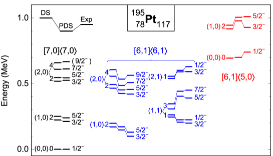
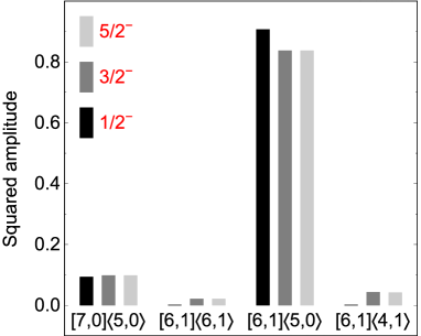
Figure 1: (Color online). Left panel: Observed and calculated energy spectrum of ¹⁹⁵Pt. The levels in black are the solvable $[7,0]\langle 7,0\rangle$ eigenstates of $\hat{H}_{\rm DS}$ (3), whose structure and energy remain unaffected by the added PDS interactions in Eq. (10). The levels in blue (red) are the $[6,1]\langle 6,1\rangle$ ($[6,1]\langle 5,0\rangle$) eigenstates of $\hat{H}_{\rm DS}$ (3) and are subsequently perturbed by the PDS interactions in Eq. (10). Right panel: ${\rm SO}^{\rm BF}(6)$ decomposition of the eigenstates of $\hat{H}_{\rm PDS}$ (10), shown in red on the left panel.

Table 2: Observed $B({\rm E}2;J_{\rm i}\rightarrow J_{\rm f})$ values between negative-parity states in ¹⁹⁵Pt compared with the DS and PDS predictions of the ${\rm SO}^{\rm BF}(6)$ limit. The solvable (mixed) states are members of the ground (excited) bands shown in Fig. 1. The E2 operator employed is defined in the text.

${E_{\rm i}}$		$J_{\rm i}$		${E_{\rm f}}$		$J_{\rm f}$		$B({\rm E}2;J_{\rm i}\rightarrow J_{\rm f}$) ($10^{-3}~{}e^{2}{\rm b}^{2}$)
(keV)				(keV)				Exp		DS		PDS
	Solvable $\rightarrow$ solvable
212		${3/2}$		0		${1/2}$		$190(10)$		179		179
239		${5/2}$		0		${1/2}$		$170(10)$		179		179
525		${3/2}$		0		${1/2}$		$17(1)$		0		0
525		${3/2}$		239		${5/2}$		$\leq 19$		72		72
544		${5/2}$		0		${1/2}$		$8(4)$		0		0
612		${7/2}$		212		${3/2}$		$170(70)$		215		215
667		${9/2}$		239		${5/2}$		$200(40)$		239		239
	Solvable $\rightarrow$ mixed
239		${5/2}$		99		${3/2}$		$60(20)$		0		0
525		${3/2}$		99		${3/2}$		$\leq 33$		7		3
525		${3/2}$		130		${5/2}$		$9(5)$		3		2
612		${7/2}$		99		${3/2}$		$5(3)$		9		11
667		${9/2}$		130		${5/2}$		$12(3)$		10		12
	Mixed $\rightarrow$ solvable
99		${3/2}$		0		${1/2}$		$38(6)$		35		34
130		${5/2}$		0		${1/2}$		$66(4)$		35		33
420		${3/2}$		0		${1/2}$		$15(1)$		0		0
456		${5/2}$		0		${1/2}$		$\leq 0.04$		0		0
508		${7/2}$		212		${3/2}$		$55(17)$		20		18
563		${9/2}$		239		${5/2}$		$91(22)$		22		22
199		${3/2}$		0		${1/2}$		$25(2)$		0		0
390		${5/2}$		0		${1/2}$		$7(1)$		0		0
	Mixed $\rightarrow$ mixed
420		${3/2}$		99		${3/2}$		$5(4)$		177		165
508		${7/2}$		99		${3/2}$		$240(50)$		228		263
563		${9/2}$		130		${5/2}$		$240(40)$		253		284
390		${5/2}$		99		${3/2}$		$200(70)$		219		179
390		${5/2}$		130		${5/2}$		$\leq 14$		55		35

The experimental spectrum of ¹⁹⁵Pt is shown in Fig. 1, compared with the DS and PDS calculations. The coefficients $c$, $d$, and $d^{\prime}$ in $\hat{H}_{\rm DS}$ (3) are adjusted to the excitation energies of the $[7,0]\langle 7,0\rangle$ levels which are reproduced with a root-mean-square (rms) deviation of 12 keV. The remaining two coefficients $a$ and $b$ are obtained from an overall fit. The resulting (DS) values are (in keV): $a=45.3$, $b=-41.5$, $c=49.1$, $d=1.7$, and $d^{\prime}=5.6$. The fit for the PDS calculation proceeds in stages. First, the parameters $c$, $d$, and $d^{\prime}$ in Eq. (3) are taken at their DS values. This ensures the same spectrum for the $[7,0]\langle 7,0\rangle$ levels (drawn in black in Fig. 1) which remain eigenstates of $\hat{H}_{\rm PDS}$ (10). Next, one considers the $[6,1]\langle 6,1\rangle$ levels and improves their description by adding the three PDS $U$ interactions. The resulting coefficients are (in keV): $a^{\prime}_{1}=10$, $a_{2}=-97$, and $a_{3}=112$. Eq. (5) ensures that the energies of the $[7,0]\langle 7,0\rangle$ levels do not change while the agreement for the $[6,1]\langle 6,1\rangle$ levels is improved (blue levels in Fig. 1). The rms deviation for both classes of levels is 20 keV. In particular, unlike in the DS calculation, it is possible to reproduce the observed inversion of the $1/2^{-}$-$3/2^{-}$ doublets without changing the order of other doublets. The additional PDS terms necessitate a readjustment of the $a$ coefficient in Eq. (3), for which the final (PDS) value is $a=37.7$ keV, while the coefficient $b$ is kept unchanged. Finally, the position of the $[6,1]\langle 5,0\rangle$ levels (red levels in Fig. 1) is corrected by considering the PDS $V$ interaction with $a_{0}=306$ keV which, due to Eq. (6), has a marginal effect on lower bands. The rms deviation for all levels shown in Fig. 1 is 23 keV. While the states $[7,0]\langle 7,0\rangle$ of the ground band are pure, other eigenstates of $\hat{H}_{\rm PDS}$ in excited bands can have substantial ${\rm SO}^{\rm BF}(6)$ mixing (see right panel of Fig. 1).

A large amount of information also exists on electromagnetic transition rates and spectroscopic strengths. In Table 2, 25 measured $B$(E2) values in ¹⁹⁵Pt are compared with the DS and PDS predictions. The same E2 operator is used as in previous studies Bruce85 ; Mauthofer86 of the ${\rm SO}^{\rm BF}(6)$ limit, $\hat{T}_{\mu}({\rm E2})=e_{\rm b}\hat{Q}^{\rm B}_{\mu}+e_{\rm f}\hat{Q}^{\rm F}_{\mu}$, where $\hat{Q}^{\rm B}_{\mu}=s^{\dagger}\tilde{d}_{\mu}+d^{\dagger}_{\mu}s$ is the boson quadrupole operator, $\hat{Q}^{\rm F}_{\mu}$ is its fermion analogue ibfm , and $e_{\rm b}$ and $e_{\rm f}$ are effective boson and fermion charges, with the values $e_{\rm b}=-e_{\rm f}=0.151$ $e$b. Table 2 is subdivided in four parts according to whether the initial and/or final state in the transition has a DS structure (as in Refs. Bruce85 ; Mauthofer86 ) or whether it is mixed by the PDS interaction. It is seen that when both have a DS structure the $B$(E2) value does not change, only slight differences occur when either the initial or the final state is mixed, and the biggest changes arise when both are mixed.

In summary, we have proposed a novel extension of the PDS notion to Bose-Fermi systems and exemplified it in ¹⁹⁵Pt. The analysis highlights the ability of a PDS to select and add to the Hamiltonian, in a controlled fashion, required symmetry-breaking terms, yet retain a good DS for a segment of the spectrum. These virtues greatly enhance the scope of applications of algebraic modeling of complex systems. The operators (8) with $\beta\neq 1$, can be used to explore additional PDSs in odd-mass nuclei. Partial supersymmetry, of relevance to nuclei Metz99 , can be studied by embedding the algebras of Eq. (1) in a graded Lie algebra. Work in these directions is in progress.

We thank Stefan Heinze for his help with the numerical calculations. J.J. acknowledges financial support by GANIL and by the Interuniversity Attraction Poles programme initiated by the Belgian Science Policy Officer under grant BrixNetwork P7/12 during a sabbatical stay at GANIL. A.L. acknowledges the hospitality of the Theoretical Division at LANL during a sabbatical stay, and the support by the Israel Science Foundation.

References

• (1) A. Bohm, Y. Néeman, and A. O. Barut Eds. Dynamical Groups and Spectrum Generating Algebras (World Scientific, Singapore, 1988).
• (2) F. Iachello and A. Arima, The Interacting Boson Model (Cambridge University Press, Cambridge, 1987).
• (3) F. Iachello and P. Van Isacker, The Interacting Boson–Fermion Model (Cambridge University Press, Cambridge, 1991).
• (4) K. Kikoin, M. Kiselev, and Y. Avishai, Dynamical Symmetries for Nanostructures (Springer-Verlag, Berlin, 2012).
• (5) F. Iachello and R. D. Levine, Algebraic Theory of Molecules (Oxford University Press, Oxford, 1994)
• (6) A. Frank and P. Van Isacker, Algebraic Methods in Molecular and Nuclear Physics, (Wiley, New York, 1994).
• (7) Y. Alhassid and A. Leviatan, J. Phys. A 25, L1265 (1992).
• (8) A. Leviatan, Phys. Rev. Lett. 77, 818 (1996).
• (9) A.G. Ushveridze, Quasi-Exactly Solvable Models in Quantum Mechanics (Taylor and Francis Group, New York 1994).
• (10) A. Leviatan, A. Novoselsky, and I. Talmi, Phys. Lett. B 172, 144 (1986).
• (11) P. Van Isacker, Phys. Rev. Lett. 83, 4269 (1999).
• (12) A. Leviatan and P. Van Isacker, Phys. Rev. Lett. 89, 222501 (2002).
• (13) A. Leviatan, Prog. Part. Nucl. Phys. 66, 93 (2011).
• (14) J. E. García-Ramos, A. Leviatan, and P. Van Isacker, Phys. Rev. Lett. 102, 112502 (2009).
• (15) A. Leviatan, J. E. García-Ramos, and P. Van Isacker, Phys. Rev. C 87, 021302(R) (2013).
• (16) R. F. Casten, R. B. Cakirli, K. Blaum, and A. Couture, Phys. Rev. Lett. 113, 112501 (2014); A. Couture, R. F. Casten, and R. B. Cakirli, Phys. Rev. C 91, 014312 (2015).
• (17) C. Kremer, J. Beller, A. Leviatan, N. Pietralla, G. Rainovski, R. Trippel, and P. Van Isacker, Phys. Rev. C 89, 041302(R) (2014).
• (18) J. L. Ping and J. Q. Chen, Ann. Phys. (N.Y.) 255, 75 (1997).
• (19) A. Leviatan, Phys. Rev. Lett. 98, 242502 (2007).
• (20) M. Macek and A. Leviatan, Ann. Phys. (N.Y.) 351, 302 (2014).
• (21) N. Whelan, Y. Alhassid, and A. Leviatan, Phys. Rev. Lett. 71, 2208 (1993); A. Leviatan and N. D. Whelan, Phys. Rev. Lett. 77, 5202 (1996).
• (22) J. Escher and A. Leviatan, Phys. Rev. Lett. 84, 1866 (2000); Phys. Rev. C 65, 054309 (2002).
• (23) D. J. Rowe and G. Rosensteel, Phys. Rev. Lett. 87, 172501 (2001); G. Rosensteel and D. J. Rowe, Phys. Rev. C 67, 014303 (2003).
• (24) P. Van Isacker and S. Heinze, Phys. Rev. Lett. 100, 052501 (2008); Ann. Phys. (N.Y.) 349, 73 (2014).
• (25) A. Arima and F. Iachello, Ann. Phys. (N.Y.) 123, 468 (1979).
• (26) J. A. Cizewski, R. F. Casten, G. J. Smith, M. L. Stelts, W. R. Kane, H. G. Börner, and W. F. Davidson, Phys. Rev. Lett. 40, 167 (1978).
• (27) P. Van Isacker, A. Frank, and H.-Z. Sun, Ann. Phys. (N.Y.) 157, 183 (1984).
• (28) R. Bijker and F. Iachello, Ann. Phys. (N.Y.) 161, 360 (1985).
• (29) B. G. Wybourne, Classical Groups for Physicists (Wiley, New York, 1974).
• (30) A. Metz, Y. Eisermann, A. Gollwitzer, R. Hertenberger, B. D. Valnion, G. Graw, and J. Jolie, Phys. Rev. C 61, 064313 (2000); Phys. Rev. C 67, 049901(E) (2003).
• (31) A. M. Bruce, W. Gelletly, J. Lukasiak, W. R. Phillips, and D. D. Warner, Phys. Lett. B 165, 43 (1985).
• (32) A. Mauthofer, K. Stelzer, J. Gerl, Th. W. Elze, Th. Happ, G. Eckert, T. Faestermann, A. Frank, and P. Van Isacker, Phys. Rev. C 34, 1958 (1986).
• (33) A. Metz, J. Jolie, G. Graw, R. Hertenberger, J. Gröger, C. Günther, N. Warr, and Y. Eisermann, Phys. Rev. Lett. 83, 1542 (1999).