Hierarchical structures in Northern Hemispheric extratropical winter ocean-atmosphere interactions
Abstract
In recent years extensive studies on the Earth’s climate system have been carried out by means of advanced complex network statistics. The great majority of these studies, however, have been focusing on investigating correlation structures within single climatic fields directly on or parallel to the Earth’s surface. Here, we develop a novel approach of node weighted coupled network measures to study correlations between ocean and atmosphere in the Northern Hemisphere extratropics and construct 18 coupled climate networks, each consisting of two subnetworks. In all cases, one subnetwork represents monthly sea-surface temperature (SST) anomalies, while the other is based on the monthly geopotential height (HGT) of isobaric surfaces at different pressure levels covering the troposphere as well as the lower stratosphere. The weighted cross-degree density proves to be consistent with the leading coupled pattern obtained from maximum covariance analysis. Network measures of higher order allow for a further analysis of the correlation structure between the two fields and consistently indicate that in the Northern Hemisphere extratropics the ocean is correlated with the atmosphere in a hierarchical fashion such that large areas of the ocean surface correlate with multiple statistically dissimilar regions in the atmosphere. Ultimately we show that, this observed hierarchy is linked to large-scale atmospheric variability patterns, such as the Pacific North American pattern, forcing the ocean on monthly time scales.
Keywords:
coupled climate networks, extratropical ocean-atmosphere interaction, node-weighted network measures, hierarchical networks
1 Introduction
In the last years, complex network analysis has been established as a powerful tool to study statistical interdependencies in the climate system [11, 55, 58, 57, 15]. Links in the so-called climate networks represent functional interdependencies indicated by significant correlations [12, 11, 41, 40] or the synchronous occurrence of extreme events [50, 5, 35, 36, 6] in climatic time series taken at different grid points or measurement sites on or parallel to the Earth’s surface.
In addition to studies on observational data of climate dynamics, climate networks have also been applied successfully to hindcast extreme events, such as extreme precipitation in South America [4], or to predict the occurrence of El Niño episodes [33, 34] and discriminate between different event types [66, 41, 56, 69].
So far, most studies conducted within the framework of climate networks focused solely on the dynamics within a single climatic field or layer. Besides atmospheric characteristics like surface air temperature, sea level pressure, or precipitation, recent studies have also addressed ocean dynamics represented by ocean temperature variability at the surface [19, 52] or different depths [37] as well as the spatio-temporal variability in the strength of the Atlantic meridional overturning circulation [20].
It is well known, however, that the dynamics within the two major subcomponents of the Earth’s climate system, ocean and atmosphere, are closely entangled [54, 22]. Examples for these interrelationships include the North Atlantic eddy-driven jet stream [67] or the Pacific ocean forcing to the atmosphere which is closely related to the dynamics of the El Niño Southern Oscillation [68]. Further, it has been shown that on time scales of up to one month the ocean is forced by atmospheric circulation, prominently manifested in terms of long-term variability patterns like the Pacific North American pattern [[, e.g.]]frankignoul_observed_2007 and the North Atlantic Oscillation [9, 23].
Inspired by approaches to investigate the interaction structure between different mutually coupled subsystems such as infrastructure networks [62, 8, 3] a novel set of coupled network measures has been proposed by [13] which provides a general tool to quantify interdependencies between subcomponents in complex coupled climate networks. The latter framework has been successfully applied to investigate interactions between different layers of geopotential height fields, where each isobaric surface forms a subcomponent of a larger climate network. Similarly, coupled climate networks have been constructed to study ocean-atmosphere interactions in the tropical Pacific [18] or over the South Atlantic Convergence Zone [53].
Following upon these previous studies, in this work we extend the approach by [13] and present an exploratory study to understand and quantify ocean-atmosphere interactions in the Northern Hemisphere mid-to-high latitudes during boreal winter at monthly scales. This temporal restriction is chosen, since previous studies by means of lagged maximum covariance analysis (MCA) have already revealed that the statistical interrelationship between atmosphere and ocean is strongest and most significant at lags of zero or one month during late fall and winter [[, e.g.]]czaja_influence_1999, wen_observations_2005, liu_observational_2006, frankignoul_observed_2007, gastineau_influence_2015.
To investigate further the spatial structure of these complex interaction patterns, we construct here in total 18 coupled climate networks consisting of two layers each, one layer representing sea surface temperature (SST) anomalies and the other geopotential height fields (HGT) at different pressure levels from 1000 to 10 mbar covering the entire troposphere as well as the lower stratosphere.
Our area of study covers the whole Northern Hemisphere north of N so that the density of grid points in the considered climate data sets increases rapidly towards the poles and induces some bias in the unweighted network measures [57, 41]. Therefore, the standard coupled network approach by [13] is not sufficient in the present case. To overcome the problem associated with the heterogeneous spatial density of grid points interpreted as nodes of the climate network, [28] introduced a novel set of network measures that takes into account the different sizes or weights of nodes in the network. By following an axiomatic approach, each standard (unweighted) network measure can be transformed into its weighted counterpart, the so-called node splitting invariant (n.s.i.) network measure. Corresponding n.s.i. measures have also been derived by [70] for edge-weighted and directed networks.
To quantify the topology of coupled climate networks, we rely in this work on the previously defined versions of local (i.e. node-wise) n.s.i. coupled network measures [18, 65] and additionally derive further weighted global network measures following the approach introduced by [28]. This allows us to assess and compare the macroscopic correlation structure in each of the 18 coupled climate networks.
We compare the results of MCA [[, e.g.]]storch_statistical_2001, a well-established standard tool from statistical climatology, with the cross-degree density of nodes in the different subnetworks and confirm expected similarities between the two measures [15]. By utilizing network measures of higher order such as the n.s.i. local cross-clustering coefficient, we find that the statistical interrelation between ocean and atmosphere exhibits a hierarchical structure, in which individual parts or areas of the ocean surface correlate strongly with multiple statistically dissimilar parts of the atmosphere. Building upon previous studies by, e.g., [21, 9], and [23] we relate the observed hierarchy to dominant atmospheric patterns forcing the ocean on the time scales investigated in this study.
The remainder of this paper is organized as follows. Section 2 introduces the data sets and all methods, i.e., maximum covariance analysis and coupled climate network analysis, that are applied in this study. Section 3 presents all results of the analysis followed by conclusions and an outlook discussing future research tasks in Section 4.
2 Data & Methods
2.1 Data description
We construct coupled climate networks from two different climatic observables in order to investigate their interaction structure. One subnetwork is based on monthly anomalies of geopotential height (HGT) fields obtained from the ERA40 reanalysis project of the European Centre for Medium-Range Weather Forecast [61]. The data is given on a regular latitude/longitude grid with a spatial resolution of . In total, we investigate layers of HGT fields. The corresponding pressure values at each isobaric surface as well as the average geopotential height are given in Tab. 1. The second subnetwork is constructed from the monthly averaged SST field (HadISST1) provided by the Met Office Hadley Centre [44] with a resolution of . All grid points with corresponding time series containing missing values are removed from the data set as they represent areas which have been at least temporarily covered by sea-ice.
For our analysis we investigate all grid points north of N excluding the North Pole itself. Both data sets are cropped in their temporal extent to cover the same time span from January 1958 to December 2001 and, hence, each time series consists of temporal sampling points. We obtain a total number of grid points for the SST data and grid points for each isobaric surface of HGT. For both data sets, we remove the annual cycle by subtracting the climatic mean for each month from each time series. Since we focus on the spatial structure of strong statistical interrelationships between ocean and atmosphere during boreal winter months (DJF), we use only the corresponding values which yields a length of each time series of data points.
2.2 Maximum covariance analysis (MCA)
Consider two sets of time series and representing two different climatic fields, which in the scope of our application are the SST field (in what follows indicated by the index s) and one layer i of HGT (see also Tab. 1). Further assume each individual time series in both fields to be normalized to zero mean and unit variance. The linear lag-zero cross-correlation matrix with entries is then defined as
| (1) |
where , and denotes the total number of temporal sampling points in the two time series. Due to the heterogeneous spatial distribution of grid points in the present data sets all matrix entries are additionally multiplied by the square roots of the cosine of latitudinal positions to ensure equal weighting. This then yields the weighted cross-correlation matrix with entries
| (2) |
Analogously to empirical orthogonal function (EOF) analysis [[, e.g.]]ghil_advanced_2002,hannachi_empirical_2007, MCA identifies orthonormal pairs of coupled patterns and for (with being the rank of ) which explain as much as possible of the covariance between pairs of time series taken from the two different climatic fields [[, e.g.]]bretherton_intercomparison_1992,storch_statistical_2001. The coupled patterns are obtained by solving the singular value problem of the weighted cross-covariance matrix,
| (3) | ||||
| (4) |
They are ordered according to their respective singular values with . Hence, denotes the largest among the singular values that can be found to solve the above equations. Therefore, and are referred to as the leading coupled patterns representing the largest fraction of squared covariance between the two climatic fields given by .
2.3 Coupled climate network construction
In climate networks, each node represents a climatic time series and links indicate strong correlations between two series. Hence, the () correlation matrix contains the pairwise linear statistical relationships between all time series considered for the network construction. Here, we independently construct coupled climate networks for all combinations of the SST field and each of the 18 isobaric surfaces of HGT, which shall be investigated separately and rely on the linear Pearson correlation coefficient as an appropriate measure of statistical association. Hence, the correlation matrix has the form
| (5) |
The two block matrices () and () represent the (internal) correlation matrices of the SST and HGT fields, respectively, which consist of elements
| (6) | ||||
| (7) |
The elements of are derived according to Eq. (1). Note, that (in contrast to the computation of the leading coupled patterns) we construct the coupled climate networks from the unweighted correlation matrix C, while the correction for the heterogeneous spatial distribution of nodes is implemented into the corresponding network measures (see Sec. 2.4).
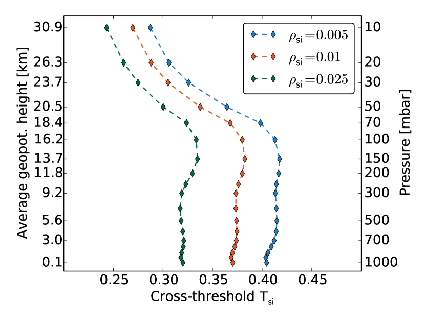
From the correlation matrix C one generally derives the network’s adjacency matrix by setting a fixed threshold such that only a certain fraction (i.e. the link density ) of strongest correlations is represented by links in the resulting climate network. For obtaining the adjacency matrix of coupled climate networks, we refine this procedure by fixing a desired link density for the structure of internal links within the two subnetworks representing SST and HGT fields, respectively. This means that only nodes with a correlation above the empirical 99th percentile of correlations between all time series within each field are connected. This condition then leads to internal correlation thresholds for the SST field and for each isobaric surface of HGT (Tab. 1). Usually, the dynamics within the different climatic fields shows much higher cross-correlations than between them. We account for this fact by assuming the fraction of significant interactions between the climatic fields to be lower than those within them. Specifically, we request a cross-link density of , which is lower than the internal ones, and derive a cross-threshold for each layer of HGT individually (Fig. 1). All internal thresholds and are significantly larger than the obtained cross-thresholds . Thus, setting a global link density or threshold would cause no or few cross-links to be present between the two fields or respective subnetworks. We further note that all links in each of the coupled climate networks represent correlations that are significant at least at the 95% confidence level of a standard t-test, where the degrees of freedom are determined by the total number of temporal sampling points in each of the time series (with we thus obtain 130 degrees of freedom when neglecting the presence of serial correlations in the individual time series).
The different values of already give an impression of the strength of correlation between the SST field and the different isobaric layers: low thresholds generally indicate weaker correlations while high thresholds imply stronger similarity between both fields. Further we note that the resulting cross-thresholds vary smoothly with the choice of cross-link density (Fig. 1) and we thus consider the construction mechanism to be sufficiently insensitive to the actual choice of cross-link density.
Using the different thresholds introduced above, we obtain the coupled climate network’s adjacency matrix by individually thresholding the absolute correlation values between and within both fields as
where denotes the Heaviside function. Note that in most recent studies on climate networks self-loops (resulting in a non-vanishing trace of the adjacency matrix) have been excluded. In this case the adjacency matrix is usually denoted as A. Since we aim to apply node splitting invariant network measures (see below) to quantify the network’s topology we specifically demand each node to be connected with itself. The resulting matrix is referred to as the extended adjacency matrix [28]. Further note, that the usage of the term coupled in coupled climate networks does not imply the notion of any directionality or causal influence between the two fields under study. It is simply meant to indicate the fact that the network under study is composed of more than a single climatic field.
2.4 Coupled network characteristics
The local (point-wise) and global structure of a climate network can be quantified by a variety of network measures [39, 1, 11], which can generally be interpreted as specific operations on the adjacency matrix. The climate networks in this study are constructed from climate data sets where the density of grid points and, hence, the density of nodes in the network, rapidly increases towards the North pole. In order to avoid a bias in the evaluation of the climate network’s structure, we account for this effect by relying on node-weighted network measures and value nodes with a gradually decreasing weight as one moves from the equator towards the pole. To quantify the correlation structure between ocean and atmosphere at each node we focus on two previously defined node weighted local network measures, the n.s.i cross-degree [18] and the n.s.i. local cross-clustering coefficient [65]. In addition, we utilize the construction mechanism introduced by [28] to convert global interacting network measures [13] into their weighted counterparts.
2.4.1 Preliminaries
Consider a coupled climate network with a set of nodes , links and the number of nodes . Following the general naming convention in the climate network framework we identify every node with a natural number , such that serves as the label of the node as well as an index to corresponding network characteristics. The network is represented by its adjacency matrix A with . In this study, each coupled climate network is composed of two subnetworks, representing the ocean and representing a specific atmospheric layer. The set of nodes divides into subsets and such that each node belongs to exactly one subnetwork (i.e. and ). Likewise, the set of links splits into internal link sets and (connecting nodes within a subnetwork) and cross-link sets connecting nodes with nodes in the subnetworks and , respectively [13].
In the present case (as for all regularly gridded climate data sets) the share on the entire area of the surface that is represented by each node is governed by its latitudinal position on the grid. Following [57], we therefore assign to each node in the climate network a weight
| (8) |
Note that, by following this convention the climate networks’ node weights exhibit the same dimension as the weights of the cross-covariance matrix in Eq. (2).
[28] introduced a novel set of node splitting invariant (n.s.i.) network measures to quantify the topology of a climate network with such a heterogeneous spatial node density for the case of a single-layer network and, hence, only one climate variable under study. In fact, the n.s.i. network measures are not restricted to climate networks but can be utilized to study any type of single-layer complex network where nodes represent entities of different weights. [28] further showed that each complex network measure can be transformed into its weighted counterpart by using a four-step construction mechanism:
-
(a)
Sum up weights whenever the unweighted measure counts nodes.
-
(b)
Treat every node as connected with itself.
-
(c)
Allow equality in summations over indices and wherever the original measure involves a sum over distinct nodes and .
-
(d)
“Plug in” n.s.i. versions of measures wherever they are used in the definition of other measures.
From the definition of the adjacency matrix in Eq. (2.3) we note that step (b) of the above scheme is in our case already fulfilled. [65] and [70] recently utilized the proposed scheme to convert local interacting network measures as well as measures for directed networks into their weighted counterparts. Here, we additionally derive n.s.i. versions of some global cross-network measures that were introduced by [13].
2.4.2 Local measures
For quantifying local cross-network interactions in coupled climate networks we rely on two measures, n.s.i. cross-degree and n.s.i. local cross-clustering coefficient , that were introduced by [65] and (for the case of the n.s.i. cross-degree) by [18]. These two measures are defined as
| (9) | ||||
| (10) |
In contrast to the unweighted cross-degree
| (11) |
which simply counts nodes that are connected with , is proportional to the share on the considered overall ice-free ocean or isobaric surface area, respectively, that is connected with nodes in the other subnetwork. It therefore gives a notion of how similar the dynamics at a node is to that of the other climate variable observed at all available grid points.
Similar to , no longer relies on the counting of distinct fully connected node triples in the network (as for the classical local clustering coefficient [39]) but on the weighted sum of occurrences of triples of connected areas within the two subnetworks. It gives the probability that an area represented by a node is connected with two mutually connected and, hence, dynamically similar, areas in the opposite subnetwork. In this spirit, estimates how likely areas in two different climatic fields or subsystems form clusters of statistical equivalence between them. A local accumulation of such connected triples represents clusters of closely connected nodes and, in the spirit of climate networks, strongly correlated regions.
In order to make the n.s.i. cross-degree comparable between the two subnetworks, we normalize it by the maximum possible weight that nodes can be connected with,
| (12) |
In the spirit of earlier work by [14] and [17], we refer to this quantity as the n.s.i. cross-degree density. Here, denotes the total weight of all nodes . For the case of a single-layer network, a measure similar to the n.s.i. cross-degree density has been introduced by [57] in terms of the area weighted connectivity, which quantities the share on the subdomain of interest represented by the entire network that is connected with any nodes .
Generally, [65] and [70] showed that the weighted local cross-network measures improve the representation of a network’s topology with inhomogeneous node density within the domain of interest in comparison with its unweighted counterparts.
[15] showed that for the unweighted case cross-degree and leading coupled patterns display strong similarity if the first coupled patterns explain a high fraction of the system’s covariance. A similar assessment can be made for the similarity between the leading coupled patterns obtained from a weighted cross-covariance matrix and the n.s.i. cross-degree (see supporting information).
2.4.3 Global measures
In addition to local (per node) network measures we also aim to characterize the macroscopic interaction structure of each pair of coupled climate networks by means of global network properties. For coupled climate networks a variety of unweighted measures have been proposed by [13]. Here, we utilize the construction mechanism by [28] to convert two of them into their weighted counterparts as well.
N.s.i. global cross-clustering coefficient.
The global cross-clustering coefficient of a subnetwork gives the probability that for a randomly chosen node one finds neighbors that are mutually linked. It is defined as the arithmetic mean of all local cross-clustering coefficients ,
| (13) |
This measure can be converted into its n.s.i. counterpart by calculating the weighted mean of all values of ,
| (14) |
Again, analogously to the interpretation of the local n.s.i. measures, no longer only measures pure node-wise triangular structures but takes into account the share on the Earth’s surface areas involved in the formation of triangular structures. Generally, large values of (which are induced by a dominance of connected triples between the two subnetworks under consideration) indicate strong transitivity in the underlying correlation structure.
N.s.i. cross-transitivity.
The cross-transitivity gives the probability that two randomly drawn nodes are connected if they have a common neighbor . It is given as
| (15) |
Like , the cross-transitivity is a measure of organization with respect to the cross-correlation structure in a coupled network [13]. However, in contrast to , takes into account the increasing influence of nodes with high cross-degree and weighs them more heavily than nodes with low cross-degree. More importantly it ignores nodes with no links into the opposite layer, since these nodes display a zero cross-degree. The node-weighted variant of can be written as
| (16) |
We note that both and similarly evaluate the transitivity of correlations between the two climatic variables under study and, hence, quantify a similar network property. They are derived, however, in a disjoint manner. One measure, is computed as the weighted average taken over . In contrast, despite suggestions by [41] to decompose the global transitivity into local contributions, the n.s.i. cross-transitivity is defined solely as a global network measure with no direct local counterpart. It is important to note that n.s.i. cross-transitivity and n.s.i. global cross-clustering coefficient are commonly asymmetric in the sense that and .
3 Results
3.1 Maximum covariance analysis (MCA)
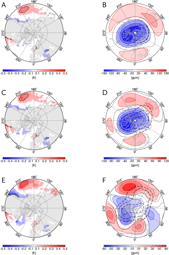
We start our analysis by computing the leading coupled patterns between the SST field and the 18 HGT layers for boreal winter (DJF). Figure 2 displays the results for three representative layers of HGT at 50 mbar, 100 mbar and 500 mbar.
By applying MCA, we detect coherent large-scale patterns of winter SST, which co-vary with the winter atmospheric circulation structures instantaneously. The leading MCA patterns explain rather large amounts of 42%, 63% and 70% (for the 500, 100 and 50 mbar pressure level, respectively) of the squared covariance. At all levels, the leading MCA mode displays significant SST anomalies over the North Pacific with maximum values along the sub-Arctic front near 40∘N, and anomalies of the opposite sign along the western coast of North America (Fig. 2A,C,E) [21, 2]. Over the North Atlantic, a dipole structure is seen between the northern part of the Gulf Stream and the Atlantic Ocean south of Greenland including parts of the Davis Strait and the North Atlantic current. This pattern resembles the first SST EOF for the Northern Hemisphere during boreal winter (not shown).
This general SST pattern is co-varying with a pressure anomaly pattern showing a hemispheric annular-like structure in the upper troposphere and lower stratosphere (Fig. 2B,D). In the mid-troposphere (Fig. 2F), this pattern displays wave-like deviations from the annular structure, which show distinct similarities with the wave-train structure of the Pacific North American (PNA) pattern. Therefore, the leading MCA mode relates negative SST anomalies along the sub-Arctic front with a positive PNA phase.
The second MCA mode (not shown, explaining 13%, 17% and 21% of the squared covariance fraction for the 500, 100 and 50 mbar pressure level, respectively) displays the strongest SST anomalies over the North Atlantic. Over that region, the SST pattern resembles the northern part of the North Atlantic SST tripole pattern which is related with the North Atlantic Oscillation (NAO) [[, e.g.]]czaja_influence_1999, czaja_observed_2002, gastineau_influence_2015. Accordingly, the co-varying atmospheric pattern in the middle troposphere shows the cold ocean/warm land (COWL) pattern (introduced by [63]) including a NAO-like dipole over the North Atlantic. At higher levels, the co-varying atmospheric patterns display a pronounced wave number-2 pattern.
By applying lagged MCA between SST and mid-tropospheric circulation fields, several studies for the North Atlantic and the North Pacific have shown that the squared covariance fraction is strongest and most significant at lags of 0 and 1 month during late fall and winter [[, e.g.]]czaja_influence_1999, wen_observations_2005, liu_observational_2006, frankignoul_observed_2007, gastineau_influence_2015. This points to the forcing of the SST by the dominant atmospheric pattern, which is the PNA pattern over the Pacific-North American sector [[, e.g.]]frankignoul_observed_2007 and the North Atlantic Oscillation (NAO) over the North Atlantic-European region [9, 23]. On the other hand, results of lagged MCA analyses with the ocean leading by 1 to 4 months in [21] and [23] suggest that the SST anomalies have a substantial influence on the large-scale atmospheric circulation at these time-scales.
3.2 Local coupled network measures
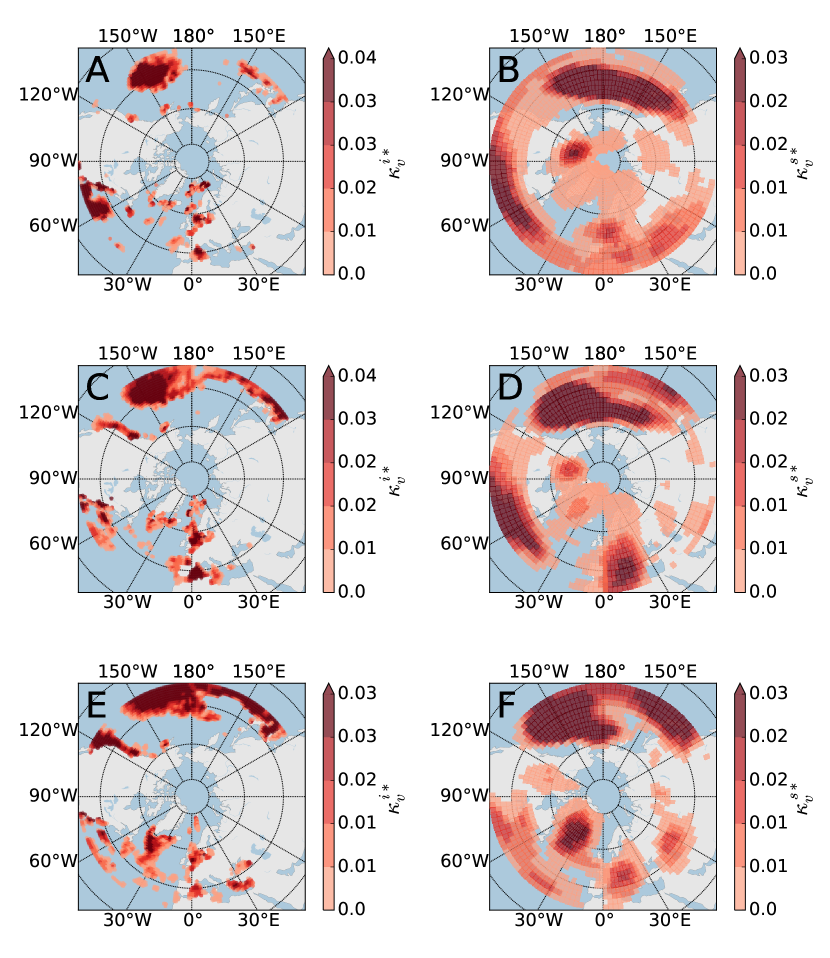
In order to first demonstrate the general consistency of coupled climate network analysis in comparison with MCA, we continue by generating coupled climate networks between the SST field and the three previously considered layers of geopotential height (500 mbar, 100 mbar, 50 mbar). The n.s.i. cross-degree densities and are expected to display similar spatial structures as the corresponding leading coupled patterns [15] since the latter explain a high share of the cross-covariance between both fields (see supporting information).
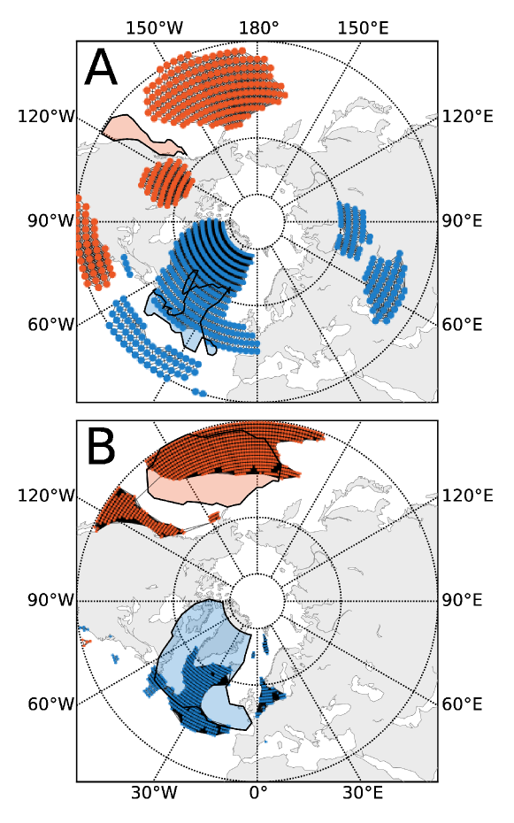
As demonstrated in Fig. 3, the results for and indeed match well the results obtained from the MCA when comparing the locations of maximum values in the coupled network’s n.s.i. cross-degree densities to those of maximum or minimum values in the leading mode of the MCA. Note, that the n.s.i. cross-degree densities and take, per definition, only positive values, while coupled patterns display both, positive and negative values. Hence, and only reproduce structures that coincide with the absolute values of the leading coupled patterns. However, as only a certain percentage of squared covariance is explained by the leading coupled patterns, we also note differences between the patterns revealed by the two methods. In particular, the negative center of action around the North Pole that is detected by MCA is only weakly present in the cross-degree density fields for the 50 and 100 mbar HGT fields (compare Fig. 2B,D with Fig. 3B,D). For the ocean, preferably the marked structures in the leading coupled patterns in both the Atlantic and the Pacific are well recovered by the cross-degree density while some of the weaker structures, e.g. in the Black Sea, are missing.
Network analysis, however, allows us to undertake a further in-depth analysis of the correlation structure between the different layers beyond the information provided by MCA. The n.s.i. local cross-clustering coefficients and (Eq. (10)) give the probabilities that the dynamics at a grid point in, e.g., the SST field is similar to that at two grid points in the HGT field, which behave themselves statistically similar. Note that in the scope of this work we do not account for any possible effects induced by a common external forcing of the fields, which might artificially induce correlations and, hence, cause the presence of spurious links between nodes or triples of nodes. We also do not account for indirect (partial) correlations or common driver effects within each of the fields when constructing the coupled climate networks. Conditioning out these possible influences by means of information theoretic approaches [45, 46] and causal effect networks [30, 47] thus remains as a subject of future research.
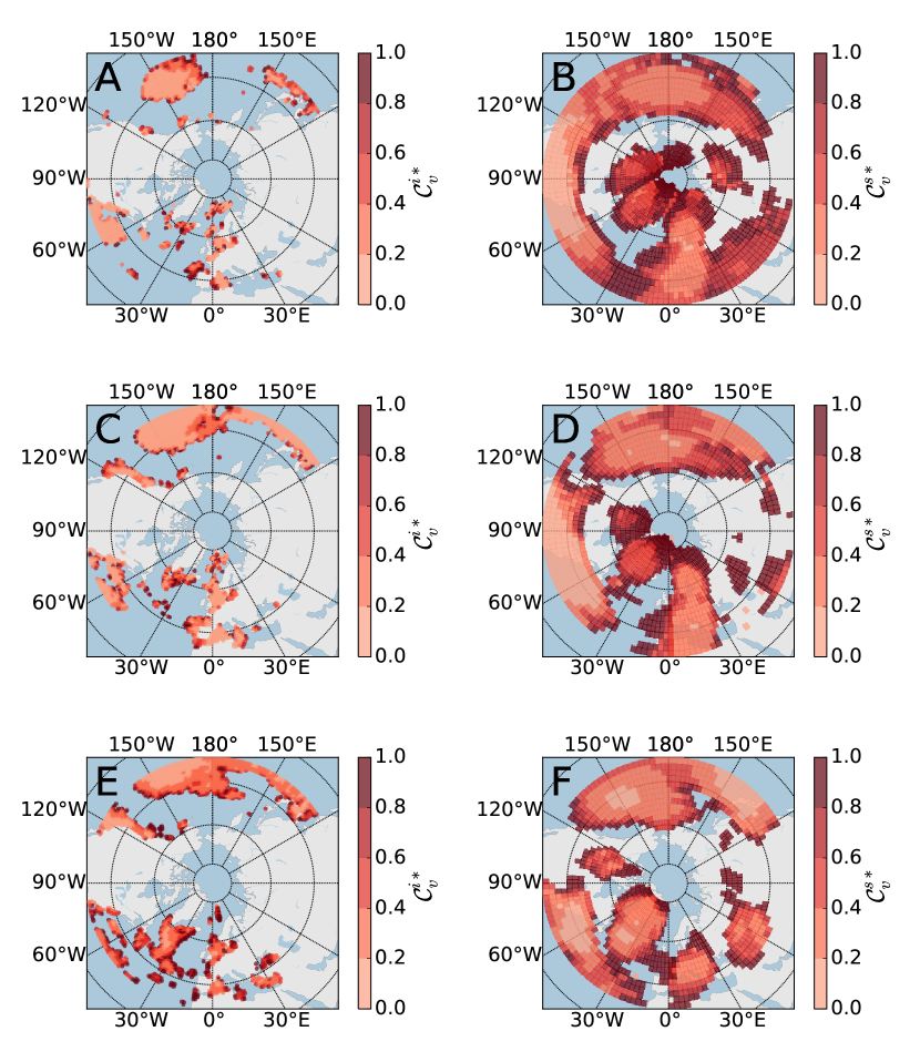
Figure 4 presents the results for the n.s.i. local cross-clustering coefficients for nodes in the SST field (Fig. 4A,C,E) and for nodes in the HGT fields (Fig. 4B,D,F). Most nodes in the SST field tend to display a low n.s.i. local cross-clustering coefficient (Fig. 4A,C,E) and, thus, preferentially correlate with nodes in the HGT fields that are mutually dissimilar and therefore disconnected (Fig. 5). In contrast, many nodes in the HGT fields exhibit a comparatively high or intermediate n.s.i. local cross-clustering coefficient (for one of the most prominent examples compare nodes located at or above the Pacific in Fig, 4B,D). Quantitatively, for the combination of the SST and the 500 mbar HGT field we find an n.s.i. global cross-clustering coefficient (Eq. (14)) of for SST nodes and for 500 mbar HGT nodes. Ignoring those nodes in the averaging that display zero n.s.i. cross-degree density we obtain values of and (note that this definition is different from the one presented in Eq. (14) as we specifically exclude the contribution of nodes with no links to the opposite subnetwork). The n.s.i. cross-transitivity (Eq. (16)) which weighs nodes according to their n.s.i. cross-degree density gives values of and for nodes in ocean and atmosphere, respectively. For all three measures, the values computed for the atmospheric subnetwork exceed those for the ocean and thus consistently imply that nodes in the ocean are less likely to connect with mutually connected nodes in the atmosphere than vice versa.
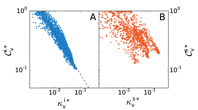
To further quantify the asymmetries in the correlation structure between ocean and atmosphere, we investigate for each node with a given n.s.i. cross-degree density its corresponding n.s.i. local cross-clustering coefficient in a coupled climate network composed of the SST and 500 mbar HGT fields (Fig. 6). This layer is chosen as it provides a good indication of the atmospheric circulation over the area of study [23, 31]. Furthermore, it displays among the highest values of according to Fig. 1, which has similarly been described as a strong statistical signal by [21].
For nodes in the SST field (Fig. 6A), we find that tends to follow a power-law, , which indicates a hierarchical network structure [43, 42] which, in contrast, is absent for nodes in the HGT field (Fig. 6B). Here, the term hierarchical implies that nodes in the SST field strongly correlate with disconnected clusters of statistically similar nodes in the HGT field as depicted in Fig. 5. This deduction is further supported by the fact that for the HGT field, the distribution of combinations of and is more widely spread and generally takes higher values than . This implies that nodes in the HGT field show a stronger tendency to correlate with mutually connected nodes in the SST field, which can be assumed to display a strong statistical similarity among themselves [38, 60]. To test for the robustness of our results we have carried out the same analysis as presented in Fig. 6 for internal link densities of and , and corresponding cross-link densities and (see Figs. 1 and 2 in the supporting information). Even though the power-law exponent slightly decreases towards zero with increasing link densities, we find that the qualitative findings remain unchanged. We thus consider our analysis to be sufficiently robust with respect to the actual choice of link densities.
As a remark, we note a general tendency of nodes at the boundaries of a cluster that links with the opposite field to display comparatively low values of n.s.i. cross-degree density and increased values of n.s.i. local cross-clustering coefficient (Fig. 3 and Fig. 4). In contrast, nodes located towards the center of these clusters display increased n.s.i. cross-degree density, which is in general to be expected from the continuity of the underlying system. However, in that case we also note tendencies for decreased values of n.s.i. local cross-clustering coefficients. This observation is a result of the fact that especially those nodes with only one link to the opposite field show by definition the highest value of the n.s.i. local cross-clustering coefficient, . With increasing n.s.i. cross-degree density this measure converges to a more reasonable estimate of a node’s tendency to cluster.
One way to address this issue in the future would be to subtract the squared sum of weights of all neighbors of the considered node from the numerator in Eq. (10). Such procedure would, however, introduce a non-standard network measure whose properties should be assessed thoroughly in future research before applying it to climatic studies. To this end, we acknowledge that the concerned nodes do not play a crucial role for the propositions put forward in this section, since they (i) are ultimately dealt with by the assessment of n.s.i. cross-transitivity which weighs those corresponding nodes much lower than those with a high n.s.i. cross-degree density and (ii) only manifest in the very upper left corners of Fig. 6A,B. In that case they do not contribute significantly to the observed relationship between n.s.i. cross-degree density and n.s.i. local cross-clustering coefficient and have no further impact on the qualitative statements put forward above.
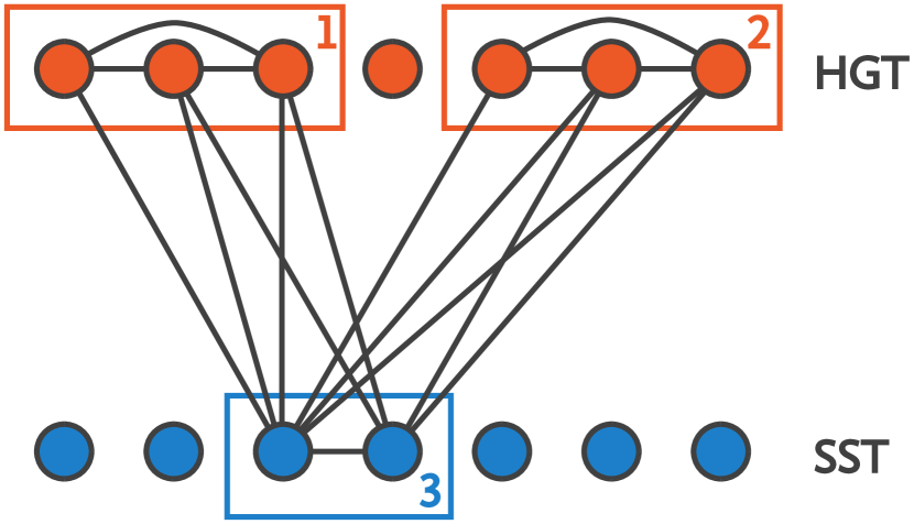
Following upon the quantitatively observed hierarchy, Fig. 7 allows for a visual inspection of some illustrative parts of the corresponding network structure. In particular, we display for two selected patches of nodes in the SST field that show high values of with the HGT field (blue and orange shaded polygons in Fig. 7A) their corresponding neighboring nodes in the HGT field as well as all links between those nodes (respective blue and orange scatter in Fig. 7A). While ignoring very small clusters we find in total four (three) substantial mutually disconnected patches of nodes in the HGT field that correlate with the respective ocean patches. Vice versa, by selecting the resulting two largest patches of nodes in the HGT field above both oceans (blue and orange shaded polygons in Fig. 7B) we find that each of the patches only correlates with two disconnected patches of nodes in the SST field that are of a relevant spatial extent to have an effect on the estimation of . Thus, the resulting n.s.i. cross-clustering coefficient for nodes in the ocean exceed for nodes in the atmosphere as the ocean correlates with more mutually disconnected clusters of nodes than vice versa.
Comparing the observed node patches in the HGT field with atmospheric patterns of large-scale variability patterns [25], we relate the two atmospheric clusters in the HGT field that are located above the Atlantic (blue scatter in Fig. 7A) with the NAO. Correspondingly, the three patches located above the Pacific (orange scatter in Fig. 7A) coincide well with the spatial signature of the PNA pattern. Taking into account past studies that applied lagged correlation analysis we note that on the time scales considered in this study the atmosphere serves as a driving force of the ocean along the spatial domain that is of interest here [[, e.g.]]frankignoul_observed_2007,czaja_influence_1999, gastineau_influence_2015. Thus, the hierarchical network structure might on the one hand be a result of the aforementioned atmospheric forcing to the ocean. On the other hand, with reference to Fig. 7, the framework of coupled climate networks and the methodology put forward in this work serve to resolve the corresponding induced correlation structure between the two climatic subsystems in a spatially explicit way, such that it enables to specifically detect forcing and forced areas in atmosphere and ocean, respectively.
Choosing different HGT layers up to 200 mbar yield similar results (not shown). This aligns well with previous results by [9] and [21] who observed comparable spatial statistical patterns at each tropospheric level. Thus, the observed hierarchy seems to be a generic property of the troposphere. Following the above lines of thought, future work should investigate coupled climate networks constructed from lagged cross-correlations to investigate whether the observed structures are indeed a result of short-term atmosphere-to-ocean forcing. Such procedure would, however, require the derivation of novel directed interacting network measures, which in turn would provide a valuable extension to the framework of climate network analysis.
3.3 Global measures
So far we have focused our study on three atmospheric layers, namely the 50 mbar, 100 mbar and 500 mbar HGT field. Specifically for the latter case, we have carried out a further in-depth analysis of the observed hierarchical structures by means of assessing the power-law relationship between and as well as investigating the distinct spatial distribution of nodes and links in ocean and atmosphere that obey the observed hierarchical organization (Fig. 7). To show that these structures are (i) not only present for the 500 mbar field and (ii) their observations are robust with respect to the choice of link densities we investigate global network characteristics that provide a macroscopic description of the observed network structures.
Specifically, we study the n.s.i. cross-transitivity computed over nodes in the SST field and computed over nodes in each of the HGT fields according to Eq. (16) together with the n.s.i. global cross-clustering coefficients and , respectively (Eq. (14)). Note again that the latter are defined as the weighted means of their local counterparts that are presented in Fig. 4, where nodes with no links to the opposite field are weighted in the same fashion as those with adjacent cross-links. In contrast, the n.s.i. cross-transitivity assigns nodes a weight corresponding to their n.s.i. cross-degree (which for the case of no adjacent cross-links takes a value of zero) and, thus, excludes them from the averaging.
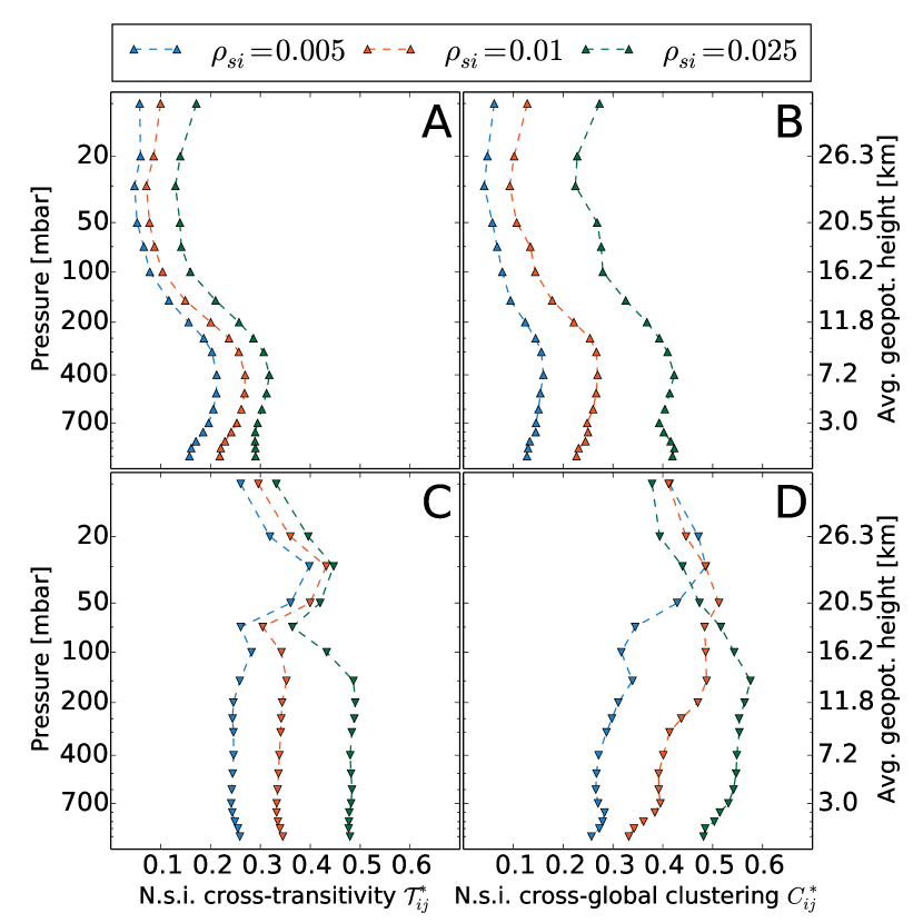
The corresponding results are summarized in Fig. 8. We find that both and show their maximum values at around 10 km altitude (250 mbar) (Figs. 8A and 8B). For the same quantities, distinct minima at 850 mbar (1.4 km) coincide with the transition from the atmospheric boundary layer to the lower troposphere as also found in [13]. For all layers above 100 mbar, remains almost constant at low values. Hence, and seem to naturally discriminate between three different atmospheric layers: below 850 mbar (atmospheric boundary layer), between 850 mbar and 100 mbar (free troposphere) and above 100 mbar (lower stratosphere).
For the global measures computed over all nodes in the HGT field, we find that the n.s.i. cross-transitivity shows almost constant values for all layers below 200 mbar and, hence, again separates well the dynamics within the troposphere from that inside the stratosphere (Fig. 8C). For all layers above 200 mbar becomes almost independent of the cross-link density that is fixed when constructing the network. The same property also holds for the n.s.i. global cross-clustering coefficient computed over all nodes in the different HGT fields (Fig. 8D).
In agreement with the local measures discussed in Sec. 3.2 we find that n.s.i. cross-transitivity and n.s.i. global cross-clustering coefficients are in most cases larger for nodes in the HGT fields than for nodes in the SST field (compare Fig. 8A with Fig. 8C and Fig. 8B with Fig. 8D). As for the n.s.i. local cross-clustering coefficients this indicates again the hierarchical network structure, i.e., a tendency for nodes in the HGT field to form triangular structures with nodes in the SST field, that is present across all atmospheric layers ranging from the troposphere to the lower stratosphere. The detailed structure of this hierarchy, however, seems to vary with the different atmospheric layers under study.
This observation further holds not only for the case of that was used in the previous sections but also for larger values that are chosen from a reasonable range (Fig. 8). Thus, we consider our results to be sufficiently robust with respect to the choice of the networks’ link densities.
In general, we observe that the quantitative and qualitative properties of the n.s.i. cross-transitivity and n.s.i. global cross-clustering coefficients vary with the different atmospheric layers. Hence, these global characteristics may serve to inter-compare and distinguish between different correlation structures in a coupled climate network. An in-depth analysis of the mechanisms that cause the occurrence of this behavior in our specific application remains as a subject of future research.
4 Conclusions & Outlook
We have carried out a detailed analysis of the correlation structure between atmospheric and ocean dynamics in the Northern Hemisphere extratropics from the viewpoint of coupled climate networks. Comparison between the n.s.i. cross-degree density (measuring the weighted share of significant correlations between grid points in different layers) and the leading mode of the maximum covariance analysis (MCA) reveals an expected high congruence between both methods for the considered data sets. However, coupled network analysis, and particularly the investigation of higher-order network parameters, allows us to further disentangle the underlying correlation structure. The (average) n.s.i. cross-degree density in combination with the (average) n.s.i. local cross-clustering coefficient provides additional insights on areas in the ocean and the atmosphere that show strong mutual correlations as well as localized versus delocalized correlation structures with the respective opposite field. In the SST field nodes tend to correlate with multiple mutually unconnected groups of similar nodes within the respective HGT fields. From investigating the interdependency between n.s.i. cross-degree density and n.s.i. local cross-clustering coefficient, we have found that the correlations between the ocean and the atmosphere exhibit a hierarchical structure in the sense of a power-law relationship between both properties. A visual inspection of the coupled climate network for the case of the 500 mbar HGT field reveals that the observed structure could be related with a forcing of the ocean by the dominant atmospheric patterns above the Atlantic and the Pacific. Ultimately, global network characteristics further support the results obtained from their local correspondents by showing that the observed structure is valid for large parts of the atmosphere ranging from the troposphere to the lower stratosphere.
In order to discriminate between the internal variability of the fields under study and possible influences of an external forcing, future work should analyze ensemble simulations of general circulation models to rule out common driver effects or assess the likelihood of their influence on the observed structures. In order to investigate the influence of spatio-temporal auto-correlation on the outcome of the present analysis the network could be alternatively constructed by estimating pairwise thresholds from surrogate data as proposed by [40]. This approach would, however, break the comparability of the network approach with that of maximum covariance analysis, such that a different way of validating and comparing the results must be found. Comparability could be achieved by assessing synthetic model data, e.g., created from an auto-regressive process based on principal components of the data sets under study, and the application of both, MCA and network analysis. In addition to probable influences of auto-correlation such a process would allow to assess the influence of different time scales in ocean and atmosphere on the involved network characteristics.
Besides all possible future lines of work with respect to the climatic side of this work, from a network-theoretic point of view it is worthwhile to construct climate networks using more advanced causal estimators [[, e.g.]]runge_quantifying_2012,runge_quantifying_2013,runge_identifying_2015 to disentangle direct from indirect or externally and internally forced correlations.
To this end, our analysis has only been performed for the pairwise correlation between one atmospheric layer and the ocean. Future studies should further explore the possibility to refine the proposed methods to also quantify interactions in a climate network existing of more than two subnetworks. Specifically, when studying coupled climate networks in the Northern Hemisphere, one should also consider Arctic sea ice as an additional observable in the network construction. Its dynamics has already been discovered as an influencing factor on atmospheric teleconnections and the dynamics of land snow cover in the Northern Hemisphere [26]. The study of coupled climate networks can help here to further disentangle and quantify possible changes in correlations between ocean and atmosphere over the course of the past decades that may have been induced by processes related to the Arctic amplification [48]. Moreover, it is of great interest to apply our methods not only to coupled networks composed of different climatic fields (as presented in this work), but also to networks constructed from just one single climatic field that divides into dynamically distinct areas [29] or communities [59, 49]. The framework presented in this work could then be utilized to study and quantify correlations between these detected or defined regions on or parallel to the Earth’s surface. This would allow for a detailed investigation of correlation structures between different climatic subsystems such as, for example, the Indian Summer Monsoon and the El Niño Southern Oscillation.
Finally, it remains to remark that the weighted network measures presented in this work provide a general framework which can be applied to quantify interdependencies in complex networks representing subjects of study taken from many other fields beyond climatology.
Acknowledgements
MW and RVD have been supported by the German Federal Ministry for Education and Research via the BMBF Young Investigators Group CoSy-CC2 (grant no. 01LN1306A) and the Belmont Forum/JPI Climate project GOTHAM. JFD is grateful for financial support by the Stordalen Foundation (via the Planetary Boundary Research Network PB.net) and the Earth League’s EarthDoc program. JK acknowledges the IRTG 1740 funded by DFG and FAPESP. Coupled climate network analysis has been performed using the Python package pyunicorn [16] that is available at https://github.com/pik-copan/pyunicorn.
References
- [1] Réka Albert and Albert-László Barabási “Statistical mechanics of complex networks” In Reviews of Modern Physics 74.1, 2002, pp. 47–97 DOI: 10.1103/RevModPhys.74.47
- [2] Soon-Il An and Bin Wang “The Forced and Intrinsic Low-Frequency Modes in the North Pacific” In Journal of Climate 18.6, 2005, pp. 876–885 DOI: 10.1175/JCLI-3298.1
- [3] S. Boccaletti, G. Bianconi, R. Criado, C. I. Genio, J. Gómez-Gardeñes, M. Romance, I. Sendiña-Nadal, Z. Wang and M. Zanin “The structure and dynamics of multilayer networks” In Physics Reports 544.1, 2014, pp. 1–122 DOI: 10.1016/j.physrep.2014.07.001
- [4] N. Boers, B. Bookhagen, H. M. J. Barbosa, N. Marwan, J. Kurths and J. A. Marengo “Prediction of extreme floods in the eastern Central Andes based on a complex networks approach” In Nature Communications 5.5199, 2014 DOI: 10.1038/ncomms6199
- [5] Niklas Boers, Bodo Bookhagen, Norbert Marwan, Jürgen Kurths and José Marengo “Complex networks identify spatial patterns of extreme rainfall events of the South American Monsoon System” In Geophysical Research Letters 40.16, 2013, pp. 4386–4392 DOI: 10.1002/grl.50681
- [6] Niklas Boers, Reik V. Donner, Bodo Bookhagen and Jürgen Kurths “Complex network analysis helps to identify impacts of the El Niño Southern Oscillation on moisture divergence in South America” In Climate Dynamics, 2014 DOI: 10.1007/s00382-014-2265-7
- [7] Christopher S. Bretherton, Catherine Smith and John M. Wallace “An Intercomparison of Methods for Finding Coupled Patterns in Climate Data” In Journal of Climate 5.6, 1992, pp. 541–560 DOI: 10.1175/1520-0442(1992)005¡0541:AIOMFF¿2.0.CO;2
- [8] Sergey V. Buldyrev, Roni Parshani, Gerald Paul, H. Eugene Stanley and Shlomo Havlin “Catastrophic cascade of failures in interdependent networks” In Nature 464.7291, 2010, pp. 1025–1028 DOI: 10.1038/nature08932
- [9] Arnaud Czaja and Claude Frankignoul “Influence of the North Atlantic SST on the atmospheric circulation” In Geophysical Research Letters 26.19, 1999, pp. 2969–2972 DOI: 10.1029/1999GL900613
- [10] Arnaud Czaja and Claude Frankignoul “Observed Impact of Atlantic SST Anomalies on the North Atlantic Oscillation” In Journal of Climate 15.6, 2002, pp. 606–623 DOI: 10.1175/1520-0442(2002)015¡0606:OIOASA¿2.0.CO;2
- [11] J. F. Donges, Y. Zou, N. Marwan and J. Kurths “Complex networks in climate dynamics” In The European Physical Journal Special Topics 174.1, 2009, pp. 157–179 DOI: 10.1140/epjst/e2009-01098-2
- [12] J. F. Donges, Y. Zou, N. Marwan and J. Kurths “The backbone of the climate network” In Europhysics Letters 87.4, 2009, pp. 48007 DOI: 10.1209/0295-5075/87/48007
- [13] J. F. Donges, H. C. H. Schultz, N. Marwan, Y. Zou and J. Kurths “Investigating the topology of interacting networks” In The European Physical Journal B 84.4, 2011, pp. 635–651 DOI: 10.1140/epjb/e2011-10795-8
- [14] Jonathan F. Donges, Jobst Heitzig, Reik V. Donner and Jürgen Kurths “Analytical framework for recurrence network analysis of time series” In Physical Review E 85.4, 2012, pp. 046105 DOI: 10.1103/PhysRevE.85.046105
- [15] Jonathan F. Donges, Irina Petrova, Alexander Loew, Norbert Marwan and Jürgen Kurths “How complex climate networks complement eigen techniques for the statistical analysis of climatological data” In Climate Dynamics 45.9-10, 2015, pp. 2407–2424 DOI: 10.1007/s00382-015-2479-3
- [16] Jonathan F. Donges, Jobst Heitzig, Boyan Beronov, Marc Wiedermann, Jakob Runge, Qing Yi Feng, Liubov Tupikina, Veronika Stolbova, Reik V. Donner, Norbert Marwan, Henk A. Dijkstra and Jürgen Kurths “Unified functional network and nonlinear time series analysis for complex systems science: The pyunicorn package” In Chaos 25.11, 2015, pp. 113101 DOI: 10.1063/1.4934554
- [17] Reik V. Donner, Yong Zou, Jonathan F. Donges, Norbert Marwan and Jürgen Kurths “Recurrence networks—a novel paradigm for nonlinear time series analysis” In New Journal of Physics 12.3, 2010, pp. 033025 DOI: 10.1088/1367-2630/12/3/033025
- [18] Aixia Feng, Zhiqiang Gong, Qiguang Wang and Guolin Feng “Three-dimensional air–sea interactions investigated with bilayer networks” In Theoretical and Applied Climatology 109.3-4, 2012, pp. 635–643 DOI: 10.1007/s00704-012-0600-7
- [19] Qing Yi Feng and Henk Dijkstra “Are North Atlantic multidecadal SST anomalies westward propagating?” In Geophysical Research Letters 41.2, 2014, pp. 541–546 DOI: 10.1002/2013GL058687
- [20] Qing Yi Feng, Jan P. Viebahn and Henk A. Dijkstra “Deep ocean early warning signals of an Atlantic MOC collapse” In Geophysical Research Letters 41.16, 2014, pp. 6009–6015 DOI: 10.1002/2014GL061019
- [21] Claude Frankignoul and Nathalie Sennéchael “Observed Influence of North Pacific SST Anomalies on the Atmospheric Circulation” In Journal of Climate 20.3, 2007, pp. 592–606 DOI: 10.1175/JCLI4021.1
- [22] Claude Frankignoul, Gaelle Coëtlogon, Terrence M. Joyce and Shenfu Dong “Gulf Stream Variability and Ocean–Atmosphere Interactions” In Journal of Physical Oceanography 31.12, 2001, pp. 3516–3529 DOI: 10.1175/1520-0485(2002)031¡3516:GSVAOA¿2.0.CO;2
- [23] Guillaume Gastineau and Claude Frankignoul “Influence of the North Atlantic SST Variability on the Atmospheric Circulation during the Twentieth Century” In Journal of Climate 28.4, 2015, pp. 1396–1416 DOI: 10.1175/JCLI-D-14-00424.1
- [24] M. Ghil, M. R. Allen, M. D. Dettinger, K. Ide, D. Kondrashov, M. E. Mann, A. W. Robertson, A. Saunders, Y. Tian, F. Varadi and P. Yiou “Advanced Spectral Methods for Climatic Time Series” In Reviews of Geophysics 40.1, 2002, pp. 1003 DOI: 10.1029/2000RG000092
- [25] Dörthe Handorf and Klaus Dethloff “How well do state-of-the-art atmosphere-ocean general circulation models reproduce atmospheric teleconnection patterns?” In Tellus A 64, 2012 DOI: 10.3402/tellusa.v64i0.19777
- [26] Dörthe Handorf, Ralf Jaiser, Klaus Dethloff, Annette Rinke and Judah Cohen “Impacts of Arctic sea ice and continental snow cover changes on atmospheric winter teleconnections” In Geophysical Research Letters 42.7, 2015, pp. 2367–2377 DOI: 10.1002/2015GL063203
- [27] A. Hannachi, I. T. Jolliffe and D. B. Stephenson “Empirical orthogonal functions and related techniques in atmospheric science: A review” In International Journal of Climatology 27.9, 2007, pp. 1119–1152 DOI: 10.1002/joc.1499
- [28] J. Heitzig, J. F. Donges, Y. Zou, N. Marwan and J. Kurths “Node-weighted measures for complex networks with spatially embedded, sampled, or differently sized nodes” In The European Physical Journal B 85.1, 2012 DOI: 10.1140/epjb/e2011-20678-7
- [29] J. Hlinka, D. Hartman, N. Jajcay, M. Vejmelka, R. Donner, N. Marwan, J. Kurths and M. Paluš “Regional and inter-regional effects in evolving climate networks” In Nonlinear Processes in Geophysics 21.2, 2014, pp. 451–462 DOI: 10.5194/npg-21-451-2014
- [30] Marlene Kretschmer, Dim Coumou, Jonathan F. Donges and Jakob Runge “Using Causal Effect Networks to Analyze Different Arctic Drivers of Midlatitude Winter Circulation” In Journal of Climate 29.11, 2016, pp. 4069–4081 DOI: 10.1175/JCLI-D-15-0654.1
- [31] Y. Kushnir, W. A. Robinson, I. Bladé, N. M. J. Hall, S. Peng and R. Sutton “Atmospheric GCM Response to Extratropical SST Anomalies: Synthesis and Evaluation” In Journal of Climate 15.16, 2002, pp. 2233–2256 DOI: 10.1175/1520-0442(2002)015¡2233:AGRTES¿2.0.CO;2
- [32] Qinyu Liu, Na Wen and Zhengyu Liu “An observational study of the impact of the North Pacific SST on the atmosphere” In Geophysical Research Letters 33.18, 2006, pp. L18611 DOI: 10.1029/2006GL026082
- [33] Josef Ludescher, Avi Gozolchiani, Mikhail I. Bogachev, Armin Bunde, Shlomo Havlin and Hans Joachim Schellnhuber “Improved El Niño forecasting by cooperativity detection” In Proceedings of the National Academy of Sciences 110.29, 2013, pp. 11742–11745 DOI: 10.1073/pnas.1309353110
- [34] Josef Ludescher, Avi Gozolchiani, Mikhail I. Bogachev, Armin Bunde, Shlomo Havlin and Hans Joachim Schellnhuber “Very early warning of next El Niño” In Proceedings of the National Academy of Sciences 111.6, 2014, pp. 2064–2066 DOI: 10.1073/pnas.1323058111
- [35] N. Malik, N. Marwan and J. Kurths “Spatial structures and directionalities in Monsoonal precipitation over South Asia” In Nonlinear Processes in Geophysics 17.5, 2010, pp. 371–381 DOI: 10.5194/npg-17-371-2010
- [36] Nishant Malik, Bodo Bookhagen, Norbert Marwan and Jürgen Kurths “Analysis of spatial and temporal extreme monsoonal rainfall over South Asia using complex networks” In Climate Dynamics 39.3-4, 2011, pp. 971–987 DOI: 10.1007/s00382-011-1156-4
- [37] Mirjam Mheen, Henk A. Dijkstra, Avi Gozolchiani, Matthijs Toom, Qingyi Feng, Jürgen Kurths and Emilio Hernandez-Garcia “Interaction network based early warning indicators for the Atlantic MOC collapse” In Geophysical Research Letters 40.11, 2013, pp. 2714–2719 DOI: 10.1002/grl.50515
- [38] Nora Molkenthin, Kira Rehfeld, Norbert Marwan and Jürgen Kurths “Networks from Flows - From Dynamics to Topology” In Scientific Reports 4.4119, 2014 DOI: 10.1038/srep04119
- [39] M. Newman “The Structure and Function of Complex Networks” In SIAM Review 45.2, 2003, pp. 167–256 DOI: 10.1137/S003614450342480
- [40] M. Palus̆, D. Hartman, J. Hlinka and M. Vejmelka “Discerning connectivity from dynamics in climate networks” In Nonlin. Processes Geophys. 18.5, 2011, pp. 751–763 DOI: 10.5194/npg-18-751-2011
- [41] Alexander Radebach, Reik V. Donner, Jakob Runge, Jonathan F. Donges and Jürgen Kurths “Disentangling different types of El Niño episodes by evolving climate network analysis” In Physical Review E 88.5, 2013, pp. 052807 DOI: 10.1103/PhysRevE.88.052807
- [42] E. Ravasz, A. L. Somera, D. A. Mongru, Z. N. Oltvai and A.-L. Barabási “Hierarchical Organization of Modularity in Metabolic Networks” In Science 297.5586, 2002, pp. 1551–1555 DOI: 10.1126/science.1073374
- [43] Erzsébet Ravasz and Albert-László Barabási “Hierarchical organization in complex networks” In Physical Review E 67.2, 2003, pp. 026112 DOI: 10.1103/PhysRevE.67.026112
- [44] N. A. Rayner, D. E. Parker, E. B. Horton, C. K. Folland, L. V. Alexander, D. P. Rowell, E. C. Kent and A. Kaplan “Global analyses of sea surface temperature, sea ice, and night marine air temperature since the late nineteenth century” In Journal of Geophysical Research 108.D14, 2003, pp. 4407 DOI: 10.1029/2002JD002670
- [45] Jakob Runge, Jobst Heitzig, Norbert Marwan and Jürgen Kurths “Quantifying causal coupling strength: A lag-specific measure for multivariate time series related to transfer entropy” In Physical Review E 86.6, 2012, pp. 061121 DOI: 10.1103/PhysRevE.86.061121
- [46] Jakob Runge, Vladimir Petoukhov and Jürgen Kurths “Quantifying the Strength and Delay of Climatic Interactions: The Ambiguities of Cross Correlation and a Novel Measure Based on Graphical Models” In Journal of Climate 27.2, 2014, pp. 720–739 DOI: 10.1175/JCLI-D-13-00159.1
- [47] Jakob Runge, Vladimir Petoukhov, Jonathan F. Donges, Jaroslav Hlinka, Nikola Jajcay, Martin Vejmelka, David Hartman, Norbert Marwan, Milan Paluš and Jürgen Kurths “Identifying causal gateways and mediators in complex spatio-temporal systems” In Nature Communications 6, 2015, pp. 8502 DOI: 10.1038/ncomms9502
- [48] Mark C. Serreze and Jennifer A. Francis “The Arctic Amplification Debate” In Climatic Change 76.3-4, 2006, pp. 241–264 DOI: 10.1007/s10584-005-9017-y
- [49] Karsten Steinhaeuser, Auroop R. Ganguly and Nitesh V. Chawla “Multivariate and multiscale dependence in the global climate system revealed through complex networks” In Climate Dynamics 39.3-4, 2011, pp. 889–895 DOI: 10.1007/s00382-011-1135-9
- [50] V. Stolbova, P. Martin, B. Bookhagen, N. Marwan and J. Kurths “Topology and seasonal evolution of the network of extreme precipitation over the Indian subcontinent and Sri Lanka” In Nonlinear Processes in Geophysics 21.4, 2014, pp. 901–917 DOI: 10.5194/npg-21-901-2014
- [51] Hans Storch and Francis W. Zwiers “Statistical Analysis in Climate Research” Cambridge University Press, 2001
- [52] A. Tantet and H. A. Dijkstra “An interaction network perspective on the relation between patterns of sea surface temperature variability and global mean surface temperature” In Earth System Dynamics 5.1, 2014, pp. 1–14 DOI: 10.5194/esd-5-1-2014
- [53] Giulio Tirabassi, Cristina Masoller and Marcelo Barreiro “A study of the air-sea interaction in the South Atlantic Convergence Zone through Granger causality” In International Journal of Climatology 35.12, 2015, pp. 3440–3453 DOI: 10.1002/joc.4218
- [54] Kevin E. Trenberth and James W. Hurrell “Decadal atmosphere-ocean variations in the Pacific” In Climate Dynamics 9.6, 1994, pp. 303–319 DOI: 10.1007/BF00204745
- [55] A. A. Tsonis and P. J. Roebber “The architecture of the climate network” In Physica A 333, 2004, pp. 497–504 DOI: 10.1016/j.physa.2003.10.045
- [56] Anastasios A. Tsonis and Kyle L. Swanson “Topology and Predictability of El Niño and La Niña Networks” In Physical Review Letters 100.22, 2008, pp. 228502 DOI: 10.1103/PhysRevLett.100.228502
- [57] Anastasios A. Tsonis, Kyle L. Swanson and Paul J. Roebber “What Do Networks Have to Do with Climate?” In Bulletin of the American Meteorological Society 87.5, 2006, pp. 585–595 DOI: 10.1175/BAMS-87-5-585
- [58] Anastasios A. Tsonis, Kyle L. Swanson and Geli Wang “On the Role of Atmospheric Teleconnections in Climate” In Journal of Climate 21.12, 2008, pp. 2990–3001 DOI: 10.1175/2007JCLI1907.1
- [59] Anastasios A. Tsonis, Geli Wang, Kyle L. Swanson, Francisco A. Rodrigues and Luciano da Fontura Costa “Community structure and dynamics in climate networks” In Climate Dynamics 37.5-6, 2010, pp. 933–940 DOI: 10.1007/s00382-010-0874-3
- [60] L. Tupikina, K. Rehfeld, N. Molkenthin, V. Stolbova, N. Marwan and J. Kurths “Characterizing the evolution of climate networks” In Nonlinear Processes in Geophysics 21.3, 2014, pp. 705–711 DOI: 10.5194/npg-21-705-2014
- [61] S. M. Uppala, P. W. Kållberg, A. J. Simmons, U. Andrae, V. Da Costa Bechtold, M. Fiorino, J. K. Gibson, J. Haseler, A. Hernandez, G. A. Kelly, X. Li, K. Onogi, S. Saarinen, N. Sokka, R. P. Allan, E. Andersson, K. Arpe, M. A. Balmaseda, A. C. M. Beljaars, L. Van De Berg, J. Bidlot, N. Bormann, S. Caires, F. Chevallier, A. Dethof, M. Dragosavac, M. Fisher, M. Fuentes, S. Hagemann, E. Hólm, B. J. Hoskins, L. Isaksen, P. a. E. M. Janssen, R. Jenne, A. P. Mcnally, J.-F. Mahfouf, J.-J. Morcrette, N. A. Rayner, R. W. Saunders, P. Simon, A. Sterl, K. E. Trenberth, A. Untch, D. Vasiljevic, P. Viterbo and J. Woollen “The ERA-40 re-analysis” In Quarterly Journal of the Royal Meteorological Society 131.612, 2005, pp. 2961–3012 DOI: 10.1256/qj.04.176
- [62] Alessandro Vespignani “Complex networks: The fragility of interdependency” In Nature 464.7291, 2010, pp. 984–985 DOI: 10.1038/464984a
- [63] John M. Wallace, Yuan Zhang and Louis Bajuk “Interpretation of Interdecadal Trends in Northern Hemisphere Surface Air Temperature” In Journal of Climate 9.2, 1996, pp. 249–259 DOI: 10.1175/1520-0442(1996)009¡0249:IOITIN¿2.0.CO;2
- [64] Na Wen, Zhengyu Liu, Qinyu Liu and Claude Frankignoul “Observations of SST, heat flux and North Atlantic Ocean-atmosphere interaction” In Geophysical Research Letters 32.24, 2005, pp. L24619 DOI: 10.1029/2005GL024871
- [65] M. Wiedermann, J. F. Donges, J. Heitzig and J. Kurths “Node-weighted interacting network measures improve the representation of real-world complex systems” In Europhysics Letters 102.2, 2013, pp. 28007 DOI: 10.1209/0295-5075/102/28007
- [66] Marc Wiedermann, Alexander Radebach, Jonathan F. Donges, Jürgen Kurths and Reik V. Donner “A climate network-based index to discriminate different types of El Niño and La Niña” In Geophys. Res. Lett. 43.13, 2016, pp. 2016GL069119 DOI: 10.1002/2016GL069119
- [67] Tim Woollings, Abdel Hannachi and Brian Hoskins “Variability of the North Atlantic eddy-driven jet stream” In Quarterly Journal of the Royal Meteorological Society 136.649, 2010, pp. 856–868 DOI: 10.1002/qj.625
- [68] Klaus Wyrtki “El Niño – The Dynamic Response of the Equatorial Pacific Oceanto Atmospheric Forcing” In Journal of Physical Oceanography 5.4, 1975, pp. 572–584 DOI: 10.1175/1520-0485(1975)005¡0572:ENTDRO¿2.0.CO;2
- [69] K. Yamasaki, A. Gozolchiani and S. Havlin “Climate Networks around the Globe are Significantly Affected by El Niño” In Physical Review Letters 100.22, 2008, pp. 228501 DOI: 10.1103/PhysRevLett.100.228501
- [70] D. C. Zemp, M. Wiedermann, J. Kurths, A. Rammig and J. F. Donges “Node-weighted measures for complex networks with directed and weighted edges for studying continental moisture recycling” In Europhysics Letters 107.5, 2014, pp. 58005 DOI: 10.1209/0295-5075/107/58005
|
|
|
|
||||||||
|---|---|---|---|---|---|---|---|---|---|---|---|
| 0 | 10 | 30.9 | 0.9919 | ||||||||
| 1 | 20 | 26.3 | 0.9936 | ||||||||
| 2 | 30 | 23.7 | 0.9932 | ||||||||
| 3 | 50 | 20.5 | 0.9876 | ||||||||
| 4 | 70 | 18.4 | 0.9781 | ||||||||
| 5 | 100 | 16.2 | 0.9621 | ||||||||
| 6 | 150 | 13.7 | 0.9263 | ||||||||
| 7 | 200 | 11.8 | 0.9166 | ||||||||
| 8 | 250 | 10.4 | 0.8982 | ||||||||
| 9 | 300 | 9.2 | 0.8894 | ||||||||
| 10 | 400 | 7.2 | 0.8895 | ||||||||
| 11 | 500 | 5.6 | 0.8958 | ||||||||
| 12 | 600 | 4.2 | 0.9036 | ||||||||
| 13 | 700 | 3.0 | 0.9119 | ||||||||
| 14 | 775 | 2.2 | 0.9171 | ||||||||
| 15 | 850 | 1.4 | 0.9205 | ||||||||
| 16 | 925 | 0.8 | 0.9215 | ||||||||
| 17 | 1000 | 0.1 | 0.9197 |